1

October 2002

How Important is the New Goods Marginin International Trade?

Timothy J. Kehoe*

University of Minnesotaand Federal Reserve Bank of Minneapolis

Kim J. Ruhl

University of Minnesotaand Federal Reserve Bank of Minnesota

ABSTRACT_____________________________________________________________

We examine the bilateral trade patterns of countries involved in significant tradeliberalizations using detailed data on the value of trade flows by commodity. We find astriking relationship between a good's pre-liberalization share in trade and its growthsubsequent to liberalization. The goods that were traded the least before the liberalizationaccount for a disproportionate share in trade following the reduction of trade barriers.The set of goods that accounted for only ten percent of trade before the liberalization mayaccount for as much as 40 percent of trade following the liberalization. This new findingcannot be accounted for by the standard models of trade, which rely on increases inpreviously traded goods to produce trade growth. We modify the standard Dornbusch-Fischer-Samuelson model of Ricardian trade to provide a model capable of deliveringthese new facts. Our specification improves on previous Ricardian models by providinga technology process that can be calibrated using data on intra-industry trade.________________________________________________________________________

*© 2002, Timothy J. Kehoe and Kim J. Ruhl. We would like to thank Tom Holmes, Sam Kortum, EdPrescott, James Schmitz, and participants at the IO-Trade and Macro workshops at the University ofMinnesota for many valuable comments. The views expressed herein are those of the authors and notnecessarily those of the Federal Reserve Bank of Minneapolis or the Federal Reserve System.

2

1. Introduction The value of trade between two countries can grow in only two ways. The

countries can export more of the goods they had already been trading, which is growth on

the intensive margin, or the countries can begin exporting goods they had not been

previously trading, which is growth on the extensive margin. In the bulk of applied

international trade models, growth in trade following a reduction in tariffs is driven by

increases in the trade on the intensive margin. The factor-proportions models, as well as

those employing imperfect competition, rely heavily on fixed trade patterns.1 Very few

models of international trade have incorporated an extensive margin, in which goods that

were not previously traded could become traded following a decrease in trade barriers.

In this paper we study the detailed trade statistics of 18 different countries during

significant trade liberalizations to determine the presence and importance of the extensive

margin for trade growth. Our study spans all of North America, and most of Europe, and

includes such large scale trade liberalizations as the North American Free Trade

Agreement, the U.S. – Canada Free Trade Agreement, and the European Union Single

Market Initiative. We construct a measure of the external margin that takes into account

the relative importance of a good in a county’s trade, rather than imposing fixed dollar

value cutoffs for determining whether a good is traded or not.

We find significant evidence of growth in the extensive margin following a

decrease in trade barriers. The set of goods which accounted for only 10% of trade

before the trade liberalization may grow to account for as much as 41% of trade

following the liberalization. We find extensive margin growth for almost all of the 26

country pairs we consider, with the average share of the least-traded goods growing from

10% to 16%. Furthermore, we construct a time series measure, and find that the growth

in the extensive margin coincides with the timing of the trade liberalization, supporting

our hypothesis that the extensive margin growth is driven by the trade liberalization, and

is not the consequence of product cycle factors.

Recent work by Evenett and Venables (2002) considers the extensive margin

while studying the geographic distribution of exports in developing countries. They find

1 The same holds true for International Real Business Cycle models, models that exploit the Armingtonaggregator, and others that feature trade in a composite good.

3

that a significant fraction of a developing country’s trade growth can be attributed to

exports of products to new destinations. Thus, their concept of the extensive margin is a

cross-country aggregation of our bilateral concept. While they study a country’s exports

to many partners at two different points in time, we concentrate on single country pairs

and construct a measure that allows us to study the extensive margin across all the years

in our sample.

Hummels and Klenow (2002) use detailed trade data to decompose a nation’s

trade into an extensive component and an intensive component for a large cross-section

of countries. They find that the extensive margin is important in explaining why big

countries trade more than small countries, in that, big countries trade more goods than

smaller countries. We extend the decomposition in Hummels and Klenow (2002) to

accommodate bilateral trade relations, and create a time series analog that is comparable

to our measure of the extensive margin.

A major difference between this paper, and the others, is our new measure of the

extensive margin. Both of the above studies use a fixed dollar-value cutoff to determine

whether a good is traded or not in a particular period. For example, Evenett and

Venables (2002) classify a good as not traded if its yearly value of trade is 50,000 1985

U.S. dollars or less, regardless of the country in question. This cutoff implies that a good

trading for 0.03709% or less of total trade is not considered traded in Nepal, while a good

trading for anything more than 0.00018% of total trade in China is counted as traded.2 In

comparison, we allow the actual dollar value cutoff to differ across countries, relying

instead on the relative importance of these goods in a country’s trade.

In this paper we provide a simple model that can produce growth in both the

extensive and intensive margins. We do so by modifying a standard Ricardian model with

a continuum of goods, as in Dornbusch, Fischer and Samuelson (1977), by relaxing the

ordering of goods. Rather than impose an ordering based on productivity, we order the

goods according to their Standard International Trade Classification (SITC) number.

This ordering has two advantages. First, the SITC ordering is constructed to group similar

items together – a characteristic we will exploit in our specification of technology.

Secondly, an SITC aggregate (such as a 4-digit subgroup) is simply a closed interval in

2 China’s 1985 value of total trade was $27 billion, while Nepal’s was only $134 million.

4

our product space, so it is conceptually straightforward to map our results back to the

data. We allow for randomly assigned relative productivities, which yields both intra-

industry trade, and growth in the extensive margin. Intensive margin growth is driven by

the combination of constant-elasticity-of-substitution preferences and an elasticity greater

than one.

Besides being able to produce the extensive margin, the model we present is also

easily calibrated using readily available data. Recent attempts at calibrating Ricardian

style models include Yi (2002), who uses the idea of revealed comparative advantage and

Kraay and Ventura (2002), who use data on wages and education to calibrate the

distribution of relative productivities. In that we also assume a distribution over relative

productivities, our approach is similar to that of Kraay and Ventura, but our specification

requires only data on trade flows and output to calibrate.

We also document a troubling inconsistency in the disaggregated trade data. The

data recorded prior to and following the adoption of the Harmonized System of product

classification is not clearly comparable at a detailed level. This major change in

aggregation scheme and product definitions has particularly severe effects on data from

countries that were previously using a national classification system, such as the United

States’ “Schedule B.” Since these changes took place at the most fundamental level,

these problems pervade any dataset constructed from customs data. We detail these

problems for the OECD’s International Trade by Commodity Statistics dataset, as well as

the frequently used datasets compiled by Robert Feenstra.

Section 2 defines the measures we will use to study new good trade. Section 3

presents the evidence on the extent of trade in new goods following six trade

liberalizations, and compares our measure to others found in the literature. In section 4

we modify a Ricardian model to produce a calibrated model capable of delivering the

growth in the new-goods margin. We calibrate the model to the Mexican NAFTA

experience in section 5, and extend the model to include an intensive margin as well as an

extensive margin in section 6. We perform sensitivity analysis in section 7, and conclude

in section 8. Appendix A contains a detailed evaluation of both the OECD’s

International Trade by Commodity Statistics and the Feenstra (2000) dataset. We

5

uncover a serious inconsistency in both of these datasets that is of great importance to

anyone working with them, or any disaggregated trade data.

2. Measuring the Extensive MarginOur investigation covers six major trade liberalizations spanning most of Europe

and North America. We consider the accessions of Greece, Spain, and Portugal to the

European Economic Community (EEC), the Canada-U.S. Free Trade Agreement (FTA),

the implementation of the European Union Single Market, and the North American Free

Trade Agreement (NAFTA).

We begin with data on annual trade flow values, by commodity, for each pair of

countries in the sample. The data on trade flows is reported according to the four-digit

disaggregation of the Standard International Trade Classification, either revision 2, or

revision 3. In general, we study a ten-year window centered on the date of the event

being considered. In some cases, however, consistent data is not available for all years.

We consider the inconsistencies of the data in detail in Appendix A. A complete list of

countries, years and classifications is available in Appendix B.

For each country's exports, we order the SITC codes by their value of trade in the

first year of the sample.3 We then cumulate the ordered codes to form sets representing

one-tenth of total exports. The first set is constructed, starting with the smallest codes, by

adding codes to the set until the sum of their values reaches one-tenth of total export

value. The next set is formed by summing the smallest remaining codes until the value of

the set reaches one-tenth of total export value. This procedure produces 10 sets of codes,

each consisting of a smaller number of codes, and each representing one-tenth of total

trade. The first set, then, consists of the “least-traded” codes – those with the smallest

export values. In order to create sets that account for exactly ten percent of total trade,

some SITC codes had to be split. We split the last code added to a set such that the set

accounts for exactly ten percent of trade, and the residual value of that code forms the

3 Conceptually, we would prefer to rank the codes by their share of trade in output, as SITC codes are notof uniform size. Operationally, this requires data on gross output by four-digit SITC code for manycountries, which is not available. For countries in which some measure could be constructed, the alternativeordering had little qualitative or quantitative impact on our results.

6

beginning of the next set. For this reason, a set may be made up of a non-integer number

of codes.

Given this system of partitioning the SITC codes, we consider two aspects of the

data. First, we compute the change in the each set’s share of trade over the sample

period. Second, we follow the evolution of the least-traded set of codes to highlight the

timing of the growth in these goods.

To construct the first measure, we calculate the share of total exports accounted

for by each of the 10 sets of codes in the last year of the sample period. To interpret this

measure, consider the two polar cases. If the growth in trade were driven only by a

proportional increase in the value of goods already traded, each set of codes would retain

its one-tenth share in trade. (See Figure 1.) However, if lowering a trade barrier leads

only to the trade of goods that were previously untraded, the first set of codes would gain

trade share, while trade share would decline in the other sets. (See Figure 2.)

The second measure uses the same partition of SITC codes. For each year in the

sample, we compute the share of total exports accounted for by the codes in the least-

traded set. If the elimination of trade barriers leads to trade in goods not previously

traded, we should see an increase in the share of trade accounted for by this set of goods.

More importantly, this measure allows us to see the timing of any changes in the trade of

new goods. An increase in the share of exports that coincides with the implementation of

trade reforms will provide strong evidence of the link between lower trade barriers and

growth in the extensive margin.

A major obstacle in the implementation of the above procedures is the quality of

disaggregated time series data. In this case we require data for a large number of

countries across many years at as detailed level of classification as possible. Two

possible sources of such data are the OECD's International Trade by Commodity

Statistics (ITCS) and the dataset compiled by Robert Feenstra (2000). The databases

differ on many respects, but they share one critical inconsistency. With the adoption of

the Harmonized System of Classification, both datasets are susceptible to potentially

serious “breaks” around the year 1988. Appendix A provides an in-depth analysis of the

datasets and the effects of the reclassifications.

7

3. Growth in the Extensive MarginMindful of the issues discussed in the appendix, we choose to use the ITCS data.

Our choice is motivated by the level of detail available in the ITCS and its sufficient

country and year coverage. We avoid the reclassification problem by restricting our time

periods to never include both 1987 and 1988. This restriction is not a problem for the

accession of Greece to the EEC, the NAFTA, or the EU Single Market. It does render the

analysis of the U.S.-Canada FTA difficult. The FTA took effect in 1989; one year after

Canada adopted the HS, and the same year that the U.S. adopted the HS. Therefore, we

are restricted to using the Canadian-collected data, and only for the years subsequent to

1988. Analysis of the accession of Spain and Portugal is also difficult. We are left with a

sample period ending in 1987, only one year after the two countries joined the EU.

However, these two years contain a considerable amount of growth in the extensive

margin.

Using the procedure described above, we find significant growth in the extensive

margin following trade liberalizations. Consider the results regarding the NAFTA. The

first measure, which considers the changing export share of the ten categories based on

initial export value, is presented for Mexican exports in figures 3 and 4. The

approximately 663 SITC categories that accounted for ten percent of total exports from

Mexico to the U.S. in 1990 were responsible for more than 17 percent of trade by the end

of the sample period, an increase in export share of almost 80%. The least-traded goods

account for 28 percent of exports from Mexico to Canada in 1999. The increasing share

of trade attributed to these least-traded goods provides strong evidence that decreases in

trade barriers induce trade in goods that were previously untraded. (Compare figures 3

and 4 to figures 1 and 2.)

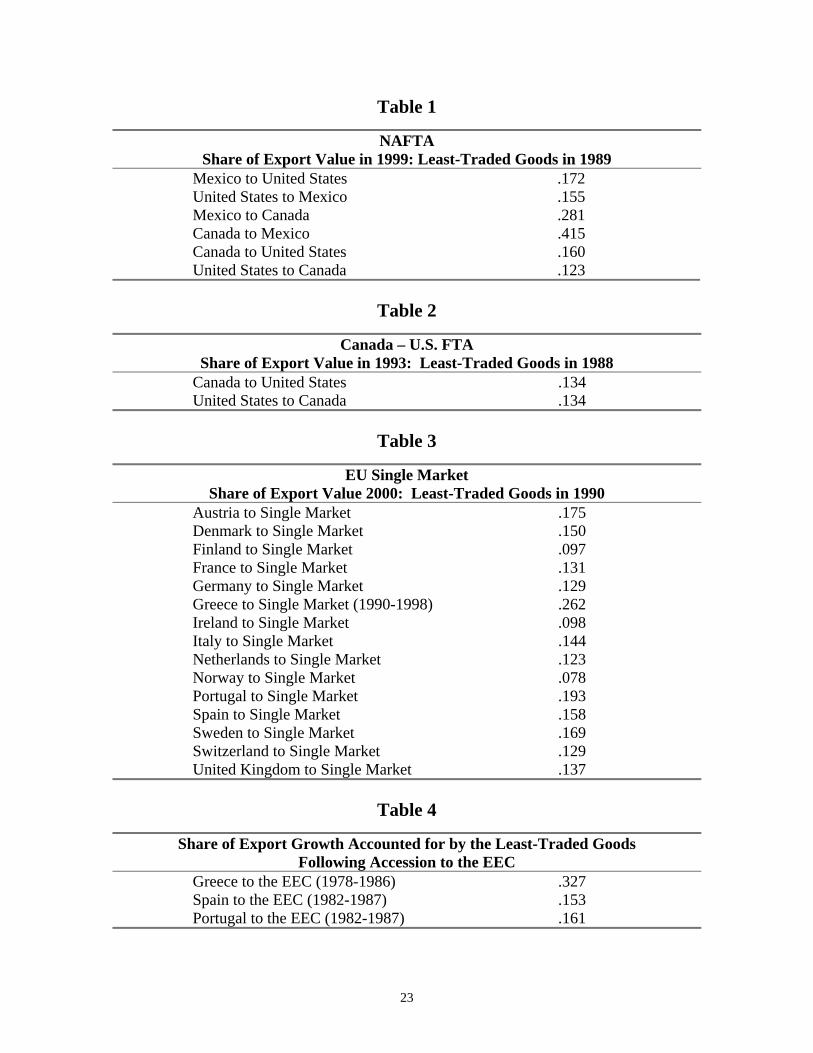
Table 1 lists the end of sample export shares of the least-traded goods for all of

the bilateral pairs associated with the NAFTA. The growth in the extensive margin is

present for all of the NAFTA trading pairs. For Canada and Mexico, the extensive

margin is particularly large, with Canadian least-traded goods growing to more than four

times its original trade share. A single code, unmilled wheat, accounts for almost half of

the growth in trade share, but the remaining half is distributed over the other 737 codes.

Rarely do single codes have an impact on our measure, as in the case of Canada and

8

Mexico. Growth in the extensive margin is smaller for the U.S. and Canada relationship,

but this is to be expected as the two countries had signed a bilateral free trade agreement

only five years prior to the NAFTA. Table 2 presents the results for the U.S.-Canada

FTA, in which it is clear that growth in the extensive margin had also occurred.

Figure 5 follows the trade share of the least-traded goods from Mexico to the U.S.

through the sample period. The sharp increase in the least-traded goods’ fraction of total

trade coincides exactly with the implementation of the NAFTA in 1994. Figure 6

presents the same measure for exports from Mexico to Canada. Following the NAFTA

liberalization, the least-traded goods’ trade share almost triples. In both cases the shares

had remained relatively constant prior to the NAFTA.

Further evidence of the growth in trade along the extensive margin is presented in

table 3, which provides detail for the countries involved in the European Union Single

Market.4 The Single Market entered into force on January 1, 1993 for the 12 EU

countries and was extended in 1994 to include the European Free Trade Association,

(EFTA) bringing the total number of countries involved to 19. Rather than report the 342

bilateral combinations, we aggregate exports to the other Single Market countries and

calculate the statistics as if they were one partner country. An inspection of table 3

reveals the substantial growth in the extensive margin for almost all of the countries

involved. For Italy, the least-traded goods’ increase their market share by more than 40

percent, with shares increasing by roughly 30 percent in countries such as France and the

United Kingdom. Trade growth in countries with little extensive margin growth are

almost always driven by a single commodity. In Norway, one subgroup – petroleum –

accounts for 73% of nominal trade growth, and communications equipment accounts for

more than half of Finland's nominal trade growth over the sample period.

The Single Market experience also highlights the timing of this growth. Figure 7

plots the trade share of the least-traded goods over the sample period for France and Italy,

who were two of the largest exporters of the Single Market countries. There are large

increases in the trade share of these least-traded goods between the years 1992 and 1993

4 As part of the EFTA, Iceland and Liechtenstein are also members of the Single Market, but are notincluded in this analysis, due to lack of data. Belgium and Luxembourg have also been excluded for lack ofconsistent data.

9

– coinciding exactly with the implementation of the Single Market. For France, the

export share increases approximately 30 percent in the first year of the Single Market.

Finally, we turn to the accessions of Greece, Portugal, and Spain to the European

Economic Community. Again we aggregate the EEC countries to create one partner

country with which to compile statistics. Table 4 presents the results. All three countries

show strong growth along the extensive margin, with Greece’s least-traded goods gaining

more than 300 percent in trade share. Figure 9 also makes clear the timing of this

growth. The trade share of Greece’s least traded goods jumps from .10 to .17 in just the

first year following its accession to the EEC, and by 1986, this share has climbed to .327.

3.1 Other Measures

As an alternative way of measuring the extensive margin, we modify the

decomposition used in Hummels and Klenow (2002) to apply to a single bilateral trade

relationship. The technique decomposes country 'i s share of world exports to country j

as

ij

iji

j Wjk

k K

xIntensive Export Margin

x∈

=∑

ij

Wjk

k Kij W

j

xExtensive Export Margin

x∈=∑

where the value of exports from country i to country j is denoted ijx , and W

jkx is the

value of exports from the world to country j of good k . The set ijK consists of all

SITC codes in which country i exports to country j . Thus, if country i exports many

different goods to j , it would have a higher extensive margin, whereas, if it exported

only a few goods to country j , it would have a higher intensive margin. Note that

multiplying the intensive margin by the extensive margin returns country 'i s share of

world exports to j , ij

Wj

xx

.

We further extend their measure to consider how the intensive and extensive

margins grow over the sample period. To do so, we compute the two statistics above for

10

each year in the sample period, generating a time series measurement of the intensive and

extensive margins. The results for the NAFTA pairs are shown in table 5. The first

column of table 5 shows the percentage growth rates of our measure of the external

margin. The second column shows the Hummels-Klenow (HK) decomposition in which

a good is considered not traded if and only if exports are equal to zero, as in Hummels

and Klenow (2002). The third column contains the HK decomposition computed with a

cutoff value of $50,000 as in Evenett and Venables (2002). Though our measure grows

much more than the HK decompositions, the ordering of countries is similar. The two

measures that employ fixed-value cutoffs find almost no growth in the U.S.-Canada

extensive margin, while the measures based on our relative cutoffs show modest growth.

The HK measures tell us why: the United States and Canada were already trading large

amounts (greater than $50,000) of almost every good.

If the U.S. and Canada are already trading large amounts of many goods, it is

difficult to pick up any extensive margin growth using fixed dollar definitions of

tradedness. The value of a good exported to the U.S. from Canada in the amount of

$71,376,000 accounts for only 0.08% of total trade from Canada to the U.S., and is

considered very traded by the fixed dollar measures considered. However, our relative

measure implies that all goods being exported at less than $71,376,000 between Canada

and the U.S. are “not traded.”5 To define these goods as traded in a fixed dollar measure

one needs to increase the cutoff, but this creates problems in other dimensions. In the

Canada to Mexico export data, a $71,376,000 cutoff would mean that a good valued at

14% of trade would be considered not traded.

The above example highlights the underlying tension in dollar-value definitions of

tradedness: a dollar value cutoff may understate the extensive margin in large trade

relationships, and overstate the extensive margin in small trade relationships. This can be

seen by comparing the Canada-U.S. trade relationship, which is big, to the Canada-

Mexico relationship, which is small.6 Computing the HK decomposition with a cutoff of

$50,000 implies that the Canada-Mexico extensive margin grows about 36 times faster

5 The $71,376,000 cutoff is the value of the highest-valued good in the set of least-traded goods forCanadian exports to the U.S in 1989.6 In 1989, Canadian exports to the U.S. totaled $80 billion, while Canadian exports to Mexico were $504million.

11

than the Canada-U.S. extensive margin. In comparison, our relative measure finds the

Canada-Mexico extensive margin growing at only 4 times the rate of the Canada-U.S.

extensive margin.

As a robustness check, we consider the choice of our cutoff level. In addition to

the 10% cutoff used in this paper, table 6 reports the extensive margin growth rates for

5% cutoffs and 20% cutoffs. Each column in table 6 reports the percentage growth rate

of the least traded goods for the given cutoff value. When we compute our measures

using 5% rather than 10% cutoffs, the least-traded goods grow faster in every country

except Denmark. Under the 5% cutoffs, Finland even switches sign, from a 3% decrease,

to an 11% increase. Ireland undergoes a similar change at the smaller cutoff. The

increased growth with smaller cutoffs supports the idea that goods with very small trade

shares are driving the extensive margin growth, and that our measure, if anything,

understates the amount of growth. The measure computed with 20% cutoffs grows

slower in all cases, and has a simple mean of roughly half the measure using 10% cutoffs.

As expected, larger cutoffs make the sets of goods too big to capture the growth in the

least-traded goods. The cutoffs also have little effect on the movement of the measures.

The correlation coefficients for the three series range from 0.98 to 0.99

The preceding exercise makes it clear that the extensive margin is an important

force in the growth in trade. The goods that make up only ten percent of trade prior to

liberalization regularly increase their share of trade by 30 percent or more following the

decrease in trade barriers. For some countries these goods’ share increases more than

four-fold. This important feature is not captured in most of the commonly used trade

models, such as the factor proportions or monopolisitc competition models. In the next

section we present a Ricardian model that is capable of reproducing this growth in the

extensive margin.

4. The ModelWe take as our point of departure the Ricardian model with a continuum of goods

as in Dornbusch, Fischer, and Samuelson (1977). We generalize the specification of

comparative advantage in order to provide a model that can be calibrated to match the

data on intra-industry trade.

12

There are two countries, ,i h f= and a continuum of goods indexed by [ ]0,1x ∈ .

Each country possesses the technology to produce every good, x , but with differing unit

costs.

( ) ( )( ) [ ]0,1

ii

i

l xy x x

a x= ∈

Each country is endowed with labor, iL which is the only factor of production.

There is a stand-in consumer is each country who chooses consumption and labor supply

in order to maximize

( )( )1

0

log iU c x dx= ∫

subject to the budget constraint

( ) ( )1

0

i i i ip x c x dx w L≤∫ ,

and thus expenditure on any good, x , is

( ) ( )i i i ic x p x w L= . (1)

Each country can levy an ad valorem tariff of iτ on imports, and tariff revenues are

wasted. We take home country labor as the numeraire, normalizing the home wage to

one. A good is imported if it is less costly to do so than to produce it at home. Thus, if

( ) ( ) ( )* * *1 a x w a xτ+ <

( )( ) ( )

*

* *1a x wa x τ

<+

good x is only produced in the home country and is exported to the foreign country. (As

is common, we use an asterisk to denote foreign country variables.) Similarly, if it is less

costly to produce good x in the foreign country,

( )( ) ( ) *

* 1a x

wa x

τ> +

the good will only be produced there, and will be exported to the home country.

For producing growth in the external margin, the arrangement

13

( ) ( )( ) ( )

**

* *1

1a x wwa x

ττ

+ < <+

(2)

is important. In this case, good x is produced in each country and is not traded. Goods

that fall into this range are nontraded for the given level of tariffs, but may become traded

as tariffs fall. Thus, the relative productivities of the two countries, along with the tariff

rates, and wages completely determine the pattern of trade in this model. Next, we turn

our attention to modeling relative productivity.

In the traditional expositions using this model, the relative productivities of the

two countries are ordered such that

( )( )

( )( )* * ,

a x a xx x such that x x

a x a x′

′ ′< ∀ <′

Although this formulation allows for an easy characterization of the trade pattern, it is

hard to imagine a way to apply this ordering to the trade data available. Two major

difficulties exist. First, trade data is collected in aggregates (such as SITC subgroups)

which do not easily correspond to a particular good. Even in the absence of the first

problem, one is still faced with measuring the unit costs (or relative productivities) of a

detailed good across many countries.

Instead of imposing another arbitrary ordering on the goods, we take advantage of

the ordering provided by the statisticians at the United Nations. The SITC defines

groupings based on degree of processing and use, rather than some other criteria, such as

major component of composition. For example, the Harmonized System groups wood

figurines and wood charcoal together as wood products, while the SITC classifies wood

charcoal into primaries, and figurines into wood manufactures. (Pasteels 1988) We apply

the SITC ordering rule to our product space. Thus, good 0000 lies on the left end of the

interval, and good 9999 lies on the right end of the interval. Given this ordering, SITC

codes are just intervals in [ ]0,1 . Having ordered the goods, we now proceed by assigning

relative productivities to each good.

Take J equally spaced points on [ ]0,1 . For each of these points, let jα denote

the log of the relative productivities of good jx .

14

( )( )*

log 1,...,jj

j

a xj J

a xα

= =

We assume that the log-relative productivities of these J goods are uniformly

distributed. The distribution is parameterized by a single parameter, α ,

[ ],j uα α α−!

which implies that the two countries, on average, have identical technologies. We

choose to work with the log-relative productivity schedule to keep the countries

symmetric. So that we can continue to work with a continuous product space, we

connect jα and 1jα + with a line, producing a continuous relative productivity schedule.

The key parameters in this model are α and J . For a given ,J α controls the

number of nontraded goods in the model by controlling the slope of the relative

productivity schedule's segments. The effect of α on the extensive margin can be seen in

figures 10 and 11. Here we present a stylized version of the relative productivity curve,

in which J is equal to 10, and only a few SITC codes are considered. For a good to be

nontraded, its relative productivity must lie between ( )* *1w τ+ and ( ) *1 wτ+ . As tariffs

fall, the gap between these two shrinks, and goods which were in this range, and now are

not, become traded. α is low in figure 10, and segments of the relative productivity

curve are not very steep. In this case, lowering tariffs induces trade in many goods not

previously traded. In figure 11 α is high, and these segments are steeper, so fewer goods

are forced out of the nontraded range defined by ( )* *1w τ+ and ( ) *1 wτ+ .

The number of points sampled in the interval, ,J also has an effect on the number

of nontraded goods in the model. More points imply smaller intervals between the

points, so for given values of 1andj jα α + , a higher value of J yields a steeper segment

of the relative productivity curve.

J and α also control the amount of intra-industry trade in the model. In order to

produce intra-industry trade, the relative productivity curve must lie both above ( ) *1 wτ+

and below ( )* *1w τ+ within one SITC code. Given J and the size of the SITC code,

higher values of α make the segments of the relative productivity curve steeper,

15

increasing the likelihood of it laying above and below the nontraded zone within one

code. The parameter J influences the amount of intra-industry trade by controlling the

number of times the relative productivity curve can change directions. If 2J = , for

example, the relative productivity curve would be a straight line between 1α and 2α , and

only one SITC code, at most, could have intra-industry trade. As J is increased, the

relative productivity curve, on average, changes direction more times, creating more

opportunities for the curve to pass through the nontraded zone within one SITC code. In

figures 10 and 11, the intervals marked on the horizontal axis represent individual SITC

codes. Notice that some codes are much smaller than others are – as in the data. In

figure 11, in which α is high, the shaded areas on the horizontal axis are the goods

traded intra-industry. There is no intra-industry trade in figure 10.

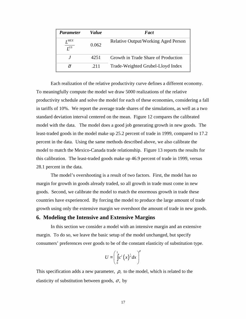
5. CalibrationTo calibrate this model we need to specify values for the size of each SITC code,

iL , J , and α . Below we consider calibrating the model to the Mexico-U.S. trade

relationship over the years 1989-1999.

The country size parameters are calibrated to the relative outputs of the countries

being considered. Using U.S. dollar GDP in 1989, the U.S. is about 20 times larger than

Mexico. Since we explicitly ordered the goods in our model according to their SITC

ordering, an SITC code is an interval in [ ]0,1 . To measure the size of each SITC code,

the ideal measure is the code’s share of total world output.

( )MEX USk k

k MEX USk k

k

y ysizey y

+=+∑

However, gross output data at the detailed, comparable, level is not available. We instead

measure SITC code size by its export share in trade. This is certainly an imperfect

measure, so we check the sensitivity of our results to this method in the next section. For

each SITC code, ,k we compute its share of total year 1989 trade.

( ), .MEX US

US k kMEX k MEX US

k kk

EX EXsizeEX EX

+=+∑

16

We assign an interval of length ,USMEX ksize to code k , in ascending order, such that

0011k = has 0 as its left endpoint, and 9999k = has 1 as its right endpoint.

It remains to specify values for J and α . These parameters jointly determine the

amount of intra-industry trade between the two countries and the increase in the value of

total trade following a decrease in tariffs. To measure intra-industry trade, we compute

the Grubel-Lloyd (1975) index at the four-digit SITC level for 1989, which is defined

below.

, ,,

, ,

1 100US MEXMEX k US kUS

MEX k US MEXMEX k US k

EX EXgl

EX EX

− = − × +

The index runs from 0, if there is no intra-industry trade, to 100, if the countries export as

much of the good as they import. We then weight each code’s Grubel-Lloyd value by its

share in total trade, creating a trade-weighted Grubel-Lloyd index.

, ,US US USMEX MEX k MEX k

k SITCWGL gl size

∈

= ∗∑

The trade weighted Grubel-Lloyd index in 1989 is 48.7, reflecting substantial intra-

industry trade between the United States and Mexico.

To measure the growth in trade, we calculate the fraction of U.S. and Mexican

production that is traded in 1989 and 1999. Since trade data is measured as shipment

value, and not GDP, gross output is the correct measure of production. We include only

the production of primaries and manufactures, as our trade data covers only these two

commodity types. We also adjust output to match the structure of our two-country

model. To do this, we exclude production that is traded to other countries, by subtracting

exports to these countries from gross output. This yields a measure of output that is

either consumed domestically, or traded to the partner country—the only two possibilities

in the model. We use the geometric average of the two countries’ shares. This average

share increased 202% over the sample period.

17

Parameter Value FactMEX

US

LL

0.062Relative Output/Working Aged Person

J 4251

α .211

Growth in Trade Share of Production

Trade-Weighted Grubel-Lloyd Index

Each realization of the relative productivity curve defines a different economy.

To meaningfully compute the model we draw 5000 realizations of the relative

productivity schedule and solve the model for each of these economies, considering a fall

in tariffs of 10%. We report the average trade shares of the simulations, as well as a two

standard deviation interval centered on the mean. Figure 12 compares the calibrated

model with the data. The model does a good job generating growth in new goods. The

least-traded goods in the model make up 25.2 percent of trade in 1999, compared to 17.2

percent in the data. Using the same methods described above, we also calibrate the

model to match the Mexico-Canada trade relationship. Figure 13 reports the results for

this calibration. The least-traded goods make up 46.9 percent of trade in 1999, versus

28.1 percent in the data.

The model’s overshooting is a result of two factors. First, the model has no

margin for growth in goods already traded, so all growth in trade must come in new

goods. Second, we calibrate the model to match the enormous growth in trade these

countries have experienced. By forcing the model to produce the large amount of trade

growth using only the extensive margin we overshoot the amount of trade in new goods.

6. Modeling the Intensive and Extensive MarginsIn this section we consider a model with an intensive margin and an extensive

margin. To do so, we leave the basic setup of the model unchanged, but specify

consumers’ preferences over goods to be of the constant elasticity of substitution type.

( )1

1

0

iU c x dxρ

ρ

= ∫

This specification adds a new parameter, ,ρ to the model, which is related to the

elasticity of substitution between goods, ,σ by

18

11

σρ

=−

.

As is common with this specification of preferences, we can think of U as a composite

good, and derive the price of this good as

( )1

1 11

0

i iP p x dxσσ −−

= ∫

and the expenditure on any good as

( ) ( ) ( ) 1ii i i i

i

p xc x p x w L

P

σ−

=

. (3)

The above relation is the key difference between the model with and without the internal

margin. Suppose that good x is already traded. In the model with only the extensive

margin we can see from (1) that expenditure on this good remains unchanged following

the decrease in tariffs. However, as can be seen in (3), as tariffs are lowered and the

delivered price falls, expenditure on this good will increase following the decrease in

tariffs, given that 1σ > . This internal margin growth should relieve some of the

responsibility for generating trade growth that was before solely shouldered by the

extensive margin.

In the model with Cobb-Douglas preferences, we did not have to keep track of the

prices of the goods, since expenditure on each good was constant at i iw L . Under the

more general CES preferences, we need all of the prices to solve the model, and to know

the prices, we must know all the unit costs, rather than just the ratios. We use the same

uniform distribution to assign the ratio of log relative productivities, and pin down the

unit cost levels with a normalization. We assume that * 1,j ja a = so the log

productivities are fractions of the relative productivity.

( )( ) ( )( )log log * 1,...,2 2

j jj ja x a x j J

α α= = − =

We solve this version of the model as we did the earlier one, by drawing 5000

relative productivity schedules, solving the model and averaging across the realizations.

We calibrate this version of the model to the same facts as before. We treat the elasticity

of substitution parametrically, and seek parameters such that the model’s results match

19

the observed extensive margin growth in the data. Figures 14 and 15 compare the

model’s results with the data. In the case of Mexico and Canada, we needed an elasticity

of 12.35 in order to match the extensive growth of 28.1 percent found in the data. In the

case of Mexico and the United States, an elasticity of substitution around 14 is needed to

match the data.

The elasticities needed to match the model to the data are a bit higher than those

found in the literature. These high elasticities are also the result of forcing the model to

produce the growth in aggregate trade levels. A major problem in the international trade

literature is the inability of the workhorse models to produce the large observed growth in

trade given the small observed change in tariffs. Basic monopolistic competition models,

international real business cycle models, and even the Ricardian model, on which our

model is built, suffer from this problem.7 Given this inherited (and common) problem,

our model performs as well as the standard models in producing the aggregate trade

growth. Where it advances beyond these models is in its ability to reproduce the

observed extensive margin growth, and provide a simple Ricardian economy that can be

calibrated.

7. Sensitivity AnalysisThe use of trade flows as a proxy for output in measuring the size of an SITC

code is potentially a source of concern. Some industries may export a larger fraction of

their output than might others, leading to a very different “industry size” when measured

by trade share rather than production share. However, this problem may not be as

worrisome as it first seems. Since we are not making predictions about individual

industries, the idea that an industry may be measured as “large” by output and “small” by

trade volume is not necessarily a problem. If this industry is offset by another that is

measured “small” by output and “large” by trade volume, our results should be

unaffected. We only need the distribution of industry sizes to be similar. In this section

we check the sensitivity of the model’s results to our choice of measurement.

7 See Yi (2002) for an overview of the failure of these models in this area. He shows that elasticities ofsubstitution in the range of 12 to 14 are needed in these models to match the observed U.S. trade growthgiven a 15% tariff reduction.

20

Data on production (gross output -- not value added) is particularly difficult to

obtain at a very disaggregated level, particularly comparable data for many countries. In

order to keep the data comparable across countries; we collect data on gross output from

Mexico and the United States at the four-digit level of the International Standard

Industrial Classification (ISIC). Unfortunately, this yields only 96 different groups,

compared to the 789 four-digit SITC codes. We map the SITC codes into the ISIC

groups, and divide the production value from each ISIC group evenly across the relevant

SITC codes. This crude mapping yields a series of gross output by SITC codes, which is

then normalized to lie in the unit interval as described above in the calibration section.

Figure 16 compares the two series. The two methods produce series that are very

similar except for the largest industries. The ten largest industries as measured by trade

volume are, on average, 6.6 times larger than the ten largest industries by production.

Much of this difference is probably driven by the equal assignment of production values

to indistinguishable SITC codes under our crude concordance.

Given the difference in the large industries between the two methods, it is

worthwhile to see how the model’s results change using the production series. We

recalibrate the Mexico-U.S. model exactly as before, except we use the production

numbers to create the SITC codes on the unit interval. The most significant change in the

parameter values is the higher value of ,J the number of times the relative productivity

curve can change directions. In the model, large industries tend to have more intra-

industry trade, so shrinking the largest industries requires the intra-industry trade be made

up in the other industries. To get more intra-industry trade in the smaller industries, on

average, we need the relative productivity curve to change directions more often, creating

more chances for intra-industry trade.

The results of the model under the two different measuring schemes are shown in

Figure 17. The model using the output measure produces an export share of .186 for the

least-traded goods, compared to the .172 share in the model using the trade measure.

Using the trade data, our mapping created a series with a few large industries, whereas

the output data creates a series containing no large industries. Given that the true

distribution of industry size lies somewhere in-between the two, the small spread between

21

the results suggests our results are robust to measurement error in the size of the SITC

codes.

8. Concluding RemarksWe have provided evidence of an important, yet little discussed feature of trade

growth – the extensive margin. After studying six major trade liberalizations, we find

that trade in goods that were not before traded shows substantial growth following a

decrease in trade barriers. For some countries, the collection of goods that accounted for

only 10 percent of trade prior to the liberalization more than quadruples its share in only a

few years following the liberalization. This fact is particularly important given that most

applied international trade models do not include an extensive margin, and have trouble

accounting for the large increases in trade following a relatively small decrease in tariffs.

By modifying a standard Ricardian model, we provide a model that is capable of

reproducing this growth in the extensive margin.

22

References

BORDE, F. (1990): “A Database for Analysis of International Markets,” CanadianStatistical Review.

DORNBUSCH, R., S. FISCHER, AND P. SAMUELSON (1997): “ComparativeAdvantage, Trade and Payments in a Ricardian Model with a Continuum of Goods,”American Economic Review, pp. 823-829.

EVENETT, S.J., and A.J. VENABLES (2002): “Export Growth in Developing Countries:Market Entry and Bilateral Trade Flows.” mimeo

FEENSTRA, R. (1992): “How Costly is Protectionism?” The Journal of EconomicPerspectives, pp159-178.

FEENSTRA, R. (2000): “World Trade Flows, 1980-1997,” Center for InternationalData, UC Davis.

FEENSTRA, R., R. LIPSEY, AND H. BOWEN (1997): “World Trade Flows, 1970-1992with Production and Tariff Data,” NBER Working Paper 5910.

GRUBEL, H. G., AND P.J. LLOYD (1975) Intra Industry Trade, London: Macmillan.

KEHOE, T.J. (2002): “An Evaluation of the Performance of Applied GeneralEquilibrium Models of the Impact of NAFTA,” Federal Reserve Bank of Minneapolis.

KLENOW, P.J. AND A. RODRIGUEZ-CLARE(1997): “Quantifying Variety Gains fromTrade Liberalization,” University of Chicago.

KRAAY, A., AND J. VENTURA (2002): “Trade Integration and Risk Sharing,” NBERWorking Paper 8804.

MOZES, S., AND D.OBERG (2001): “U.S. – Canada Data Exchange, 1990-2001,”Statistics Canada and U.S. Census Bureau.

NICITA, A., AND M. OLARREAGA (2001): “Trade and Production, 1976-1999,” TheWorld Bank.

PASTEELS, J.-M. (1998): “Foreign Trade Statistics: A Basic Market Research Tool,”International Trade Centre UNCTAD/WTO.

ROMER, P. (1994): “New Goods, Old Theory, and the Welfare Costs of TradeRestrictions,” Journal of Development Economics, pp. 5-38.

YI, K.-M. (2001): “Can Vertical Specialization Explain the Growth in World Trade?,”forthcoming, Journal of Political Economy.

23

Table 1

NAFTAShare of Export Value in 1999: Least-Traded Goods in 1989

Mexico to United States .172United States to Mexico .155Mexico to Canada .281Canada to Mexico .415Canada to United States .160United States to Canada .123

Table 2

Canada – U.S. FTAShare of Export Value in 1993: Least-Traded Goods in 1988

Canada to United States .134United States to Canada .134

Table 3

EU Single MarketShare of Export Value 2000: Least-Traded Goods in 1990

Austria to Single Market .175Denmark to Single Market .150Finland to Single Market .097France to Single Market .131Germany to Single Market .129Greece to Single Market (1990-1998) .262Ireland to Single Market .098Italy to Single Market .144Netherlands to Single Market .123Norway to Single Market .078Portugal to Single Market .193Spain to Single Market .158Sweden to Single Market .169Switzerland to Single Market .129United Kingdom to Single Market .137

Table 4

Share of Export Growth Accounted for by the Least-Traded GoodsFollowing Accession to the EEC

Greece to the EEC (1978-1986) .327Spain to the EEC (1982-1987) .153Portugal to the EEC (1982-1987) .161

24

Table 5NAFTA Growth Rates (%)

Kehoe-Ruhl10% Cutoff

Hummels-Klenow$0 Cutoff

Hummels-Klenow$50,000 Cutoff

Hummels-KlenowImplied Cutoffs

U.S. to CAN 10.0 0.0 0.0 11.2CAN to U.S. 72.0 1.5 2.0 34.2U.S. to MEX †35.0 9.1 9.2 17.1MEX to US 78.0 1.4 2.0 28.3MEX to CAN 173.0 15.0 23.7 47.2CAN to MEX †417.0 25.0 73.4 171.0

†Data on Exports from the world to Mexico are only available for 1990 and onward. Thus, we report our measure spanning 1989-1999, which is why these numbers differ from the ones in table 1.

Table 6Results Under Different Cutoff Values

Percentage Growth Rate of Export Share: Least-Traded Goods5% 10% 20%

Mexico to U.S. (1989-1999) 128.7 71.7 32.8U.S. to Mexico (1989-1999) 54.3 55.0 38.8Mexico to Canada (1989-1999) 354.9 180.8 102.9Canada to Mexico (1989-1999) 610.5 315.1 171.8Canada to U.S. (1989-1999) 101.0 59.9 37.2U.S. to Canada (1989-1999) 47.7 23.2 13.5Canada to U.S. (1988-1993) 57.1 34.2 18.9U.S. to Canada (1988-1993) 47.2 34.3 21.3Austria to Single Market (1990-2000) 137.7 74.8 36.0Denmark to Single Market (1990-1999) 43.8 50.1 29.7Finland to Single Market (1990-2000) 10.9 -3.2 -17.3France to Single Market (1990-2000) 71.6 31.5 16.1Germany to Single Market (1990-1999) 64.8 29.2 10.6Greece to Single Market (1990-2000) 263.9 162.0 75.9Ireland to Single Market (1990-2000) 43.1 -2.5 4.6Italy to Single Market (1990-2000) 69.0 43.5 26.0Netherlands to Single Market (1990-2000) 32.1 23.0 14.1Norway to Single Market (1990-2000) -14.6 -22.4 -27.0Portugal to Single Market (1990-2000) 140.1 92.7 46.0Spain to Single Market (1990-2000) 74.1 58.0 30.7Sweden to Single Market (1990-2000) 142.0 68.7 28.2Switzerland to Single Market (1990-1999) 34.6 28.9 14.5U.K. to Single Market (1990-2000) 36.7 36.7 9.9Greece to EEC (1978-1986) 451.0 227.4 99.2Spain to EEC (1982-1987) 98.6 53.1 35.5Portugal to EEC (1982-1987) 123.3 61.5 38.1Average 124.0 68.7 34.9

Corr(5%, 10%) = .985 Corr(10%, 20%) = .981 Corr(5%,20%) = .959

Figure 1

Composition of ExportsSets of Categories Based on Export Size

0.0

0.1

0.2

0.3

0.4

0.1 0.2 0.3 0.4 0.5 0.6 0.7 0.8 0.9 1.0Cummulative Fraction of Exports: Beginning of Sample Period

Frac

tion

of E

xpor

ts: E

nd o

f Sam

ple

Perio

d

Figure 2

Composition of ExportsSets of Categories Based on Export Size

0.0

0.1

0.2

0.1 0.2 0.3 0.4 0.5 0.6 0.7 0.8 0.9 1.0Cummulative Fraction of Exports: Beginning of Sample Period

Frac

tion

of E

xpor

ts: E

nd o

f Sam

ple

Perio

d

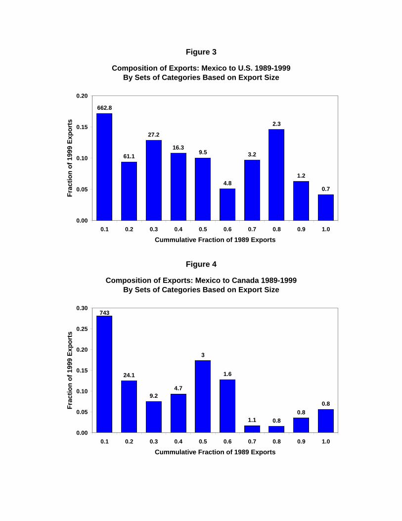
Figure 3

Composition of Exports: Mexico to U.S. 1989-1999By Sets of Categories Based on Export Size

0.7

1.2

2.3

3.2

4.8

9.516.3

27.2

61.1

662.8

0.00

0.05

0.10

0.15

0.20

0.1 0.2 0.3 0.4 0.5 0.6 0.7 0.8 0.9 1.0

Cummulative Fraction of 1989 Exports

Frac

tion

of 1

999

Expo

rts

Figure 4

Composition of Exports: Mexico to Canada 1989-1999By Sets of Categories Based on Export Size

0.80.8

0.81.1

1.6

3

4.79.2

24.1

743

0.00

0.05

0.10

0.15

0.20

0.25

0.30

0.1 0.2 0.3 0.4 0.5 0.6 0.7 0.8 0.9 1.0

Cummulative Fraction of 1989 Exports

Frac

tion

of 1

999

Expo

rts

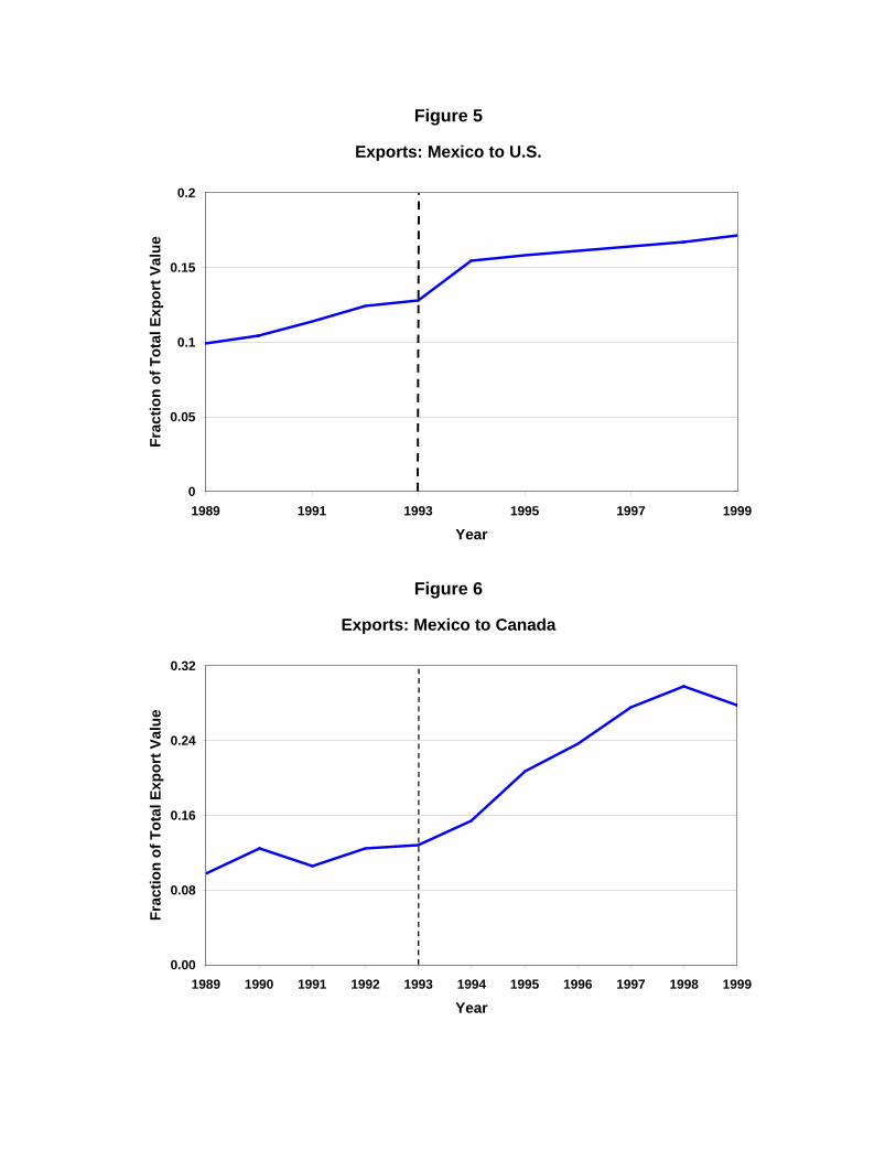
Figure 5

Exports: Mexico to U.S.

0

0.05

0.1

0.15

0.2

1989 1991 1993 1995 1997 1999

Year

Frac

tion

of T

otal

Exp

ort V

alue

Figure 6

Exports: Mexico to Canada

0.00

0.08

0.16

0.24

0.32

1989 1990 1991 1992 1993 1994 1995 1996 1997 1998 1999

Year

Frac

tion

of T

otal

Exp

ort V

alue

Figure 7

Exports to the Single Market

0.00

0.05

0.10

0.15

1990 1991 1992 1993 1994 1995 1996 1997 1998 1999 2000

Year

Frac

tion

of T

otal

Exp

ort V

alue

France

Italy

Figure 8

Composition of Exports: Greece to the EEC 1979-1986By Sets of Categories Based on Export Size

1.11.82.7

33.5

4.1

5.8

10.6

23.9

732.6

0.00

0.05

0.10

0.15

0.20

0.25

0.30

0.35

0.1 0.2 0.3 0.4 0.5 0.6 0.7 0.8 0.9 1.0

Cummulative Fraction of 1979 Exports

Frac

tion

of 1

986

Expo

rts

Figure 9

Exports: Greece to EEC

0.00

0.05

0.10

0.15

0.20

0.25

0.30

0.35

1979 1980 1981 1982 1983 1984 1985 1986

Year

Frac

tion

of T

otal

Exp

ort V

alue

Figure 10

Figure 11

x

( )( )*

a xa x

( )*w*1+τ w

( ) *1+τ w

( )( )*

a xa x

x

( )*w*1+τ

( ) *1+τ w

Figure 12

Composition of Exports: Mexico to U.S. 1989-1999By Sets of Categories Based on Export Size

0.00

0.05

0.10

0.15

0.20

0.25

0.30

0.1 0.2 0.3 0.4 0.5 0.6 0.7 0.8 0.9 1.0

Cummulative Fraction of 1989 Exports

Frac

tion

of 1

999

Expo

rts

Data

Model

Two Standard Deviations

Figure 13

Composition of Exports: Mexico to Canada 1989-1999By Sets of Categories Based on Export Size

0.0

0.1

0.2

0.3

0.4

0.5

0.6

0.1 0.2 0.3 0.4 0.5 0.6 0.7 0.8 0.9 1.0

Cummulative Fraction of 1989 Exports

Frac

tion

of 1

999

Expo

rts

DataModel

Two Standard Deviations

Figure 14

Composition of Exports: Mexico to U.S. 1989-1999By Sets of Categories Based on Export Size

0.00

0.05

0.10

0.15

0.20

0.25

0.1 0.2 0.3 0.4 0.5 0.6 0.7 0.8 0.9 1.0

Cummulative Fraction of 1989 Exports

Frac

tion

of 1

999

Expo

rts

DataModel

Two Standard Deviations

Figure 15

Composition of Exports: Mexico to Canada 1989-1999By Sets of Categories Based on Export Size

0.00

0.10

0.20

0.30

0.40

0.1 0.2 0.3 0.4 0.5 0.6 0.7 0.8 0.9 1.0

Cummulative Fraction of 1989 Exports

Frac

tion

of 1

999

Expo

rts

Two Standard Deviations

DataModel

Figure 16

Industry Size Measured by Trade Volume and Gross Output

0

100

200

300

400

500

600

0 0.1 0.2 0.3 0.4 0.5 0.6 0.7 0.8 0.9 1 1+Industry Share in Total Trade Volume or Gross Output (%)

Num

ber o

f Ind

ustr

ies

Measured by Trade

Measured by Gross Output

Figure 17

Composition of Exports: Mexico to U.S. 1989-1999 By Sets of Categories Based on Export Size

0.00

0.05

0.10

0.15

0.20

0.1 0.2 0.3 0.4 0.5 0.6 0.7 0.8 0.9 1.0 Fraction of 1989 Exports

Frac

tion

of 1

999

Expo

rts

Industries Measured by Exports

Industries Measured by Output

Appendix A

The Family TreeIn general, the data on trade flows is collected by the customs agents of the

individual countries. Depending on the year and country, this data may be collected under

various different systems of commodity classification. For example, the United States

collected data on imports and exports under the Tariff Schedule of the United States

Annotated (TSUSA) system and the “Schedule B,” respectively, until it adopted the

Harmonized System (HS) in 1989. Canada also used a national classification system,

while most European countries used the Customs Cooperation Council Nomenclature

(CCCN) or a derivation of it.

The customs data is then compiled by international institutions to produce usable

datasets. For example, the United Nations receives data from the reporting countries,

translates it into a common classification system, and makes it available as its

COMTRADE database. COMTRADE covers bilateral flows by commodity for a large

number of countries, and is the starting point for other derived datasets such as the World

Bank's Trade and Production, or Statistics Canada's World Trade Analyzer. (Nicita and

Olarreaga 2001, Feenstra 2000) The UN's system of classification is the broadly accepted

Standard International Trade Classification (SITC), which is currently in its third

revision. It consists of 10 sections (1-digit), 67 divisions (2-digit), 261 groups (3-digit),

1033 subgroups (4-digit), and 3121 items (5-digit).

International Trade by Commodity StatisticsThe ITCS database (formerly Foreign Trade by Commodity) is a collection of

three smaller databases, each differentiated by product classification and years covered.

The SITC.R2 database covers the years 1961-2000, while the HS and SITC.R3 databases

are available for only the years 1990 onward. The reporting countries in these databases

consist of the OECD member countries plus China, Hong Kong, and Chinese Taipei.

Each member country reports its trade with 264 other partner countries. Data is available

for value and quantity of goods traded -- though not all data is available for all country

pairs and years.

Prior to 1988, the OECD received the data from member countries classified

according to the SITC.R2. Subsequent to 1988, the OECD receives the data in HS format,

and converts it into the SITC.R2 and SITC.R3 classifications. The OECD makes few

modifications to the original data.

World Trade Flows (Feenstra 2000)In contrast, the World Trade Flows (WTF) dataset has been constructed with

special regard for consistency and comparability. The WTF dataset begins life as data

from the UN, which is then processed by Statistics Canada to produce the World Trade

Analyzer(WTA). The WTA is presented in Feenstra (2000) in both its original form, and

converted to the Bureau of Economic Analysis' industry classification. The WTF dataset,

documented in Feenstra (2000), which covers the period 1980-1997 for approximately

230 countries, is an update to the WTF dataset in Feenstra, Lipsey, and Bowen (1997)

which covers the years 1970-1992 and also features tariff and production data. The

dataset does not contain all country pairs for all years.

Rather than report a flow from country A to country B as both country A's exports

and country B's imports, Statistics Canada reports only one flow, which has been adjusted

in an attempt to provide a consistent and accurate report. Statistics Canada benchmarks a

country's total exports to the International Monetary Fund's Direction of Trade Statistics

figure for total world imports from that country. Statistics Canada then attempts to

allocate data unclassified by country using partner country records and adjusts for freight

and insurance costs. For further details see Borde (1990) and Feenstra (2000).

Though the WTA dataset is based on the SITC four-digit classification, the codes

reported in the documentation do not map into standard SITC codes exactly. (Feenstra

2000) Statistics Canada combined categories in order to provide a dataset more

comparable with Canadian data, and to deal with inconsistencies in the data. For

example, the WTA features categories ending in “X”, which represent unclassified trade

in a particular commodity. Subgroup 683X contains the value of unclassified shipments

of Nickel. Without the “X” subgroup, summing all the 68** subgroups would not yield

the same value as the listing for division 68. This procedure sacrifices a significant

amount of detail. For example, U.S.-Canada export data contains only 466 categories in

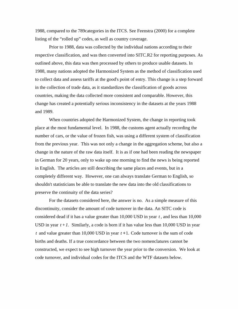
1988, compared to the 789categories in the ITCS. See Feenstra (2000) for a complete

listing of the “rolled up” codes, as well as country coverage.

Prior to 1988, data was collected by the individual nations according to their

respective classification, and was then converted into SITC.R2 for reporting purposes. As

outlined above, this data was then processed by others to produce usable datasets. In

1988, many nations adopted the Harmonized System as the method of classification used

to collect data and assess tariffs at the good's point of entry. This change is a step forward

in the collection of trade data, as it standardizes the classification of goods across

countries, making the data collected more consistent and comparable. However, this

change has created a potentially serious inconsistency in the datasets at the years 1988

and 1989.

When countries adopted the Harmonized System, the change in reporting took

place at the most fundamental level. In 1988, the customs agent actually recording the

number of cars, or the value of frozen fish, was using a different system of classification

from the previous year. This was not only a change in the aggregation scheme, but also a

change in the nature of the raw data itself. It is as if one had been reading the newspaper

in German for 20 years, only to wake up one morning to find the news is being reported

in English. The articles are still describing the same places and events, but in a

completely different way. However, one can always translate German to English, so

shouldn't statisticians be able to translate the new data into the old classifications to

preserve the continuity of the data series?

For the datasets considered here, the answer is no. As a simple measure of this

discontinuity, consider the amount of code turnover in the data. An SITC code is

considered dead if it has a value greater than 10,000 USD in year t , and less than 10,000

USD in year t +1. Similarly, a code is born if it has value less than 10,000 USD in year

t and value greater than 10,000 USD in year 1.t + Code turnover is the sum of code

births and deaths. If a true concordance between the two nomenclatures cannot be

constructed, we expect to see high turnover the year prior to the conversion. We look at

code turnover, and individual codes for the ITCS and the WTF datasets below.

Consistency of the ITCSThe International Trade by Commodity Statistics dataset allows for the study of

the same trade-flow measured by two different countries under different nomenclatures.

Here we consider the flow of goods from Canada to the United States, measured by both

Canada (as exports) and the U.S. (as imports). Turnover in the ITCS dataset displays the

pattern consistent with a poor concordance. (See Table A1) For data collected in Canada,

the code turnover is highest in 1987, reflecting the reorganization of the coding system in

1988. For the U.S.-collected data, turnover is highest in 1988, the year prior to the

adoption of the Harmonized System. In the Canadian-collected data, 343 of 789 codes

were turned over in 1987. The high turnover is driven by the 332 new codes put into

service in 1988, as more detailed source data became available.

The problems with this concordance, and the data in general, can be further seen

by inspecting individual codes. Figure A1 shows the value of Canadian Iron Castings

(SITC 6794) exported to the United States. Immediately obvious is the large discrepancy

in the pre 1990 data. Prior to 1989, the U.S. did not even record an entry for this product,

while Canada records its exports as tens of millions of dollars. This problem is well

known, and led to the U.S.-Canada Data Exchange, under which each country compiles

its export statistics using the other country's import data. This program is responsible for

the parity of the two series after 1990. (Mozes and Oberg 2001) There is a more subtle

inconsistency, however, with which we must concern ourselves. Notice the timing of the

large jumps in the two series. The Canadian-measured series display a large change

between 1987 and 1988, while the U.S.-measured series jumps between 1988 and 1989.

The timing of this reallocation of trade values coincides exactly with the two countries'

adoption of the Harmonized System. This problem is not unique to situations in which

one country was using a particular code while the other country was not. Figure 2

provides detail on exports of Transmission parts, a category used by both countries

throughout the sample, and a category consistently measured by both countries. The data

displays the same patterns. In fact, the problems outlined above are present throughout

the dataset.

Consistency of WTFThe statistics on turnover in this data display the same patterns seen in the ITCS.

(See Table A2) Turnover is highest in the year preceding adoption of the Harmonized

System, implying that these problems are present in this dataset, as well. It is also

interesting to note the high turnover in 1989, which appears to be reflecting the further

revisions of the two countries' statistics under the U.S.-Canada Data Exchange.

The WTF dataset only reports a flow as measured by the exporting country, so we

consider the Canadian-collected flow of goods from Canada to the United States, and the

U.S.-collected flow of goods from the United States to Canada for the years 1980-1997.1

Figures 3 and 4 present the two codes considered for the ITCS, but with data taken from

the WTF dataset. These figures must be viewed carefully. Given the single-valued

nature of the dataset, we cannot consider the same flow measured by each country. What

is presented instead, is each country's exports of the product, as measured by that country.

These figures are silent on the country-specific mismeasurement, but do provide evidence

on the problems associated with the adoption of the Harmonized System. For each of the

codes considered, the U.S.-collected series displays a break between 1888 and 1989,

while the Canadian-collected series break at 1987.

These simple exercises highlight the problems associated with the reclassification

of goods following the adoption of the Harmonized System. Detailed data is not

consistent before and after a country's adoption of the Harmonized System. These

changes affected the single source of the raw data, creating a problem that is likely

present in all of the datasets available. It should be noted that these problems are the

most serious in countries that made the change from a national classification scheme to

the HS, such as the United States, Canada, and Russia. Countries that were previously

using the CCCN, upon which the HS is based, seem to be much less affected by this

change.

1 Note that we are only measuring changes in the categories used by each country, so the fact that Canadamay export a different set of goods than the U.S. is not cause for concern.

Table A1

International Trade by Commodity StatisticsYear Canadian - Collected Data U.S. - Collected Data

Turnover Births Deaths Turnover Births Deaths1980 6 2 4 31 6 251981 5 4 1 32 20 121982 4 4 0 31 18 131983 0 0 0 30 8 221984 2 0 2 38 20 181985 3 0 3 24 10 141986 3 2 1 26 15 111987 343 332 11 24 8 161988 27 7 20 81 24 571989 39 15 24 34 16 181990 23 10 13 22 13 91991 25 11 14 27 14 131992 25 13 12 27 14 131993 29 14 15 28 14 141994 27 18 9 29 11 181995 17 8 9 14 7 71996 29 24 5 20 11 9

Table A2

World Trade Flows (Feenstra 2000)Year Canadian - Collected Data U.S. – Collected Data

Turnover Births Deaths Turnover Births Deaths1980 6 2 4 5 3 21981 3 2 1 2 0 21982 6 5 1 4 0 41983 1 1 0 5 3 21984 2 0 2 7 2 51985 1 0 1 5 4 11986 2 2 0 4 1 31987 23 17 6 4 2 21988 7 0 7 18 11 71989 15 9 6 14 8 61990 4 2 2 1 0 11991 7 3 4 5 3 21992 4 1 3 7 0 71993 7 4 3 3 2 11994 7 6 1 2 0 21995 4 3 1 3 2 11996 4 2 2 2 1 1

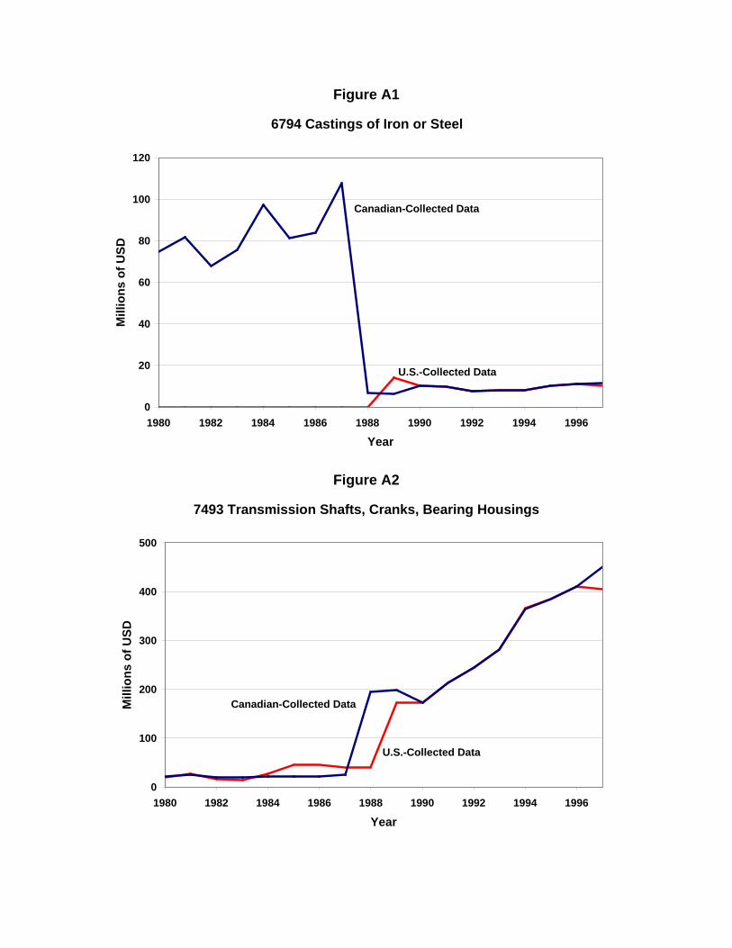
Figure A1

6794 Castings of Iron or Steel

0

20

40

60

80

100

120

1980 1982 1984 1986 1988 1990 1992 1994 1996

Year

Mill

ions

of U

SD

Canadian-Collected Data

U.S.-Collected Data

Figure A2

7493 Transmission Shafts, Cranks, Bearing Housings

0

100

200

300

400

500

1980 1982 1984 1986 1988 1990 1992 1994 1996

Year

Mill

ions

of U

SD

U.S.-Collected Data

Canadian-Collected Data

Figure A3

6794 Castings of Iron or Steel

0

40

80

120

1980 1982 1984 1986 1988 1990 1992 1994 1996

Year

Mill

ions

of U

SD

Canadian Exports(measured by Canada)

U.S. Exports(measured by U.S.)

Figure A4

7493 Transmission Shafts, Cranks, Bearing Housings

0

150

300

450

600

750

1980 1982 1984 1986 1988 1990 1992 1994 1996

Year

Mill

ions

of U

SD

Canadian Exports(measured by Canada)

U.S. Exports(measured by U.S.)

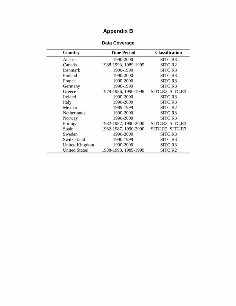
Appendix B

Data Coverage

Country Time Period ClassificationAustria 1990-2000 SITC.R3Canada 1988-1993, 1989-1999 SITC.R2Denmark 1990-1999 SITC.R3Finland 1990-2000 SITC.R3France 1990-2000 SITC.R3Germany 1990-1999 SITC.R3Greece 1979-1986, 1990-1998 SITC.R2, SITC.R3Ireland 1990-2000 SITC.R3Italy 1990-2000 SITC.R3Mexico 1989-1999 SITC.R2Netherlands 1990-2000 SITC.R3Norway 1990-2000 SITC.R3Portugal 1982-1987, 1990-2000 SITC.R2, SITC.R3Spain 1982-1987, 1990-2000 SITC.R2, SITC.R3Sweden 1990-2000 SITC.R3Switzerland 1990-1999 SITC.R3United Kingdom 1990-2000 SITC.R3United States 1988-1993, 1989-1999 SITC.R2