HOW IMPORTANT ARE TERMS‐OF‐TRADE SHOCKS?mu2166/tot/paper.pdf · HOW IMPORTANT ARE TERMS-OF ......

INTERNATIONAL ECONOMIC REVIEWVol. 59, No. 1, February 2018

HOW IMPORTANT ARE TERMS-OF-TRADE SHOCKS?∗

BY STEPHANIE SCHMITT-GROHE AND MARTIN URIBE 1

Columbia University, CEPR, and NBER, U.S.A.; Columbia University and NBER, U.S.A.

According to conventional wisdom, terms-of-trade shocks represent a major source of business cycles inemerging and poor countries. This view is largely based on the analysis of calibrated business-cycle models. Weargue that the view that emerges from empirical structural vector autoregression (SVAR) models is strikinglydifferent. We estimate country-specific SVARs using data from 38 countries and find that terms-of-trade shocksexplain less than 10% of movements in aggregate activity. We then estimate key structural parameters of athree-sector business-cycle model country by country and find a disconnect between the importance assigned toterms-of-trade shocks by theoretical and SVAR models.

1. INTRODUCTION

The conventional wisdom is that terms-of-trade shocks represent a major source of businesscycles in emerging and poor countries. This view is largely based on the analysis of calibratedbusiness-cycle models. Essentially, this result is obtained by first estimating a process for theterms of trade and then feeding it to an equilibrium business-cycle model to compute the vari-ance of macroeconomic indicators of interest induced by this type of disturbance. Then thisvariance is compared to the observed unconditional variance of the corresponding macroeco-nomic indicator to obtain the share of variance explained by terms-of-trade shocks. Consistently,this methodology arrives at the conclusion that more than 30% of the variance of output andother macroeconomic indicators is attributable to terms-of-trade shocks (Mendoza, 1995; Kose,2002).

In this article, we argue that there is a disconnect between theoretical and empirical modelswhen it comes to gauging the role of terms-of-trade disturbances in generating business cy-cles. We estimate country-specific structural vector autoregression (SVAR) models using datafrom 38 poor and emerging countries and find that on average terms-of-trade shocks explainonly 10% of movements in aggregate activity. The result that emerges from the SVAR anal-ysis is, therefore, that terms-of-trade shocks account for a modest fraction of business-cyclefluctuations.

We then perform country-by-country comparisons of the predictions of the empirical SVARmodel with the predictions of a theoretical model. The comparison is disciplined by four prin-ciples. First, the SVAR is based on the identification restriction that the terms of trade in poorand emerging countries are exogenous. This assumption is universally embraced by the relatedliterature whether empirical or theoretical. Second, we use (a generalized version of) the theo-retical environment upon which the conventional wisdom was built. This is a model with threesectors, importables, exportables, and nontradables, featuring production, domestic absorption,capital, and labor in all three sectors. Third, the empirical SVAR model and the theoretical

∗Manuscript received June 2015; revised October 2016.1 We thank Jesus Fernandez-Villaverde, two anonymous referees, Andy Neumeyer, and seminar participants at

the World Bank, the IDB, the Central Bank of Chile, the 2015 LACEA meeting held in Santa Cruz de la Sierra,Bolivia, Vanderbilt University, University of North Carolina at Chapel Hill, and Universidad Torcuato di Tella forhelpful comments. Seunghoon Na, Tuo Chen, and Yoon Joo Jo provided excellent research assistance. Please addresscorrespondence to: Stephanie Schmitt-Grohe, Department of Economics, Columbia University, 420 West 118th Street,IAB 1109, New York, NY 10027, USA. E-mail: [email protected].

85C© (2017) by the Economics Department of the University of Pennsylvania and the Osaka University Institute of Socialand Economic Research Association

86 SCHMITT-GROHE AND URIBE

model share the same terms-of-trade process for each country in the sample. Fourth, both theempirical and theoretical models are estimated country by country on the same time series.Specifically, the structural parameters of the theoretical model are estimated by matching theimpulse responses to terms-of-trade shocks implied by the SVAR model. This last principlegives the theoretical model a larger chance to match the data than is customary in the relatedliterature.

We find that when macroeconomic indicators are measured in the same units in the theo-retical model as in the data, then terms-of-trade shocks explain on average around 10% of thevariance of output and other key macroeconomic indicators. On the surface this result appearsas consistent with the predictions of the SVAR model. However, we find that at the countrylevel the theoretical and empirical models are disconnected. There is virtually no relationshipbetween the importance assigned to terms-of-trade shocks in the two models, despite the factthat both share the same country-specific terms-of-trade process and are estimated on the samedata.

This article is related to a number of theoretical and empirical studies on the effects ofterms-of-trade shocks in poor and emerging countries. On the theoretical side, Mendoza (1995)and Kose (2002) find, using calibrated models, that terms-of-trade shocks are a major driverof short-run fluctuations. These two papers are the standard reference for the conventionalview that terms of trade represent a major source of fluctuations for developing countries.Fernandez et al. (2015) and Shousha (2015) focus on commodity exporters (countries for whichcommodities represent a large fraction of total exports) and find that movements in commod-ity prices have played an important role in explaining business cycles since the mid-1990s.On the empirical side, Broda (2004), using an SVAR methodology, finds that terms-of-tradeshocks play a much larger role in generating business cycles in fixed-exchange rate economiesthan they do in flexible-exchange rate economies. The present article is most closely relatedto Lubik and Teo (2005), who estimate a small open economy model using full informationBayesian methods and find that interest rate shocks are a more important source of busi-ness cycles than terms-of-trade shocks, and to Aguirre (2011), who estimates an SVAR and abusiness-cycle model and finds that in the theoretical model output and other macroeconomicaggregates display a larger response to terms-of-trade shocks than in the empirical SVARmodel.

The remainder of the article is presented in seven sections. Section 2 estimates country-specific SVAR models and presents the implied share of aggregate fluctuations attributableto terms-of-trade shocks. Section 3 extends the SVAR analysis to allow for interest ratespread shocks. Section 4 develops the theoretical model. Section 5 presents the calibrationof the theoretical model and performs country-specific estimates of key structural param-eters. Section 6 analyzes the importance of terms-of-trade shocks predicted by the theo-retical model. Section 7 presents a country-by-country comparison of the contribution ofterms-of-trade shocks to business cycles implied by theoretical and SVAR models. Section 8concludes.

2. HOW IMPORTANT ARE TERMS-OF-TRADE SHOCKS? SVAR ANALYSIS

Movements in the terms of trade are generally believed to be an important driver of businesscycles. But how important? In this section, we address this question by providing an empiricalmeasure of the contribution of terms-of-trade shocks to aggregate fluctuations based on anSVAR model.

The model includes six variables, namely, the terms of trade, the trade balance, output,consumption, investment, and the real exchange rate, and is estimated on annual data from38 emerging and poor countries covering the period 1980–2011. The data source is the WorldBank’s World Development Indicators (WDI) database. The criteria for a country to be includedin the panel is to have at least 30 consecutive annual observations on all components of xt and to

HOW IMPORTANT ARE TERMS OF TRADE SHOCKS? 87

belong to the group of poor and emerging countries.2 The countries that satisfy both criteria andare therefore included in the panel are Algeria, Argentina, Bolivia, Botswana, Brazil, Burundi,Cameroon, Central African Republic, Colombia, Congo, Costa Rica, Cote d’Ivoire, DominicanRepublic, Egypt, El Salvador, Ghana, Guatemala, Honduras, India, Indonesia, Jordan, Kenya,Madagascar, Malaysia, Mauritius, Mexico, Morocco, Pakistan, Paraguay, Peru, Philippines,Senegal, South Africa, South Korea, Sudan, Thailand, Turkey, and Uruguay.

The terms of trade of a given country are defined as the relative price of its exports in termsof its imports. Letting Px

t and Pmt denote, respectively, indices of world prices of exports and

imports of the particular country in question, the terms of trade for that country are given by

tott ≡ Pxt

Pmt.

In constructing the terms of trade for a particular country, the WDI uses trade-weighted exportand import unit value indices.

Our empirical measure of the real exchange rate is the bilateral U.S. dollar real exchangerate defined as

RERt = EtPUSt

Pt,

where Et denotes the dollar nominal exchange rate, given by the domestic-currency price of oneU.S. dollar, PUS

t denotes the U.S. consumer price index, and Pt denotes the domestic consumerprice index.3 Details of the data are provided in the Appendix.

All variables are quadratically detrended.4 The trade balance is first divided by the trendcomponent of output and then quadratically detrended. The results are robust to scaling thetrade balance by output instead of the trend component of output (Supporting InformationAppendix, Section 4).

The empirical model takes the form

A0xt = A1xt−1 + μt,(1)

where the vector xt is given by

xt ≡

⎡⎢⎢⎢⎢⎢⎢⎣

tott

tbt

yt

ct

itRERt

⎤⎥⎥⎥⎥⎥⎥⎦.

The variables tott, yt, ct, it, and RERt denote log-deviations of the terms of trade, real outputper capita, real private consumption per capita, real gross investment per capita, and the realexchange rate from their respective time trends. The variable tbt denotes the deviation fromtrend of the ratio of the trade balance to trend output.

2 We define the group of poor and emerging countries as all countries in the WDI database with average PPPconverted GDP per capita in U.S. dollars of 2005 over the period 1990–2009 below 25,000 dollars.

3 An alternative measure ofRERt is the real effective exchange rate, which is based on the value of a currency againsta trade-weighted average of foreign currencies. Our results are robust to using this measure (Supporting InformationAppendix, Section 1). We do not use it in the baseline estimation because it has a more limited time and countrycoverage.

4 The results are robust to Hodrick–Prescott (HP) filtering and first differencing (Supporting Information Appendix,Sections 2 and 3).


The objects A0 and A1 are 6-by-6 matrices of coefficients, and A0 is assumed to be lowertriangular with 1 on the main diagonal. The variable μt is a 6-by-1 random vector with mean 0and diagonal variance-covariance matrix �. Pre-multiplying the system by A−1

0 , we can write

xt = A xt−1 +�εt,(2)

where

A ≡ A−10 A1, � ≡ A−1

0 �1/2, and εt ≡ �−1/2μt.

The vector εt is a random variable with mean 0 and identity variance–covariance matrix.The typical emerging country is a small player in the world markets for the goods it exports

or imports. Therefore, we, like much of the related literature, assume that the emerging countrytakes the terms of trade as exogenously given. Accordingly, we postulate that the terms of tradefollow a univariate autoregressive process. This hypothesis is supported by the data. An F-testagainst the alternative that the terms of trade depend on lagged values of the trade balance,output, consumption, and investment is rejected at the 5% level for 32 out of the 38 countries inthe sample.5 Specifically, we impose the restriction that all elements of the first row of A1 exceptthe first be 0. Thus the first equation of the SVAR system (2) represents the law of motion ofthe terms of trade and is given by

tott = a11 tott−1 + π11ε1t ,(3)

where a11 and π11 denote the elements (1,1) of A and �, respectively. As a result, the firstelement of εt, denoted ε1

t , has the interpretation of a terms-of-trade shock, because it is the onlyinnovation that affects the terms of trade contemporaneously. The assumption that A0 is lowertriangular is not needed for the identification of the terms-of-trade shock. All that is required isthat the elements of the first row of A0 except the first be 0. Also, because our analysis focuseson the effects of terms-of-trade shocks, the ordering of elements 2 to 6 of xt in the SVAR isimmaterial. We estimate the matrices A0, A1, and � country by country by OLS.

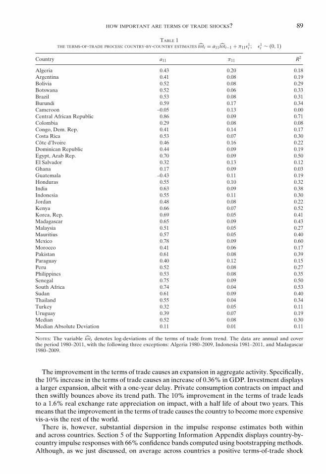
Table 1 displays country-specific estimates of Equation (3). The cross-country median of theestimated autocorrelation coefficient, a11, is 0.52. This means that terms-of-trade shocks vanishrelatively quickly, having a half life of about one year. The median unconditional standarddeviation of the innovation to the terms of trade, π11, is 0.08. The fit of the AR(1) process ismodest, as indicated by a median R2 of 0.30. Overall, the median estimate of the terms-of-tradeprocess is close to that obtained by Mendoza (1995), who uses terms-of-trade data from 1961to 1990 for a set of 23 poor and emerging countries, which has 16 countries in common withour 38-country panel. The cross-country estimate of the terms-of-trade process reported inMendoza (1995) is tott = 0.414 tott−1 + 0.1071ε1

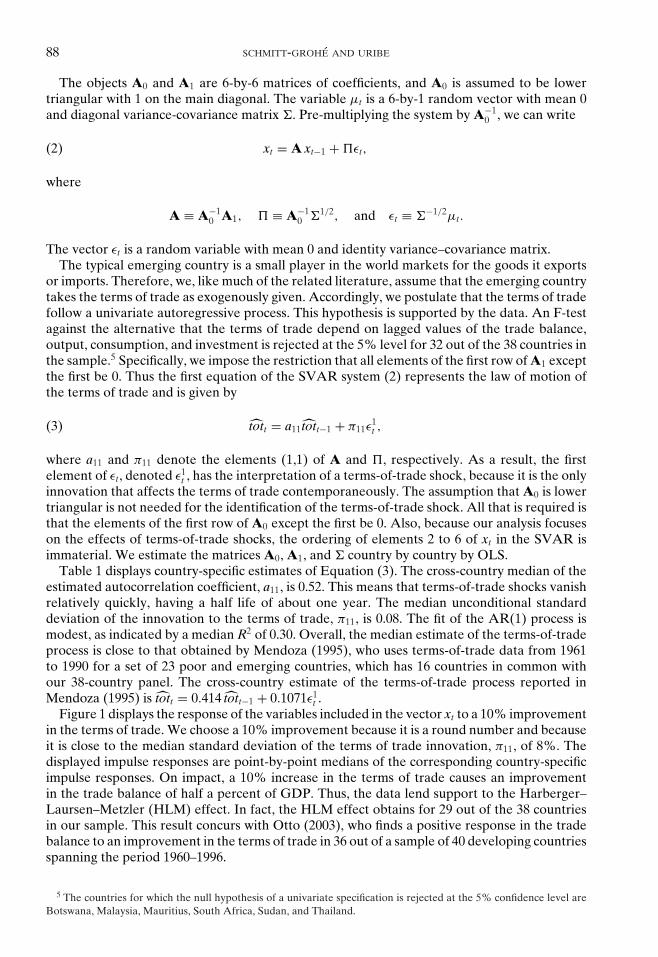
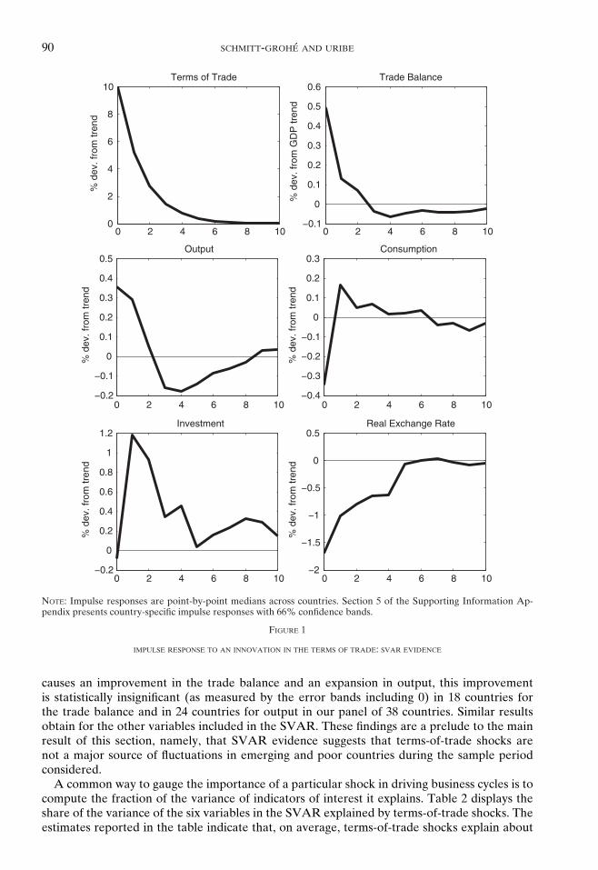
t .Figure 1 displays the response of the variables included in the vector xt to a 10% improvement

in the terms of trade. We choose a 10% improvement because it is a round number and becauseit is close to the median standard deviation of the terms of trade innovation, π11, of 8%. Thedisplayed impulse responses are point-by-point medians of the corresponding country-specificimpulse responses. On impact, a 10% increase in the terms of trade causes an improvementin the trade balance of half a percent of GDP. Thus, the data lend support to the Harberger–Laursen–Metzler (HLM) effect. In fact, the HLM effect obtains for 29 out of the 38 countriesin our sample. This result concurs with Otto (2003), who finds a positive response in the tradebalance to an improvement in the terms of trade in 36 out of a sample of 40 developing countriesspanning the period 1960–1996.

5 The countries for which the null hypothesis of a univariate specification is rejected at the 5% confidence level areBotswana, Malaysia, Mauritius, South Africa, Sudan, and Thailand.


TABLE 1THE TERMS-OF-TRADE PROCESS: COUNTRY-BY-COUNTRY ESTIMATES tott = a11 tott−1 + π11ε

1t ; ε1

t ∼ (0, 1)

Country a11 π11 R2

Algeria 0.43 0.20 0.18Argentina 0.41 0.08 0.19Bolivia 0.52 0.08 0.29Botswana 0.52 0.06 0.33Brazil 0.53 0.08 0.31Burundi 0.59 0.17 0.34Cameroon –0.05 0.13 0.00Central African Republic 0.86 0.09 0.71Colombia 0.29 0.08 0.08Congo, Dem. Rep. 0.41 0.14 0.17Costa Rica 0.53 0.07 0.30Cote d’Ivoire 0.46 0.16 0.22Dominican Republic 0.44 0.09 0.19Egypt, Arab Rep. 0.70 0.09 0.50El Salvador 0.32 0.13 0.12Ghana 0.17 0.09 0.03Guatemala –0.43 0.11 0.19Honduras 0.55 0.10 0.32India 0.63 0.09 0.38Indonesia 0.55 0.11 0.30Jordan 0.48 0.08 0.22Kenya 0.66 0.07 0.52Korea, Rep. 0.69 0.05 0.41Madagascar 0.65 0.09 0.43Malaysia 0.51 0.05 0.27Mauritius 0.57 0.05 0.40Mexico 0.78 0.09 0.60Morocco 0.41 0.06 0.17Pakistan 0.61 0.08 0.39Paraguay 0.40 0.12 0.15Peru 0.52 0.08 0.27Philippines 0.53 0.08 0.35Senegal 0.75 0.09 0.50South Africa 0.74 0.04 0.53Sudan 0.61 0.09 0.40Thailand 0.55 0.04 0.34Turkey 0.32 0.05 0.11Uruguay 0.39 0.07 0.19Median 0.52 0.08 0.30Median Absolute Deviation 0.11 0.01 0.11

NOTES: The variable tott denotes log-deviations of the terms of trade from trend. The data are annual and coverthe period 1980–2011, with the following three exceptions: Algeria 1980–2009, Indonesia 1981–2011, and Madagascar1980–2009.

The improvement in the terms of trade causes an expansion in aggregate activity. Specifically,the 10% increase in the terms of trade causes an increase of 0.36% in GDP. Investment displaysa larger expansion, albeit with a one-year delay. Private consumption contracts on impact andthen swiftly bounces above its trend path. The 10% improvement in the terms of trade leadsto a 1.6% real exchange rate appreciation on impact, with a half life of about two years. Thismeans that the improvement in the terms of trade causes the country to become more expensivevis-a-vis the rest of the world.

There is, however, substantial dispersion in the impulse response estimates both withinand across countries. Section 5 of the Supporting Information Appendix displays country-by-country impulse responses with 66% confidence bands computed using bootstrapping methods.Although, as we just discussed, on average across countries a positive terms-of-trade shock


0 2 4 6 8 100

2

4

6

8

10Terms of Trade

% d

ev. fr

om

tre

nd

0 2 4 6 8 10−0.1

0

0.1

0.2

0.3

0.4

0.5

0.6Trade Balance

% d

ev. fr

om

GD

P tre

nd

0 2 4 6 8 10−0.2

−0.1

0

0.1

0.2

0.3

0.4

0.5Output

% d

ev. fr

om

tre

nd

0 2 4 6 8 10−0.4

−0.3

−0.2

−0.1

0

0.1

0.2

0.3Consumption

% d

ev. fr

om

tre

nd

0 2 4 6 8 10−0.2

0

0.2

0.4

0.6

0.8

1

1.2Investment

% d

ev. fr

om

tre

nd

0 2 4 6 8 10−2

−1.5

−1

−0.5

0

0.5Real Exchange Rate

% d

ev. fr

om

tre

nd

NOTE: Impulse responses are point-by-point medians across countries. Section 5 of the Supporting Information Ap-pendix presents country-specific impulse responses with 66% confidence bands.

FIGURE 1

IMPULSE RESPONSE TO AN INNOVATION IN THE TERMS OF TRADE: SVAR EVIDENCE

causes an improvement in the trade balance and an expansion in output, this improvementis statistically insignificant (as measured by the error bands including 0) in 18 countries forthe trade balance and in 24 countries for output in our panel of 38 countries. Similar resultsobtain for the other variables included in the SVAR. These findings are a prelude to the mainresult of this section, namely, that SVAR evidence suggests that terms-of-trade shocks arenot a major source of fluctuations in emerging and poor countries during the sample periodconsidered.

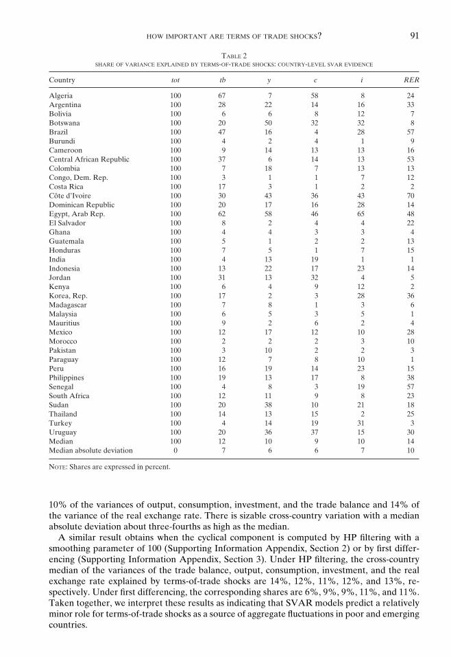
A common way to gauge the importance of a particular shock in driving business cycles is tocompute the fraction of the variance of indicators of interest it explains. Table 2 displays theshare of the variance of the six variables in the SVAR explained by terms-of-trade shocks. Theestimates reported in the table indicate that, on average, terms-of-trade shocks explain about


TABLE 2SHARE OF VARIANCE EXPLAINED BY TERMS-OF-TRADE SHOCKS: COUNTRY-LEVEL SVAR EVIDENCE

Country tot tb y c i RER

Algeria 100 67 7 58 8 24Argentina 100 28 22 14 16 33Bolivia 100 6 6 8 12 7Botswana 100 20 50 32 32 8Brazil 100 47 16 4 28 57Burundi 100 4 2 4 1 9Cameroon 100 9 14 13 13 16Central African Republic 100 37 6 14 13 53Colombia 100 7 18 7 13 13Congo, Dem. Rep. 100 3 1 1 7 12Costa Rica 100 17 3 1 2 2Cote d’Ivoire 100 30 43 36 43 70Dominican Republic 100 20 17 16 28 14Egypt, Arab Rep. 100 62 58 46 65 48El Salvador 100 8 2 4 4 22Ghana 100 4 4 3 3 4Guatemala 100 5 1 2 2 13Honduras 100 7 5 1 7 15India 100 4 13 19 1 1Indonesia 100 13 22 17 23 14Jordan 100 31 13 32 4 5Kenya 100 6 4 9 12 2Korea, Rep. 100 17 2 3 28 36Madagascar 100 7 8 1 3 6Malaysia 100 6 5 3 5 1Mauritius 100 9 2 6 2 4Mexico 100 12 17 12 10 28Morocco 100 2 2 2 3 10Pakistan 100 3 10 2 2 3Paraguay 100 12 7 8 10 1Peru 100 16 19 14 23 15Philippines 100 19 13 17 8 38Senegal 100 4 8 3 19 57South Africa 100 12 11 9 8 23Sudan 100 20 38 10 21 18Thailand 100 14 13 15 2 25Turkey 100 4 14 19 31 3Uruguay 100 20 36 37 15 30Median 100 12 10 9 10 14Median absolute deviation 0 7 6 6 7 10

NOTE: Shares are expressed in percent.

10% of the variances of output, consumption, investment, and the trade balance and 14% ofthe variance of the real exchange rate. There is sizable cross-country variation with a medianabsolute deviation about three-fourths as high as the median.

A similar result obtains when the cyclical component is computed by HP filtering with asmoothing parameter of 100 (Supporting Information Appendix, Section 2) or by first differ-encing (Supporting Information Appendix, Section 3). Under HP filtering, the cross-countrymedian of the variances of the trade balance, output, consumption, investment, and the realexchange rate explained by terms-of-trade shocks are 14%, 12%, 11%, 12%, and 13%, re-spectively. Under first differencing, the corresponding shares are 6%, 9%, 9%, 11%, and 11%.Taken together, we interpret these results as indicating that SVAR models predict a relativelyminor role for terms-of-trade shocks as a source of aggregate fluctuations in poor and emergingcountries.


TABLE 3SHARE OF VARIANCE EXPLAINED BY TERMS-OF-TRADE SHOCKS IN THE SVARS WITH INTEREST-RATE SPREADS

Specification tot s tb y c i RER

Baseline (no s) 100 – 12 10 9 10 14tot first 95 9 11 7 10 9 11s first 91 5 9 7 8 9 11

NOTE: Cross-country medians. Shares are expressed in percent. Section 6 of the Supporting Information Appendixprovides country-by-country results.

3. SVAR MODEL WITH INTEREST RATE SPREADS

A number of studies have shown that world interest rates play a role in driving businesscycles in emerging economies (among others, Neumeyer and Perri, 2005; Uribe and Yue, 2006;Garcıa-Cicco et al., 2010; Fernandez-Villaverde et al., 2011; Akinci, 2013). For the purpose ofthe present study, it is therefore of interest to ascertain the robustness of our results to expandingthe SVAR system to include some measure of the international cost of funds. In choosing sucha measure, we follow Akinci (2013), who shows that the Baa corporate bond spread is a morerelevant variable for emerging countries than less risky global interest-rate measures such asthe U.S. Federal Funds rate. The Baa corporate spread is defined as the difference betweenMoody’s seasoned Baa corporate bond yield and the federal funds rate (see the Appendix fordetails). As before, the SVAR system takes the form given in Equation (2), where the vector xt

now includes, in addition to the six variables considered in Section 2, the interest rate spread,denoted st and expressed in deviations from trend.

As in the related literature, we assume that the typical emerging economy takes the termsof trade and the U.S. interest-rate spread as exogenously given. We consider two identifica-tion schemes for the terms-of-trade shock. The first provides continuity with respect to theidentification strategy of Section 2. It assumes that terms-of-trade shocks affect the spreadcontemporaneously, but spread shocks affect the terms of trade only with a one-period lag.Formally, the first two equations of the SVAR model are assumed to take the form

[tott

st

]=

[a11 a12

a21 a22

] [tott−1

st−1

]+

[π11 0π21 π22

] [ε1

tε2

t

].(4)

As in the baseline identification, this scheme implies that the innovation to the terms-of-tradeequation, ε1

t , is the terms of trade shock. In addition, the innovation to the spread equation,ε2

t , has the interpretation of a spread shock. This ordering gives the terms of trade the highestchance to be an important source of fluctuations in domestic variables, as it attributes anyinnovation in the terms of trade to terms of trade shocks.

We also consider the alternative specification in which the terms of trade are placed secondin the SVAR, that is,

[st

tott

]=

[a11 a12

a21 a22

] [st−1

tott−1

]+

[π11 0π21 π22

] [ε1

tε2

t

].(5)

In this case, ε1t represents an interest-rate shock and ε2

t a terms-of-trade shock. We estimate theSVAR system by OLS equation by equation.

Table 3 displays cross-country medians of the estimated shares of the variances of the variablesincluded in the SVAR explained by terms-of-trade shocks. The results obtained under thebaseline SVAR specification are robust to including interest-rate spreads. Independently ofwhether the terms of trade are ordered first or second in the SVAR, their contribution toexplaining movements in key macroeconomic aggregates is around 10%. We interpret theresults presented here as further evidence that, when viewed through the lens of an SVAR


model, the contribution of terms-of-trade shocks to business-cycle fluctuations in emerging andpoor economies is modest. What do theoretical models have to say about this? This is the subjectof the following sections.

4. THE THEORETICAL MODEL

The model includes three sectors, an importable sector (the m sector), an exportable sector(the x sector), and a nontradable sector (the n sector). We refer to this framework as the MXNmodel. The structure of the model is similar to Mendoza (1995), with three generalizations.First, we assume that employment in the importable and exportable sectors is not fixed, butcan vary endogenously over the business cycle. This feature adds realism to the model, sincethese sectors represent a nonnegligible source of employment fluctuations. Second, we allowfor capital accumulation in the nontraded sector. This assumption is guided by the fact thatinvestment in the nontraded sector displays sizable volatility over the business cycle (McIntyre,2003). Third, we assume that investment goods are not fully imported and can have nontradedcomponents. Again, this modification is introduced to make the model more realistic, since alarge fraction of investment is made up of nontraded goods (Bems, 2008).

The reason why we choose to study this particular model is that, to a large extent, it has givenshape to the conventional wisdom that terms-of-trade shocks are a major driver of businesscycles. A natural question is why bother recomputing the predictions of this model. Our con-tribution in this regard is to parameterize the model in a way that we believe gives it a greaterchance to match the data. In particular, (i) we use country-specific estimates of the exogenousdriving forces, (ii) we estimate key structural parameters of the model country by country, and(iii) we place particular emphasis on expressing variables in the same units in the MXN andempirical models by using deflators defined in a consistent fashion.

4.1. Households. The model economy is populated by a large number of identical house-holds with preferences described by the utility function

E0

∞∑t=0

βtU (ct,hmt ,hx

t ,hnt ) ,(6)

where ct denotes consumption, hmt hours worked in the importable sector, hx

t hours worked inthe exportable sector, and hn

t hours worked in the nontradable sector. Households maximizetheir lifetime utility subject to the sequential budget constraint

ct + imt + ixt + int +�m(km

t+1 − kmt

) +�x(kx

t+1 − kxt

) +�n(kn

t+1 − knt

) + p τt dt

= p τt dt+1

1 + rt+ wm

t hmt + wx

t hxt + wn

t hnt + um

t kmt + ux

t kxt + un

t knt ,

where ijt , kj

t , wjt , and uj

t denote, respectively, gross investment, the capital stock, the real wage,and the rental rate of capital in sector j , for j = m, x,n with the superscripts m, x, and n de-noting the sector producing, respectively, importable, exportable, and nontraded goods. Thefunctions �j (·), j = m, x,n, introduce capital adjustment costs and are assumed to be nonneg-ative and convex and to satisfy �j (0) = �′

j (0) = 0. The variable p τt denotes the relative priceof the tradable composite goods in terms of final goods (to be formally defined below), dt de-notes the stock of debt in period t, expressed in units of the tradable composite goods, and rt

denotes the interest rate on debt held from period t to t + 1. Consumption, investment, wages,rental rates, debt, and capital adjustment costs are all expressed in units of final goods.

The capital stocks obey the familiar laws of motion

kmt+1 = (1 − δ)km

t + imt ,(7)


kxt+1 = (1 − δ)kx

t + ixt ,(8)

and

knt+1 = (1 − δ)kn

t + int .(9)

Using these laws of motion to eliminate imt , ixt , and int from the household’s budget constraintand letting λtβ

t denote the Lagrange multiplier associated with the resulting budget constraint,we have that the first-order optimality conditions with respect to ct, hm

t , hxt , hn

t , dt+1, kmt+1, kx

t+1,and kn

t+1 are, respectively,

U1 (ct,hmt ,hx

t ,hnt ) = λt(10)

−U2 (ct,hmt ,hx

t ,hnt ) = λtw

mt(11)

−U3 (ct,hmt ,hx

t ,hnt ) = λtw

xt(12)

−U4 (ct,hmt ,hx

t ,hnt ) = λtw

nt(13)

λt p τt = β(1 + rt)Etλt+1 p τt+1(14)

λt[1 +�′

m

(km

t+1 − kmt

)] = βEtλt+1[um

t+1 + 1 − δ+�′m

(km

t+2 − kmt+1

)](15)

λt[1 +�′

x

(kx

t+1 − kxt

)] = βEtλt+1[ux

t+1 + 1 − δ+�′x

(kx

t+2 − kxt+1

)](16)

λt[1 +�′

n

(kn

t+1 − knt

)] = βEtλt+1[un

t+1 + 1 − δ+�′n

(kn

t+2 − knt+1

)].(17)

It is clear from these expressions that the rates of return on capital may display cyclical differ-ences across sectors but are equalized in the steady state. By contrast, sectoral wage differencesmay persist even in the steady state.

4.2. Firms Producing Final Goods. Final goods are produced using nontradable goods and acomposite of tradable goods via the technology B(aτt , an

t ), where aτt denotes domestic absorptionof the tradable composite goods, and an

t denotes domestic absorption of nontraded goods. Theaggregator function B(·, ·) is assumed to be increasing, concave, and homogeneous of degree1. Final goods are sold to households, which then allocate them to consumption or investmentpurposes. Producers of final goods behave competitively. Their profits are given by

B (aτt , ant ) − p τt aτt − p n

t ant ,

where p nt denotes the relative price of nontradable goods in terms of final goods. The firm’s

profit maximization conditions are

B1 (aτt , ant ) = p τt(18)


and

B2 (aτt , ant ) = p n

t .(19)

These expressions define the domestic demand functions for nontradables and for the tradablecomposite goods.

4.3. Firms Producing the Tradable Composite Good. The tradable composite goods are pro-duced using importable and exportable goods as intermediate inputs, via the technology

aτt = A (amt , ax

t ) ,(20)

where amt and ax

t denote the domestic absorptions of importable and exportable goods, respec-tively. The aggregator function A(·, ·) is increasing, concave, and linearly homogeneous. Profitsare given by

p τt A (amt , ax

t ) − p mt am

t − p xt ax

t ,

where p mt denotes the relative price of importable goods in terms of final goods and p x

t denotesthe relative price of exportable goods in terms of final goods. Firms in this sector are assumedto behave competitively in intermediate and final goods markets. Then, profit maximizationimplies that

p τt A1 (amt , ax

t ) = p mt(21)

and

p τt A2 (amt , ax

t ) = p xt .(22)

These two expressions represent the domestic demand functions for importable and exportablegoods.

4.4. Firms Producing Importable, Exportable, and Nontradable Goods. Importable, ex-portable, and nontradable goods are produced with capital and labor via the technologies

ymt = AmF m (km

t ,hmt )(23)

yxt = AxF x (kx

t ,hxt ) ,(24)

and

ynt = AnF n (kn

t ,hnt ) ,(25)

where yjt and Aj denote, respectively, output and a productivity factor in sector j = m, x,n.

The production functions F j (·, ·), j = m, x,n, are assumed to be increasing in both arguments,concave, and homogeneous of degree 1. Profits of firms producing exportable, importable, ornontraded goods are given by

p jt F j

(kj

t ,hjt

)− w

jt hj

t − ujt kj

t ,


for j = m, x,n. Firms are assumed to behave competitively in product and factor markets. Then,the first-order profit maximization conditions are

p mt AmF m

1 (kmt ,hm

t ) = umt(26)

p mt AmF m

2 (kmt ,hm

t ) = wmt(27)

p xt AxF x

1 (kxt ,hx

t ) = uxt(28)

p xt AxF x

2 (kxt ,hx

t ) = wxt(29)

p nt AnF n

1 (knt ,hn

t ) = unt(30)

p nt AnF n

2 (knt ,hn

t ) = wnt .(31)

These efficiency conditions represent the sectoral demand functions for capital and labor.Together with the assumption of linear homogeneity of the production technologies, they implythat firms make zero profits at all times.

4.5. Competitive Equilibrium. In equilibrium the demand for final goods must equal thesupply of this type of goods:

ct + imt + ixt + int +�m(km

t+1 − kmt

) +�x(kx

t+1 − kxt

) +�n(kn

t+1 − knt

) = B (aτt , ant ) .(32)

Also, the demand for nontradables must equal the production of nontradables:

ant = yn

t .(33)

Imports, denoted mt, are defined as the difference between the domestic absorption of im-portables, am

t , and importable output, ymt , or

mt = p mt (am

t − ymt ) .(34)

The price of importables appears on the right-hand side of this definition because mt is expressedin units of final goods, whereas ym

t and amt are expressed in units of importable goods. Similarly,

exports, denoted xt, are given by the difference between exportable output, yxt , and the domestic

absorption of exportables, axt ,

xt = p xt (yx

t − axt ) .(35)

Like imports, exports are measured in terms of final goods.Combining the above two definitions, the household’s budget constraint, and the definitions

of profits in the final- and intermediate-good markets and taking into account that firms makezero profits at all times yields the following economy-wide resource constraint:

p τtdt+1

1 + rt= p τt dt + mt − xt.(36)


To ensure a stationary equilibrium process for external debt, we follow Schmitt-Grohe andUribe (2003) and assume that the country interest rate is debt elastic:

rt = r∗ + st + p(dt+1),(37)

where r∗ denotes the risk-free world interest rate, st denotes the global component of theinterest-rate spread, and p(d) denotes the domestic component of the interest-rate spread. Weassume that p(d) = 0 and p ′(d) > 0, for some constant d.

Given the definition of the terms of trade as the relative price of exportable goods in termsof importable goods, we have that

tott = p xt

p mt.(38)

As in the empirical analysis of Section 3, we assume that the country is small in internationalproduct and asset markets and therefore takes the evolution of the terms of trade, tott, andthe global component of the interest-rate spread, st, as exogenously given. Also in line withthe empirical analysis of Section 3, we assume that tott and st follow the joint law of motiongiven in Equation (4), with tott ≡ ln(tott/tot), st ≡ st − s, and tot and s denoting the deterministicsteady-state values of tott and st, respectively.

As explained earlier, the real exchange rate is defined as the ratio of the foreign consumerprice index to the domestic consumer price index. Formally,

RERt = EtP∗t

Pt,

where Et denotes the nominal exchange rate, defined as the domestic-currency price of one unitof foreign currency, P∗

t denotes the foreign price of consumption, and Pt denotes the domesticprice of consumption. Dividing the numerator and denominator by the domestic-currency priceof the tradable composite goods, denoted Pτ

t , yields RERt = (EtP∗t /P

τt )/(Pt/Pτ

t ). We assumethat the law of one price holds for importable and exportable goods and that the technology foraggregating importables and exportables into the tradable composite goods, A(·, ·), is commonacross countries. Then, the law of one price must also hold for the tradable composite goods,that is, EtPτ∗

t = Pτt , where Pτ∗

t denotes the foreign price of the tradable composite goods. ThisyieldsRERt = (P∗

t /Pτ∗t )/(Pt/Pτ

t ). We assume that the terms-of-trade shocks that are relevant toour small open economy do not affect the relative price of the tradable composite goods in termsof consumption goods in the rest of the world. We therefore assume that P∗

t /Pτ∗t is constant.

Without loss of generality, we normalize P∗t /P

τ∗t to unity. Finally, noting that p τt ≡ Pτ

t /Pt, wehave

RERt = p τt ,(39)

which says that the real exchange rate equals the relative price of the tradable composite goodsin terms of final goods. It can be shown that there is a one-to-one negative relationship betweenp τt and p n

t . That is, the tradable goods becomes more expensive relative to the final consumptiongoods if and only if the nontradable goods becomes cheaper relative to the final consumptiongoods. This means that we can express the real exchange rate as a decreasing function of therelative price of nontradables, RERt = γ(p n

t ), γ′ < 0.A competitive equilibrium is then a set of 33 processes km

t+1, imt , kxt+1, ixt , kn

t+1, int , ct, hmt , hx

t ,hn

t , λt, wmt , wx

t , wnt , p τt , RERt, rt, um

t , uxt , un

t , amt , ax

t , aτt , p mt , p x

t , ant , p n

t , ymt , yx

t , ynt , mt, xt, and

dt+1, satisfying Equations (7) to (39), given initial conditions km0 , kx

0, kn0 , and d0, and the joint

stochastic process for tott and st given in Equation (4).


4.6. Observables. In the present model, ct denotes consumption expressed in units of fi-nal (consumption) goods. GDP, investment, and the trade balance expressed in units of finalconsumption goods, denoted yt, it, and tbt, respectively, are given by

yt = p mt ym

t + p xt yx

t + p nt yn

t ,(40)

it = imt + ixt + int ,

and

tbt = xt − mt.

The data used in the empirical analysis of Section 2, however, are not expressed in terms offinal consumption goods. A meaningful comparison of the model predictions with data requiresexpressing theoretical and empirical variables in the same units. In the SVAR analysis ofSection 2, data on GDP, consumption, investment, and the trade balance are deflated by aPaasche GDP deflator. In this section we derive the corresponding theoretical counterparts. Inthe theoretical model, GDP at current prices is given by

Pmt ym

t + Pxt yx

t + Pnt yn

t ,

where Pit denotes the nominal price of goods i in period t, for i = m, x,n. The data source (WDI)

uses a Paasche index for the GDP deflator, defined as the ratio of current-price to constant-priceGDP. That is, the GDP deflator in period t is given by

Pmt ym

t + Pxt yx

t + Pnt yn

t

Pm0 ym

t + Px0 yx

t + Pn0 yn

t,

where t = 0 indicates the base year. Real GDP is nominal GDP divided by the GDP deflator,that is,

Pm0 ym

t + Px0 yx

t + Pn0 yn

t .

The nominal prices in the base year, Pm0 , Px

0 , and Pn0 , as well as all other nominal prices in period

0 are indices without a real unit attached. Therefore, without loss of generality we can set onenominal base price arbitrarily. Thus we set the nominal price of consumption in period 0 equalto 1, P0 = 1. This means that Pi

0 = p i0 for i = m, x,n (recall that p i

t is the relative price of goodsi in terms of final consumption goods for i = m, x,n). Real output in period t is then given by

p m0 ym

t + p x0yx

t + p n0 yn

t .

Finally, we must take a stance on what the state of the economy looked like in the base period.We assume that in the base period the economy was in the deterministic steady state, so thatp i

0 = p i for i = m, x,n. Then, the theoretical counterpart of the observed measure of real GDP,which we denote by yo

t , is given by6

yot = p mym

t + p xyxt + p nyn

t .(41)

6 In the SVAR, real variables are expressed in per capita terms. In the theoretical model, there is no populationgrowth, so real GDP and real GDP per capita are the same.


Similarly, the theoretical counterpart of real consumption is the ratio of nominal consumption,Ptct, to the GDP deflator, or

cot ≡ Ptct

Pm0 ym

t + Px0 yx

t + Pn0 yn

t

Pmt ym

t + Pxt yx

t + Pnt yn

t.

Recalling that p it ≡ Pi

t/Pt and that Pi0 = p i for i = m, x,n, we can write the theoretical counter-

part of observed real consumption as

cot = ct

p mymt + p xyx

t + p nynt

p mt ym

t + p xt yx

t + p nt yn

t.

The theoretical counterparts of observed real investment and the trade balance can be obtainedin a similar fashion, that is,

iot = itp mym

t + p xyxt + p nyn

t

p mt ym

t + p xt yx

t + p nt yn

t

and

tbot = tbt

p mymt + p xyx

t + p nynt

p mt ym

t + p xt yx

t + p nt yn

t.

When comparing the predictions of the theoretical model to the data, we use predictionsregarding yo

t , cot , iot , and tbo

t as opposed to the corresponding measures in terms of final goods, yt,ct, it, and tbt. This ensures congruency of the data with the model in the definition of variables. Aswe will see in Section 6, it makes a significant difference for the share of variance explained byterms-of-trade shocks whether one uses data-consistent measures of macroeconomic indicatorsor measures expressed in terms of final goods.

4.7. Functional Forms. We assume that the period utility function displays constant relativerisk aversion (CRRA) in a quasi-linear composite of consumption and labor:

U(c,hm,hx,hn) = [c − G(hm,hx,hn)]1−σ − 11 − σ

,

where

G(hm,hx,hn) = (hm)ωm

ωm+ (hx)ωx

ωx+ (hn)ωn

ωn,

with σ, ωm, ωx, ωn > 0. This specification implies that sectoral labor supplies are wealth inelastic.The technologies for producing importables, exportables, and nontradables are all assumed

to be Cobb–Douglas,

F m(km,hm) = (km)αm (hm)1−αm ,

F x(kx,hx) = (kx)αx (hx)1−αx ,

and

F n(kn,hn) = (kn)αn (hn)1−αn ,


TABLE 4CALIBRATION OF THE MXN MODEL

Calibrated Structural Parameters

σ δ r∗ + s αm, αx αn ωm, ωx, ωn μmx μτn tot Am,An β

2 0.1 0.11 0.35 0.25 1.455 1 0.5 1 1 1/(1 + r∗ + s)

Moment Restrictions

sn sx stbpmym

pxyx

0.5 0.2 0.01 1

Implied Structural Parameter Values

χm χτ d Ax β

0.8980 0.4360 0.0078 1 0.9009

Estimated Parameters

φm φx φn ψ a11 a12 a21 a22 π11 π21 π22* * * * ** ** ** ** ** ** **

NOTE: sn ≡ pnyn/y, sx ≡ x/y, and stb ≡ (x − m)/y, where y ≡ pmym + pxyx + pnyn .*Country-specific estimates are presented in Table 5. **Country-specific estimates are given in Section 6 of the Sup-porting Information Appendix.

where αm, αx, αn ∈ (0, 1). We assume that the Armington aggregators used in the production ofthe tradable composite goods and the final goods take CES forms, that is,

A (amt , ax

t ) =[χm (am

t )1− 1μmx + (1 − χm) (ax

t )1− 1μmx

] 11− 1

μmx

B(aτt , ant ) =

[χτ (aτt )1− 1

μτn + (1 − χτ) (ant )1− 1

μτn

] 11− 1

μτn ,

with χm, χτ ∈ (0, 1) and μmx, μτn > 0. The specification of the interest-rate premium and thecapital adjustment costs are, respectively,

p(d) = ψ(

ed−d − 1)

and

�j (x) = φj

2x2,

with ψ, φj > 0, for j = m, x,n.

5. CALIBRATION, ESTIMATION, AND IMPULSE RESPONSES

The MXN model is medium scale in size and lies at the intersection of trade and business-cycleanalysis. The characterization of the steady state is complex—even numerically. The calibrationof the model inherits this complexity.

Tables 4 and 5 summarize the calibration and estimation results. The time unit is meantto be a year. We denote the steady-state value of a variable by dropping the time subscript.The equilibrium conditions (7)–(39) evaluated at the steady state and adopting the assumedfunctional forms represent a system of 33 equations in 52 unknowns, namely, the 33 endoge-nous variables listed in the definition of equilibrium given in Subsection 4.5 and 19 structuralparameters, namely, Am, Ax, An, δ, ωm, ωx, ωn, β, χm, μmx, χτ, μτn, αm, αx, αn, r∗ + s, d, tot, and


TABLE 5COUNTRY-SPECIFIC ESTIMATES OF THE CAPITAL ADJUSTMENT COST PARAMETERS AND THE DEBT ELASTICITY OF THE INTEREST

RATE

Country φm φx φn ψ

Algeria 73.26 79.24 73.60 0.72Argentina 0.04 10.02 8.80 57.57Bolivia 76.87 77.26 76.42 60.19Botswana 0.13 12.74 0.13 66.79Brazil 77.89 54.61 75.71 71.67Burundi 0.18 2.97 5.09 0.01Cameroon 0.81 67.35 78.44 42.29Central African Republic 1.71 73.39 79.72 50.12Colombia 12.05 0.97 1.82 5.31Congo, Dem. Rep. 31.38 79.26 4.23 22.35Costa Rica 45.07 33.13 78.24 0.02Cote d’Ivoire 47.36 78.77 69.61 0.31Dominican Republic 0.05 36.93 0.30 19.62Egypt, Arab Rep. 39.29 79.06 36.60 0.03El Salvador 77.66 2.18 79.87 2.09Ghana 76.86 70.43 79.65 0.05Guatemala 70.20 77.67 45.93 0.01Honduras 3.62 2.44 9.46 0.00India 51.44 12.37 75.14 0.88Indonesia 8.96 79.52 0.45 78.83Jordan 33.99 78.59 75.82 0.43Kenya 38.48 79.10 63.71 0.03Korea, Rep. 5.50 49.18 68.05 9.65Madagascar 17.43 22.33 0.91 0.00Malaysia 48.49 66.90 13.40 0.30Mauritius 30.50 74.04 68.71 0.03Mexico 78.24 46.33 68.65 0.29Morocco 75.85 78.07 68.23 78.82Pakistan 54.50 79.63 77.57 0.02Paraguay 77.48 31.66 79.08 6.91Peru 78.73 74.39 37.65 5.49Philippines 79.20 7.30 70.09 0.06Senegal 13.59 79.42 20.80 0.01South Africa 42.66 79.77 55.58 0.03Sudan 41.02 35.78 31.75 0.02Thailand 74.98 37.47 38.05 0.03Turkey 52.55 1.02 77.12 3.66Uruguay 68.18 78.29 74.65 78.17Median 43.87 67.13 68.14 0.58Median absolute deviation 31.46 12.51 11.54 0.57

σ. (The structural parameters ψ , aij , πij , for i, j = 1, 2, and φj , for j = m, x,n do not appearin the steady-state system. We will address the values assigned to these parameters shortly.)Therefore, we must add 19 calibration restrictions (which we enumerate in parenthesis). (1) Weset σ = 2, which is a common value in business-cycle analysis. (2)–(4) ωm = ωx = ωn = 1.455.This value implies a sectoral Frisch elasticity of labor supply of 2.2, which is the number assumedin the one-sector model studied in Mendoza (1991). Lacking sector-level information about thiselasticity, we assume the same value in the three sectors. (5) We assume a depreciation rate ofphysical capital of δ = 0.1, which is a standard value. (6) r∗ + s = 0.11 (the split of this valuebetween r∗ and s is immaterial). This value is taken from Uribe and Yue (2006) and reflectsthe relatively high average interest rate faced by poor and emerging countries in world finan-cial markets. (7) μmx = 1. There is a vast literature on estimating the elasticity of substitutionbetween exportable and importable goods, μmx. One branch of this literature uses aggregate


data at quarterly frequency and estimates μmx in the context of open-economy DSGE models.This body of work typically estimates μmx to be below unity. For instance, Corsetti et al. (2008),Gust et al. (2009), and Justiniano and Preston (2010) all estimate μ to lie between 0.8 and 0.86.Miyamoto and Nguyen (2014) estimate μmx to be 0.4. A second branch of the literature infersthe value of μmx from trade liberalization episodes using average changes in quantities andprices observed over periods of 5–10 years. This approach typically yields values of μmx greaterthan 1, in the neighborhood of 1.5 (see, for example, Whalley, 1985). It is intuitive that studiesbased on low frequency data deliver values of μmx higher than studies based on quarterly data.It is natural to expect that agents can adjust more fully to relative-price changes in the longrun than in the short run. Because SVAR analysis Section 2 uses annual data, it is sensible toadopt a value of μmx in between those stemming from the two aforementioned bodies of work.Accordingly, we set μmx equal to 1. (8) tot = 1. (9) Am = 1. (10) An = 1. (11) β = 1/(1 + r∗ + s).Restrictions (8)–(11) are normalizations, with (11) ensuring that the steady-state level of debtcoincides with the parameter d. (12) The average of the ratio of value added exports to GDPacross poor and emerging countries computed using data from the OECD’s TiVA databaseis 20%. Therefore, we impose x/(p mym + p xyx + p nyn) = 0.2. (13) In our sample of 38 coun-tries, the average trade balance-to-GDP ratio is 1%, or (x − m)/(p mym + p xyx + p nyn) = 0.01.(14) Na (2015) estimates an average labor share for emerging countries of 70%, so we im-pose (wmhm + wxhx + wnhn)/(p mym + p xyx + p nyn) = 0.7. (15) It is generally assumed that inemerging and poor countries the nontraded sector is more labor intensive than the exportor import producing sectors. For instance, Uribe (1997), based on Argentine data, calcu-lates the labor share in the nontraded sector to be 0.75. We follow this calibration and im-pose the restriction wnhn/(p nyn) = 0.75. (16) Lacking cross-country evidence on labor sharesin the import and export sectors, we assume that the importable and exportable sectors areequally labor intensive; that is, we impose wmhm/(p mym) = wxhx/(p xyx). (17) We follow theusual practice of proxying the share of nontraded output in total output by the observedshare of the service sector in GDP. Using data from UNCTAD’s Handbook of Statisticson sectoral GDP for poor and emerging countries over the period 1995 to 2012, we obtainan average share of services in GDP of slightly above 50%. Thus, we impose the restrictionp nyn/(p mym + p xyx + p nyn) = 0.5. (18) Using data from UNCTAD, we estimate that in emerg-ing and poor countries the exportable and importable sectors are of about the same size. There-fore, we impose the restriction p xyx = p mym. (19) Finally, Akinci (2011) surveys the literatureon estimates of the elasticity of substitution between tradables and nontradables in emergingand poor countries and arrives at a value close to 0.5. Thus we set μτn = 0.5. This completesthe calibration strategy of the 19 parameters appearing in the set of steady-state equilibriumconditions.

The parameters aij , πij for i, j = 1, 2, φj , for j = m, x,n, and ψ do not appear in the steady-state equilibrium conditions but play a role in the equilibrium dynamics. We assign values to aij

and πij for i, j = 1, 2 country by country using the econometric estimates presented in Section 6of the Supporting Information Appendix. We use a partial information method to estimatethe capital adjustment cost parameters, φm, φx, φn, and the parameter ψ governing the debtelasticity of the country premium. Specifically, we set these parameters to minimize a weighteddifference between the impulse responses to terms-of-trade and interest-rate-spread shocks ofoutput, consumption, investment, the trade balance, and the real exchange rate implied by theSVAR and MXN models. We consider the first five years of each impulse response functionand use as weights the reciprocal of the width of the 66% confidence interval associated withthe SVAR impulse responses. Formally, letting � ≡ [φm φx φn ψ], we set � as the solution tothe problem

min�

∑h=tot,s

4∑i=0

∑j=yo,co,io,tbo,RER

∣∣∣IRSVARhij − IRMXN

hij (�)∣∣∣

�hij,


where IRSVARhij and IRMXN

hij (�) denote the impulse response of variable ji periods after a shock himplied by the SVAR and MXN models, respectively, and �hij denotes the width of the 66%confidence band associated with IRSVAR

hij . We perform this estimation country by country.Table 5 displays the estimated parameters. There is substantial cross-country dispersion in

the estimated parameter values, especially for φm andψ , which have median absolute deviationsalmost as large as the estimated medians themselves. This suggests that the strategy of estimatingparameters country by country is preferred to the standard practice of one parameterizationfor all countries.

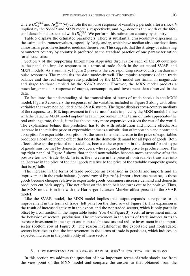
Section 7 of the Supporting Information Appendix displays for each of the 38 countriesin the panel the impulse responses to a terms-of-trade shock in the estimated SVAR andMXN models. As a summary, Figure 2 presents the corresponding cross-country median im-pulse responses. The model fits the data modestly well. The impulse responses of the tradebalance and the real exchange rate predicted by the MXN model are similar in magnitudeand shape to those implied by the SVAR model. However, the MXN model predicts amuch larger median response of output, consumption, and investment than observed in thedata.

To facilitate the understanding of the transmission of terms-of-trade shocks in the MXNmodel, Figure 3 considers the responses of the variables included in Figure 2 along with othervariables that were not included in the SVAR system. The figure displays cross-country mediansof the response to a 10% improvement in the terms of trade implied by the MXN model. In linewith the data, the MXN model implies that an improvement in the terms of trade appreciates thereal exchange rate, that is, it makes the country more expensive vis-a-vis the rest of the world.The explanation behind this prediction has to do with substitution and income effects. Anincrease in the relative price of exportables induces a substitution of importable and nontradedabsorption for exportable absorption. At the same time, the increase in the price of exportablesproduces a positive income effect that boosts the domestic demand for all types of goods. Botheffects drive up the price of nontradables, because the expansion in the demand for this typeof goods must be met by domestic producers, who require a higher price to produce more. Thetop right panel of Figure 3 shows that indeed nontradables become more expensive after thepositive terms-of-trade shock. In turn, the increase in the price of nontradables translates intoan increase in the price of the final goods relative to the price of the tradable composite goods;that is, p τt falls.

The increase in the terms of trade produces an expansion in exports and imports and animprovement in the trade balance (second row of Figure 3). Imports increase because, as thesegoods become cheaper relative to exportable goods, consumers increase demand and domesticproducers cut back supply. The net effect on the trade balance turns out to be positive. Thus,the MXN model is in line with the Harberger–Laursen–Metzler effect present in the SVARmodel.

Like the SVAR model, the MXN model implies that output expands in response to animprovement in the terms of trade (left panel on the third row of Figure 3). This expansion isthe result of increased activity in the export and the nontraded sectors, which is only partiallyoffset by a contraction in the importable sector (row 4 of Figure 3). Sectoral investment mimicsthe behavior of sectoral production. The improvement in the terms of trade induces firms toincrease investment in the export and nontradable sectors and reduce investment in the importsector (bottom row of Figure 3). The reason investment in the exportable and nontradablesectors increases is that the improvement in the terms of trade is persistent, which induces anexpected increase in the profitability of these sectors.

6. HOW IMPORTANT ARE TERMS-OF-TRADE SHOCKS? THEORETICAL PREDICTIONS

In this section we address the question of how important terms-of-trade shocks are fromthe view point of the MXN model and compare the answer to that obtained from the


0 2 4 6 8 10−5

0

5

10Terms of Trade

0 2 4 6 8 10−0.2

−0.15

−0.1

−0.05

0Spread

0 2 4 6 8 10−0.5

0

0.5

1Trade Balance

0 2 4 6 8 10−0.5

0

0.5

1

1.5

2Output

0 2 4 6 8 10−0.5

0

0.5

1Consumption

0 2 4 6 8 10−2

−1

0

1

2

3Investment

0 2 4 6 8 10−2

−1.5

−1

−0.5

0

0.5Real Exchange Rate

: SVAR model; —o—o—o—: MXN model

FIGURE 2

MEDIAN RESPONSE TO A 10% TERMS-OF-TRADE SHOCK: DATA VERSUS MODEL

SVAR model. We compute the share of the variance of output explained by terms-of-tradeshocks as the ratio of the variance of output conditional on terms-of-trade shocks impliedby the MXN model to the unconditional variance of output implied by the SVAR model ofSection 3.

The first two columns of Table 6 show that, like the SVAR model of Section 3, the MXNmodel assigns a small role to terms-of-trade shocks in explaining the variance of output. Inboth the SVAR and MXN models, the cross-country median of the share of the variance of


0 5 10−5

0

5

10Terms of Trade

0 5 10−2

−1.5

−1

−0.5

0Real Exchange Rate

0 5 100

0.5

1

1.5

2Rel Price of Nontradables

0 5 10−0.5

0

0.5

1Trade Balance

0 5 100

5

10

15Imports

0 5 100

5

10

15

20Exports

0 5 100

0.5

1

1.5

2Output

0 5 10

0.7

0.8

0.9

1Consumption

0 5 100

1

2

3Investment

0 5 10−3

−2

−1

0

1Output in Import Sector

0 5 100

2

4

6Output in Export Sector

0 5 100.5

1

1.5

2Output in Nontraded Sector

0 5 10−15

−10

−5

0

5Investment in Import Sector

0 5 10−10

0

10

20Investment in Export Sector

0 5 100

2

4

6Investment in Nontraded Sector

NOTE: All variables with the exception of the trade balance are expressed in percent deviations from steady state. Thetrade balance is expressed in level deviations from steady state in percent of steady-state output. Impulse responses arecross-country medians. For each country, impulse responses are produced using the country specific estimates of φm,φx, φn , ψ , aij , and πij , for i, j = 1, 2.

FIGURE 3

RESPONSE OF THE MXN ECONOMY TO A 10% TERMS-OF-TRADE SHOCK


TABLE 6SHARE OF OUTPUT VARIANCE EXPLAINED BY TERMS-OF-TRADE SHOCKS: SVAR VERSUS MXN MODEL

MXN Model

Paasche GDP Deflator Units of Final GoodsSVAR Model (yo

t ) (yt)

Median 7.1 9.2 27.4MAD 5.8 6.1 16.8

NOTE: MAD stands for median absolute deviation. Medians and median absolute deviations are taken over the 38countries in the panel. Variance shares are computed as the ratio of variances of output conditional on terms-of-tradeshocks to the unconditional variance of output implied by the SVAR model of Section 3.

output explained by terms-of-trade disturbances is less than 10%. This result is at odds with thefindings in the related literature that uses theoretical models similar to the MXN model studiedhere, which attributes a major role to terms-of-trade disturbances as drivers of business cyclesin poor and emerging countries.

What could account for this discrepancy? As discussed earlier, our estimate of the terms-of-trade process is quite similar to those used in related studies, suggesting that this is notthe source of the discrepancy. The third column of Table 6 suggests one possible explanationfor the discrepancy between the small role of terms of trade documented here and the largerole that is conventionally assigned to this source of uncertainty in the context of theoreticalmodels similar to the MXN model. As mentioned in Subsection 4.6, the empirical measureof output in the WDI database is the result of deflating nominal output by a Paasche GDPdeflator. Its counterpart in the theoretical model is output measured at constant prices, yo

t ,as defined in Equation (41). Conventionally, however, theoretical studies measure output inunits of final goods, yt, as defined in Equation (40). Table 6 shows that the importance ofterms-of-trade shocks is quite sensitive to the specific deflator used to define real output in thetheoretical model. When output is measured in units of final goods, the MXN model predictsthat terms-of-trade shocks explain on average almost 30% of the variance of output, whichimplies a sizable role for the terms of trade as a source of business-cycle fluctuations. However,this conclusion would be misplaced, since it is based on a number that lacks the interpretationof a variance share. To see this, recall that the denominator of this variance share (i.e., theunconditional variance of output implied by the SVAR model) is computed using a measureof output deflated by a Paasche GDP deflator, whereas the numerator is computed using ameasure of output expressed in units of current final goods.

The reason the variance of output conditional on terms-of-trade shocks is predicted to behigher when output is measured in units of final goods than when it is deflated by a PaascheGDP deflator is as follows. Recall that when output is deflated by the Paasche GDP deflator,quantities are weighted by time invariant prices. By contrast, when output is measured inunits of (current) final goods, quantities are weighted by time-varying prices. Depending onthe correlation structure of prices and quantities, the two measures can, in principle, give riseto different results. Consider a simple example of an economy that produces only exportablegoods and consumes only importable goods. In this case, we have that yo

t = yxt and yt = p x

t + yxt ,

where a hat denotes log-deviation from the steady state. Then we have that var(yot ) = var(yx

t ),whereas var(yt) = var(p x

t ) + var(yxt ) + 2cov(p x

t , yxt ). The covariance between p x

t and yxt has the

same sign as the covariance between the terms of trade and p xt , since in this economy one can

show that p xt depends only on and is increasing in the terms of trade. Also, the production of

exportables increases with the terms of trade. This implies that the variance of yot conditional on

terms-of-trade shocks is smaller than that of yt. In words, since prices and quantities move in thesame direction in response to terms-of-trade shocks, the conditional variance of output is higherwhen the quantity of exportables is multiplied by current prices than when it is multiplied bysteady-state prices. To the extent that the effects of terms-of-trade shocks in the MXN model


0 10 20 30 40 50 600

10

20

30

40

50

60

Alg

Arg

Bol Bot

Bra

Bur

Cam

Cen

Col

Con

Cos

Cot

Dom

Egy

El

Gha

Gua

Hon

Ind

Ind

Jor

Ken

Kor

Mad

Mal

Mau

Mex

Mor

Pak

Par

Per

Phi

Sen

Sou

Sud

Tha

Tur Uru

45o

SVAR Model

MX

N M

odel

NOTE: Variance shares are expressed in percent.

FIGURE 4

VARIANCE OF OUTPUT EXPLAINED BY TERMS-OF-TRADE SHOCKS: SVAR MODEL VERSUS MXN MODEL

are dominated by the dynamics of the exportable sector, the intuition derived from the simpleeconomy will carry over.

7. THE TERMS-OF-TRADE DISCONNECT

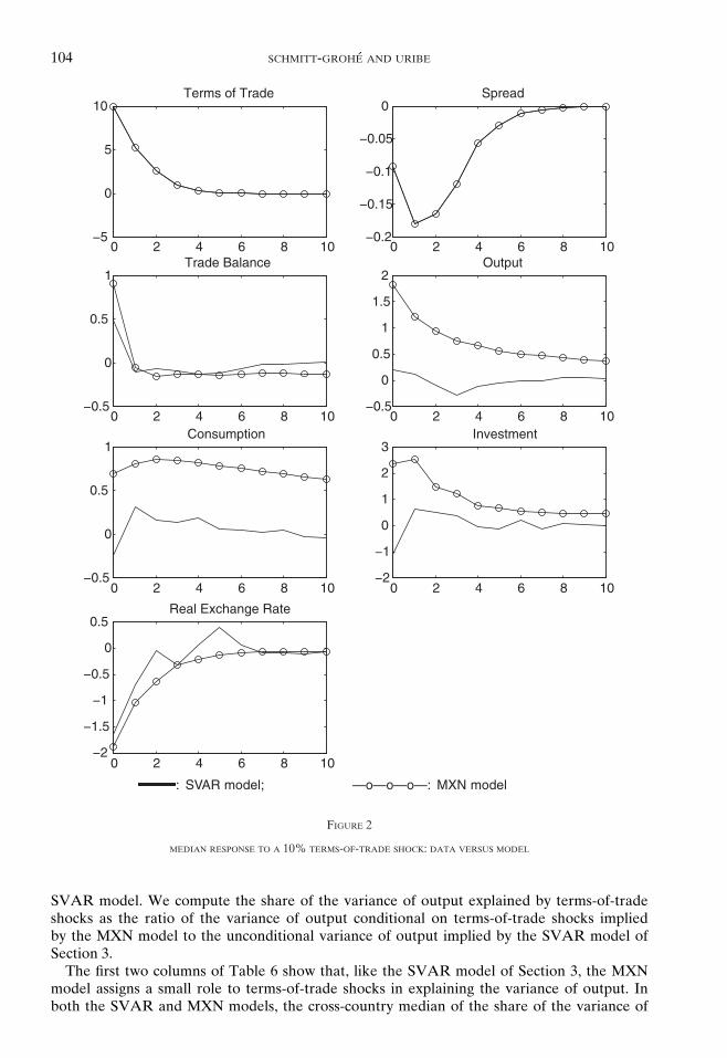
The first two columns of Table 6 might give the impression that the SVAR and MXN modelsspeak with the same voice, as both predict that on average terms-of-trade shocks explain lessthan 10% of the variance of output. This conclusion, however, would be misplaced, because thepicture that emerges from a country-by-country analysis suggests a different interpretation.

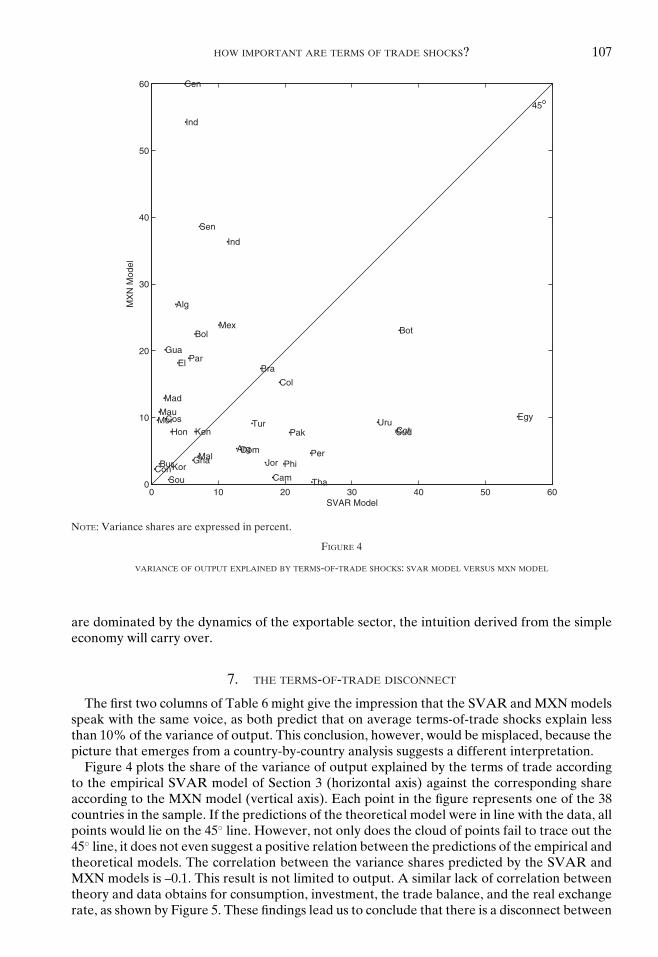
Figure 4 plots the share of the variance of output explained by the terms of trade accordingto the empirical SVAR model of Section 3 (horizontal axis) against the corresponding shareaccording to the MXN model (vertical axis). Each point in the figure represents one of the 38countries in the sample. If the predictions of the theoretical model were in line with the data, allpoints would lie on the 45◦ line. However, not only does the cloud of points fail to trace out the45◦ line, it does not even suggest a positive relation between the predictions of the empirical andtheoretical models. The correlation between the variance shares predicted by the SVAR andMXN models is –0.1. This result is not limited to output. A similar lack of correlation betweentheory and data obtains for consumption, investment, the trade balance, and the real exchangerate, as shown by Figure 5. These findings lead us to conclude that there is a disconnect between


0 20 40 600

20

40

60

45o

Consumption

SVAR Model

MX

N M

od

el

0 20 40 600

20

40

60

45o

Investment

SVAR Model

MX

N M

od

el

0 20 40 600

20

40

60

45o

Real Exchange Rate

SVAR Model

MX

N M

od

el

0 20 40 600

20

40

60

45o

Trade Balance

SVAR Model

MX

N M

od

el

NOTE. Variance shares are expressed in percent.

FIGURE 5

VARIANCE OF CONSUMPTION, INVESTMENT, THE TRADE BALANCE, AND THE REAL EXCHANGE RATE EXPLAINED BY

TERMS-OF-TRADE SHOCKS: SVAR MODEL VERSUS MXN MODEL

data and model when it comes to the importance of terms-of-trade shocks as a source of businesscycles.

8. CONCLUSION

In this article, we argue that when one looks at the data through the lens of SVAR models,terms-of-trade shocks play a modest role in generating aggregate fluctuations in emerging andpoor countries. A panel of 38 countries containing annual data from 1980 to 2011 yields amedian contribution of terms of trade to the overall variance of output of less than 10%.

This result is at odds with the standard view, built on the predictions of calibrated micro-founded dynamic business-cycle models, according to which terms-of-trade disturbances explainat least 30% of movements in aggregate activity. We formulate a more flexible specificationof this framework and estimate key structural parameters using country-level data. We findthat, when macroeconomic variables are measured in the same units in the theoretical modelas in the data on average across countries, this specification predicts that terms-of-trade shocksalso explain less than 10% of movements in aggregate activity, which is broadly in line withthe predictions of the SVAR model. However, although the importance assigned to terms-of-trade shocks by the theoretical model is on average similar to that predicted by the empiricalSVAR model, the predictions of the two models at the country level are far apart. For output,


consumption, investment, the trade balance, and the real exchange rate, there is a near-zerocross-country correlation between the share of variance attributed to terms-of-trade shocks bythe theoretical model and by the empirical model.

The resolution of the disconnect is likely to involve a combination of better empirical andtheoretical models as means to interpret the data. For example, an improvement in the empiricalmodel could stem from entertaining the hypothesis that commodity prices are a better measureof the terms of trade than aggregate indices of export and import unit values—the measure usedin the present study. At the same time, the theoretical model could be amended by assumingthat the government uses tax or commercial policy to isolate the country from swings in worldprices. In this case, movements in the terms of trade will elicit attenuated incentives to changethe domestic allocation of output and absorption. A related reason that fluctuations in the termsof trade may have different effects across countries could be the presence of different degrees ofnominal rigidities, which may introduce country-specific wedges between domestic and worldprices.

Finally, in the present study we produce country-specific estimates of several but not all of thestructural parameters of the theoretical model. Expanding the number of parameters estimatedat the country level may ameliorate the terms of trade disconnect. This task, however, isnot an easy one. The reason is that all of the parameters that we left out of the country-specific estimation affect the deterministic steady state of the model. In turn, multiple-goodsgeneral-equilibrium models, like the MXN model studied in this article, deliver steady statesthat are highly nonlinear, making their numerical solution time consuming. At the writing ofthis article, this complication renders the application of econometric techniques that rely onrepeated solutions of the steady state of the model, such as likelihood-based or GMM methods,impractical.

APPENDIX

Description of Data Sources. Unless noted otherwise the data source is the World Bank’sWDI database. The raw data from this source consists of the following annual time series.

(1) Pxt

Pmt

, Net barter terms of trade index (2000 = 100), TT.PRI.MRCH.XD.WD(2) yo

t , GDP per capita in constant local currency units, NY.GDP.PCAP.KN.

(3) Pit It

Pyt Yt

, Gross capital formation (% of GDP), NE.GDI.TOTL.ZS.

(4) Pmt Mt

Pyt Yt

, Imports of goods and services (% of GDP), NE.IMP.GNFS.ZS.

(5) Pxt Xt

Pyt Yt

, Exports of goods and services (% of GDP), NE.EXP.GNFS.ZS.

(6) Pct Ct

Pyt Yt

, Household final consumption expenditure, etc. (% of GDP), NE.CON.PETC.ZS.(7) GDP per capita, PPP (constant 2005 international $), NY.GDP.PCAP.PP.KD.(8) Consumer price index (2010 = 100), FP.CPI.TOTL.(9) Official exchange rate (LCU per US$, period average), PA.NUS.FCRF.

(10) Real effective exchange rate index (2005 = 100), PX.REX.REER.

The criteria for a country to be included in the panel is to have at least 30 consecutiveannual observations on all components of the vector xt and to belong to the group of poor andemerging countries. We define the group of poor and emerging countries as all countries in theWDI database with average PPP converted GDP per capita in U.S. dollars of 2005 over theperiod 1990–2009 below 25,000 dollars. Forty-two countries satisfy these criteria. However thefinal sample has 38 countries as we exclude four (Gambia, Swaziland, Gabon, and Panama)because of faulty terms-of-trade data. We quadratically detrend each series on the longestavailable sample for that series. The SVAR is then estimated using the longest sample for allcomponents of xt, which turns out to be 1980–2011, with three exceptions: Algeria 1980–2009,Indonesia 1981–2011, and Madagascar 1980–2009. The terms-of-trade data in WDI begin in1980 and hence dictate the beginning of the sample.


The WDI does not provide CPI data for Argentina. The Argentine CPI index was taken fromINDEC until 2006 and from IPC-7-Provincias from 2007 to 2011 due to systematic underre-porting by INDEC during this period.

The data source for the corporate bond spread in the United States is Federal ReserveEconomic Data, available online at https://fred.stlouisfed.org. We use the series BAAFFM, whichis defined as Moody’s Seasoned Baa Corporate Bond Yield minus the Federal Funds Rate.The spread is monthly and covers the period July 1954 to August 2016. We drop the years forwhich we do not have 12 monthly observations, which are 1954 and 2016, and then computethe annualized (gross) spread for the years 1955–2015 as the geometric average of the monthlyspreads before detrending it.

SUPPORTING INFORMATION

Additional Supporting Information may be found in the online version of this article at thepublisher’s website:

Online Appendix

REFERENCES

AGUIRRE, E., “Business Cycles in Emerging Markets and Implications for the Real Exchange Rate,” Ph.D.Dissertation, Columbia University, 2011.

AKINCI, O., “A Note on the Estimation of the Atemporal Elasticity of Substitution Between Tradable andNontradable Goods,” mimeo, Columbia University, 2011.

———, “Global Financial Conditions, Country Spreads and Macroeconomic Fluctuations in EmergingCountries,” Journal of International Economics 91 (2013), 358–71.

BEMS, R., “Aggregate Investment Expenditures on Tradable and Nontradable Goods,” Review of Eco-nomic Dynamics 11 (2008), 852–83.

BRODA, C., “Terms of Trade and Exchange Rate Regimes in Developing Countries,” Journal of Interna-tional Economics 63 (2004), 31–58.

CORSETTI, G., L. DEDOLA, AND S. LEDUC, “International Risk Sharing and the Transmission of ProductivityShocks,” Review of Economic Studies 75 (2008), 443–73.

FERNANDEZ, A., A. GONZALEZ, AND D. RODRIGUEZ, “Sharing a Ride on the Commodities Roller Coaster:Common Factors in Business Cycles of Emerging Economies,” mimeo, IDB, 2015.

FERNANDEZ-VILLAVERDE, J., P. GUERRON-QUINTANA, J. RUBIO-RAMIREZ, AND M. URIBE, “Risk Matters: TheReal Effects of Volatility Shocks,” American Economic Review 101 (2011), 2530–61.

GARCIA-CICCO, J., R. PANCRAZI, AND M. URIBE, “Real Business Cycles in Emerging Countries?” AmericanEconomic Review 100 (2010), 2510–31.

GUST, C., S. LEDUC, AND N. SHEETS, “The Adjustment of Global External Balances: Does Partial Exchange-Rate Pass-Through to Trade Prices Matter?” Journal of International Economics 79 (2009), 173–85.

JUSTINIANO, A., AND B. PRESTON, “Can Structural Small Open Economy Models Account for the Influenceof Foreign Disturbances?” Journal of International Economics 81 (2010), 61–74.

KOSE, M. A., “Explaining Business Cycles in Small Open Economies ‘How Much Do World PricesMatter?’” Journal of International Economics 56 (2002), 299–327.

LUBIK, T. K., AND W. L. TEO, “Do World Shocks Drive Domestic Business Cycles? Some Evidence fromStructural Estimation,” mimeo, Johns Hopkins University, 2005.

MCINTYRE, K. H., “Can Non-traded Goods Solve the ‘Comovement Problem?’” Journal of Macroeco-nomics 25 (2003), 169–96.

MENDOZA, E., “Real Business Cycles in a Small-Open Economy,” American Economic Review 81 (1991),797–818.

———, “The Terms of Trade, the Real Exchange Rate, and Economic Fluctuations,” International Eco-nomic Review 36 (1995), 101–37.

MIYAMOTO, W., AND T. L. NGUYEN, “Understanding the Cross Country Effects of U.S. Technology Shocks,”mimeo, Bank of Canada, 2014.

NA, S., “Business Cycles and Labor Income Shares in Emerging Economies,” mimeo, Columbia University,2015.

NEUMEYER, P. A., AND F. PERRI, “Business Cycles in Emerging Markets: The Role of Interest Rates,”Journal of Monetary Economics 52 (2005), 345–80.


OTTO, G., “Terms of Trade Shocks and the Balance of Trade: There Is a Harberger–Laursen–MetzlerEffect,” Journal of International Money and Finance 22 (2003), 155–84.

SCHMITT-GROHE, S., AND M. URIBE, “Closing Small Open Economy Models,” Journal of InternationalEconomics 61 (2003), 163–85.

SHOUSHA, S., “Macroeconomic Effects of Commodity Booms and Busts,” mimeo, Columbia University,2015.

URIBE, M., “Exchange Rate Based Inflation Stabilization: The Initial Real Effects of Credible Plans,”Journal of Monetary Economics 39 (1997), 197–221.

———, AND Z. V. YUE, “Country Spreads and Emerging Countries: Who Drives Whom?” Journal ofInternational Economics 69 (2006), 6–36.

WHALLEY, J., Trade Liberalization Among Major World Trading Areas (Cambridge: MIT Press, 1985).

HOW IMPORTANT ARE TERMS‐OF‐TRADE SHOCKS?mu2166/tot/paper.pdf · HOW IMPORTANT ARE TERMS-OF ......

Documents

Transcript of HOW IMPORTANT ARE TERMS‐OF‐TRADE SHOCKS?mu2166/tot/paper.pdf · HOW IMPORTANT ARE TERMS-OF ......