How good are Portfolio Insurance Strategies?

Sven Balder‡ Antje Mahayni‡‡

This version: March 31, 2009

Abstract

Portfolio insurance strategies are designed to achieve a minimum level of wealthwhile at the same time participating in upward moving markets. The most promi-nent examples of dynamic versions are option based strategies with synthetic putand constant proportion portfolio insurance strategies. It is well known that,in a Black/Scholes type model setup, these strategies can be achieved as opti-mal solution by forcing an exogenously given guarantee into the expected utilitymaximization problem of an investor with CRRA utility function. The CPPIapproach is attained by the introduction of a subsistence level, the OBPI ap-proach stems from an additional constraint on the terminal portfolio value. Webring these results together in order to explain when and why OBPI strategiesare better than CPPI strategies and vice versa. We determine the utility losseswhich are caused by introducing a terminal guarantee into the unconstrainedmaximization approach. In addition, we focus on utility losses which are due tomarket frictions such as discrete–time trading, transaction costs and borrowingconstraints.

Keywords: CPPI, OBPI, portfolio insurance, borrowing constraints, tradingrestrictions, transaction costs, utility loss.

JEL: G11, G12

‡Mercator School of Management, University of Duisburg–Essen, Lotharstr. 65, 47057 Duisburg,Germany. E-mail: sven.balder@uni-due.de

‡‡Mercator School of Management, University of Duisburg–Essen, Lotharstr. 65, 47057 Duisburg,Germany. E-mail: antje.mahayni@uni-due.de

1

1. Introduction

Portfolio strategies which are designed to limit downside risk and at the same time to

profit from rising markets are summarized in the class of portfolio insurance strategies.

Among others, Grossman and Villa (1989) and Basak (2002) define a portfolio insurance

trading strategy as a strategy which guarantees a minimum level of wealth at a specified

time horizon, but also participates in the potential gains of a reference portfolio. The

most prominent examples of dynamic versions are the constant proportion portfolio in-

surance (CPPI) strategies and option–based portfolio insurance (OBPI) strategies with

synthetic puts.1 The concept of (synthetic) option–based portfolio insurance is already

introduced in Leland and Rubinstein (1976) and Brennan and Schwartz (1976).2 The

constant proportion portfolio insurance (CPPI) is introduced in Black and Jones (1987).3

The popularity of portfolio insurance strategies can be explained by various reasons.

On the side of institutional investors there are regulatory requirements including return

guarantees as well as requisitions on the risk profile. For example, Ahn et al. (1999)

consider the problem of an institution optimally managing the market risk of a given

exposure by minimizing its Value–at–Risk using options. Amongst early papers on the

optimality of portfolio insurance are also Leland (1980) and Benninga and Blume (1985).

More recently, Doskeland and Nordahl (2008) justify the existence of guarantees from

the point of an investor through behavioral models. In particular, they use cumulative

prospect theory as an example.4

Unfortunately, the justification of guarantees is less clear assuming that the investor’s

preferences can be described using the von Neumann and Morgenstern (1944) framework

of expected utility. Dating back to Merton (1971), it is well known that in a Black/Scholes

model setup and a constant relative risk aversion (CRRA) utility function, the expected

1Principally, one can distinguish between two types of portfolio insurance strategies. A risky portfolio(or benchmark index) is combined either with a risk–free asset or with a financial derivative. In particular,the first class includes dynamic versions of OBPI, stop–loss strategies, buy and holds strategies and CPPI.The second class is mainly characterized by protective put strategies, either in a static or rolling sense.Notice that, with the exception of the buy and hold and the protective put, the above strategies are alldynamic in the sense that they afford portfolio adjustments during the investment horizon.

2For the evolution of portfolio insurance we refer to Leland and Rubinstein (1976)3For the basic procedure of the CPPI see also Merton (1971).4Basically, guarantees can be explained by a different treatment of gains and losses, i.e. losses are

weighted more heavily than gains, cf. also Kahnemann and Tversky (1979) and Tversky and Kahnemann(1992).

2

utility maximizing trading rule is a constant mix strategy, i.e. the fraction of asset expo-

sure of the current wealth is to be kept constant over the time. In this case, an investment

weight below one implies that assets are bought when the asset price decreases. This is

in sharp contrast to portfolio insurance. In order to honor a terminal guarantee, the

asset exposure is to be reduced if the price of the risky asset decreases. Technically, it is

straightforward to achieve CPPI and OBPI strategies as the optimal solution of a modified

utility maximization problem which is based on an exogenously given guarantee. CPPI

strategies are optimal for an investor who derives utility from the difference between the

terminal strategy value and a given subsistence level. In contrast, the OBPI is optimal for

an CRRA investor if one exogenously adds the restriction that the terminal portfolio value

is above the floor.5 These results are well known in the literature. Without postulating

completeness, we refer to the works of Cox and Huang (1989), Brennan and Schwartz

(1989), Grossman and Villa (1989), Black and Perold (1992), Grossman and Zhou (1993,

1996), Basak (1995), Cvitanic and Karatzas (1995, 1999), Browne (1999), Tepla (2000,

2001), Basak (2002) and El Karoui et al. (2005). Cox and Leland (2000) consider the

inverse problem. They analyze if a specific dynamic strategy can be explained by solving

the maximization problem of an expected utility maximizing investor, i.e. they analyze if

a given investment strategy is consistent with expected utility maximization. In partic-

ular, they show that a strategy which implies a path–dependent payoff is not consistent

with utility maximization in a Black/Scholes–type model.

Another strand of the literature analyzes robustness properties of stylized strategies.6

The properties of continuous–time CPPI strategies are studied extensively in the litera-

ture, cf. Bookstaber and Langsam (2000) or Black and Perold (1992). A comparison of

OBPI and CPPI (in continuous time) is given in Bertrand and Prigent (2002a). Zagst

and Kraus (2008) also compare OBPI and CPPI strategies. In particular, they derive pa-

rameter conditions implying second– and third–order stochastic dominance of the CPPI

strategy. The literature also deals with the effects of jump processes, stochastic volatility

models and extreme value approaches on the CPPI method, cf. Bertrand and Prigent

(2002b), Bertrand and Prigent (2003). An analysis of gap risk, i.e. the risk that the

guarantee is violated, is provided in Cont and Tankov (2007) and Balder et al. (2009).7

5In particular, the difference of OBPI and CPPI can be explained by the difference between postulatingthat the marginal utility jumps discontinuously to infinity or gradually, cf. for example Basak (2002).

6With respect to the robustness of option hedges we refer the reader to Avellaneda et al. (1995), Lyons(1995), Bergman et al. (1996), El Karoui et al. (1998), Hobson (1998), Dudenhausen et al. (1998) andMahayni (2003).

7Cont and Tankov (2007) introduce the gap risk by jump–diffusion models. Balder et al. (2009)introduce the gap by trading restrictions such that the analysis also captures the effects of transaction

3

Finally, there is also a a wide strand of empirical papers which measure the performance

of portfolio insurance strategies. For example, we refer to Cesari and Cremonini (2003)

who give an extensive simulation comparison of popular dynamic strategies of asset allo-

cation.

The following paper mitigates between expected utility maximization and the compari-

son of stylized strategies. We start with an exposition of the three optimization problems

which imply constant mix, CPPI and OBPI strategies as optimal. Instead of giving a

further justification for the existence of guarantees, we use the (well known) results of the

optimization problems to explain the main differences between portfolio insurance mech-

anisms. Comparing the terminal payoffs shows that both portfolio insurance strategies,

CPPI and OBPI, result in payoffs which consist of a fraction of the payoff of a constant

mix strategy (which is optimal for the unconstrained CRRA investor) and an additional

term due to the guarantee. The additional term provides an intuitive way to explain the

main advantage of the OBPI approach as compared to the CPPI approach. Intuitively, it

is clear that the fraction of wealth which is put into the optimal unconstrained stratgey

is linked to the price of the guarantee, i.e. the fraction is less than one. In the case of the

CPPI approach, the additional term is simply the guarantee itself, i.e. the payoff of an

adequate number of zero bonds. In contrast, the additional term implied by the OBPI

is a put option where the (synthetic) underlying is given by the fraction of constant mix

strategy and the strike is equal to the guarantee. Obviously, the put is cheaper than the

zero bonds. Therefore, an investor who follows the OBPI approach puts a larger fraction

of his wealth into the unconstrained optimal portfolio than an investor who follows the

CPPI approach. To asses the utility costs of forcing a guarantee into the unconstrained

problem, i.e. the utility costs from having to use a suboptimal strategy, we compare the

certainty equivalents of the different strategies and calculate the loss rates.

In addition, we explain one major drawback of the OBPI method which is due to the

kink in the payoff-profile caused by the option component. The terminal value of the

OBPI is equal to the guarantee if the put expires out of the money. In contrast to the

CPPI method, this implies a positive point mass for the event that the terminal value is

equal to the guarantee. The probability is given by the real world probability that the

terminal asset prices is below the strike of the put. Intuitively, it is clear that this can

cause a high exposure to gap risk, i.e. the risk that the guarantee is violated, if market

costs. In practice the gap risk was already observable during the 1987 crash. In addition, the crash issometimes even explained or seen to be supported by the portfolio protection mechanisms. However,there are also contradicting opinions, cf. Leland (1988). The failure of the portfolio protection gave riseto a reduction in the application of portfolio insurance strategies.

4

frictions are introduced. We illustrate this effect by taking trading restrictions and trans-

action costs into account. It turns out that the guarantee implied by the CPPI method

is relatively robust. In contrast, the probability that the guarantee is not reached under

the corresponding synthetic discrete-time OBPI strategy is rather high.

The outline of the paper is as follows. In Section 2, we review the well known optimiza-

tion problems yielding constant mix, CPPI and OBPI strategies as optimal solutions. We

compare the optimal strategies and resulting payoffs, and we discuss some advantages

(disadvantages) of the different portfolio insurance methods. In Section 3, we consider

the utility losses caused by the introduction of strictly positive terminal guarantees for a

CRRA investor. In particular, we compare CPPI and OBPI strategies according to their

implied loss rate. We consider the effects of market frictions in Section 4 where we focus

on the loss rates which are implied by discrete–time trading and transaction costs. In ad-

dition, we compare the effects of these market frictions on the protection mechanisms of

CPPI and OBPI. In Section 5, we address the topic of borrowing constrains and consider

the capped version of CPPI strategies. Section 6 concludes the paper.

2. Optimal Portfolio Selection with Finite Horizons

All stochastic processes are defined on a stochastic basis (Ω,F , (Ft)t∈[0,T ∗], P ) which sat-

isfies the usual hypotheses. We consider two assets. The riskless bond B grows at a

constant interest rate r, i.e. dBt = Btr dt where B0 = b. The evolution of the risky asset

S, a stock or benchmark index, is given by a geometric Brownian motion

dSt = St (µ dt + σ dWt) , S0 = s (1)

where W = (Wt)0≤t≤T denotes a standard Brownian motion with respect to the real world

measure P . µ and σ are constants and we assume that µ > r ≥ 0 and σ > 0.

A continuous–time investment strategy or saving plan for the interval [0, T ] can be repre-

sented by a predictable process (πt)0≤t≤T . πt denotes the proportion of the portfolio value

at time t which is invested in the risky asset S. In the following, we also refer to πt as the

portfolio weight at time t. W.l.o.g., we consider strategies which are self–financing, i.e.

money is neither injected nor withdrawn during the investment horizon [0, T ]. Thus, the

fraction of wealth which is invested at time t in the riskless bond B is given by 1 − πt.

Let V = (Vt)0≤t≤T denote the portfolio value process associated with the strategy π, then

the dynamics of V are given by

dVt(π) = Vt

(πt

dSt

St

+ (1− πt)dBt

Bt

), where V0 = x. (2)

5

For the above model assumptions, it follows

dVt(π) = Vt [(πt(µ− r) + r) dt + πtσ dWt] , where V0 = x. (3)

Alternatively, the strategies can be represented by the number of shares. Let ρt =

(ρt,S, ρt,B)0≤t≤T where ρt,S denotes the number of risky assets and ρt,B the number of

zero bonds with maturity T which are held at time t. In particular, we have

ρt,S =πtVt

St

and ρt,B =(1− πt)Vt

Bt

(4)

where Bt denotes the t–price of the zero bond maturing at T . Traditionally, a strategy

specification via the portfolio weights is used in the context of portfolio optimization

while the convention of stating the number of shares is normally preferred in the context

of hedging.

In the case of a finite investment horizon T and no intermediate consumption possibilities,

the relevant optimization problem is given by

supπ∈Π

IEP [u (VT (π))] subject to Equation (3), (5)

where Π denotes the set of all self–financing trading strategies. The utility function u

(u ∈ C2) is assumed to be strictly increaing and concave, i.e. u′ > 0 and u′′ < 0. In

the following, we recall the well known optimization problems which justify three basic

strategy classes: constant mix (CM) strategies, constant proportion portfolio insurance

strategies (CPPI) and option based strategies (OBPI). In contrast to a CM strategy which

is exclusively specified by a constant portfolio weight m, i.e. πCMt = m, portfolio insurance

strategies incorporate a guarantee component which, in the simplest case, is given by an

amount GT which is to be honored at the end of the investment horizon T . While a CPPI

strategy is value based in the sense that the portfolio weights are exclusively specified

by the current portfolio value (and the present value of the guarantee), the (dynamic)

OBPI approach is payoff and model dependent. Here, the investment decisions are, in

a complete model, given in terms of the delta hedge of an option payoff. Formally, the

three strategy classes are:

ΠCM = π ∈ Π |πt = m,m ≥ 0 (6)

ΠCPPIG =

π ∈ Π

∣∣∣∣πt = mVt − e−r(T−t)GT

Vt

,m ≥ 0

(7)

ΠOBPIG =

π ∈ Π

∣∣∣∣πt =∆tSt

Vt

, ∆t =∂

∂St

IEP ∗[e−r(T−t) (h(ST )−GT )+ |Ft

],

h ∈ C2,

(∂P ∗

∂P

)

T

= e−12(

µ−rσ )

2T−µ−r

σWT

. (8)

6

Optimization problems

problem utility function (γ > 0, γ 6= 1) additional constraint optimal strategy

(A) uA (VT ) =V 1−γ

T

1−γnone CM

(B) uB (VT ) = (VT−GT )1−γ

1−γnone CPPI

(C) uA (VT ) =V 1−γ

T

1−γVT ≥ GT OBPI

Table 1. Benchmark optimization problems.

Notice that for GT = 0, we have ΠCM = ΠCPPIG . However, we refer to CPPI and OBPI

versions where the guarantee is not a strategy parameter but GT > 0 is exogenously given.

In particular, we assume that GT < V0erT .

Table 1 summarizes the optimization problems which are suited to justify the three strat-

egy classes. Problem (A) is the classic Merton problem, cf. Merton (1971). Problem

(B) introduces a subsistence level GT such that uB belongs to the class of HARA utility

functions. Problem (C) consists of the CRRA utility function uA which is also used in

problem (A) but poses an additional constraint on the terminal value of the strategy, i.e.

the constraint that the terminal strategy value must be above or equal to the terminal

guarantee GT . The solutions of the optimization problems and their corresponding proofs

are well known in the literature such that we omit some technical parts of the proofs and

refer to the literature given in the introduction.

Intuitively, it is clear that the solutions of problems (B) and (C) are modifications of

the classic Merton problem where a guarantee is exogenously forced into the optimization

problem, respectively the solution. Basically, the subsistence level in (B) results in the

optimization problem of (A) if the value process is reduced by the present value of the

terminal guarantee, i.e. the optimization problem (A) is given in terms of the cushion

process. Technically, the solution of problem (C) is more involved. However, the solution

of (C) is intuitive in the sense that the constraint on the terminal value features an Eu-

ropean option on the optimal payoff of (A) where the initial investment must take into

account the price of the option.

2.1. Problem (A). The basic observation which simplifies the optimization problem (A)

to a large extend is the independence of the optimal portfolio weight of the investment

horizon T and the current asset price S0. This implies that the solution of problem (A)

can be obtained by restricting the strategy set to constant mix (CM) strategies such that

7

it is enough to consider the maximization problem

supπ∈ΠCM

IEP [uA (VT (π))] subject to Equation (3).

Notice that for π ∈ ΠCM , Equation (3) simplifies to

dV CMt = V CM

t [(r + m(µ− r)) dt + mσ dWt] (9)

i.e. V CMT = V CM

0 e(r+m(µ−r)− 12m2σ2)T+mσ WT . (10)

Inserting σWT = ln ST

S0− (

µ− 12σ2

)T gives8

V CMT = V CM

0 e(m(µ−r)+r− 12m2σ2)T−m(µ− 1

2σ2)T

(ST

S0

)m

= φ(V CM

0 ,m)Sm

T (11)

where φ(x, y) := x

(1

S0

)y

e(1−y)(r+ 12yσ2)T . (12)

The expected utility is equal to

IEP

[uA(V CM

T )]

=φ

(V CM

0 ,m)1−γ

1− γIE

[S

(1−γ)mT

]

=(V CM

0 )1−γ

1− γe(1−γ)(r+m(µ−r)− 1

2γm2σ2)T . (13)

Finally, it is straightforward to show that

argmaxmIEP

[uA(V CM

T )]

=µ− r

γσ2=: m∗ (14)

2.2. Problem (B). Consider now the (modified) portfolio planning problem of an in-

vestor who derives utility from the difference between the portfolio value and a given sub-

sistence level. Let C = (Ct)0≤t≤T denote the cushion process where Ct := Vt − e−rT GT .

If a constant proportion m of the cushion is invested in the risky asset, one obtains

analogously to the Equations (9) and (11)

dCt = Ct [(r + m(µ− r)) dt + mσ dWt] (15)

and CT = φ (C0,m) SmT (16)

as well as

argmaxmIEP [uA(CT )] = argmaxmIEP [uA (φ (C0,m) SmT )] =

µ− r

γσ2= m∗. (17)

8Notice that, as a function of the terminal asset price ST , the payoff V CMT is concave for m < 1, linear

for m = 1 and convex for m > 1.

8

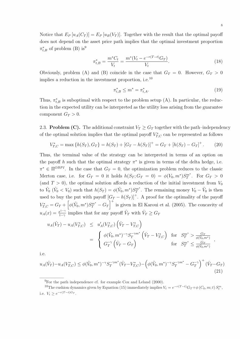
Notice that EP [uA(CT )] = EP [uB(VT )]. Together with the result that the optimal payoff

does not depend on the asset price path implies that the optimal investment proportion

π∗t,B of problem (B) is9

π∗t,B =m∗Ct

Vt

=m∗(Vt − e−r(T−t)GT )

Vt

. (18)

Obviously, problem (A) and (B) coincide in the case that GT = 0. However, GT > 0

implies a reduction in the investment proportion, i.e.10

π∗t,B ≤ m∗ = π∗t,A. (19)

Thus, π∗t,B is suboptimal with respect to the problem setup (A). In particular, the reduc-

tion in the expected utility can be interpreted as the utility loss arising from the guarantee

component GT > 0.

2.3. Problem (C). The additional constraint VT ≥ GT together with the path–independency

of the optimal solution implies that the optimal payoff V ∗T,C can be represented as follows

V ∗T,C = max h(ST ), GT = h(ST ) + [GT − h(ST )]+ = GT + [h(ST )−GT ]+ . (20)

Thus, the terminal value of the strategy can be interpreted in terms of an option on

the payoff h such that the optimal strategy π∗ is given in terms of the delta hedge, i.e.

π∗ ∈ ΠOBPI . In the case that GT = 0, the optimization problem reduces to the classic

Merton case, i.e. for GT = 0 it holds h(ST ; GT = 0) = φ(V0,m∗)Sm∗

T . For GT > 0

(and T > 0), the optimal solution affords a reduction of the initial investment from V0

to V0 (V0 < V0) such that h(ST ) = φ(V0,m∗)Sm∗

T . The remaining money V0 − V0 is then

used to buy the put with payoff [GT − h(ST )]+. A proof for the optimality of the payoff

V ∗T,C = GT +

[φ(V0,m

∗)Sm∗T −GT

]+

is given in El Karoui et al. (2005). The concavity of

uA(x) = x1−γ

1−γimplies that for any payoff VT with VT ≥ GT

uA(VT )− uA(V ∗T,C) ≤ u′A(V ∗

T,C)(VT − V ∗

T,C

)

=

φ(V0,m∗)−γS−γm∗

T

(VT − V ∗

T,C

)for Sm∗

T > GT

φ(V0,m∗)

G−γT

(VT −GT

)for Sm∗

T ≤ GT

φ(V0,m∗)

,

i.e.

uA(VT )−uA(V ∗T,C) ≤ φ(V0,m

∗)−γS−γm∗T (VT−V ∗

T,C)−(φ(V0,m

∗)−γS−γm∗T −G−γ

T

)+

(VT−GT )

(21)

9For the path independence cf. for example Cox and Leland (2000).10The cushion dynamics given by Equation (15) immediately implies Vt = e−r(T−t)GT +φ (C0, m; t)Sm

t ,i.e. Vt ≥ e−r(T−t)GT .

9

Consider the first term on the right hand side of the above inequality. Adding and

subtracting the optimal unconstrained solution V ∗T,A and taking expectations gives11

φ(V0, m∗)−γ

(IE[S−γm∗

T (VT − V ∗T,A] + IE[S−γm∗

T (V ∗T,A − V ∗

T,C)])

= 0.

Together with VT ≥ GT a.s. it follows IE[uA(VT )− uA(V ∗

T,C)]≤ 0 such that V ∗

T,C is indeed

the optimal solution w.r.t. problem (C).

The payoff V ∗T,C = GT +

[φ(V0,m

∗)Sm∗T −GT

]+

can be replicated by a self–financing

strategy where the initial investment can be represented by the expected discounted pay-

off under the uniquely defined equivalent martingale measure P ∗ defined in Equation (8),

i.e.

V0 = e−rT IEP ∗

[GT +

(φ(V0,m

∗)Sm∗T −GT

)+]

= e−rT GT + φ(V0,m∗) IEP ∗

[e−rT

(Sm∗

T − GT

φ(V0,m∗)

)+]

.

V0 has to be determined such that the initial cushion C0 = V0 − e−rT GT exactly finances

φ(V0,m∗) power call options with power p = m∗ and strike K = GT

φ(V0,m∗) , i.e.

V0 − e−rT GT = φ(V0,m

∗)

PO

(0, S0; m

∗,G

φ(V0,m∗)

)(22)

where PO (t, St; p,K) denotes the t–price a power call with power p, strike K and maturity

T , i.e.12

PO (t, St; p,K) := e−r(T−t)IEP ∗[(Sp

T −K)+ |Ft

]

= e−r(T−t)

[(St

e−r(T−t)

)pe−

12p(1−p)σ2(T−t)N

(h1

(t, St

e−r(T−t) p√K

)− (1− p)σ

√T − t

)(23)

−KN(

h2

(t, St

e−r(T−t) p√K

) )].

11Consider the portfolio VT (ε) = εV ∗T,A +(1− ε)VT . The first order condition of optimization problem

(A) implies

∂IE [u(VT (ε))]∂ε

∣∣∣∣ε=1

= IE[u′(VT (ε))(V ∗

T,A − VT )]∣∣∣

ε=1= IE

[φ(V0,m

∗)−γS−γm∗

T

(V ∗

T,A − VT

)]= 0.

12The pricing formula is well known in the literature, cf. Zhang (1998), p. 597, Equation (30.3). Theproof is easily done by using a change of measure, cf. for example Esser (2003) or Mahayni and Schlogl(2008).

10

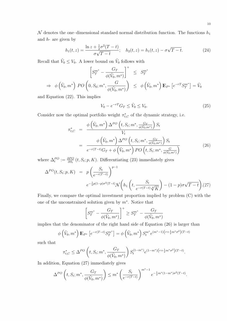
N denotes the one–dimensional standard normal distribution function. The functions h1

and h” are given by

h1(t, z) =ln z + 1

2σ2(T − t)

σ√

T − t; h2(t, z) = h1(t, z)− σ

√T − t. (24)

Recall that V0 ≤ V0. A lower bound on V0 follows with[Sm∗

T − GT

φ(V0,m∗)

]+

≤ Sm∗T

⇒ φ(V0,m

∗)

PO

(0, S0; m

∗,G

φ(V0,m∗)

)≤ φ

(V0,m

∗)

IEP ∗[e−rT Sm∗

T

]= V0

and Equation (22). This implies

V0 − e−rT GT ≤ V0 ≤ V0. (25)

Consider now the optimal portfolio weight π∗t,C of the dynamic strategy, i.e.

π∗t,C =φ

(V0,m

∗)

∆PO(t, St; m

∗, GT

φ(V0,m∗)

)St

Vt

=φ

(V0,m

∗)

∆PO(t, St; m

∗, GT

φ(V0,m∗)

)St

e−r(T−t)GT + φ(V0,m∗

)PO

(t, St; m∗, G

φ(V0,m∗)

) (26)

where ∆POt := ∂PO

∂St(t, St; p,K). Differentiating (23) immediately gives

∆PO(t, St; p,K) = p

(St

e−r(T−t)

)p−1

e−12p(1−p)σ2(T−t)N

(h1

(t,

St

e−r(T−t) p√

K

)− (1− p)σ

√T − t

).(27)

Finally, we compare the optimal investment proportion implied by problem (C) with the

one of the unconstrained solution given by m∗. Notice that[Sm∗

T − GT

φ(V0,m∗)

]+

≥ Sm∗T − GT

φ(V0,m∗)

implies that the denominator of the right hand side of Equation (26) is larger than

φ(V0,m

∗)

IEP ∗[e−r(T−t)Sm∗

T

]= φ

(V0,m

∗)

Sm∗t e(m∗−1)(r+ 1

2m∗σ2)(T−t)

such that

π∗t,C ≤ ∆PO

(t, St; m

∗,GT

φ(V0,m∗)

)S

(1−m∗)t e(1−m∗)(r+ 1

2m∗σ2)(T−t).

In addition, Equation (27) immediately gives

∆PO

(t, St; m

∗,GT

φ(V0,m∗)

)≤ m∗

(St

e−r(T−t)

)m∗−1

e−12m∗(1−m∗)σ2(T−t).

11

Basic parameter constellation

model paramter strategy parameter terminal guarantee

S0 = 1 V0 = 1 GT = 1

σ = 0.15 T = 10

r = 0.03 γ = 1.2

µ = 0.085 m = m∗ = 2.037Table 2. Basic parameter constellation.

Optimal payoffs

0.0 0.5 1.0 1.5 2.0 2.5 3.0

0

1

2

3

4

5

terminal asset price

payo

ff

Figure 1. Optimal payoffs V ∗T,A (solid line), V ∗

T,B (dotted line) and V ∗T,C

(dashed line) where the parameters are given as in Table 2.

Together, we have

π∗t,C ≤ m∗. (28)

Analogously to the problem (B), the terminal constraint in problem (C) also gives rise to

a reduction of the optimal unconstrained portfolio weight m∗.

2.4. Comparison of optimal solutions. Recall that the optimal terminal payoffs V ∗T do

not depend on the asset price path such that they can be exclusively specified in the

terminal asset price ST .13 The optimal payoffs for the optimization problems (A), (B)

13In particular, the payoffs are concave for m < 1, linear for m = 1 and convex for m > 1.

12

and (C) are summarized as follows

V ∗T,A = φ (V0,m

∗) Sm∗T (29)

V ∗T,B = GT + φ

(V0 − e−rT GT ,m∗) Sm∗

T = GT +V0 − e−rT GT

V0

V ∗T,A (30)

and V ∗T,C = GT +

[φ

(V0,m

∗)

Sm∗T −GT

]+

(31)

= φ(V0,m

∗)

Sm∗T +

[GT − φ

(V0,m

∗)

Sm∗T

]+

(32)

=V0

V0

V ∗T,A +

[GT − V0

V0

V ∗T,A

]+

. (33)

The payoff V ∗T,A corresponds to φ (V0,m

∗) power claims with power m∗ where the number

φ (V0,m∗) depends on the initial investment and the optimal investment proportion m∗.

The optimization problem (B) introduces a subsistence level which implies that the num-

ber of power claims with power m∗ must be reduced to afford the risk–free investment

which is necessary to honor the guarantee. In consequence the portfolio weight is lower

than in the case of problem (A), cf. Inequality (19). The link between the solutions of

(A) and (B) is even more explicit if one considers the number of shares in the asset which

are held. Notice that the cushion dynamics, cf. Equation (15) implies thatCCPPI

t

CCPPI0

=V CM

t

V0

if the multiplier m of the CPPI is equal to the portfolio weight of the CM strategy. In

particular, this implies that the value of the cushion is proportional to the value of the

CM strategy, i.e. CCPPIt = C0

V0V CM

t . This is also true for the number of assets ρt,S, i.e.

ρCPPIt,S =

C0

V0

ρCMt,S (34)

ρCPPIt,B = GT +

C0

V0

ρCMt,B (35)

where ρt,B denotes the number of zero bonds with maturity T . In particular, it holds that

V CPPIt = e−r(T−t)GT +

C0

V0

V CMt . (36)

The CPPI strategy can thus be interpreted as a buy and hold strategy of a constant mix

strategy with an additional investment into GT zero bonds, cf. also Equation (31). A

similar reasoning applies to the solution of (C) which can be interpreted as a buy and

hold strategy of a constant mix strategy with an additional investment into a put with

strike GT , cf. Equation (33). Obviously, the put is worth less than GT zero bonds such

that one can buy and hold more CM strategies in the case of the option based approach,

i.e. V0

V0≥ C0

V0. Intuitively, it is thus clear that the OBPI approach gives a better result

than the CPPI approach with respect to a utility function which favors the CM strategy

with portfolio weight m∗.

13

In general, a modification of the payoff V ∗T,A which honors the guarantee GT and with

t0–price equal to V0 can be represented by

GT + α

[V ∗

T,A − βGT

α

]+

subject to IEP ∗

[e−rT

(GT + α

[V ∗

T,A − βGT

α

]+)]

= V0. (37)

The CPPI approach corresponds to β = 0 and gives a smooth payoff–profile. β = 1 results

in the OBPI approach with a kinked payoff–profile. As a consequence of the guarantee

GT , both payoffs V ∗T,B and V ∗

T,C are higher (lower) than V ∗T,A for low (high) terminal asset

prices. However, the smooth solution V ∗T,B implies that the intersection with V ∗

T,A occurs

at a higher asset price ST if compared to the intersection of V ∗T,C and V ∗

T,A. Let si,j (i 6= j,

i, j ∈ A,B,C) denote the terminal asset price ST such that V ∗T,i = V ∗

T,j. Equation (30)

immediately gives

V ∗T,A = V ∗

T,B ⇔ V ∗T,A = V0e

rT

such that

sA,B = S0e(r+ 1

2(m−1)σ2)T . (38)

With Equation (33), V0 ≤ V0 and V0 ≥ e−rT GT it follows

sA,C = S0e1m

(g−r)T e(r+ 12(m−1)σ2)T = e

1m

(g−r)T sA,B where g :=1

Tln

GT

V0

≤ r. (39)

Finally, one obtains

sB,C = S0e1m

(ν−r)T e(r+ 12(m−1)σ2)T = e

1m

(ν−r)T sA,B where ν :=1

Tln

GT

V0 − C0

≥ r, (40)

i.e. sA,C ≤ sA,B ≤ sB,C . An illustration of the payoffs and the intersection points is given

in Figure 1.14

We end this section by emphasizing one important consequence for the two protection

mechanisms implied by the smooth and the kinked solutions, i.e. implied by the assump-

tions that marginal utility jumps gradually (respectively, discontinuously) to infinity. No-

tice that the smooth payoff V ∗T,B implies that there is no probability mass on the event

that the terminal value is equal to the guarantee GT , i.e. P(V ∗

T,B = GT

)= 0. In contrast,

14If not mentioned otherwise, all illustration which are given in the following are based on parameterssummarized in Table 2.

14

for the kinked payoff V ∗T,C it holds15

P(V ∗

T,C = GT

)= P

(φ

(V0,m

∗)

Sm∗T ≤ GT

)= P

ln

ST

S0

≤ ln

m∗√

GT

φ(V0,m∗)

S0

.

Using the definition of φ, cf. Equation (12), and inserting m∗ = µ−rγσ2 yields

P(V ∗

T,C = GT

)= 1−N

ln V0

e−rT GT− 1

2

(λγ

)2

T

λγ

√T

+ λ√

T

where λ :=

µ− r

σ. (41)

3. Utility loss caused by guarantees

3.1. Justification of guarantees and empirical observations. There are a few com-

ments necessary concerning the justification of guarantees. The optimization problems

(B) and (C) are already based on an exogenously postulated guarantee such that one

might doubt their capacity to give a meaningful justification of guarantees. However,

there are some arguments which are in favor of a subsistence level. Similar reasonings are

true with respect to optimization problem (C). In consequence, to some extent, guarantees

can be explained with respect to the assumption that the investor’s preferences can be

described using the von Neumann and Morgenstern (1944) framework of expected utility.

More recently, Doskeland and Nordahl (2008) justify the existence of guarantees through

behavioral models. In particular, they use cumulative prospect theory as an example.

In the following, we do not give further justifications for the existence of guarantees

or the popularity of portfolio insurance strategies but take them as given. However, we

think in terms of utility losses caused by guarantees and compare the smooth and kinked

payoff solutions. One possibility which is consistent with empirical observations is given

by measuring the utility losses of guarantees with respect to a CRRA utility function

where the parameter of risk aversion parameter is assumed to be above one (γ > 1).16

3.2. Utility loss. The performance of the strategy π can be measured by its associated

expected utility which can in turn be described by the certainty equivalent. It is defined

as certain amount which makes the investor indifferent between achieving this certain

15Intuitively it is clear that a positive point mass on the event VT = GT might indicate that thecorresponding strategy is sensitive to the introduction of gap risk which is caused by asset price jumps.This problem is considered in the Sec. 4 where trading restrictions in the sense of discrete time tradingand transaction costs are introduced.

16With respect to the literature about the validity of CRRA utility functions and the parameter ofrisk aversion we refer to Munk (2008) and the literature given herein.

15

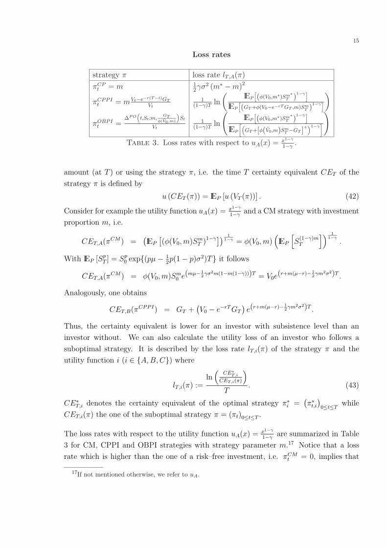
Loss rates

strategy π loss rate lT,A(π)

πCPt = m 1

2γσ2 (m∗ −m)2

πCPPIt = mVt−e−r(T−t)GT

Vt

1(1−γ)T

ln

(IEP

[(φ(V0,m∗)Sm∗

T )1−γ

]

IEP

[(GT +φ(V0−e−rT GT ,m)Sm

T )1−γ

])

πOBPIt =

∆PO(t,St;m,

GTφ(V0,m)

)St

Vt

1(1−γ)T

ln

(IEP

[(φ(V0,m∗)Sm∗

T )1−γ

]

IEP

[(GT +[φ(V0,m)Sm

T −GT ]+

)1−γ]

)

Table 3. Loss rates with respect to uA(x) = x1−γ

1−γ.

amount (at T ) or using the strategy π, i.e. the time T certainty equivalent CET of the

strategy π is defined by

u (CET (π)) = IEP [u (VT (π))] . (42)

Consider for example the utility function uA(x) = x1−γ

1−γand a CM strategy with investment

proportion m, i.e.

CET,A(πCM) =(IEP

[(φ(V0,m)Sm

T )1−γ]) 11−γ = φ(V0,m)

(IEP

[S

(1−γ)mT

]) 11−γ

.

With IEP [SpT ] = Sp

0 exp(pµ− 12p(1− p)σ2)T it follows

CET,A(πCM) = φ(V0,m)Sm0 e(mµ− 1

2γσ2m(1−m(1−γ)))T = V0e

(r+m(µ−r)− 12γm2σ2)T .

Analogously, one obtains

CET,B(πCPPI) = GT +(V0 − e−rT GT

)e(r+m(µ−r)− 1

2γm2σ2)T .

Thus, the certainty equivalent is lower for an investor with subsistence level than an

investor without. We can also calculate the utility loss of an investor who follows a

suboptimal strategy. It is described by the loss rate lT,i(π) of the strategy π and the

utility function i (i ∈ A,B, C) where

lT,i(π) :=ln

(CE∗T,i

CET,i(π)

)

T. (43)

CE∗T,i denotes the certainty equivalent of the optimal strategy π∗i =

(π∗t,i

)0≤t≤T

while

CET,i(π) the one of the suboptimal strategy π = (πt)0≤t≤T .

The loss rates with respect to the utility function uA(x) = x1−γ

1−γare summarized in Table

3 for CM, CPPI and OBPI strategies with strategy parameter m.17 Notice that a loss

rate which is higher than the one of a risk–free investment, i.e. πCMt = 0, implies that

17If not mentioned otherwise, we refer to uA.

16

Loss rates depending on m

2.04 4 60.00

0.01

0.02

0.03

0.04

0.05

0.06

m

loss

rate

2.04 4 60.00

0.01

0.02

0.03

0.04

0.05

0.06

m

loss

rate

Figure 2. Loss rates w.r.t. u = uA for CPPI (solid lines), OBPI (dashed)

and CM (dotted) strategies with varying parameter m. The parameters are

given in Table 2. The investment horizon is T = 10 years (left graph) and

T = 20 years (right graph).

the associated strategy is prohibitively bad. This critical loss rate is equal to 12γ(σm∗)2,

cf. Table 3.18 Notice that for m = m∗ it holds19

lT,A(πCP ) = 0 < lT,A(πOBPI) < lT,A(πCPPI).

For m = m∗, the utility loss implied by the guarantee is higher for the CPPI than for of

the OBPI. This is illustrated in Figure 2. In addition, notice that the loss rates of the

CM strategies are symmetric in the sense that for ε > 0, a strategy parameter m = m∗+ ε

implies the same loss rate as the parameter m = m∗ − ε. In contrast, portfolio insurance

strategies yield a lower loss rates in the case of m = m∗+ε than for m = m∗−ε. Intuitively,

this is clear since the protection feature implies that the portfolio weights of the portfolio

insurance strategies are too low compared to the optimal investment proportion m∗, cf.

Inequalities (19) and (28).

For the comparison of CPPI and OBPI, it is important to keep in mind that m∗ is the

optimal OBPI parameter for u = uA. In contrast, m∗ is not the optimal parameter for

u = uA, but for u = uB which includes a subsistence level. In order to compare the

loss rates implied by CPPI and OBPI w.r.t. u = uA, it is thus necessary to consider the

maximization problem

maxπ∈ΠCPPI

IEP [uA (VT (π))] = maxm

IEP

[(GT + φ

(V0 − e−rT GT ,m

)Sm

T

)1−γ

1− γ

]. (44)

18For the basic parameter constellation it holds 12γ(σm∗)2 = 0.056.

19For m = m∗, the inequality lT,A(πOBPI) < lT,A(πCPPI) is obvious since πCPPI is suboptimal w.r.t.the optimization problem (C) where uC = uA and πOBPI is optimal.

17

Loss rates depending on m

2.04 4 6 8 10 12 14 16 180.00

0.02

0.04

0.06

0.08

m

loss

rate

1.63 4 6 8 10 12 14 16 180.00

0.02

0.04

0.06

0.08

m

loss

rate

Figure 3. Loss rates implied by CPPI (solid lines) and OBPI (dashed

lines) for varying m, cf. Table 3. The risk aversion is γ = 1.2 (left figure)

and γ = 1.5 (right figure), for the other parameters, cf. Table 2.

Minimal loss rates

strategy γ \ T 1 2 5 10 20

CPPI 1.2 0.040 (11.32) 0.035 (7.83) 0.026 (4.91) 0.018 (3.57) 0.010 (2.73)

OBPI 1.2 0.037 (2.04) 0.031 (2.04) 0.022 (2.04) 0.014 (2.04) 0.007 (2.04)

CPPI 1.5 0.031 (10.60) 0.026 (7.25) 0.019 (4.45) 0.013 (3.16) 0.007 (2.36)

OBPI 1.5 0.028 (1.63) 0.023 (1.63) 0.015 (1.63) 0.009 (1.63) 0.005 (1.63)

CPPI 1.8 0.024 (10.03) 0.020 (6.80) 0.014 (4.10) 0.009 (2.86) 0.005 (2.08)

OBPI 1.8 0.021 (1.34) 0.017 (1.34) 0.011 (1.34) 0.007 (1.34) 0.003 (1.34)

Table 4. Minimal loss rates (uA–optimal strategy parameter m) for vary-

ing T and γ where the other parameters are given as in Table 2.

Figure 3 illustrates the loss rates for CPPI and OBPI strategies with varying parameter

m. In addition, the minimal loss rates are summarized in Table 4, i.e. the loss rates for

OBPI strategies with m = m∗ and CPPI for m = m∗∗. Although the OBPI strategy with

parameter m = m∗ is, per construction, the uA–utility maximizing portfolio insurance

strategy, the additional loss of the CPPI strategy with parameter m = m∗∗ which is mea-

sured by the difference of its loss rate and the one of the OBPI is rather low. Intuitively,

this is explained as follows...

4. Utility loss caused by trading restrictions and transaction costs

It is important to notice that in practice the concept of portfolio insurance is impeded

by market frictions. The protection mechanism of portfolio insurance implies that the

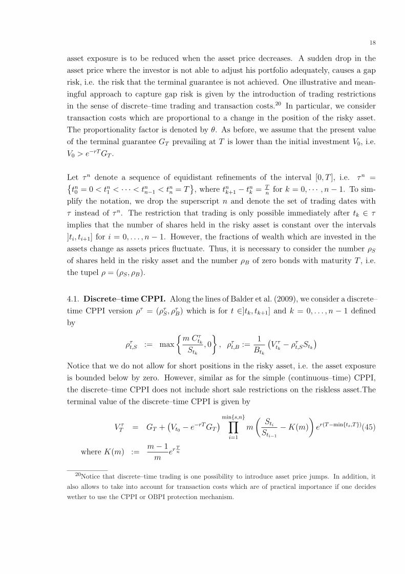
18

asset exposure is to be reduced when the asset price decreases. A sudden drop in the

asset price where the investor is not able to adjust his portfolio adequately, causes a gap

risk, i.e. the risk that the terminal guarantee is not achieved. One illustrative and mean-

ingful approach to capture gap risk is given by the introduction of trading restrictions

in the sense of discrete–time trading and transaction costs.20 In particular, we consider

transaction costs which are proportional to a change in the position of the risky asset.

The proportionality factor is denoted by θ. As before, we assume that the present value

of the terminal guarantee GT prevailing at T is lower than the initial investment V0, i.e.

V0 > e−rT GT .

Let τn denote a sequence of equidistant refinements of the interval [0, T ], i.e. τn =tn0 = 0 < tn1 < · · · < tnn−1 < tnn = T

, where tnk+1 − tnk = T

nfor k = 0, · · · , n − 1. To sim-

plify the notation, we drop the superscript n and denote the set of trading dates with

τ instead of τn. The restriction that trading is only possible immediately after tk ∈ τ

implies that the number of shares held in the risky asset is constant over the intervals

]ti, ti+1] for i = 0, . . . , n − 1. However, the fractions of wealth which are invested in the

assets change as assets prices fluctuate. Thus, it is necessary to consider the number ρS

of shares held in the risky asset and the number ρB of zero bonds with maturity T , i.e.

the tupel ρ = (ρS, ρB).

4.1. Discrete–time CPPI. Along the lines of Balder et al. (2009), we consider a discrete–

time CPPI version ρτ = (ρτS, ρτ

B) which is for t ∈]tk, tk+1] and k = 0, . . . , n − 1 defined

by

ρτt,S := max

m Cτ

tk

Stk

, 0

, ρτ

t,B :=1

Btk

(V τ

tk− ρτ

t,SStk

)

Notice that we do not allow for short positions in the risky asset, i.e. the asset exposure

is bounded below by zero. However, similar as for the simple (continuous–time) CPPI,

the discrete–time CPPI does not include short sale restrictions on the riskless asset.The

terminal value of the discrete–time CPPI is given by

V τT = GT +

(Vt0 − e−rT GT

) mins,n∏i=1

m

(Sti

Sti−1

−K(m)

)er(T−mints,T)(45)

where K(m) :=m− 1

mer T

n

20Notice that discrete–time trading is one possibility to introduce asset price jumps. In addition, italso allows to take into account for transaction costs which are of practical importance if one decideswether to use the CPPI or OBPI protection mechanism.

19

and where ts := mintk ∈ τ |Vtk < e−r(T−tk)GT and ts = ∞ if the minimum is not at-

tained. In particular, it holds that ts := mintk ∈ τ∣∣∣ Stk

Stk−1< K(m). For m > 1, the

value of the simple CPPI can drop below the floor. Therefore, the discrete–time CPPI

version introduces a gap risk, i.e. a risk that the guarantee is not honored.21

Besides discrete–time trading, we take also transaction costs into account. Along the lines

of Black and Perold (1992) we assume that the transaction costs are financed by a reduc-

tion of the asset exposure arising in the case without transaction costs, i.e.22 the discrete–

time CPPI version with transaction costs ρτ,TA =(ρτ,TA

S , ρτ,TAB

)is, for t ∈]tk, tk+1] and

k = 0, . . . , n− 1, defined by

ρτ,TAt,S := max

m Cτ,TA

tk+

Stk

, 0

, ρτ

t,B :=1

Btk

(V τ,TA

tk+− ρτ,TA

t,S Stk

).

where V τ,TAtk+

( Cτ,TAtk+

:= V τ,TAtk+

− e−r(T−tk)GT ) denotes the portfolio (cushion) value im-

mediately after tk, i.e. the value net of transaction costs which are proportional to the

asset price Stk . First, consider the portfolio value V τ,TAtk

before transaction costs, i.e.

V τ,TAt0 := Vt0 and for k = 1, . . . , n

V τ,TAtk

:= ρτ,TAtk,S Stk + ρτ,TA

tk,B Btk

= max

m Cτ,TA

tk−1+

Stk−1

, 0

Stk +

(V τ,TA

tk−1+− ρτ,TA

tk,S Stk−1

)er(tk−tk−1)

= m max

Cτ,TAtk−1+

, 0 (

Stk

Stk−1

− er(tk−tk−1)

)+ V τ,TA

tk−1+er(tk−tk−1) (46)

Consider now the adjustment to the proportional transaction costs which are due imme-

diately after the trading dates. Assuming that the transaction costs are also due at t0

and that the asset positions are transferred into a cash position immediately after tn is

21For a detailed analysis of the gap we refer to Balder et al. (2009).22This can be justified by the argument that the protection feature of the CPPI is based on a prespec-

ified riskfree investment such that the introduction of transaction costs must not change the number ofrisk free bonds which are prescribed by the CPPI method (without transaction costs).

20

consistent to the following definitions

V τ,TAt0+

:= Vt0 − ρτ,TAS,t0+

θSt0 = Vt0 −mθCτ,TAt0+

(47)

V τ,TAtk+

:= V τ,TAtk

−∣∣∣ρτ,TA

tk+,S− ρτ,TA

tk,S

∣∣∣ θStk

= V τ,TAtk

−mθ

∣∣∣∣max

Cτ,TAtk+

, 0−max

Cτ,TA

tk−1+, 0

Stk

Stk−1

∣∣∣∣ (48)

V τ,TAtn+

:= V τ,TAtn − ρτ,TA

tn,S θStn

= V τ,TAtn −mθ max

Cτ,TA

tn−1+, 0

Stn

Stn−1

. (49)

With Equation (47), it immediately follows Ct0+ := 11+θm

Ct0 . Using Equation (48) and

Equation (46) imply that for for Ctk+ > 0 (k = 0, . . . n− 1) and θ < 1m

it holds23

Ctk+1+ = Ctk+1−mθ

∣∣∣∣maxCtk+1+, 0

− Ctk+

Stk+1

Stk

∣∣∣∣ (50)

=

Ctk+

(1+θ

1+θmm

Stk+1

Stk− m−1

1+θmer T

n

)for er T

n ≤ Stk+1

Stk

Ctk+

(1−θ

1−θmm

Stk+1

Stk− m−1

1−θmer T

n

)for m−1

m(1−θ)er T

n ≤ Stk+1

Stk< er T

n

Ctk+

((1− θ)m

Stk+1

Stk− (m− 1)er T

n

)for

Stk+1

Stk< m−1

m(1−θ)er T

n

.

(51)

For Ctk+ ≤ 0 it follows Ctk+1+ = Ctk+1= er T

n Ctk+. It is worth mentioning that the

event

V τ,TAtn+

< GT

corresponds to the event that the adjusted cushion drops below

zero during the investment horizon. Notice that for, Ctk+ > 0

Ctk+1+ < 0

⇔

Stk+1

Stk

<m− 1

m(1− θ)er T

n

=: Ak+1

Since the complementary of the event∪n−1

k=0Ak+1

is given by the event that all asset

price increments are above m−1m(1−θ)

er Tn it follows with the assumption that the asset price

increments are independent and identically distributed that24

P(V τ,TA

tn+< GT

)= 1−

(P

(St1

St0

>m− 1

m(1− θ)er T

n

))n

= 1− (N (dTA

2 (θ)))n

(52)

where dTA2 (θ) :=

ln (1−θ)mm−1

+ (µ− r)Tn− 1

2σ2 T

n

σ√

Tn

(53)

23Notice that m−1m(1−θ)e

r Tn < er T

n ⇔ θ < 1m .

24In addition to the shortfall probability, the simple model setup also allows a closed–form calculationof other risk measures such as the expected shortfall, cf. Balder et al. (2009).

21

Loss rates depending on m

2 3.57 4 60.00

0.02

0.04

0.06

0.08

0.10

m

loss

rate

3 4 5 6 7

0.000

0.002

0.004

0.006

0.008

0.010

m

shor

tfal

lpro

babi

lity

Figure 4. Loss rates w.r.t. u = uA (shortfall probabilities) implied by

continuous–time CPPI (solid line), monthly CPPI without transaction costs

(dashed lines) and monthly CPPI with θ = 0.01 (dotted line) for varying

m. The parameter setup is given in Table 2.

4.2. Discrete–time option based strategy. Recall that according to Equation (26)

the (continuous–time) self–financing and duplicating strategy for the T–payoff GT +

φ(V0,m)[Sm

T − GT

φ(V0,m)

]+

is given by

ρt,S := φ(V0,m)∆PO

(t, St; m,

GT

φ(V0,m)

)(54)

ρt,B := GT +φ(V0,m)PO

(t, St; m, GT

φ(V0,m)

)− ρt,SSt

B(t, T )(55)

where ∆PO is defined as in Equation (27). We consider as a discrete–time version of

an arbitrary continuous–time trading strategy ρτ = (ρτS, ρτ

B) with respect to the trading

dates τ

ρτt := ρtnk

for t ∈]tk, tk+1] and for all t ∈ [0, T ].

Setting V0(ρ; τ) := V0(ρ), the value process V (ρ; τ) which is associated with ρτ is

Vt(ρ; τ) = ρtk,SSt + ρtk,Be−r(T−t) for t ∈]tk, tk+1] and 0 ≤ k ≤ n− 1.

Notice that, in general, the discrete–time version of a continuous–time strategy is not

self–financing. In particular, there are in– or out–flows from the portfolio which occur im-

mediately after a trading date tk+1 (k = 0, . . . , n−1). Formally, the costs of discretization

ξdistk+1

(ρ; τ) which occur immediately after the trading date tk+1 are defined by

ξdistk+1

(ρ; τ) := Vtk+1(ρ)− Vtk+1

(ρ; τ) (56)

=(ρtk+1,S − ρtk,S

)Stk+1

+(ρtk+1,B − ρtk,B

)e−r(T−tk+1). (57)

22

Loss rates depending on m

2.04 4 60.00

0.02

0.04

0.06

0.08

0.10

m

loss

rate

2.04 4 6

0.0

0.2

0.4

0.6

0.8

m

shor

tfal

lpro

babi

lity

Figure 5. Loss rates w.r.t. u = uA (shortfall probabilities) in the Merton

setup implied by continuous–time OBPI (solid line), monthly OBPI without

transaction costs (dashed lines) and monthly OBPI with θ = 0.01 (dotted

line) for varying m. The parameter setup is given in Table 2.

Notice that negative costs refer to inflows while positive costs imply that further money

is needed to continue the strategy.

Taking into account for proportional transaction costs also implies that there are trans-

action costs ξTAtk+1

(ρ; τ) which occur immediately after a trading date tk+1, i.e.

ξTAt0

(ρ; τ) := |ρt0,S|θSt0

ξTAtk+1

(ρ; τ) = |ρtk+1,S − ρtk,S|θStk+1for k = 0, . . . , n− 2

and ξTAtn (ρ; τ) := |ρtn−1,S|θStn .

Defining the payoff VT (ρ; τ) according to the assumption that the inflows into the strategy

are lent according to the interest rate r and outflows are saved according to r gives

VT (ρ; τ) := Vtn(ρ)−[ξTAt0

er(T−t0) +n−1∑

k=0

(ξdistk+1

(ρ; τ) + ξTAtk+1

(ρ; τ))

er(tn−tk+1)

]. (58)

4.3. Comments on utility loss and shortfall probability. The loss rates w.r.t.

u = uA (shortfall probabilities) of the above discrete–time versions are illustrated in

Figure 4 and Figure 5.25 Observe, that for both strategies, OBPI and CPPI, the loss

which is in the first instance caused by time–discretizing the strategies is rather low.

However, there is a huge impact caused by transaction costs where the effect is even more

25Notice that the introduction of gap risk. i.e. a strictly positive shortfall probability, gives a loss ofminus infinity in the case of u = uB and u = uC .

23

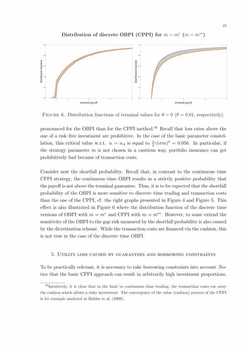
Distribution of discrete OBPI (CPPI) for m = m∗ (m = m∗∗)

1 2 4 6 80.0

0.2

0.4

0.6

0.8

1.0

terminal payoff

dist

ribu

tion

func

tion

1 2 4 6 80.0

0.2

0.4

0.6

0.8

1.0

terminal payoff

dist

ribu

tion

func

tion

Figure 6. Distribution functions of terminal values for θ = 0 (θ = 0.01, respectively).

pronounced for the OBPI than for the CPPI method.26 Recall that loss rates above the

one of a risk–free investment are prohibitive. In the case of the basic parameter constel-

lation, this critical value w.r.t. u = uA is equal to 12γ(σm)2 = 0.056. In particular, if

the strategy parameter m is not chosen in a cautious way, portfolio insurance can get

prohibitively bad because of transaction costs.

Consider now the shortfall probability. Recall that, in contrast to the continuous–time

CPPI strategy, the continuous–time OBPI results in a strictly positive probability that

the payoff is not above the terminal guarantee. Thus, it is to be expected that the shortfall

probability of the OBPI is more sensitive to discrete–time trading and transaction costs

than the one of the CPPI, cf. the right graphs presented in Figure 4 and Figure 5. This

effect is also illustrated in Figure 6 where the distribution function of the discrete–time

versions of OBPI with m = m∗ and CPPI with m = m∗∗. However, to some extend the

sensitivity of the OBPI to the gap risk measured by the shortfall probability is also caused

by the dicretization scheme. While the transaction costs are financed via the cushion, this

is not true in the case of the discrete–time OBPI.

5. Utility loss caused by guarantees and borrowing constraints

To be practically relevant, it is necessary to take borrowing constraints into account .No-

tice that the basic CPPI approach can result in arbitrarily high investment proportions.

26Intuitively, it is clear that in the limit to continuous–time trading, the transaction costs eat awaythe cushion which allows a risky investment. The convergence of the value (cushion) process of the CPPIis for example analyzed in Balder et al. (2009).

24

Incorporating borrowing constraints into the classic CPPI strategy straightforwardly re-

sults in the capped CPPI which we abbreviate with CCP.27 The capped CPPI strategy

ρCCP =(ρCCP

S , ρCCPB

)is defined by

ρCCPt,S =

min(ωV CCP

t ,mCCCPt

)

St

, ρCCPt,B =

V CCPt − ρCCP

t,S St

Bt

(59)

where CCCPt := V CCP

t − e−r(T−t)GT .

and where w (w ≥ 1) denotes the restriction on the investment proportion. In the fol-

lowing, we refer to borrowing constraints in the strict sense, i.e. we assume that ω is set

equal to one.

It is worth mentioning that the borrowing constraints introduce a path–dependence and

the payoff implied by the capped CPPI version can not be stated as a function of the

terminal asset price as it is the case without borrowing constraints. Intuitively, it is to

be expected that the path dependence yields an additional utility loss in a Black/Scholes

type model setup. In order to calculate the loss rate, we consider the distribution of the

terminal value of the CP strategy. Let f denote the density function of the terminal value

of the capped CPPI. Then it holds

IE[uA(πCCP )

]=

∫ ∞

GT

uA(v)f(v) dv

CET,A(πCCP ) =

(∫ ∞

GT

v1−γf(v) dv

) 11−γ

such that lT,A(πCCP ) =1

Tln

V0e

(r+m+(µ−r)− 12γ(m∗σ)2)T

(∫∞GT

v1−γf(v) dv) 1

1−γ

.

For details on the distribution of the capped CPPI we refer to Balder and Mahayni (2008).

Basically, the distribution can be obtained by considering the process (X)0≤t≤T which is

given by the dynamics

dXt = Θ(Xt)dt + dWt

where

Θ(x) =

µ−rσ− 1

2mσ x ≤ 0

µ−rσ− 1

2σ x > 0

and X0 =

1σ

ln (m−1)V0

mG0mC0 ≥ V0

1mσ

ln (m−1)C0

G0mC0 < V0

.

27This is also true in the case of the OBPI strategy which is based on synthesizing a power optionwith a power p > 1. However, it is not straightforward how to incorporate borrowing constraints for theOBPI. One possibility is given by setting m = 1, i.e. referring to a standard option instead of a poweroption. This is also done in practice but not considered in the following.

25

Loss rates depending on m

2.04 4 6 8 10 120.00

0.02

0.04

0.06

0.08

m

loss

rate

2.04 4 6 8 10 120.00

0.02

0.04

0.06

0.08

m

loss

rate

Figure 7. Loss rates w.r.t. u = uA implied by CPPI (solid lines) and

capped CPPI (dashed lines) for varying m. The risk aversion is γ = 1.2

(left figure) and γ = 1.5 (right figure), the other parameters are as in Table

2. The constant line gives the loss rate of a stop–loss strategy.

Along the lines of Balder and Mahayni (2008), one can show that the value process(V CCP

t

)0≤t≤T

and cushion process(CCCP

t

)0≤t≤T

are, for ω = 1, given by

V CCPt = Gt

m

m−1eσXt Xt ≥ 0(

1 + 1m−1

eσmXt)

Xt < 0(60)

and

CCCPt = Gt

(m

m−1eσXt − 1

)Xt ≥ 0

1m−1

emσXt Xt < 0.

In particular, it holds

P[V CCP

t ∈ dv]

=

1σv

p

(ln

(m−1)vmGt

σ

)dv v ≥ m

m−1Gt

1σm(v−Gt)

p

(ln

(m−1)(v−Gt)Gt

σm

)dv v < m

m−1Gt

where p(x) := PX0(Xt ∈ dx).

The loss rate implied by the capped CPPI is illustrated in Figure 7. Notice that for

m → ∞, the capped CPPI converges to the stop-loss strategy, cf. Black and Perold

(1992). Obviously, the loss rate converges, too. It is interesting to observe that the

loss-rate of the capped CPPI is smaller than the loss-rate of the stop-loss-strategy for

m ≥ m∗∗.

26

6. Conclusion

The popularity of portfolio insurance strategies including a strictly positive guarantee

component with respect to a fixed investment horizon can be explained by various reasons

like regulatory requirements or behavioral finance models. To some extend, the justifica-

tion of positive guarantees is also possible assuming that the investor’s preferences can be

described using the von Neumann Morgenstern framework of expected utility.

Dating back to Merton, it is well known that in a Black/Scholes model setup and for

a CRRA utility function, the optimal strategy is to invest a constant fraction of wealth

into the risky asset. Such a constant mix strategy implies that, for an investment pro-

portion m > 1 (m < 1), additional asset are bought (sold) if the asset price increases. In

particular, for m > 1 the resulting payoff is convex in the asset price so that a constant mix

strategy can, at least technically, be classified as a portfolio insurance strategy. However,

the payoff is floored by zero. In theory, it is straightforward to achieve optimal strategies

yielding payoffs with a positive floor. Here, the expected utility is maximized under the

additional constraint that the terminal portfolio value must be above a strictly positive

terminal guarantee. Alternatively, the floor can be achieved if the utility is measured in

terms of the difference of the portfolio value and the guarantee instead of the portfolio

wealth itself, i.e. if a utility function with a subsistence level is used.

The modified optimization problems help to understand the most prominent approaches

of portfolio insurance strategies, i.e. CPPI and OBPI strategies. The modifications which

are imposed on the unconstraint optimization problem give interesting modifications for

the payoffs. Using the unrestricted optimization problem as benchmark, the constant mix

strategy and its associated payoff with floor zero defines also a benchmark for OBPI and

CPPI strategies. The CPPI results from a subsistence level, i.e. the utility is measured in

terms of the difference of portfolio value and guarantee instead of the portfolio value itself.

In contrast, the OBPI results from the additional constraint that the terminal payoff is

above the guarantee or floor. Considering the associated payoffs, both approaches result

in payoffs which consist of a fraction of the payoff of a constant mix strategy and an

additional term stemming from the guarantee. Intuitively, it is clear that the fraction is

linked to the price of the guarantee, i.e. the fraction is less than one. The main difference

between OBPI and CPPI can easily be explained by the additional term. In the case

of the CPPI approach, the additional term is simply the guarantee itself, i.e. the payoff

of the adequate number of zero bonds. In contrast, the additional term implied by the

OBPI is based on a put on the fraction of constant mix payoffs with strike equal to the

guarantee. Obviously, the put on the zero coupon bond is cheaper than the zero bond

27

itself. Thus, the OBPI fraction which is held of the optimal unrestricted payoff is higher

than in the case of the CPPI method. This is a major advantage in terms of the associ-

ated utility costs, i.e. the loss in expected utility which is caused by the introduction of

a strictly positive guarantee. The utility costs are measured and illustrated in terms of

a loss rate linking the certainty equivalents of the strict portfolio insurance strategies to

the certainty equivalent of the optimal solution.

One major drawback of the OBPI method is due to its kinked payoff-profile. The termi-

nal value of the OBPI is equal to the guarantee if the put expires out of the money. In

contrast to the CPPI method, this implies a positive point mass that the terminal value

is equal to the guarantee. This relevant probability is given by the real world probabil-

ity that the terminal asset prices is below the strike of the put. Intuitively, it is clear

that this can cause a high exposure to gap risk, i.e. the risk that the guarantee is not

honored, if market frictions are introduced. We illustrate this effect by taking trading

restrictions and transaction costs into account. It turns out that the guarantee implied

by the CPPI method is relatively robust. However, the probability that the guarantee is

not reached under the corresponding synthetic discrete-time OBPI strategy is rather high.

Finally, we tackle the question of borrowing constraints. In a strict sense, borrowing

constraints imply that the proportion of asset must not be above one. In the case of the

CPPI method, the capped CPPI which simply states that the asset proportion is ade-

quately capped according to the borrowing constraints is of high practical relevance. We

give the distribution of the capped CPPI and illustrate the corresponding loss rate, i.e.

the loss which is due to borrowing constraints.

28

References

Ahn, D.-H., Boudoukh, Richardson, M. and Whitelaw, R. (1999), Optimal Risk

Management Using Options, Journal of Finance LIV(1), 359–375.

Avellaneda, M., Levy, A. and Paras, A. (1995), Pricing and Hedging Derivative Secu-

rities in Markets with Uncertain Volatilities, Applied Mathematical Finance 2(2), 73–88.

Balder, S. and Mahayni, A. (2008), Cash–Lock Comparison of Portfolio Insurance

Strategies, Technical reprot.

Balder, S., Brandl, M. and Mahayni, A. (2009), Effectiveness of CPPI Strategies und

Discrete–Time Trading, The Journal of Economic Dynamics and Control 33, 204–220.

Basak, S. (1995), A General Equilibrium Model of Portfolio Insurance, Review of Fi-

nancial Studies 8(4), 1059–1090.

Basak, S. (2002), A Comparative Study of Portfolio Insurance, The Journal of Economic

Dynamics and Control 26(7-8), 1217–1241.

Benninga, S. and Blume, M. (1985), On the Optimality of Portfolio Insurance, Journal

of Finance 40(5), 1341–1352.

Bergman, Y., Grundy, B. and Wiener, Z. (1996), General Properties of Option

Prices, Journal of Finance 51, 1573–1610.

Bertrand, P. and Prigent, J.-L. (2002a), Portfolio Insurance Strategies: OBPI versus

CPPI, Technical report, GREQAM and Universite Montpellier1.

Bertrand, P. and Prigent, J.-L. (2002b), Portfolio Insurance: The Extreme Value

Approach to the CPPI, Finance.

Bertrand, P. and Prigent, J.-L. (2003), Portfolio Insurance Strategies: A Comparison

of Standard Methods When the Volatility of the Stoch is Stochastic, International

Journal of Business 8(4), 15–31.

Black, F. and Jones, R. (1987), Simplifying Portfolio Insurance, The Journal of Port-

folio Management 14, 48–51.

Black, F. and Perold, A. (1992), Theory of Constant Proportion Portfolio Insurance,

The Journal of Economic Dynamics and Control 16(3-4), 403–426.

Bookstaber, R. and Langsam, J. (2000), Portfolio Insurance Trading Rules, The

Journal of Futures Markets 8, 15–31.

Brennan, M. and Schwartz, E. (1976), The Pricing of Equity–Linked Life Insurance

Policies with an Asset Value Guarantee, Journal of Financial Economics 3, 195–213.

Brennan, M. and Schwartz, E. (1989), Portfolio Insurance and Financial Market

Equilibrium, Journal of Business 62, 455–472.

Browne, S. (1999), Beating a Moving Target: Optimal Portfolio Strategies for Outper-

forming a Stochastic Benchmark, Finance and Stochastics 3, 275–294.

Cesari, R. and Cremonini, D. (2003), Benchmarking, portfolio insurance and technical

29

analysis: a Monte Carlo comparison of dynamic strategies of asset allocation, Journal

of Economic Dynamics and Control 27, 987–1011.

Cont, R. and Tankov, P. (2007), Constant Proportion Portfolio Insurance in Presence

of Jumps in Asset Prices, Financial Engigeering No 2007–10, Columbia University

Center for Financial Engigeering.

Cox, C. and Leland, H. (2000), On dynamic investment strategies, The Journal of

Economic Dynamics and Control 24, 1859–1880.

Cox, J. and Huang, C.-F. (1989), Optimal Consumption and Portfolio Policies when

the Asset Price follows a Diffusion Process, Journal of Economic Theory 49, 33–83.

Doskeland, T. M. and Nordahl, H. A. (2008), Optimal pension insurance design,

Journal of Banking and Finance 32, 382–392.

Dudenhausen, A., Schlogl, E. and Schlogl, L. (1998), Robustness of Gaussian

Hedges under Parameter and Model Misspecification, Technical report, University of

Bonn, Department of Statistics.

El Karoui, N., Jeanblanc, M. and Lacoste, V. (2005), Optimal Portfolio Manage-

ment with American Capital Guarantee, Journal of Economic Dynamics and Control

29, 449–468.

El Karoui, N., Jeanblanc-Picque, M. and Shreve, S. (1998), Robustness of the

Black and Scholes Formula, Mathematical Finance 8(2), 93–126.

Esser, A. (2003), General Valuation Principles for Arbitrary Payoffs and Applications

to Power Options under Stochastic Volatility Models, Financial Markets and Portfolio

Management 17, 351–372.

Grossman, S. and Villa, J. (1989), Portfolio Insurance in Complete Markets: A Note,

Journal of Business 62, 473–476.

Grossman, S. and Zhou, J. (1993), Optimal Investment Strategies for Controlling

Drawdowns, Mathematical Finance 3, 241–276.

Grossman, S. and Zhou, J. (1996), Equilibrium Analysis of Portfolio Insurance, Jour-

nal of Finance 51, 1379–1403.

Hobson, D. (1998), Volatility Misspecification, Option Pricing and Superreplication via

Coupling, Annals of Applied Probability 8(1), 193–205.

Kahnemann, D. and Tversky, A. (1979), Prospect Theory: An Analysis of Decision

under Risk, Econometrica 47, 263–291.

Leland, H. (1980), Who should buy Portfolio Insurance, Journal of Finance 35(2), 581–

594.

Leland, H. (1988), Portfolio Insurance and October 19th, California Management Review

Summer, 80–89.

Leland, H. and Rubinstein, M. (1976), The Evolution of Potfolio Insurance, in: D.L.

30

Luskin, ed., Portfolio Insurance: A guide to Dynamic Hedging, Wiley.

Lyons, T. (1995), Uncertain Volatility and the Risk-free Synthesis of Derivatives, Applied

Mathematical Finance 2, 117–133.

Mahayni, A. (2003), Effectiveness of Hedging Strategies under Model Misspecification

and Trading Restrictions, International Journal of Theoretical and Applied Finance

6(5), 521–552.

Mahayni, A. and Schlogl, E. (2008), The Risk Management of Minimum Return

Guarantees, Business Research 1, 55–76.

Merton, R. (1971), Optimal Consumption and Portfolio Rules in a Continuous Time

Model, Journal of Economic Theory 3, 373–413.

Munk, C. (2008), Financial asset pricing theory, Lecture notes.

Tepla, L. (2000), Optimal portfolio policies with borrowing and shortsale constraints,

The Journal of Economic Dynamics and Control 24, 1623–1639.

Tepla, L. (2001), Optimal Investment with Minimum Performance Constraints, The

Journal of Economic Dynamics and Control 25(10), 1629–1645.

Tversky, A. and Kahnemann, D. (1992), Advances in Prospect Theory: Cumulative

Representation of Uncertainty, Journal of Risk and Uncertainty 5, 297–323.

von Neumann, J. and Morgenstern, O. (1944), Theory of Games and Economic

Behavior, 1953 ed.. Princeton University Press, Princeton, NJ.

Zagst, R. and Kraus, J. (2008), Stochastic Dominance of Portfolio Insurance Strategies

– OBPI versus CPPI, Technical reprot.

Zhang, P. G. (1998), Exotic Options–A Guide to Second Generation Options, World

Scientific.