How English domiciled graduate earnings vary with gender, institution attended, subject and socio-economic background

IFS Working Paper W16/06

Jack Britton Lorraine Dearden Neil Shephard Anna Vignoles

How English domiciled graduate earnings vary with gender,

institution attended, subject and socioeconomic background∗

Jack BrittonInstitute for Fiscal Studies, London

jack b@ifs.org.uk

Lorraine DeardenInstitute for Fiscal Studies, London and Institute of Education, University College London

lorraine d@ifs.org.uk

Neil ShephardDepartment for Economics and Department of Statistics, Harvard University

shephard@fas.harvard.edu

Anna VignolesDepartment of Education, University of Cambridge

av404@cam.ac.uk

April 13, 2016

Abstract

This paper uses tax and student loan administrative data to measure how the earnings of En-glish graduates around 10 years into the labour market vary with gender, institution attended,subject and socioeconomic background. The English system is competitive to enter, with someuniversities demanding very high entrance grades. Students specialise early, nominating theirsubject before they enter higher education (HE). We find subjects like Medicine, Economics,Law, Maths and Business deliver substantial premiums over typical graduates, while disappoint-ingly, Creative Arts delivers earnings which are roughly typical of non-graduates. Considerablevariation in earnings is observed across different institutions. Much of this is explained by stu-dent background and subject mix. Based on a simple measure of parental income, we see thatstudents from higher income families have median earnings which are around 25% more thanthose from lower income families. Once we control for institution attended and subject chosen,this premium falls to around 10%.

∗Many civil servants and policy makers have helped us gain access to the data which is the core of this paper.Although it is difficult to pick out a small group who helped most, we must thank in particular Daniele Bega, DaveCartwright, Nick Hillman, Tim Leunig and David Willetts who were all crucial in making this project happen. Ofcourse we solely are responsible for any errors. We are particularly grateful to the Nuffield Foundation for theirfinancial support. The Nuffield Foundation is an endowed charitable trust that aims to improve social well-being inthe widest sense. It funds research and innovation in education and social policy and also works to build capacityin education, science and social science research. The Nuffield Foundation has funded this project, but the viewsexpressed are those of the authors and not necessarily those of the Foundation. HM Revenue & Customs (HMRC)and Student Loans Company (SLC) have agreed that the figures and descriptions of results in the attached documentmay be published. This does not imply HMRC’s or SLC’s acceptance of the validity of the methods used to obtainthese figures, or of any analysis of the results. Copyright of the statistical results may not be assigned. This workcontains statistical data from HMRC which is Crown Copyright and statistical data from SLC which is protected byCopyright, the ownership of which is retained by SLC. The research datasets used may not exactly reproduce HMRCor SLC aggregates. The use of HMRC or SLC statistical data in this work does not imply the endorsement of eitherHMRC or SLC in relation to the interpretation or analysis of the information.

1

Keywords: Administrative data; Graduate earnings; Human capital; Labour earnings; Degree

subject; Student loans.

1 Introduction

This paper uses high quality administrative tax data to provide estimates of English graduates’

earnings and shows how they vary according to gender, subject studied, institution attended and

socioeconomic background of the student. Over and above improving our understanding of the

sources of variation in graduates’ earnings, this paper can also inform issues relating to social

mobility. In England it is well known that access to university, on average, varies substantially

by the level of parental income and that students from poorer families access different types of

universities than those from wealthier backgrounds. However, the question of whether graduates’

earnings vary according to their socioeconomic background amongst graduates attending similar

universities and taking the same subject has remained poorly understood, thus far limited by data

availability. Our unique administrative database offers substantial advantages in addressing this

crucial question. The findings are also relevant for myriad other issues that benefit from better

information on variation in graduates’ earnings, including: student choice of subject and institution;

better information for schools to help advise and guide students whilst at school; and the operation

and cost of the higher education finance system.

1.1 The core of our paper

This paper is the first to use administrative tax records to provide estimates of sub-populations of

English domiciled graduates’ labour earnings over their early life course. This new and abundant

longitudinal data source allows us to study how graduates’ earnings develop and vary according

to the subject they studied, the institution they attended, their gender and an indicator of their

family’s income status. We record means and quantiles of these sub-populations. We also have

data from the UK’s Higher Education Statistics Agency (HESA) on the socioeconomic background

and pre-HE academic achievement of the students studying the same subject in the same institution

(these data are not linked to our earnings data at individual level). With these data we can estimate

a model that controls for student intake and hence enables us to report a value added measure of

the degree.

The core of our paper bores into a unique database developed and documented by Britton

et al. (2015) which was built through the hard linking of anonymised individual level data from the

English student loan book, a book owned by the UK’s Secretary of State for Business, Innovation

and Skills and operated by the Student Loan Company (SLC), with the corresponding income

2

tax records held by Her Majesty’s Revenue and Customs (HMRC), the UK tax authority. The

book starts with new borrowers from 1998 and we look in detail at tax records for the tax years

2008/09 to 2012/13. Throughout, we refer to these borrowers as graduates, though in practice we

do not observe whether they complete their course. We have several cohorts of students, from 1998

through to 2011 (though information on the latter cohorts is limited as many are still enrolled on

their courses during the years we observe), and primarily focus on the 1999-2005 cohorts. This

allows us to follow graduates through their most crucial career developing years. Hence another

contribution of this paper is to provide some insight into graduates’ earnings growth some years

into graduates’ careers, rather than just on entry into the labour market as is the case for much of

the UK literature.

Britton et al. (2015) defined the population of English domiciled student loan borrowers and

constructed the labour earnings variables for this database, as well as providing English wide

summary statistics of earnings (e.g. median earnings in the tax year 2011/12 of English former

borrowers who started HE in 1999 and are female).

For the first time we use these administrative data to characterise the properties of earnings

for sub-populations of borrowers (graduates) and shows how they vary by gender, degree subject

and higher education institution. An example of this is that we can observe the 2011/12 earnings

of female Law students at Manchester University who started at that university in 2001 (we call

this the 2001 cohort). We think about these sub-populations in a number of ways, by looking at

means and quantiles of:

• Unconditional earnings.

• Predicted earnings for this sub-population using an individual level parental income indicator

and HESA profiles of the socioeconomic background and pre-HE academic achievement of

the students in each subject/institution combination.

This second approach can be used to provide a conditional estimate of the earnings of graduates

from different institutions or taking different degree subjects, after controlling for differences in some

key characteristics of the individual or the institution and is our approximation of a value-added

measure of the university by subject. We are mindful however, that selection into degree courses

will mean that our estimates are not going to tell us about the causal impact of a particular degree

on earnings. Further we do not have detailed information about the education achievement or other

characteristics beyond gender and age of non-graduates and hence, whilst we can compare graduate

earnings to non-graduate earnings, we cannot calculate a formal rate of return on a particular

degree. Instead we focus on measures of variation in graduates’ earnings that are themselves of

3

considerable value.

The data we use and the analysis it generates is highly original. Whilst other UK surveys

such as the Labour Force Survey (LFS) and the Destinations of Leavers from Higher Education

(DLHE) survey have information on subject of study and institution, the latter has only recently

been collected by the LFS, limiting the sample sizes available to researchers. A current source of

UK data on graduate earnings by subject and institution is the DLHE survey, which looks at full

time equivalent earnings 3 years past graduation. However, our administrative data offers major

advantages in terms of scale, quality and duration. We will see that it is important to model

both institution and subject. Further, Britton et al. (2015) suggested that much of the interesting

HE impacts on earnings emerge after the 3 year horizon when postgraduate education and initial

career training has largely been completed. Certainly, the diversity of graduate earnings takes a

while to emerge, but they are on stark display after ten years when the earnings of some graduate

sub-populations are rapidly accelerating. For this reason, it is essential we observe a longer time

span of gradates’ earnings than is provided in the DLHE and our administrative data offers an

opportunity to do so.

In the rest of this section we will explain why our work matters and place our contribution in

the context of the existing literature. We also provide an outline for the rest of the paper.

1.2 Public policy

Policy change has been rapid in the English higher education system in recent years, with major

reforms to the finance system, a lifting of the cap on student numbers and some quite dramatic

changes in the composition of the student body with a large increase in the number of EU students

accessing UK higher education Dorling (2016). Against this backdrop of rapid change there is a need

to improve our understanding of the diversity of the sector and the variability in graduates’ earning

outcomes. Of course students go to university for many reasons other than for pecuniary gain

and many graduates do socially valuable jobs that are not necessarily higher paying. Nonetheless,

reliable information on graduates’ earnings is crucially important from a public policy perspective.

There are three principal reasons for us to better understand the diversity of graduates’ earnings

(given in alphabetical order rather than order of importance): (i) Funding; (ii) Information; (iii)

Social mobility.

The UK Government runs an income contingent loan system for funding English domiciled

students at UK higher education providers (HEPs). As a result, the cost to the Government

depends crucially upon the path of earnings of graduates over the first 30 years of their career (e.g.

Browne (2010), Barr (2007), Barr and Shephard (2010)). Our data enable us to measure earnings

after the first decade of a graduates’ career providing additional insights into this issue.

4

Students from all socioeconomic backgrounds need to be informed about their options. One

aspect of this, which the UK Government tries to provide using the six month and 3 year DHLE

data, is earnings data (see the unistats.direct.gov.uk website which provides the Key Information

Set (KIS) as a summary of crucial information for students for each degree course). Unfortunately,

the DHLE data misses most of the acceleration in graduate earnings which some, but by no means

all, graduate careers see (acceleration depends upon institution and subject choice). Hence the

current information available to students strongly under reports the diversity of graduate earnings

across subject and institutional choices. This is likely to be more damaging for students who come

from families and communities who are less informed about potential HE choices. This paper will

consider whether the administrative data analysed here can start to bridge this information gap.

A central focus for this paper is what the diversity of graduates’ earnings observed in our data

may mean for social mobility, defined as the relationship between parental background (measured

by an indicator of family income in this case) and a child’s eventual labour market success (measured

by their income up to ten years after graduation). Of course social immobility has many causes,

but much of the focus has been on the problems of low achievement at school amongst poorer

students and the relatively lower likelihood of more disadvantaged students accessing HE and in

particular high status universities. In this paper we ask whether students from poorer backgrounds

who attend similar universities and study the same subject end up earning less in the labour market

than their more advantaged counterparts? If students from poorer backgrounds appear to earn less

for a given degree choice, there may be implications for firms with regards to their hiring policies

(e.g. the role of unpaid internships) and universities in relation to the career guidance and support

they give their students. Whilst we are unable to estimate the causal impact of family income on

graduates’ earnings1 we are able to provide a full description of the extent to which the earnings of

graduates from different socioeconomic backgrounds appear to be equalised (or not) after leaving

higher education.

1.3 Academic literature

This work will contribute to an important literature on the impact of higher education on individ-

uals’ earnings and human capital (Blundell et al. (2005), Becker (1962)). Estimating the causal

impact of education on earnings is challenging, due problems with ability bias driving degree choice

and the difficulty in separating the productivity value of education from its signalling value (Card

(1999, 2012)). In the absence of experimental or quasi-experimental data, like much of the exist-

ing literature, we can only provide descriptions of the variation in earnings across different sub

1Since we are unable to control for all factors that may influence earnings and that are correlated with familyincome, such as the level of non-cognitive skill of a graduate.

5

populations of graduates. However, given our additional controls for the socioeconomic profile and

pre-HE achievement of students taking different degrees we can take some account of potential

ability biases.

The work is innovative in that, although the empirical literature from the UK has already

shown substantial variation in graduate earnings that has increased over time (Blundell et al.

(2005), Bratti et al. (2005), Chevalier (2011), Hussain et al. (2009), Sloane and O’Leary (2005),

Smith and Naylor (2001), Walker and Zhu (2011)), researchers have not thus far been able to

assess adequately how graduate earnings vary according to the university attended. Theoretically

we would expect that different institutions may add different amounts of human capital value and

hence influence students’ success in the labour market. This work will also complement existing

research on the variation in earnings by subject of degree (Sloane and O’Leary (2005), Walker and

Zhu (2011)). Walker and Zhu (2013) have recently built on their earlier work which used the LFS

to explore differences in graduates’ earnings by subject (Walker and Zhu (2011)) to investigate

how lifetime graduate earnings vary by both subject and institution type (as measured by broad

university groupings, for example the “Russell Group”, and “Millionplus”). However, given that

there is as yet no usable survey data that contains both degree subject and institution for graduates

of different ages, and since they do not have access to the administrative data we use here, they

had to simulate the earnings profiles by splicing different survey data sets together (similar to work

carried out by the Institute for Fiscal Studies on this issue, e.g. Chowdry et al. (2013)). This work

has suggested greater private and social returns to a degree than many had previously estimated.

Specifically, the private lifetime earnings return was estimated by Walker and Zhu to be in the

order of £168k for men and £252k for women, with the social benefits exceeding the private benefit

in both cases. Their more recent analysis confirmed their earlier work and showed substantial

differences in private returns by degree subject. By contrast they found insignificant differences

in returns by institution type. However, they acknowledged that with the data they had available

they were unable to test the robustness of these findings.

Estimates of the variation in graduates’ earnings are likely to be somewhat country specific

because the degree of subject specialisation and institutional hierarchy varies across countries.

Hence we restrict our review of empirical evidence largely to the UK. However, it is important to

note that existing evidence points to increasing heterogeneity in graduates’ earnings in the US,

linked to both choice of college (Monks (2000)) and college major (Arcidiacono (2004)).

This paper will also contribute to understanding about how graduates’ outcomes vary by their

socioeconomic background. We have already noted that UK students from poor backgrounds

are far less likely to attend university in the first place, and they are particularly less likely to

6

attend a higher status university. Whilst most of the difference in access to HE by socioeconomic

background is explained by differences in rich and poor students’ prior achievement, there remains

a small socioeconomic gap in HE participation conditional on prior achievement (Chowdry et al.

(2012), Croxford and Raffe (2013)). Irrespective of the reason, if students from poor backgrounds

are far less likely to access the kinds of degree courses associated with very high earnings, this will

affect their life chances and hence is crucial from a policy perspective.

Over and above differential access to different types of HE, individuals’ socioeconomic back-

ground may also continue to have an effect on their labour market outcomes after graduation. This

might be because students from more advantaged backgrounds have higher levels of (non-cognitive)

skills (see for example Blanden et al. (2007)) skills that are not measured by their highest education

level, or by their degree subject or institution. Alternatively, advantaged graduates may earn more

because they have greater levels of social capital and are able to use their networks to secure higher

paid employment. The literature on this is quite limited in the UK but does suggest that graduates

from more advantaged backgrounds, particularly privately educated students, achieve higher sta-

tus occupations and earn a higher return to their degree (Bukodi and Goldthorpe (2011b), Bukodi

and Goldthorpe (2011a), Macmillan et al. (2013), Crawford and Vignoles (2014)). For example,

Crawford and Vignoles (2014) indicate that graduates who attended private secondary schools earn

around 7% more per year, on average, than state school students 3.5 years after graduation, even

when comparing otherwise similar graduates and allowing for differences in degree subject, univer-

sity attended and degree classification. Bratti et al. (2005) use the British Cohort Study (BCS)

which follows a cohort born in 1970 and found little evidence of variation in the return to a degree

by social class. Dolton and Vignoles (2000) found that the earnings return for graduates varied

according to whether the individual attended a private school or a state school. This work was

based on a cohort of 1980 graduates and the private school wage premium for graduates was 7%

for males and 0% for females, conditional on subject of degree and institution. The suggestion that

private school graduates earn an additional premium over and above the return to their degree is

also supported by evidence from Naylor (2002) for a cohort of 1993 graduates (3% wage premium)

and by Green et al. (2012) using the National Child Development Study 1958 cohort and the 1970

BCS referred to earlier. They found more generally that the private school wage premium increased

from 4% for the earlier cohort to 10% for the later one, a finding which held for graduates. Whilst

we do not have an indicator of whether or not the individual attended a private school in our data,

we do have an indicator of parental income and can therefore explore the variation in earnings by

parental income level, for a given degree.

Another innovation of this paper is the fact that, for the first time, we have been able to use

7

administrative tax records for graduates some considerable time into their careers (up to 11 years

after graduation) to produce very high quality estimates of earnings. The paper will therefore also

improve understanding of the specific administrative databases being analysed and contribute to the

literature on the use of administrative data, and its advantages and disadvantages, as discussed in

Savage and Burrows (2009), Webber (2009) and Card et al. (2010). There is a limited but growing

literature on the application of large scale administrative data to understand the outcomes from

education; a review can be found in Figlio et al. (2015). Much of this literature has focused on the

relationship between parental income or education and a child’s own level of education. For example,

Black et al. (2005) examined the causal impact of parental education on children’s education using

Norwegian administrative data. More relevant to this paper however, is research by Bhuller et al.

(2011) that has considered the impact of education on earnings using Norwegian administrative data

on career earnings. They find that conventional estimates of the return to education are downward

biased. Carneiro et al. (2013) have also used Norwegian data to investigate the impact of parental

income on children’s education level and labour market outcomes, finding a strong positive impact

from parents’ discounted lifetime income on children’s outcomes and noting that the timing of

changes in family income also makes a difference with evidence of dynamic complementarities. Our

paper will contribute to this literature by producing evidence on the variation in graduates’ earnings

and more specifically the relationship between parental income and graduates’ outcomes, using far

finer grained measures of the exact nature of graduates’ higher education than hitherto.

This paper also builds on previous work using the same dataset in Britton et al. (2015) which

focused on describing key features of the distribution of graduates’ earnings, and comparing it to

that of non graduates. They found that non graduates are twice as likely to have no earnings as

graduates, ten years after leaving higher education (30% against 15% respectively for the cohort

graduating in 1999 observed in 2011/12). This implies that a degree can provide significant pro-

tection from unemployment and non employment. Further, Britton et al. (2015) found that half

of non graduate women had earnings below £8k a year at around age 30, while only a quarter of

female graduates were earning less than this, and half were earning more than £21k a year. Similar

patterns were observed for males. For those with significant earnings (which are defined as above

£8k a year) median earnings for male graduates ten years after graduation were £30k, while the

equivalent figure for non graduates was £22k. For women with earnings over the £8k threshold,

median earnings ten years after graduation were £27k for graduates and £18k for non graduates.

1.4 Structure of the paper

In Section 2 we detail our numerous data sources and in Section 3 our modelling choices. Note that

a fuller description of the dataset and its construction can be found in Britton et al. (2015). We

8

present results showing variation by subject in Section 4 and by institution in Section . We present

regression results investigating variation by subject and institution once we control for background

characteristics in Section 6 before investigating earnings differences by parental income in Section

7. In Section 8 we conclude and discuss the policy implications of our work.

2 Data and methodology

2.1 Official earnings data

This papers bores into the Britton et al. (2015) anonymised database of official earnings data for

English domiciled (at the time they first borrow) borrowers from the Student Loan Company.2

This covers 10% of all borrowers from 1998 who are in their repayment period (this means they

have left HE and a new tax year has subsequently started). Note that throughout we refer to

these borrowers as graduates, although it is possible they may not have completed their course.

We have HMRC earnings data for each of these individuals who first enrolled in higher education

in the academic years 1998-2011 (henceforth known as the 1998-2011 cohorts) and have earnings

information for these borrowers from the 2002/03 to 2012/13 tax years. Britton et al. (2015)

documented the database and showed results at the country level. Table 1 presents the individual

level variables we use in this paper.

Database name Details Missing Data

Gender Female, Male

First academic year Date first went to any Higher EducationProvider (HEP): 1998 onwards

Last HEP name Last HEP attended Small institutions are grouped togetherand labelled ‘OTHER HEP’

Subject group LEM, OTHER, STEM.LEM denotes Law, Economics & ManagementSTEM denotes science, tech, eng, math

Subject code First letter of JACS code Censored if the n in that year group inthat subject was less than five.Coded as Missing STEM, LEM or OTHER.

Borrowed first year Given in cash, no interest rate applied

Region Government region of address when theat application date SLC application was first made.

2008/09 earnings Labour Earnings from PAYE and SA If there is no tax record2009/10 earnings tax forms. All earnings are rescaled to earnings are coded as 0.2010/11 earnings October 2012 prices using the Legally any income should be2011/12 earnings Consumer Price Index (CPI). reported however small so2012/13 earnings zero is the correct (taxable) earning.

Table 1: Individual level variables we use from the Golden sample of the Britton et al. (2015) database of official

earnings data for English borrowers.

2Students in officially recognised higher education learning institutions are eligible for loans. These are definedby the government as either ‘recognised’ or ‘listed’, the former can award degrees, the latter can offer courses thatlead to a degree from a recognised institution. In our data students studying at both types of institutions will beobserved. For example, students achieving their degrees at some Further Education Colleges will be included.

9

Our information on graduates has some limitations. We have no information on non-English

domiciled students, even if they work in the UK, since they do not take out loans from the English

part of the SLC. We also cannot identify English domiciled students who chose not to take out a

student loan. By the end of the period approximately 85% of English domiciled borrowers had taken

out student loans. There is limited empirical evidence to help us understand which individuals do

not take out loans, but one might anticipate that students who do not take out loans are likely to

be more socioeconomically advantaged, attend higher status institutions and are more likely to go

on to be higher earners. We return to this issue later in the paper.

Importantly we only have information on the last HEP the student went to, which means we

cannot identify students who swap institutions during their time in HE.3 For HEPs with fewer

than 1,000 loans in total over our 14 years of data the SLC used a blanket rule of recording their

institutional name as otherHE. otherHE is thus a group of smaller HEPs which we will analyse as

if they were a single HEP. This impacts around 2% of our data.

Since a principal aim of this paper is to consider the earnings of graduates from lower socioeco-

nomic backgrounds relative to graduates from higher socioeconomic backgrounds, ideally we would

have detailed information on parental income. Unfortunately the data do not include a measure

of the exact level of parental income. However, the database includes the amount the graduate

borrowed in their first year of borrowing. This is useful to us, as the maximum amount the UK Gov-

ernment is willing to loan a student depends upon whether the student is attending a London-based

institution and the level of their parents’ income, with individuals from lower income households

able to borrow more than their more well-off peers.4

Based on this, we reverse engineer a measure of parental income. Unfortunately for us the rules

are very blunt and there is a lot of noise in the observed amount individuals borrow. However, for

each of the 1999-2005 cohorts we observe clear spikes in the distribution of the amount students

borrow at the maximum loan levels available to each student from higher income households (we

use two of the spikes - the one at the high parental income London maximum and the one at the

high parental income non-London maximum). We use this to build a simple binary indicator of

the student having higher income parents. This indicator is described in Table 2, with around 20%

of individuals appearing at the non-London and London higher income maxima in each cohort.

3This definitional choice was made because if we had both their first and last HEP then this would be highlydisclosive. We opted to have the last HEP, rather than the first HEP, as the former is the institution the studentleaves from to join the job market or to carry out further study.

4This is true for the 1999-2005 cohorts. For subsequent cohorts this rule breaks down, as maintenance grantsdisplaced some loans resulting in a non-monotonic relationship between parental income and loans. The introductionof tuition fee loans from 2006 adds an additional layer of complexity as many poorer students received grants to covertheir tuition fees while richer students borrowed to cover their fee loans. We therefore do not use post-2005 cohortsto investigate this measure.

10

Specifically we define anyone borrowing exactly the amounts given in the table as being from

a “Higher income Household”. We acknowledge that this measure does not perfectly identify all

student from higher income households, for two reasons. First, those from higher income households

may borrow less than the maximum available. Second, individuals from low income households

may choose to only borrow the higher income person maximum. Each of these factors will bias our

estimates of the difference in earnings between the two groups towards zero.

Min Parental Loan Amount % higher income identifierCohort Income Non-London London Overall Male Female LEM OTHER STEM

1999 35,000 2,795 3,445 14.6 15.2 14.1 14.0 13.7 16.32000 36,000 2,795 3,445 18.9 20.2 17.8 18.9 18.1 20.22001 38,500 2,860 3,525 21.4 22.6 20.3 21.5 21.0 21.92002 40,000 2,930 3,610 21.8 23.2 20.5 21.7 21.4 22.32003 40,000 3,000 3,695 23.8 25.7 22.2 23.5 23.2 25.02004 40,950 3,070 3,790 24.8 26.1 23.6 24.1 24.4 25.6

Table 2: Loan amounts used to form the higher income household identifier and share individuals classified as higher

income by gender and subject. The parental income column gives the level of income (in nominal prices) above which

individuals are eligible for a maximum of the loan amount given in columns 3 and 4 (depending on whether they are

attending a London-based HEP).

The earnings data used in this paper are transformed by the Consumer Price Index (CPI) to

reflect October 2012 prices. The definition of earnings we use are detailed in Britton et al. (2015)

which aimed to record earnings from labour, meaning employment income, profits from partner-

ships and profits from self-employment are included. Meanwhile, trust income, profits on share

transactions, profits from land and property, foreign employment (Britton et al. (2015) remarked

they would have liked to have included foreign income but that the calculation involved various

delicate deductions that made getting an accurate measure difficult) and savings, UK dividends,

pension income, life policy gains, “other” income, bank and building society interest and total in-

come are all excluded, since these variables (except foreign employment) measure non-employment

income.

The sample sizes available to us (a 10% sample size of the SLC population database) are given

in Table 3, which also shows the gender split and how this varies with the cohort. This shows that

for each cohort the larger share of the former student borrowers are female. Importantly, the 1998

cohort is materially smaller than the later ones due to a much lower take up of the Government

loan offers. 1998 was the first year of income contingent loans, which replaced the previous offering

of mortgage style loans, and it took a year or so for students to adjust to these much less risky

loans leading to an increase in the take up rate.

11

All EnglandCohort All Male Female

1998 14,487 6,927 7,5601999 22,621 10,590 12,0312000 23,506 10,853 12,6532001 23,924 11,025 12,8992002 23,891 11,060 12,8312003 23,972 11,024 12,9482004 23,577 10,767 12,8102005 25,103 11,439 13,6642006 25,383 11,340 14,0432007 25,352 11,292 14,060

2008 20,847 8,990 11,8572009 6,510 3,029 3,4812010 2,993 1,334 1,6592011 851 360 491

All 263k 120k 143k

Table 3: Number of Golden sample (10% sample of loan database) borrowers. Cohort denotes the first year the

former borrower received a loan from the SLC. This is a subset of Table 5 in Britton et al. (2015).

Importantly the Student Loan Company data also has the standard Higher Education Statistics

Agency “JACS” code for each degree course. To avoid the data being disclosive, the SLC have

provided a relatively aggregated version of the JACS code, namely the one digit version. For most

students we therefore have the first letter of their JACS code which provides us with 19 separate

subject areas. The full list of 19 subjects is at Appendix A.

For some of the smaller institutions this level of subject aggregation might be disclosive when

interacted with institution, cohort and gender (the SLC needed at least 5 individuals to be present

in each sub-population in order to give us access to the full information). This particularly affects

individuals in smaller institutions studying less popular courses. The degree of this missing data

will be quantified below. To help us deal with these individuals the SLC coded every individual in

the database into three Subject Groups:

• STEM: Subjects in Science, Technology, Engineering and Mathematics

• LEM: Subjects in Law, Economics and Management (Business)

• OTHER: All other subjects.

Economics is coded as JACS code L1, a subset of social studies. SLC broke those individuals

out from the rest of social studies and placed them in the subject group LEM with Law (JACS

code M) and Management (JACS code N). We designed this LEM grouping of L1, M and N to be

subjects which are largely professionally focused. The remaining social studies subjects we placed

in the subject group OTHER. Overwhelmingly OTHER is the humanities grouping.

As we have the LEM and OTHER breakdown for every student, when we have a person recorded

12

as JACS code L we can break them down as L1 (Economics) and LO (other Social Studies). Hence

we will analyze these two groups separately in what follows.

Table 4 shows two basic summaries of the subjects students took: first in terms of subject

groups and second in terms of the first letter of the JACS code (subject). These are given for two

cohorts. In terms of subject groups, LEM is much smaller than the other groups, while OTHER is

by far the largest group. OTHER also has the strongest gender bias, with typically just over 60%

of the students being female.

Of the individual JACS subject codes, the largest groups are Creative Arts, Education, Biologi-

cal, Maths and Computer Science and Business. Creative Arts is around 55% female. The subjects,

European languages and literature (R) and Other languages and literature (T) are very small and

so we have merged these two highly related groups.

1999 cohort 2002 cohortAll M F % Pop % F All M F % Pop % F

Subject group

LEM 3,961 1,946 2,015 17.5 50.9 3,760 1,853 1,907 15.7 50.7Other 11,257 4,243 7,014 49.8 62.3 12,247 4,809 7,438 51.3 60.7STEM 7,403 4,403 3,000 32.7 40.5 7,884 4,400 3,484 33.0 44.2

Subjects

JACS A: medicine 424 193 231 1.9 54.5 501 203 298 2.1 59.5JACS B: allied medicine 1,286 426 860 5.7 66.9 1,141 272 869 4.8 76.2JACS C: biological 1,125 405 720 4.9 64.0 1,821 721 1,100 7.6 60.4JACS D: vet & agriculture 227 87 140 1.0 61.7 243 87 156 1.0 64.2JACS F: physical 867 581 286 3.8 33.0 878 507 371 3.7 42.3JACS G: math & computing 1,962 1,532 430 8.6 21.9 1,759 1,414 345 7.3 19.6JACS H&J: engineering and technology 884 775 109 3.9 12.3 952 835 117 4.0 12.3JACS K: architecture 31 57JACS L1: economics 259 205 54 1.1 20.8 221 176 45 0.9 20.4JACS LO: other social studies 1,692 652 1,040 7.4 61.5 1,764 773 991 7.3 56.2JACS M: law 1,073 434 639 4.7 59.6 991 340 651 4.1 65.7JACS N: business 2,428 1,216 1,212 10.7 49.9 2,349 1,242 1,107 9.8 47.1JACS P: communications 527 213 314 2.3 59.6 912 363 549 3.8 60.2JACS Q: linguistics & classics 728 201 527 3.2 72.4 779 230 549 3.2 70.5JACS R&T: languages & lit 257 73 184 1.1 71.6 290 95 195 1.2 67.2JACS V: history & philosophy 672 316 356 3.0 53.0 825 424 401 3.4 48.6JACS W: creative arts 2,221 1,010 1,211 9.8 54.5 2,575 1,131 1,444 10.7 56.1JACS X: education 2,088 532 1,556 9.2 74.5 2,393 629 1,764 10.0 73.7JACS Missing STEM 578 373 205 2.5 35.5 505 304 201 2.1 39.8JACS Missing LEM 275 162 113 1.2 41.1 207 114 93 0.9 44.9JACS Missing Other 2,998 1,175 1,823 13.2 60.8 2,701 1,145 1,556 11.2 57.6

Table 4: Summary of the subject characteristics of borrowers for the 1999 and 2002 cohorts. For every borrower

SLC kindly always coded for us the subject group. For small subjects at small HEPs SLC held back the JACS

code to protect confidentiality and so there are a group of missing JACS code (although in each individual case we

do know, as implied earlier, their subject group). The first 3 columns are counts. The fourth is the percentage of

borrowers who are in that group out of the population of all borrowers. The last column for each cohort is the female

gender split for those in that group. The last three rows characterise the individuals whose subjects are missing in

our database. We can see that they are overwhelmingly in the subject group OTHER.

Table 4 shows the degree of missing subject information, split out by subject group, gender and

13

cohort. There is very little missing subject information except for in OTHER, reflecting the large

number of quite small humanities courses which are taught at smaller institutions.

2.2 Higher Education Statistics Agency data

Here we detail the additional data drawn from the Higher Education Statistics Agency (HESA)

student record used to bolster the individual level data from the SLC and HMRC databases.

The HESA student record is an administrative record of all students registered at the reporting

HE provider (HEP). The HESA student records are provided by individual institutions, following

standard definitions established by HESA. HESA then collates an anonymised version of this

information in order to provide sector wide reports and sells summaries or subsets of the resulting

databases to researchers for secondary analysis. Unless stated we use HESA data from 2002/03.

By using a single year of HESA data we are vulnerable to rapid changes in the student profiles

of particular degrees and institutions. However, for our analysis of groups of institutions and

benchmarking comparisons we need to take a fixed point of comparison.

None of the HESA data can be individually linked to the Britton et al. (2015) database as the

HESA records lack any form of identification number through which the SLC and HMRC data

could be linked. Instead we use the HESA records to build a profile for the HEP attended and the

institution/course the student studied. Table 5 shows the variables which come from the HESA

records. For many Subject/HEP combinations the data will be missing as the HEP does not have

any courses in the corresponding subject.

We have 11 ethnicity self-identification categories, each of which indicates the proportion of

the students taking that Subject/HEP combination self-reporting that particular ethnicity. For

each Subject/HEP combination these variables sum to one and so this is also true for each student

within our database. To illustrate these features, Table 5 shows the numbers of students in the

2002/03 cohort with each of the ethnicities and the percentage of these which are female. The

counts are obtained by summing over each student’s ethnicity proportion, while the female count

results are only summed over female students.

When we try to control for prior academic achievement in our earnings model we do this using

a mean tariff score provided in the HESA data and which in 2002/03 was based on the UCAS

“tariff score” at the Subject/HEP level. The tariff score for each individual is a single quantitative

summary of the prior performance of students. Each exam passed delivers some grades and the

tariff sums them up. A higher tariff indicates more exams passed, typically with higher grades.

The Table shows an estimate of the number of students without a tariff score. Most students

go into HE having passed various A-levels exams, but some do not, for example those who have

taken the international baccalaureate. The database includes the proportion of students without

14

A-levels. The collection of exams equivalent to A-levels are called Level 3 qualifications. The

proportion in the class with Level 3’s is also given. Finally, a proportion of missing data are also

recorded.

The HESA data include measures of parental occupation, from which a high and low parental

occupational class is derived, and the “Participation of Local Areas” (POLAR) classification, which

estimates in the student’s neighbourhood (roughly, ward level) the proportion of young people who

are participating in HE by the age of 19. We use these as measures of deprivation.

The data also have an indicator of the proportion of students in the Subject/HEP who are

living at home and whether an individual attended English state schools. As discussed above, the

literature has found private school attendance to be an important predictor of both high status

university attendance and subsequent earnings. As with all of these HESA data, we do not matched

individual level data on this, but instead have the aggregate measure of the proportion in each

degree/institution combination who state schools. According to statistics from the Department for

Education, in England around a fifth of students in full time education over the age of 16 attended

private schools.5 This suggests that the missing state school indicator in the table includes a

large number of privately educated students. Overall, the Parental Occupation and State School

indicators are the groups of variables with the most missing data.

5Department for Education, National tables: SFR16/2015)

15

1999 cohort

Topic Variable name Type HEP level HEP/Course level Fem Male All

Region of HEPOther Binary X 12.1 13.8 12.9East Midlands Binary X 8.7 9.2 8.9East Binary X 3.4 3.3 3.3London Binary X 15.0 13.3 14.2North East Binary X 4.9 5.1 5.0North West Binary X 12.8 11.9 12.4Scotland Binary X 1.2 1.2 1.2South East Binary X 12.8 13.0 12.9South West Binary X 7.0 7.0 7.0West Midlands Binary X 8.3 8.2 8.3Yorks & the Humber Binary X 10.5 10.5 10.5Wales Binary X 3.3 3.5 3.4

EthnicityEth White Proportion X 80.0 77.2 78.7Eth Indian Proportion X 6.1 7.1 6.6Eth Bangladeshi Proportion X 1.3 1.5 1.4Eth Pakistani Proportion X 2.8 4.2 3.4Eth Chinese Proportion X 1.0 1.5 1.2Eth OtherAsian Proportion X 1.4 1.9 1.6Eth BlackCaribbean Proportion X 2.4 1.4 1.9Eth BlackAfrican Proportion X 3.6 3.9 3.7Eth BlackOther Proportion X .7 .5 .6Eth Other Proportion X 3.4 3.2 3.3Eth Missing Proportion X 19.5 20.7 20.0

GradesTariff scores # 280 273 277Tariff score miss Proportion 19.5 20.7 20.0No A-Levels Proportion 16.5 15.3 15.9No Level 3 Proportion 14.3 12.6 13.5Hiqual miss Proportion 19.5 20.7 20.0

Parental occupationClass high Proportion X 42.9 42.9 42.9Class low Proportion X 25.5 28.0 26.7Class miss Proportion X 19.5 20.7 20.0

Deprivation indexPolar Proportion X 10.4 9.7 10.1Polar miss Proportion X 19.5 20.7 20.0

Living at home 23.6 23.4 23.5School type

State school Proportion X 91.0 88.3 89.7State miss Proportion X 19.5 20.7 20.0

Table 5: HESA based information for each individual. The Table shows the variables, the character of the data and

if the data are taken at the Higher Education Provider (HEP) level or the HEP/course level. The notation “hiqual”

means either A-levels or equivalent. Proportions are recorded on the interval [0,1]. The low share of individuals at

state school is likely because many individuals not from state schools are classified as “unknown or not applicable”.

Although they are indistinguishable from the genuinely missing, this suggests the “State miss” variable is informative.

NOTE: this table is currently incomplete as we are awaiting additional data.

2.3 Data limitations

As we have already indicated, only those who borrow from the SLC are included in the sample.

This excludes those who choose not to take out a loan. Further, only higher education institutions

whose students are eligible to receive a loan from the SLC are included. This will exclude students

16

doing some tertiary level courses in Further Education colleges, for example, who do not qualify

for loans.

In terms of data quality, our earnings data are of unparalleled quality and size. We are also

confident that the institution of study variable will have a high degree of accuracy. For very small

specialist institutions, institutions will be coded “otherHE”. We have also obtained permission

from a subset of universities to be named in our analysis. We invited all members of the Russell

Group to be named in the analysis as an initial feasible first step, though later we would want to

invite all universities to participate. Thus far the following institutions have kindly agreed to this:

Queen’s Belfast, Bristol, Cambridge, Cardiff, Durham, Edinburgh, Exeter, Glasgow, Imperial,

King’s, Liverpool, LSE, Manchester, Oxford, Newcastle, Nottingham, Southampton, York and

Warwick. Unfortunately Glasgow and Queen’s Belfast have quite small sample sizes of English

domiciled borrowers in our 10% sample and so we do not name them in this version of the paper

as the results would be unreliable - we will do so in an updated draft which we hope will draw on

the 100% sample (of English domiciled students) from the administrative data. We also note that

the data for Cardiff and Edinburgh (in particular) are not necessarily representative of the bulk of

their graduates since we only have data on England domiciled students.

Average 1999 cohort 2002 cohortTariff All M F % F All M F % F

Cambridge 501 254 120 134 52.8 225 101 124 55.1LSE 446 39Newcastle 375 205 94 111 54.1 197 94 103 52.3Nottingham 427 290 137 153 52.8 364 188 176 48.4Oxford 502 247 128 119 48.2 198 109 89 44.9Southampton 357 272 136 136 50.0 238 106 132 55.5Warwick 419 179 88 91 50.8 234 111 123 52.6Exeter 342 180 93 87 48.3 213 112 101 47.4York 417 100 49 51 51.0 128 68 60 46.9Liverpool 328 218 99 119 54.6 252 121 131 52.0Durham 425 213 99 114 53.5 266 111 155 58.3Bristol 420 205 100 105 51.2 228 94 134 58.8Cardiff 367 146 60 86 58.9 190 90 100 52.6Edinburgh 390 102 46 56 54.9 92King’s College 370 165 86 79 47.9 200 86 114 57.0Manchester 370 418 217 201 48.1 436 210 226 51.8Imperial 474 94 61 33 35.1 106

Table 6: Summary of case studies. Figures have been suppressed in cases of sample sizes of fewer than 30 individuals

(and in cases where a small sample size could be inferred from other information in the row).

Table 6 shows basic descriptive statistics for each institution that we name, including the mean

tariff score for each institution and student counts. The variation in the prior achievement levels

of students enrolled in each institution is obviously critical and we return to this issue below. Note

also that we use multiple years of tax data (5) and cohorts (7), increasing sample sizes typically by

a factor of around 35.

17

There are of course many other higher education institutions and without explicit permission

we cannot name them in the analysis6. To overcome this problem and to make the analysis and

interpretation of our research more tractable we use typologies of universities. The HESA data

does include a typology of HEPs, namely self-declared mission groups, such as Millionplus or the

Russell Group. For the purposes of analysing earnings variation this may not necessarily be the

optimal way of classifying institutions and in any case the membership of these mission groups

changes over time. We therefore do not use these groupings, and instead where appropriate group

HEPs according to the mean UCAS tariff score of their student intake, dividing the population of

institutions into deciles on the basis of their undergraduate population mean tariff score on entry.

For some analyses we also split the upper decile into two groups in recognition that there is a distinct

group of institutions at the very top of the distribution which may be of particular interest. Table

7 shows the groupings, the numbers of males and females in each group, the percentage of each

cohort in each group and the proportion in each group that is female. This is relatively stable across

groups except for G10high where it dips below 50%. Note there is a large group of institutions that

are placed in group zero because they have missing tariff information.

HEP # Av. 1999 cohort 2002 cohortGroup HEPs tariff All Male Fem %Pop %Fem All Male Fem %Pop %Fem

G0 62 . 4,528 2,188 2,340 18.5 51.7 4,731 2,270 2,461 18.2 52.0G1 12 175.3 2,369 1,076 1,293 9.7 54.6 2,107 935 1,172 8.1 55.6G2 11 201.2 1,674 730 944 6.8 56.4 1,652 779 873 6.4 52.8G3 11 216.7 1,739 771 968 7.1 55.7 1,672 687 985 6.4 58.9G4 12 232.3 1,916 884 1,032 7.8 53.9 2,127 977 1,150 8.2 54.1G5 11 250.5 2,172 1,050 1,122 8.9 51.7 2,432 1,125 1,307 9.4 53.7G6 11 267.6 1,343 599 744 5.5 55.4 1,378 626 752 5.3 54.6G7 12 295.6 1,270 599 671 5.2 52.8 1,549 752 797 6.0 51.5G8 11 342.0 1,632 788 844 6.7 51.7 1,738 803 935 6.7 53.8G9 11 370.9 2,094 977 1,117 8.5 53.3 2,414 1,067 1,347 9.3 55.8G10 11 440.0 1,884 930 954 7.7 50.6 2,091 1,041 1,050 8.0 50.2

G10low 6 417.9 1,240 591 649 5.1 52.3 1,525 735 790 5.9 51.8G10high 5 492.5 644 339 305 2.6 47.4 566 306 260 2.2 45.9

Table 7: University groupings for the 1999 and 2002 cohorts. Group G0 is the group of institutionsfor which there is no tariff score available.

In the UK earnings vary substantially by region and a limitation of our data is that we do not

have the area in which the graduate is currently located (in any case graduates’ locations may be

considered endogenous with graduates who have more human capital being more able to relocate

to higher earning regions). However, the database contains the Government region of the borrower

on application, which is strongly correlated with the region in which the HEP lies and hence the

graduates’ current location, since we know that a high proportion of graduates remain in their

6Under UK Parliamentary Statute, HMRC treats institutions as individuals whose privacy is protected unlessthey explicitly wave their confidentiality.

18

region of study. Inclusion of the region of the HEP in the model will therefore take some account

of the fact that institutions located in regions with weaker labour markets may, through no fault

of their own, have graduates who earn less. This region variable is quite coarse, dividing the UK

into 12 areas (see Table 5 above). For each HEP and subject combination we can also include

the percentage of students who live at home whilst studying, which will also provide an imperfect

indicator of whether students taking that degree are likely to be mobile to develop their career.

%OwnAll M F % Pop % F %G10 Region

East Midlands 1,515 686 829 7.5 54.7 11.0 46.3East 2,067 954 1,113 10.2 53.8 12.1 19.8London 3,412 1,602 1,810 16.8 53.0 8.1 59.8North East 922 416 506 4.5 54.9 8.7 73.5North West 2,976 1,381 1,595 14.7 53.6 6.5 62.0South East 3,462 1,635 1,827 17.1 52.8 11.8 38.3South West 1,980 927 1,053 9.8 53.2 8.3 41.5West Midlands 2,194 1,007 1,187 10.8 54.1 7.9 49.3Yorks & the Humber 1,746 797 949 8.6 54.4 9.8 55.6

Table 8: 1999 cohort. %G10 is the percentage of students from that region that go to top 10% institutions ranked

by Tariff score. %Own region is the percentage which studied in the same region as the region from which they first

applied for a loan (i.e. typically their home before they went to study).

To understand the significance of region, Table 8 shows the regions in which the 1999 cohort

of students lived when they applied for a student loan. The first three columns of data show the

counts for students by region of origin. The next column shows the proportion of the sample

that is originally from each region, with London, the South East and the North West having the

highest percentages of the total sample of students. The next column shows the percentage of

students from each region who are female, showing little variation by region. The penultimate

column indicates the proportion of students from each region who are enrolled in our top decile of

institutions (Group G10). Participation in these top institutions is somewhat higher in the South

East, the East and the East Midlands regions. What is particularly striking is the low participation

in these top institutions amongst students from the North West, and to a lesser extent, the West

Midlands. Some of these differences reflect the geographic distribution of these top institutions, and

is consistent with previous evidence suggesting proximity to a university influences participation.

The final column gives the percentage of students from each region who attended a university

in their own region. This too varies significantly across regions: nearly three quarters of those

from the North East attended an institution in that region whilst only one fifth of those from the

Eastern region attended a university there. This too partially reflects the geographic distribution

of institutions though it will also reflect decisions to stay at home whilst studying at university,

with students from poorer backgrounds more likely to study close to home.7

7Authors own calculations using linked National Pupil Database (NPD) - HESA data.

19

A final limitation is that we would ideally like to model graduate’ earnings throughout their

life until retirement. However, given that administrative data on student loans does not go that

far back in time, for most graduates our database is likely to cover the first ten years or so of their

careers.

3 Modelling

We will model how earnings vary by individuals’ characteristics, namely age, gender, indicators of

socioeconomic background and of course subject of degree and institution of study. Our focus will

be on quantiles.

The model employed to estimate the earnings distribution will be calibrated from data on the

1999-2005 cohorts and for the five tax years which run 2008/09-2012/13. Typically we report results

for the 2012/13 tax year for the 1999 cohort.

The model structure we use has

τ = Pr(Yi,t < qit(τ)|Zi) (1)

where Yi,t is the earnings for person i at time t, Zi are conditioning variables known about person

i from the SLC database at time of first application for a loan (e.g. cohort, gender, year).

Here τ is the quantile level and qit(τ) is the model based quantile, where

qi,t(τ) = β0(τ) + β1(τ)Femi + β2(τ)Cohort+ β3(τ)Cohort2 (2)

+ β4(τ)Cohorti × Femi + β5(τ)Cohort2i × Femi + γ(τ)′t (3)

and Fem is a female dummy, and Cohort is set equal to 0 for individuals who first went to university

in 1999, increasing by 1 with each year. t has a set of year dummies γ(τ).

This model is estimated using a quantile regression at the 100τ ∈ 10, 20, 30, 40, 50, 60, 70, 80,

90, 95, percentiles, and the plots show the predicted averages at each percentile.

A central modelling problem will be the extent to which the earnings profiles that we construct

can be used as estimates of the relative economic value of different higher education options,

specifically the wage benefit from studying at a particular institution or taking a particular subject

as compared to another HE option. As already discussed, we will address this problem by using

additional aggregate data, particularly from the Higher Education Statistics Agency (HESA), to

relate the earnings differences that we observe to differences in the prior achievement levels of the

student intake as measured by the average HESA tariff point score for the particular degree subject-

institution combination. This is an approach that is similar to many typical value-added models

that are used to measure school effectiveness, whereby controls for prior achievement are added

20

to a model which is attempting to determine the importance of schools in explaining achievement

of pupils, where it is important to account for differences in pupil intake (for example, Ladd and

Walsh (2002)). Using this model, we can ascertain whether some institutions appear to produce

graduates with earnings that are exceptionally high or low in comparison with other institutions

with similar student intakes. Whilst this approach will not enable us to completely overcome the

problem of ability bias, it does mean we can be more sure that we are comparing the earnings of

graduates with similar levels of prior educational achievement. We will also use this approach to

allow for other factors that might influence graduate earnings, such as the demographic profile of

the student intake, the socioeconomic profile of the students and the location of the institution

since location is a key determinant of earnings.

4 Variation by subject

4.1 Three case studies for subject

We start by illustrating the advantages of our data and our method of analysis by considering some

individual subject case studies.

We initially focus entirely on three example subjects (each of which is large when aggregated

over the genders) for the 1999 cohort. Creative Arts (there share of which has grown strongly in

English HEPs) and Business Studies each have about 10% of students. Mathematics and Computer

Sciences has around 8%. We will give results for each of these subjects, and contrast them with

results for all university students and with those who did not go to HE (whose aggregate results are

taken from Britton et al. (2015)). Throughout we report estimated percentiles of the distribution.

On the right hand side of the picture, beyond the red line, we also display the mean of the sub-

population. The cross is the mean for the non-university people. The pictures display earnings on a

log scale, which will magnify differences in those with low earnings but allow us to see proportional

differences in earnings levels.

Figure 1 shows annual earnings for female graduates who studied selected degree subjects. The

results are for the 1999 cohort of female graduates in the tax year 2012/13, and these graduates’

earnings are presented at various percentiles in the earnings distribution. These individuals have

been in the labour market for around a decade. Note the figures include individuals with no

reported earnings and so are not comparable to many data sources which often present estimates

of earnings for those graduates who are in full time employment only. We have found that it is far

simpler and more transparent to report the entire distribution as labour market participation rates

vary dramatically between different sub-populations we study and using percentiles shows this up

in a clear all encompassing way. Figure 2 shows similar information for male graduates.

21

020

4060

80F

emal

e an

nual

ear

ning

s (£

000'

s) 2

012/

13 ta

x ye

ar (

log

scal

e)

0 20 40 60 80 100Percentile

Business StudiesCreative ArtsMaths & Comp SciAll UniversitiesNon University

1999 cohort

Figure 1: Quantiles of female earnings for the 1999 cohort from three subjects compared to the quantiles for all

female graduates. No control variables are used for intake. Discrete points are taken from the distribution, at the

10th, 20th... 90th, 95th quantiles, with linear interpolation in between. This may give the impression of understating

the share with zero earnings, for example. Scatter points to the right of each Figure show the corresponding mean

for each case (the horizontal positioning of the dots is entirely random, this added jitter makes the dots easier to

read). Note earnings are displayed on a log scale.

A significant observation from these pictures is that graduates have a much smaller share of

people with very low earnings. Around 20-30% of non-graduates have no earnings, while the

equivalent figure for graduates is around 15%. This holds for each subject and gender.

Though this figure may seem high, there are a number of reasons for an individual to have

no earnings in these data in addition to simply being out of work. These include undertaking

further study, tax avoidance, moving abroad and death. The share of low earners is also impacted

by tax allowances, the self-employed claiming offsetting costs against income and other forms of

income that we do not include (since our focus is on earned income). Our findings are supported

by Student Loan Company official statistics which show 9% of those still in repayment from the

22

1999 cohort with no employment.8 A further 1.4% are recorded as having had their loans written

off due to death, disability or bankruptcy, many of which are likely to still have zero earnings in

2011/12, but would not be incorporated in the 9% figure. Meanwhile, some of the 37% who have

cleared their debt by this point will have zero earnings, while we estimate that approximately 2%

will have zero earnings in our data due to moving abroad. We therefore believe our results to be an

accurate reflection of UK reported earnings. This latter claim is further supported by our previous

work which shows the earnings distribution of graduates in these data is reassuringly similar to

that observed in the Labour Force Survey Britton et al. (2015).

Overall both panels shows some variation in graduates’ earnings across the different subjects and

in particular what stands out is the relatively low earnings of graduates in the Creative Arts across

the distribution. More than half of their graduates have earnings below £20k for both genders.

Male Creative Arts graduates particularly struggle delivering average earnings which are roughly

the same as non-graduates (later we will confirm that of all subjects Creative Arts is the one which

delivers, for both men and women, the lowest results for earnings by some margin). Mathematics

and Computer Sciences and Business are roughly the same, with both doing a little better than

the results for graduates as a whole, who in turn earn far more than non-graduates (grey crosses).

The premium for studying these two subjects over other graduates seems higher for women than

men.

A further important issue which is prompted by these Figures is that within each subject there

is considerable variation in graduates’ earnings. A key question is the extent to which variation

is systematically related to institution attended, the grades needed to get into that subject (e.g.

Mathematics and computing is typically taught to students with higher tariff scores), etc. This

issue is addressed later in the paper.

8These data are not perfectly equivalent, however, as SLC only consider those who have been observed in the UKtax system and they include EU borrowers.

23

020

4060

80M

ale

annu

al e

arni

ngs

(£00

0's)

201

2/13

tax

year

(lo

g sc

ale)

0 20 40 60 80 100Percentile

Business StudiesCreative ArtsMaths & Comp SciAll UniversitiesNon University

1999 cohort

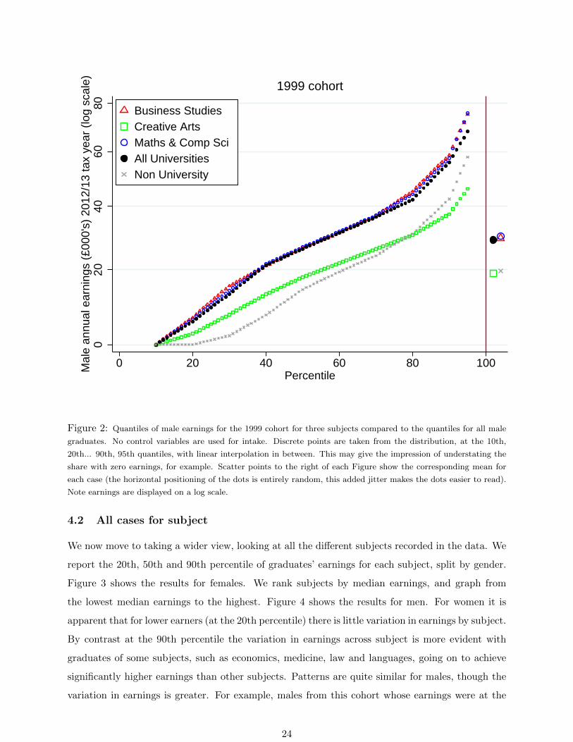
Figure 2: Quantiles of male earnings for the 1999 cohort for three subjects compared to the quantiles for all male

graduates. No control variables are used for intake. Discrete points are taken from the distribution, at the 10th,

20th... 90th, 95th quantiles, with linear interpolation in between. This may give the impression of understating the

share with zero earnings, for example. Scatter points to the right of each Figure show the corresponding mean for

each case (the horizontal positioning of the dots is entirely random, this added jitter makes the dots easier to read).

Note earnings are displayed on a log scale.

4.2 All cases for subject

We now move to taking a wider view, looking at all the different subjects recorded in the data. We

report the 20th, 50th and 90th percentile of graduates’ earnings for each subject, split by gender.

Figure 3 shows the results for females. We rank subjects by median earnings, and graph from

the lowest median earnings to the highest. Figure 4 shows the results for men. For women it is

apparent that for lower earners (at the 20th percentile) there is little variation in earnings by subject.

By contrast at the 90th percentile the variation in earnings across subject is more evident with

graduates of some subjects, such as economics, medicine, law and languages, going on to achieve

significantly higher earnings than other subjects. Patterns are quite similar for males, though the

variation in earnings is greater. For example, males from this cohort whose earnings were at the

24

90th percentile and who studied economics earned in excess of £120k, whilst those who studied

Creative Arts earned less than £40k at the 90th percentile. However, caution is needed when

interpreting these results since they take no account of the student intake into different subjects

and the fact that some subjects attract students with much higher levels of prior achievement.

020

4060

8010

012

0F

emal

e an

nual

ear

ning

s (£

000'

s) 2

012/

13 ta

x ye

ar

Cre

Art

s

Mas

s C

omm

Vet

, Agr

i

Mis

s O

ther

Soc

Sci

Mis

s LE

M

Mis

s S

TE

M

Bus

ines

s

Mat

h &

Com

p

Alli

ed m

ed

Arc

hite

ctur

e

Ling

Cla

ss

His

t Phi

l

Eng

& T

ech

Bio

Sci

Edu

catio

n

Phy

Sci

Law

Lang

Lit

Eco

nom

ics

Med

icin

e

20th Perc. No University (20th Perc.)Median No University (Median)90th Perc. No University (90th Perc.)

Figure 3: 20th, 50th, 90th percentile earnings for 1999 cohort female graduates in 2012/13 by subject. The area

of the solid blob indicates subject size. The crosses to the right of each Figure shows earnings at the 20th, 50th and

90th percentiles across all subjects.

25

020

4060

8010

012

0M

ale

annu

al e

arni

ngs

(£00

0's)

201

2/13

tax

year

Cre

Art

s

Mas

s C

omm

Vet

, Agr

i

Mis

s O

ther

Mis

s S

TE

M

Ling

Cla

ss

Lang

Lit

Bio

Sci

Soc

Sci

His

t Phi

l

Bus

ines

s

Mat

h &

Com

p

Mis

s LE

M

Alli

ed m

ed

Arc

hite

ctur

e

Edu

catio

n

Phy

Sci

Law

Eng

& T

ech

Eco

nom

ics

Med

icin

e

20th Perc. No University (20th Perc.)Median No University (Median)90th Perc. No University (90th Perc.)

Figure 4: 20th, 50th, 90th percentile earnings for 1999 cohort male graduates in 2012/13 by subject. The area of

the solid blob indicates subject size. The crosses to the right of each Figure shows earnings at the 20th, 50th and

90th percentiles across all subjects.

We now consider some conditional estimates that do take account of differences in student

characteristics across subjects. To account for prior achievement of students the left hand side of

Figure 5 shows the earnings of females by subject but this time conditional on other factors that

influence earnings, including age, region, parental income and the full set of HESA characteristics

(the method we use for this is described in more detail below). The latter are at subject-institution

level and include tariff score of intake. The right hand side of Figure 5 contains the results for

men. Once some account is taken of student and course characteristics, the variation in graduates’

earnings are reduced somewhat. Nonetheless the main findings still hold. There is little variation

by subject at the 20th percentile for males or females. At the 90th percentile subject matters more

for both genders and in particular graduates of medicine, law, economics and languages continue

to go on to achieve much higher earnings. However, it should be noted that we believe the model

we use for our conditioning is more accurate at the median than in the tails, meaning the 90th and

20th percentiles here should be treated with caution (the same does not apply for the unconditional

26

plots above).0

2040

6080

100

120

Fem

ale

annu

al e

arni

ngs

(£00

0's)

201

2/13

tax

year

Cre

Art

s

Mas

s C

omm

Vet

, Agr

i

Mis

s O

ther

Soc

Sci

Mis

s LE

M

Mis

s S

TE

M

Bus

ines

s

Mat

h &

Com

p

Alli

ed m

ed

Arc

hite

ctur

e

Ling

Cla

ss

His

t Phi

l

Eng

& T

ech

Bio

Sci

Edu

catio

n

Phy

Sci

Law

Lang

Lit

Eco

nom

ics

Med

icin

e

20th Perc. No University (20th Perc.)Median No University (Median)90th Perc. No University (90th Perc.)

Predictive model for Female earnings

020

4060

8010

012

0M

ale

annu

al e

arni

ngs

(£00

0's)

201

2/13

tax

year

Cre

Art

s

Mas

s C

omm

Vet

, Agr

i

Mis

s O

ther

Mis

s S

TE

M

Ling

Cla

ss

Lang

Lit

Bio

Sci

Soc

Sci

His

t Phi

l

Bus

ines

s

Mat

h &

Com

p

Mis

s LE

M

Alli

ed m

ed

Arc

hite

ctur

e

Edu

catio

n

Phy

Sci

Law

Eng

& T

ech

Eco

nom

ics

Med

icin

e

20th Perc. No University (20th Perc.)Median No University (Median)90th Perc. No University (90th Perc.)

Predictive model for Male earnings

Figure 5: Model based predicted earnings at the 20th, 50th and 90th percentiles for the 1999 cohort in 2012/13

by subject. Left is female, right is male. The predicted model includes controls for university characteristics at

the subject-institution level, age, parental income and region of the student, in addition to the control for year of

observation. The solid blob indicates the number of students taking that particular subject. The crosses to the right

of each Figure shows earnings at the 20th, 50th and 90th percentiles across all subjects.

5 Variation by institution

5.1 Some case studies of institutions

To start we again focus on three examples, a subset of the English universities that have kindly given

us permission to name them in our study. Our choices are University of Cambridge, Southampton

University and Warwick University.

In Figure 6 we show for each institution, annual female earnings for the 1999 cohort of graduates

in the tax year 2012/13 at each percentile in the earnings distribution. The earnings for graduates

from each institution are shown separately, along with earnings for graduates from all institutions

included for comparison (black dots), together with the earnings of non-graduates using the grey

crosses. There is considerably more variation across these institutions than we saw across the three

subjects in the previous section (note carefully the different scales).

The scatter points to the right of each figure show the mean annual earnings of graduates from

each institution and for all institutions. Overall it shows, of the three HEPs used here, graduates

from the University of Cambridge have the highest earnings for the upper part of the earnings

distribution, with more bunching across institutions at the 50 percentile level. There is much more

variation at the higher quantiles. The gaps between the universities seem more pronounced for men

than for women (recall the figures are drawn on the log scale), an effect which we will see holds up

for a wider set of HEPs.

27

To take an important snapshot, at the median earnings within each subgroup for females: non-

university earnings are £7.5k, all university earnings are £21.6k, while the universities highlighted

here scatter between £24.8k-£32.5k, including individuals with zero earnings in the calculations.

Hence, roughly, female graduate earnings are three times higher than non-university earnings, and

this group of institutions boosts earnings over all universities by another factor of 1.1-1.5.

At the 90% percentile the corresponding numbers are £34.9k, £44.2k and £50.8k-£71.5k.

Hence, the multiples are 1.3 and 1.1-1.6.

025

5010

015

020

0F

emal

e an

nual

ear

ning

s 20

12/1

3 ta

x ye

ar (

log

scal

e)

0 20 40 60 80 100Percentile

Cambridge SouthamptonWarwick All UniversitiesNon University

Figure 6: Quantiles of female earnings for the 1999 cohort from three of our case study universities compared to

the distribution for all female graduates. Discrete points are taken from the distribution, at the 10th, 20th... 90th,

95th quantiles, with linear interpolation in between. This may give the impression of understating the share with

zero earnings, for example. Points to the right of each figure show the mean for each case (the horizontal positioning

of the dots is entirely random, this added jitter makes them easier to read).

Figure 7 gives the corresponding results for men. Again the University of Cambridge has higher

earnings over the upper part of the distribution. If we focus on the median earnings within each

subgroup for males: non-university earnings are £14.4k, all university earnings are £26.3k, while

the universities highlighted here scatter between £29.5k-£38.7k. Hence, roughly, male graduate

earnings are roughly twice as high as non-university earnings, and this group boosts over all uni-

28

versities by another (multiplicative) factor of 1.1-1.5 (which very similar to the boost for women).

At the 90% percentile the corresponding numbers are £42.5k, £55.9k and £71.6k-£121.4k.

Hence, the multiples are 1.3 and 1.7-2.9, much greater than the corresponding multipliers for

women.

025

5010

015

020

0M

ale

annu

al e

arni

ngs

2012

/13

tax

year

(lo

g sc

ale)

0 20 40 60 80 100Percentile

Cambridge SouthamptonWarwick All UniversitiesNon University

Figure 7: Quantiles of male earnings for the 1999 cohort from three of our case study universities compared to the

distribution for all male graduates. Discrete points are taken from the distribution, at the 10th, 20th... 90th, 95th

quantiles, with linear interpolation in between. This may give the impression of understating the share with zero

earnings, for example. Points to the right of each figure show the mean for each case (the horizontal positioning of

the dots is entirely random, this added jitter makes them easier to read).

Each of the three named institutions have graduates with higher earnings than the average

for graduates from all institutions, at least from the 40th percentile upwards. This observation

is not surprising, as we have named institutions that have a more academically selective intake

and therefore are likely to admit students who would have better earnings prospects than average,

irrespective of their higher education institution. Further, within the sample of institutions there is

variation in student intake, the balance of subjects offered and region in which the HEP is located.

All these factors can dramatically influence the unconditional earnings distributions that we

show in Figures 6 and 7 and might make direct comparisons of institutions using the level of

29

earnings of students misleading if we are interested in the value added by each institution. For

example, graduates from Cambridge have the highest earnings for the upper parts of the earnings

distribution. This is likely to be partially explained by its economically advantageous location and

highly selective student intake.

To start to address this issue we build a predictive model for the earnings distribution at

each institution by gender. This is done in two-step process. First, we “correct” the earnings

for each institution using a pooled regression of earnings on a set of demeaned characteristics

including subject studied, region applied from, whether or not the individual is from a higher

income household and the HESA controls. Our corrected earnings are then the residuals from

this regression. Second, we re-estimate the model described in section 3 with Yi,t replaced with

corrected earnings.

Figure 8 shows these corrected earnings for each of our three case study universities. The

figure shows that much of the differences between institutions is expected when we account for the

differences in these background variables that influence earnings. This is perhaps most obvious

when looking at the scatter plots of means which indicate the compression in mean annual earnings

differences across institutions in the conditional plots. In other words, mean differences in earnings

across most institutions are not sizeable once we take account of the fact that different types of

student sort into different institutions.

Of course, this exercise is limited. In particular, the tariff scores are pretty coarse measures

of pre-HE performance, particularly at the higher level of achievement. Admissions officers at

HEPs have a broader set of quantitative and qualitative information with which to select students.

This means our conditional approach is likely to be only an approximate way to calibrate expected

performance of HEPs. Further, we again note that we believe the model we use for our conditioning

is more accurate towards the middle of the distribution than in the tails.

30

025

5010

015

020

0F

emal

e an

nual

ear

ning

s (£

000'

s) 2

012/

13 ta

x ye

ar (

log

scal

e)

0 20 40 60 80 100Percentile

Cambridge SouthamptonWarwick All Universities

025

5010

015

020

0M

ale

annu

al e

arni

ngs

(£00

0's)

201

2/13

tax

year

(lo

g sc

ale)

0 20 40 60 80 100Percentile

Cambridge SouthamptonWarwick All Universities

Figure 8: Model based predicted earnings for the 1999 cohort from three of our case study universities compared to

the distribution for all graduates, by gender. The predicted model uses an additive model based on the variables: the

mean UCAS tariff of the institution, parental income, subject dummy variables and region of institution. Discrete

points are taken from the distribution, at the 10th, 20th... 90th, 95th quantiles, with linear interpolation in between.

This may give the impression of understating the share with zero earnings, for example. Points to the right of each

figure show the mean for each case (the horizontal positioning of the dots is entirely random, this added jitter makes

them easier to read).

5.2 All institutions

Figure 9 shows the 20th, 50th and 90th percentile earnings for the female 1999 cohort observed

in 2012/13 displayed for each institution for which we have sufficient data to report estimates.

Figure 11 shows the same information for male graduates. Universities are ranked left to right on

their graduates’ 2012/13 median earnings (hence the green line of dots looks smooth).9 This shows

unconditional earnings by institution at the different parts of the earnings distribution.

Our named institutions are included for illustrative purposes.10 They are displayed with a

fuller colour and are numbered, while we have faded the colours from the other HEPs. Each of

these named universities have results which appear in the top third of our median income ranking.

They are magnified in Figures 10 and 12 which focuses on this top third to make it easier to read.

One notable observation is the very strong performance of some northern universities, Liverpool,

Newcastle and York, which have graduates that achieve highly competitive earnings even though

their local labour markets have lower earnings than we see in the southern part of England. Also

note the strong levels of earnings of the London based HEPs: Imperial, LSE and Kings. LSE

additionally benefits from focusing also on high paying subjects, Economics and Law, as well as

having very high admissions requirements. Taken together, both female and male LSE graduates

9This should not be considered as comparable to the numerous rankings of universities that are currently availablein the UK, and is simply used to make the Figures easier to read. There is no attempt here to allow for subject ofstudent composition, for example.

10We reiterate here that our estimates are for those domiciled in England upon application. This is a select sample,therefore, in particular for Cardiff and Edinburgh universities, as the majority of their students were domiciled uponapplication in Wales and Scotland respectively.

31

are some of the very highest earnings graduates in the country.

4

15

1410 16

1512 17

2

3

613117

9

8

4

15

14 10

1615

12

17

23 613

117

9

8

4

1

5

1410

1615

12

17

23

613

11

7

9

8

1 = Cambridge2 = Manchester3 = Newc4 = Bristol5 = Cardiff6 = Nottingham

7 = Southampton8 = York9 = Warwick10 = Exeter11 = Oxford12 = Liverpool

13 = Durham14 = Edinburgh15 = Kings16 = Imperial17 = LSE

030

6090

120

150

180

Fem

ale

annu

al e

arni

ngs

(£00

0's)

201

2/13

tax

year

HEP ranked on median annual earnings

20th Perc. Median90th Perc. No University (20th Perc.)No University (Median) No University (90th Perc.)

Figure 9: Unconditional female 20th, 50th and 90th percentile earnings for the 1999 cohort in2012/13 for HEPs ranked on their graduates’ 2012/13 median earnings. There are 166 differentinstitutions included, and one “other” institution which include several hundred institutions thatissue only a handful of loans. Note: The log scale is not used here. Zeros are included.

32

4

15

1410 16

1512 17

2

3

613117

9

8

4

15

14 10

1615

12

17

23 613

117

9

8

4

1

5

1410

1615

12

17

23

613

11

7

9

8

1 = Cambridge2 = Manchester3 = Newc4 = Bristol5 = Cardiff6 = Nottingham

7 = Southampton8 = York9 = Warwick10 = Exeter11 = Oxford12 = Liverpool

13 = Durham14 = Edinburgh15 = Kings16 = Imperial17 = LSE

030

6090

120

150

180

Fem

ale

annu

al e

arni

ngs

(£00

0's)

201

2/13

tax

year

HEP ranked on median annual earnings

20th Perc. Median90th Perc. No University (20th Perc.)No University (Median) No University (90th Perc.)

Figure 10: Top third of Figure 9. Unconditional female 20th, 50th and 90th percentile earnings forthe 1999 cohort in 2012/13 for HEPs ranked on their graduates’ 2012/13 median earnings. Thisis a repeat of Figure 9, zoomed in on the top one third of HEPs. Note: The log scale is not usedhere. Zeros are included.

33

4

15

1410 16

1512 172

36

1311

7

9

8

4

15

14 1016

15

12

17

2

3 613

11

7

9

8

4

1

514

10

16 15

12

17

2

3 6

13

11

79

8

1 = Cambridge2 = Manchester3 = Newc4 = Bristol5 = Cardiff6 = Nottingham

7 = Southampton8 = York9 = Warwick10 = Exeter11 = Oxford12 = Liverpool

13 = Durham14 = Edinburgh15 = Kings16 = Imperial17 = LSE

030

6090

120

150

180

Mal

e an

nual

ear

ning

s (£

000'

s) 2

012/

13 ta

x ye

ar

HEP ranked on median annual earnings

20th Perc. Median90th Perc. No University (20th Perc.)No University (Median) No University (90th Perc.)

Figure 11: Unconditional male 20th, 50th and 90th percentile earnings for the 1999 cohort in2012/13 for HEPs ranked on their graduates’ 2012/13 median earnings. There are 168 differentinstitutions included, and one “other” institution which include several hundred institutions thatissue only a handful of loans. Note: The log scale is not used here. Zeros are included.

34

4

15

1410 16

1512 172

36

1311

7

9

8

4

15

14 1016

15

12

17

2

3 613

11

7

9

8

4

1

514

10

16 15

12

17

2

3 6

13

11

79

8

1 = Cambridge2 = Manchester3 = Newc4 = Bristol5 = Cardiff6 = Nottingham

7 = Southampton8 = York9 = Warwick10 = Exeter11 = Oxford12 = Liverpool

13 = Durham14 = Edinburgh15 = Kings16 = Imperial17 = LSE

030

6090

120

150

180

Mal

e an

nual

ear

ning

s (£

000'

s) 2

012/

13 ta

x ye

ar

HEP ranked on median annual earnings

20th Perc. Median90th Perc. No University (20th Perc.)No University (Median) No University (90th Perc.)

Figure 12: Top third of Figure 11. Unconditional male 20th, 50th and 90th percentile earnings forthe 1999 cohort in 2012/13 for universities ranked on their graduates’ 2012/13 median earnings.This is a repeat of Figure 11, zoomed in on the top one third of HEPs. Note: The log scale is notused here. Zeros are included.

Figures 10 and 12 repeat the previous figures but focus solely on the top third of institutions

to make reading the figures somewhat easier.

To provide some context for the display of graduates’ earnings, the average for non-graduates

at the 20th, 50th and 90th percentiles is indicated by a cross and associated dashed line. What

is perhaps most interesting is the sheer quantity of variation in graduates’ earnings within an

institution. The earnings of male graduates from the LSE for example are around £163k at the

90th percentile but at the median are nearer £45k while at the bottom 20th percentile the figure

is close to zero. The figures also illustrate the large gender gap prevalent for many institutions,

particularly at the top end of the earnings distribution.

Another striking feature of the data is the very low earnings of graduates from most institutions

at the 20th percentile of the distribution. We noted already that these data include graduates with

zero and low earnings, including those working part time or indeed not working at all (whether

by choice, e.g. taking more training, or due to unemployment). A significant proportion of the

35

graduate labour market is therefore low earning (noting that graduates who are abroad appear as

having zero earnings in our data), irrespective of institution, but in these data we are unable to say

why that might be. However, to put this in context, this low earning share is lower than we see in

the non-university population.

Note that we observe a similar pattern for males and females and hence this feature of the

data cannot be entirely explained by women choosing to stay out of the labour market in larger

numbers. Given previous evidence that lower income students are less likely to access Russell Group

institutions which appear to be higher ranking in terms of their graduates’ earnings, a major issue

for those concerned with improving social mobility is the extent to which students from lower

income families are disproportionately likely to be found in these groups of much lower earning

graduates.

Another striking feature is the substantial earnings of graduates at the 90th percentile across

a large number of institutions. Graduates from all our named institutions earn £60k or above at

the 90th percentile of the distribution and even at very low ranked institutions graduates at the

90th percentile earn £30k or more, even including graduates with zero earnings. Further these

data illustrate the earnings advantage of graduates as compared to non-graduates. Almost all

institutions have graduates with earnings above the 20th percentile of the non-graduate earnings

distribution, and most institutions have graduates with earnings above the non-graduate median.

At the other end of the spectrum, there were some institutions (23 for men and 9 for women)

where the median graduate earnings were less than those of the median non-graduate ten years on.

It is important to put this in some context though. Many English higher education institutions

draw a significant majority of their students from people living in their own region. Given regional

differences in average wages, some very locally focused institutions may struggle to produce grad-

uates whose wages outpace England-wide earnings, which include those living in London etc. To

illustrate regional differences, employment rates in the period under consideration varied between

66% in the North East and 75% in the East of England, and data from the Annual Survey of Hours

and Earnings suggests that average full-time earnings for males were approximately 48% higher

in London than in Northern Ireland, and around 34% higher for females. Regional differences are

therefore important and we take them into account in our analysis of graduates’ earnings. However,

we cannot construct a more natural benchmark for these locally focused institutions, such as an

estimate of the quantiles of the earnings of non-university people in their region, because the data

we received from HMRC on non-graduates do not have that regional indicator and so we are unable

to carry out that comparison.

As discussed earlier we are conscious that the earnings of graduates from different institutions

36

will vary because of the student intake or subject mix at that particular institution. Figure 13

provides the predictive estimates of differences in graduates’ earnings by institution and suggests

significant compression of the differences by institution once account is taken of other factors that

influence earnings, such as student intake. Certainly institutional variation at the 20th and 50th

percentiles is much reduced. There continues to be outlier institutions with very high earnings at

the 90th percentile, although we again note that we believe the model we use for our conditioning

is more accurate at the median than in the tails, meaning the 90th and 20th percentiles here should

be treated with caution (the same does not apply for the unconditional plots above). It also shows

the rankings of the named institutions remain roughly similar even after controlling for differences

in other variables that influence earnings.

415

14 10 16

1512 172

3

613 1179

8

41

5

14 10 16

1512

17

23

613 1179

8

41

5

14 10

1615

12

17

23

613

11

79

8

1 = Cambridge2 = Manchester3 = Newc4 = Bristol5 = Cardiff6 = Nottingham

7 = Southampton8 = York9 = Warwick10 = Exeter11 = Oxford12 = Liverpool

13 = Durham14 = Edinburgh15 = Kings16 = Imperial17 = LSE

030

6090

120

150

180

Fem

ale

annu

al e

arni

ngs

(£00

0's)

201

2/13

tax

year

HEP ranked on median annual earnings

20th Perc. Median90th Perc. No University (20th Perc.)No University (Median) No University (90th Perc.)

41

5

1410

161512 17

2

36

13

1179

8

41

5

14 10 16

15

12

17

2

36

1311

79

8

4

1

51410

16 15

12

17

2

3

6

13

11

7 9

8

1 = Cambridge2 = Manchester3 = Newc4 = Bristol5 = Cardiff6 = Nottingham

7 = Southampton8 = York9 = Warwick10 = Exeter11 = Oxford12 = Liverpool

13 = Durham14 = Edinburgh15 = Kings16 = Imperial17 = LSE

030

6090

120

150

180

Mal

e an

nual

ear

ning

s (£

000'

s) 2

012/

13 ta

x ye

ar

HEP ranked on median annual earnings

20th Perc. Median90th Perc. No University (20th Perc.)No University (Median) No University (90th Perc.)

Figure 13: Predictive 20th, 50th and 90th percentile earnings for the 1999 cohort in 2012/13 foruniversities ranked on their graduates’ 2012/13 median earnings. The predicted model uses anadditive model based on the variables: the mean UCAS tariff of the institution, parental income,subject mix and region of institution. Non-university is included as a reference point, but note thatthese reflect unconditional earnings figures as the predictive model is not applied to this group.Note: The log scale is not used here. Ranking of institutions is based on estimated unconditionalmedian earnings, not their predicted earnings.

5.3 Earnings Growth

Thus far we have focused on earnings variation at one point in time for a particular cohort. Our

data also enable us to look at the development of graduates’ earnings over time as they progress

in their career. Figure 14 gives some insight into how the earnings of graduates from the 1999

cohort develop over the period 2008/09-2012/13, shown separately by gender (a similar figure for

the 2002 cohort is in the appendix to this paper). We show earnings for all graduates, non graduates

and graduates from our case study institutions. It is of course important to note that the period

we consider here coincides with the 2008 economic recession and its aftermath, where across the

37

economy real earnings fell quite dramatically. This fall in real earnings particularly impacted the

relatively young, such as those we are studying here. Thus this figure will be unlikely to be a

representative period. The figure shows flat earnings with minimal growth for non graduates and

female graduates but even in this period of economic turbulence, male graduates saw some growth

and in particular male graduates from our case study institutions saw appreciable earnings growth.

It appears that for males at least, attending a high status university did offer some protection from

the impact of the recent recession.

010

2030

4050

Ann

ual e

arni

ngs

(£00

0's)

2009 2010 2011 2012 2013year

Case studies Female Case studies MaleAll unis Female All Unis MaleNo Uni Female No Uni Male

Figure 14: Mean earnings (including zeros) for a given cohort over time, by gender. This shows the 1999 cohort

for 2008/09-2012/13.

6 Variation in earnings by subject and institution

We now turn to investigating the interaction between institution and subject to see if going to top

institutions immunises the student against low earnings associated with certain subjects. We show

that the answer varies by subject: there are subjects where institutions matter a great deal, others

where it is not very relevant. We also show that for some institutions, subject choice really does

matter, while for others, less so. In general, the choice of broader subject grouping (LEM, STEM

or OTHER) appears to matter more than the choice between individual subjects.

6.1 Institutions and subject groups

We start by combining subjects into the aggregate subject groups described earlier, namely Law,

Economics and Management (LEM); Science, Technology, Engineering and Mathematics (STEM)

38

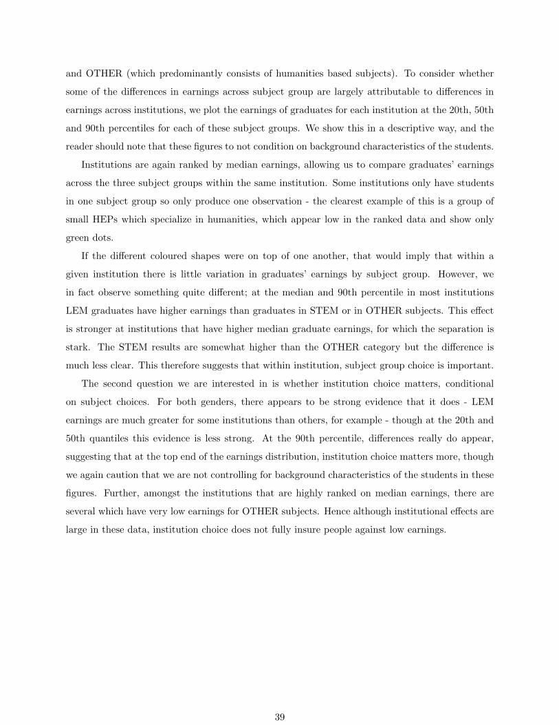
and OTHER (which predominantly consists of humanities based subjects). To consider whether

some of the differences in earnings across subject group are largely attributable to differences in

earnings across institutions, we plot the earnings of graduates for each institution at the 20th, 50th

and 90th percentiles for each of these subject groups. We show this in a descriptive way, and the

reader should note that these figures to not condition on background characteristics of the students.

Institutions are again ranked by median earnings, allowing us to compare graduates’ earnings

across the three subject groups within the same institution. Some institutions only have students

in one subject group so only produce one observation - the clearest example of this is a group of

small HEPs which specialize in humanities, which appear low in the ranked data and show only

green dots.

If the different coloured shapes were on top of one another, that would imply that within a

given institution there is little variation in graduates’ earnings by subject group. However, we

in fact observe something quite different; at the median and 90th percentile in most institutions

LEM graduates have higher earnings than graduates in STEM or in OTHER subjects. This effect

is stronger at institutions that have higher median graduate earnings, for which the separation is

stark. The STEM results are somewhat higher than the OTHER category but the difference is

much less clear. This therefore suggests that within institution, subject group choice is important.

The second question we are interested in is whether institution choice matters, conditional

on subject choices. For both genders, there appears to be strong evidence that it does - LEM

earnings are much greater for some institutions than others, for example - though at the 20th and

50th quantiles this evidence is less strong. At the 90th percentile, differences really do appear,

suggesting that at the top end of the earnings distribution, institution choice matters more, though

we again caution that we are not controlling for background characteristics of the students in these

figures. Further, amongst the institutions that are highly ranked on median earnings, there are

several which have very low earnings for OTHER subjects. Hence although institutional effects are

large in these data, institution choice does not fully insure people against low earnings.

39

050

100

150

200

250

300

350

Fem

ale

annu

al e

arni

ngs

(£00

0's)

201

2/13

tax

year

HEP ranked on median annual earnings

LEM OtherSTEM No University

Females, 20th percentile

050

100

150

200

250

300

350

Mal

e an

nual

ear

ning

s (£

000'

s) 2

012/

13 ta

x ye

ar

HEP ranked on median annual earnings

LEM OtherSTEM No University

Males, 20th percentile

050

100

150

200

250

300

350

Fem

ale

annu

al e

arni

ngs

(£00

0's)

201

2/13

tax

year

HEP ranked on median annual earnings

LEM OtherSTEM No University

Females, 50th percentile

050

100

150

200

250

300

350

Mal

e an

nual

ear

ning

s (£

000'

s) 2

012/

13 ta

x ye

ar

HEP ranked on median annual earnings

LEM OtherSTEM No University

Males, 50th percentile

050

100

150

200

250

300

350

Fem

ale

annu

al e

arni

ngs

(£00

0's)

201

2/13

tax

year

HEP ranked on median annual earnings

LEM OtherSTEM No University

Females, 90th percentile

050

100

150

200

250

300

350

Mal

e an

nual

ear

ning

s (£

000'

s) 2

012/

13 ta

x ye

ar

HEP ranked on median annual earnings

LEM OtherSTEM No University

Males, 90th percentile

Figure 15: 20th, 50th and 90th percentile earnings by subject group. Note: the ranking of carriedout by overall estimated median earnings of HEP, not by subject-specific median.

40

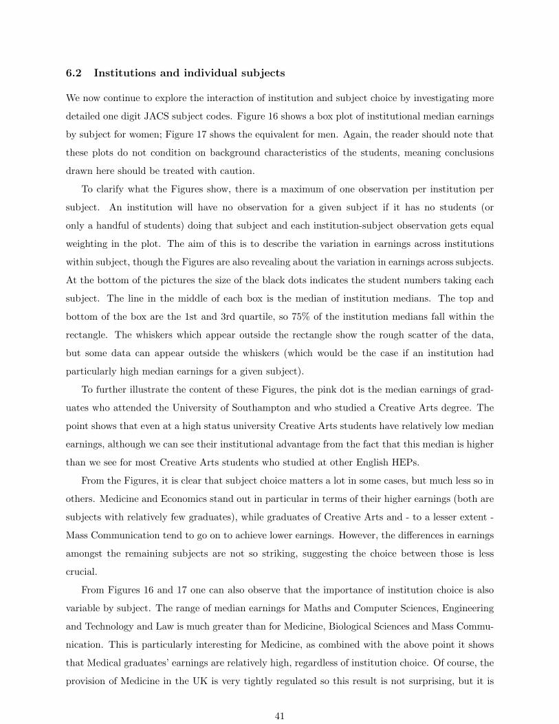
6.2 Institutions and individual subjects

We now continue to explore the interaction of institution and subject choice by investigating more

detailed one digit JACS subject codes. Figure 16 shows a box plot of institutional median earnings

by subject for women; Figure 17 shows the equivalent for men. Again, the reader should note that

these plots do not condition on background characteristics of the students, meaning conclusions

drawn here should be treated with caution.

To clarify what the Figures show, there is a maximum of one observation per institution per

subject. An institution will have no observation for a given subject if it has no students (or

only a handful of students) doing that subject and each institution-subject observation gets equal

weighting in the plot. The aim of this is to describe the variation in earnings across institutions

within subject, though the Figures are also revealing about the variation in earnings across subjects.

At the bottom of the pictures the size of the black dots indicates the student numbers taking each

subject. The line in the middle of each box is the median of institution medians. The top and

bottom of the box are the 1st and 3rd quartile, so 75% of the institution medians fall within the

rectangle. The whiskers which appear outside the rectangle show the rough scatter of the data,

but some data can appear outside the whiskers (which would be the case if an institution had

particularly high median earnings for a given subject).

To further illustrate the content of these Figures, the pink dot is the median earnings of grad-

uates who attended the University of Southampton and who studied a Creative Arts degree. The

point shows that even at a high status university Creative Arts students have relatively low median

earnings, although we can see their institutional advantage from the fact that this median is higher

than we see for most Creative Arts students who studied at other English HEPs.

From the Figures, it is clear that subject choice matters a lot in some cases, but much less so in

others. Medicine and Economics stand out in particular in terms of their higher earnings (both are

subjects with relatively few graduates), while graduates of Creative Arts and - to a lesser extent -

Mass Communication tend to go on to achieve lower earnings. However, the differences in earnings

amongst the remaining subjects are not so striking, suggesting the choice between those is less

crucial.

From Figures 16 and 17 one can also observe that the importance of institution choice is also

variable by subject. The range of median earnings for Maths and Computer Sciences, Engineering

and Technology and Law is much greater than for Medicine, Biological Sciences and Mass Commu-

nication. This is particularly interesting for Medicine, as combined with the above point it shows

that Medical graduates’ earnings are relatively high, regardless of institution choice. Of course, the

provision of Medicine in the UK is very tightly regulated so this result is not surprising, but it is

41

010

2030

4050

6070

80F

emal

e an

nual

ear

ning

s (£

000'

s) 2

012/

13 ta

x ye

ar

Med

icin

e

Alli

ed M

ed

Bio

Sci

Vet

, Agr

i

Phy

Sci

Mat

h &

Com

p

Eng

& T

ech

Arc

hite

ctur

e

Soc

Sci

Eco

nom

ics

Law

Bus

ines

s

Mas

s C

omm

Ling

Cla

ss

Lang

& L

it

His

t & P

hil

Cre

Art

s

Edu

c

Mis

s S

TE

M

Mis

s LE

M

Mis

s O

ther

Female

Figure 16: Box plots showing variation in institution-level median earnings at subject level forwomen for the 1999 cohort in 2012/13. Area of the blob size indicates number of students. Thepink dot is for illustrative purposes, showing the median earnings of former graduates from theUniversity of Southampton who studied Creative Arts.

42

010

2030

4050

6070

80M

ale

annu

al e

arni

ngs

(£00

0's)

201

2/13

tax

year

Med

icin

e

Alli

ed M

ed

Bio

Sci

Vet

, Agr

i

Phy

Sci

Mat

h &

Com

p

Eng

& T

ech

Arc

hite

ctur

e

Soc

Sci

Eco

nom

ics

Law

Bus

ines

s

Mas

s C

omm

Ling

Cla

ss

Lang

& L

it

His

t & P

hil

Cre

Art

s

Edu

c

Mis

s S

TE

M

Mis

s LE

M

Mis

s O

ther

Male

Figure 17: Box plots showing variation in institution-level median earnings at subject level for menfor the 1999 cohort in 2012/13. Area of the blob size indicates number of students.

43

impactful. The same cannot be said for Economics graduates, for whom the returns appear to be

high in expectation, but much less certain, while the opposite holds true for Creative arts and Mass

Communication: both the level and variation in earnings for these subjects is low. In fact in terms

of subsequent graduate earnings for both, even the relatively high achieving institutions (at the

75th percentile) are dominated by the relatively low achieving institutions (at the 25th percentile)

for Medicine and Economics for both genders.

6.3 Institutions and individual subjects: model results

So far in this section we have investigated the importance of both subject choice conditional on

institution and institution choice conditional on subject. However, thus far we have only displayed

this without conditioning on important background characteristics. In this sub-subsection, we

investigate these questions using more formal regression analysis.

Table 9 quantifies the differences in median graduate earnings for different subjects. The purpose

of this table is to illustrate how median earnings vary by subject even after allowing for other

sources of variation in earnings, namely student and institution characteristics. It relies on data

from 2011/12 and 2012/13 for the 1999 cohort. Specifically, columns 1 and 2 shows the coefficients

on subject dummy variables from a median regression of earnings with no additional controls (other

than indicators of the year of the data) for females and males respectively. The results in these

columns can therefore be interpreted as the raw or unconditional differences in earnings by subject,

showing for example that the estimated median earnings for male (female) graduates in Medicine

is around £51k (£41k) whilst for male (female) graduates in Creative Arts it is around £17k

(£12k). The earnings variation across subjects is quite stark. To illustrate more concretely the

variation in earnings that appears to be attributable to subject, in Columns 3 and 4 we present

the earnings premiums for each subject relative to the earnings that graduates in the Creative Arts

earn (Creative Arts was selected as it has a large student body and has low earnings). Hence male

(female) graduates in Medicine have median earnings that are around £34k (£29k) greater than

those with Creative Arts degrees.

Next we present results from the same model as previously but with additional controls for age,

region, parental income and higher education fixed effects included. Again to illustrate the impact

of these controls we show the earnings premiums for each subject compared to the earnings for

Creative Arts. After these controls are added the premiums associated with Medicine for males

(females) is substantially lower at £24k (£23k). Hence some of the higher premiums that Medicine

attracts is attributable to other factors, including the fact that Medicine is studied at high tariff

institutions. Nonetheless even after allowing for these factors, medical graduates earn significantly

more than those from other subjects.

44

After allowing for these characteristics, the earnings premiums associated with some subjects is

reduced. For instance, the premium associated with Economics for males (females) is reduced from

£23k (£20k) to £13k (£18k). Again this indicates that the high premium for Economics is partly

attributable to other factors, including the institutions that offer this subject. This specification

does not however control for the student intake in that particular subject at that specific institution,

which may differ from the average student intake at that institution as a whole. In the final two

columns we control for the subject/institution characteristics using HESA data, including the tariff

points of students in that subject/institution combination. We have to remove institution fixed

effects to enable the model to converge. The pattern of results does not change markedly though the

coefficients on medicine are reduced somewhat and some subject differences that were previously

statistically insignificant become marginally so and vice versa. In summary, the differences in

earnings across subjects get compressed once we take account of the fact that graduates with

different characteristics take different degree subjects at different institutions. Therefore, although

part of the reason why Creative Arts graduates have very low earnings is because they possess

characteristics that would be associated with lower earnings anyway, this does not explain away

all of the earnings differences. This suggests that for a given individual it still holds true that the

subject choice between creative arts and the rest remains important.

45

Subject Subject Raw Raw Conditional ConditionalGroup earnings differences differences differences

(£000’s) from Cre Arts from Cre Arts from Cre Arts(£000’s) HEP f.e. HESA

(£000’s) (£000’s)

M F M F M F M FMedicine STEM 50.7 41.1 34.1∗∗∗ 28.6∗∗∗ 24.1∗∗∗ 23.2∗∗∗ 21.0∗∗∗ 21.8∗∗∗

2.8 4.7 4.2 5.6 8.3 7.8 4.2 4.9

Economics LEM 39.9 32.6 23.3∗∗∗ 20.1∗∗∗ 13.2 17.8∗∗ 13.9∗∗∗ 20.04.6 3.0 5.5 4.2 8.8 7.2 4.8 16.3

Eng & Tech STEM 29.1 19.8 12.5∗∗∗ 7.4∗ 6.4 5.1 7.9∗ 6.13.2 3.1 4.5 4.3 8.1 6.6 4.1 4.9

Educ Other 28.0 21.3 11.4∗∗ 8.9∗∗ 9.1 7.9 10.0∗∗ 8.7∗

3.4 3.1 4.6 4.4 8.2 7.2 4.0 4.8

Law LEM 28.0 23.3 11.3∗∗ 10.9∗∗ 7.1 8.7 7.1∗ 7.8∗

3.5 3.0 4.7 4.3 8.1 7.0 4.1 4.7

Phy Sci STEM 27.7 21.2 11.0∗∗ 8.7∗ 3.5 6.4 4.8 6.03.1 3.7 4.4 4.8 8.2 7.5 3.9 4.9

Architecture Other 26.4 17.6 9.8∗∗ 5.1 6.4 5.2 6.8 3.33.1 3.8 4.4 4.9 8.1 7.2 4.7 4.7

Allied Med STEM 26.4 21.3 9.8∗∗ 8.9∗∗ 6.0 7.3 6.6∗ 7.73.2 3.0 4.5 4.3 8.0 7.0 3.9 4.7

Lang & Lit Other 26.3 23.8 9.7∗∗ 11.3∗∗ 2.5 4.8 1.3 4.73.2 4.0 4.5 5.1 8.2 7.6 3.9 6.4

Math & Comp STEM 25.9 20.4 9.2∗∗ 8.0∗ 6.3 6.7 7.1∗ 7.03.2 2.8 4.5 4.2 8.1 6.7 4.0 4.7

Miss LEM LEM 25.8 18.5 9.2∗ 6.1 8.3 6.2 6.6 6.13.5 3.1 4.7 4.3 8.1 7.3 4.2 4.9

Business LEM 24.9 20.0 8.3∗ 7.5∗ 5.9 6.6 6.1 6.13.4 3.2 4.6 4.4 8.1 7.2 4.0 4.7

Hist & Phil Other 24.6 20.8 7.9∗∗ 8.4∗ 1.6 4.5 2.1 3.32.3 3.6 3.9 4.7 8.2 7.4 3.8 4.8

Soc Sci Other 24.5 18.4 7.9∗ 6.0 4.2 4.9 4.5 5.23.3 2.9 4.6 4.2 8.2 6.9 4.0 4.7

Bio Sci STEM 22.8 21.9 6.1 9.5∗∗ 1.1 6.0 2.0 5.93.2 3.5 4.5 4.6 8.2 7.4 4.1 4.8

Miss STEM STEM 21.9 18.3 5.3 5.8 4.2 5.0 4.0 3.93.6 3.5 4.7 4.6 8.1 7.0 4.1 5.1

Ling Class Other 21.6 20.8 4.9 8.3∗ -.9 4.8 -.1 4.63.5 3.1 4.7 4.4 8.5 7.0 4.6 4.7

Miss Other Other 21.2 17.3 4.6 4.9 4.7 5.6 4.5 5.03.2 3.0 4.5 4.3 8.1 7.0 4.1 4.8

Mass Comm Other 20.9 15.4 4.2 2.9 3.7 2.8 3.5 2.03.9 3.0 5.0 4.3 8.1 7.0 4.2 4.7

Vet, Agri STEM 20.1 18.2 3.5 5.8 4.3 4.8 4.2 5.54.0 3.3 5.1 4.5 8.1 7.3 4.9 4.9

Cre Arts Other 16.7 12.43.1 3.0

Years Yes Yes Yes Yes Yes Yes Yes YesRegions No No No No Yes Yes Yes YesAge No No No No Yes Yes Yes YesRich No No No No Yes Yes Yes YesHEI No No No No Yes Yes No NoHESA No No No No No No Yes YesN 21,184 24,058 21,184 24,058 21,184 24,058 21,184 24,058

Table 9: Subject median regressions. The first two columns of results show raw estimated earnings by subject. Thenext two show the difference in earnings from Creative Arts. The next two columns show the conditional differencesfrom Creative Arts - i.e. the differences once controls for region, age, parental income and HEI fixed effects areincluded. The final two columns show differences from Creative Arts with controls for region, age, parental incomeand HESA data included. All figures are in £000’s. Uses 2011/12 and 2012/13 data and the 1999 cohort (estimatesare given for 2012/13). Standard errors are clustered at HEP level. * indicates significantly different to the base(CreArts) at 10% level, ** 5% and *** 1%.

46

Whilst Table 9 quantifies the differences in graduates’ earnings associated with different degree

subjects, Table 10 shows the differences in median graduate earnings associated with different types

of institution. The purpose of this table is to illustrate how median earnings vary by institution

group (categorised by decile of mean UCAS tariff), even after allowing for other sources of differences

in earnings, namely student characteristics and subject of degree. The tables use data from 2011/12

and 2012/13, and presents estimated earnings for the 1999 cohort specifically.

Columns 1 and 2 provide estimates of median graduate earnings by institution group for females

and males respectively, from a median regression which controls only for year of observation. The

variation in median earnings across institution group is sizeable, with estimated male median

earnings ranging from around £20k for those in institutions in the lowest two decile groups through

to nearly £40k for those in the top 5 institutions. For women the variation is somewhat lower,

ranging from £15k for those in institutions in the bottom two decile groups through to £26k for

those in the top decile group. Further, for males there is a sizeable gap in earnings between those

in the top 5 institutions and those in the rest of the top decile group. For women, the earnings of

those in the top 5 institutions are not any higher than those in the rest of the top decile group.

Columns 3 and 4 follow the pattern from Table 9 and present the earnings premiums for females

and males respectively compared to the earnings of graduates in group G0. The results indicate

that median male (female) earnings in the top 5 institutions is around £18k (£11k) more than

those in the bottom two decile institution groups.

In the columns 4 and 5 the model includes controls for demographic factors (cohort, region, age,

rich, and subject fixed effects) but does not take account of the characteristics of the student intake

from the HESA data. In columns 4 and 5 it is apparent that much of the variation that appears

to be across institutions can be attributable to other factors. The median male (female) earnings

premium associated with being in a top 5 institution is reduced to £14k (£9k) compared to the

earnings of graduates in the bottom two decile institution groups. The final two columns then

add in controls for the HESA characteristics, including the mean tariff of the student intake. The

coefficients remain similar in magnitude in most cases, suggesting a premium for those attending

institutions in the top groups but the magnitude of the standard errors increases dramatically and

results become statistically insignificant. We conclude that there is clearly less variation in graduate

median earnings by institution group once one takes account of student characteristics and degree

subject. However for males, institution of study may be potentially an important determinant of

median earnings for those in the top groups but the methodology and quantity of data we use in

this model does not enable us to give sufficient precision to these estimates.

47

HEP Raw Raw Conditional ConditionalGroup earnings differences differences differences

(£000’s) from G0 from G0 from G0£000’s Subject HESA

(£000’s) (£000’s)

M F M F M FG10high 38.7 26.8 17.9∗∗∗ 10.6∗∗∗ 13.5∗∗∗ 8.4∗∗∗ 13.0 3.2

1.1 1.0 3.0 2.9 3.2 1.8 9.9 10.7

G10low 33.0 26.1 12.2∗∗∗ 9.8∗∗∗ 9.5∗∗∗ 7.3∗∗∗ 11.6 4.72.0 1.8 3.4 3.3 3.4 2.2 9.7 10.8

G9 31.4 25.5 10.6∗∗∗ 9.3∗∗∗ 7.2∗∗ 7.4∗∗∗ 9.1 5.61.5 1.2 3.2 3.0 3.2 1.7 9.7 10.6

G8 29.3 23.5 8.4∗∗∗ 7.3∗∗ 5.9∗ 6.4∗∗∗ 8.3 6.21.5 1.3 3.2 3.0 3.3 1.8 9.8 10.6

G7 28.5 21.3 7.7∗∗ 5.0 5.5∗ 4.5∗∗ 7.9 5.81.7 1.7 3.3 3.2 3.2 2.1 9.8 10.7

G6 24.7 19.7 3.8 3.5 3.8 4.1∗∗ 6.6 6.21.9 1.5 3.4 3.1 3.2 1.9 9.8 10.6

G5 23.8 19.9 3.0 3.7 2.8 3.8∗∗ 5.6 6.01.6 1.3 3.2 3.0 3.3 1.7 9.9 10.4

G4 22.2 17.6 1.4 1.3 1.7 2.9∗ 6.0 6.01.4 1.2 3.2 3.0 3.2 1.7 9.9 10.5

G3 22.8 19.6 2.0 3.3 1.4 4.1∗∗ 5.5 7.41.3 1.4 3.1 3.1 3.2 2.0 10.0 10.6

G2 24.2 18.4 3.4 2.2 2.3 2.1 5.9 5.91.3 1.2 3.1 3.0 3.2 1.7 10.0 10.4

G1 19.2 14.7 -1.6 -1.6 -.6 .2 5.2 5.71.3 1.1 3.1 2.9 3.3 1.8 10.1 10.5

G0 20.8 16.32.0 1.9

Years Yes Yes Yes Yes Yes Yes Yes YesRegions No No No No Yes Yes Yes YesAge No No No No Yes Yes Yes YesRich No No No No Yes Yes Yes YesSubject No No No No Yes Yes Yes YesHESA No No No No No No Yes YesN 21,184 24,058 21,184 24,058 21,184 24,058 21,184 24,058

Table 10: University median regressions. The first two columns of results show raw estimated earnings by HEPgroup. The next two show the difference in earnings from Group 0. The next two columns show the conditionaldifferences from Group 0 - i.e. the differences once controls for region, age, parental income and subject are included.The final two columns show the conditional differences controlling for HESA characteristics as well. All figures arein £000’s. Uses 2011/12 and 2012/13 data and the 1999 cohort (estimates are given for 2012/13). Standard errorsare clustered at HEP level. * indicates significantly different to the base (G0) at 10% level, ** 5% and *** 1%.

In summary, we find a significant amount of variation in graduates’ earnings by both subject

and institution. For males, even after allowing for other factors that influence earnings, variation

in earnings by subject and potentially institution is quantitatively important. For women, vari-

ation by institution is less marked. What is also notable however, is that some subjects attract

particularly high earnings and hence these particular subject choices will have a stronger associ-

ation with graduates’ earnings than choice of institution. For example, for males the decision to

study Medicine is more important in terms of expected median earnings than say an individual

choosing an institution in the top decile group instead of one in the bottom decile group. Of course

Medicine is a very competitive occupation and selection into that subject is likely to be on the basis

48

of unobserved characteristics, such as IQ, motivation and familiarity with the medical field. We

cannot therefore take the differences in earnings presented in Table 9 as being causal. In any case,

Medicine and, for males, Economics, are outlier subjects attracting particularly high earnings. In

the case of males, there is very little variation in median earnings across many subjects (including

engineering, education, Law, physical sciences, architecture, subjects allied to Medicine, Maths,

computing, Business studies and social science) once we account for student and institutional char-

acteristics. Similarly for women, Medicine is a higher earning subject and the decision to take

this subject has a stronger association with earnings than institution choice. However, for women

across a range of other subjects there is little variation in median earnings (for example across Law,

physical sciences, subjects allied to Medicine, Maths, computing, Business studies, social science

and biological science), again once we account for student and institutional characteristics. This

finding aligns with the earlier unconditional figures and suggests the key differences by institution

are at the top end of the distribution rather than at the median of graduate earnings.

7 Variation in earnings by parental income

We now turn our focus to the variation in earnings that we observe across graduates from different

family backgrounds, using the measure of parental income we introduced in Section 2. We reiterate

that our measure of family income is a relatively crude proxy and again note that we are unable to

control for individuals’ own prior achievement before they enter higher education, meaning these

results must be interpreted cautiously. Nonetheless understanding how earnings vary by family

background, and particularly whether graduates from poorer family backgrounds go on to have

more earnings variability, is important.

Figure 18 shows the earnings distribution for graduates from higher income households (green

triangles), graduates from lower income households (red circles) and for non graduates (grey crosses)

for the 1999 cohort in 2012/13, by gender. Points to the right of each figure show the mean for each

group. The results are striking; graduates from higher income households earn more right across

the distribution, from the 20th percentile upwards, for both females and males. Whilst graduates

from both lower and higher income households earn more than non graduates, the gap between the

lower and higher income groups is sizeable, particularly at the very top of the distribution. One of

our research questions was whether there is more variation in the earnings of graduates from lower

income households. In fact there is less variation in earnings within the group of graduates from

lower income households but this is largely driven by the very high earnings of the top earners from

higher income households.

There are many possible reasons for the divergence in earnings between graduates from lower

49

and higher income households. One such reason might be that graduates from more modest fam-

ily backgrounds access higher status universities for example. Figure 19 takes the first step to

addressing this possibility by plotting median earnings for graduates from higher income (green

triangles) and lower income (red squares) households for each institution in 2012/13. Institutions

are ranked left to right in terms of overall median earnings. To the right of the figure the median for

non-university is indicated. Even within institutions the median earnings of graduates from higher

income households tend to be above the median earnings for those from lower income households,

suggesting that broadly speaking even when comparing graduates from the same institution, those

from a higher income background go on to do better in terms of labour market earnings. This is

concerning as graduates within the same institution should be relatively comparable in the UK’s

highly stratified HEPs.

However, it still may be the case that other characteristics of graduates from higher and lower

income households differ and that this may explain some of the patterns we are seeing. For example,

the gap could in earnings could be driven by graduates from higher income households choosing

subjects that provide an easier route to higher earnings.

020

4060

8010

0F

emal

e an

nual

ear

ning

s (£

000'

s) 2

012/

13 ta

x ye

ar

0 20 40 60 80 100Percentile

High Income HHLow Income HHNon University

Females

020

4060

8010

0M

ale

annu

al e

arni

ngs

(£00

0's)

201

2/13

tax

year

0 20 40 60 80 100Percentile

High Income HHLow Income HHNon University

Males

Figure 18: Earnings distribution for individuals in the 1999 cohort in 2012/13 for those from higherincome households vs. individuals from lower income households. Note: The log scale is not usedhere.

50

030

6090

120

Fem

ale

annu

al e

arni

ngs

(£00

0's)

201

2/13

tax

year

HEP ranked on median annual earnings

High Income HHLow Income HHNo University

Females

030

6090

120

Mal

e an

nual

ear

ning

s (£

000'

s) 2

012/

13 ta

x ye

ar

HEP ranked on median annual earnings

High Income HHLow Income HHNo University

Males

Figure 19: Unconditional median earnings for graduates from higher and lower income householdsfor universities ranked on their graduates’ 2012/13 median earnings. Note: The log scale is notused here.

To explore this more formally we turn to table 11, which shows estimated differences in earnings

(at the 20th, 50th and 90th percentiles) for students from higher income backgrounds compared to

those who come from relatively lower income households. The table uses data from 2011/12 and

2012/13 for the 1999 cohort. There are three horizontal panels: the top panel shows estimated

earnings differences between graduates from higher and lower income households at the 20th per-

centile (from a quantile regression). The middle panel shows differences between these groups at

the 50th percentile and the bottom panel at the 90th percentile. In the first two columns of each

panel, the upper numbers are the earnings of female and male graduates respectively from higher

income families, the middle numbers the earnings of those from relatively lower income families

and the bottom numbers the percentage difference between the two, expressed as a premium for

individuals from high income households over those from low income households. In the first two

columns the model only includes controls for year of observation. Columns 3 and 4 then show the

same model, but this time expressed as a raw earnings difference from the earnings of graduates

from lower income families (which are therefore entered as zero in these columns). Columns 5 and

6 then show the results using the same format but from a model which includes a set of controls,

namely age, region, subject of degree and student characteristics from the HESA data.

The unconditional results in columns 1-4 show that the earnings of graduates coming from

higher income households are higher than the earnings of graduates from lower income households,

right through the distribution. This premium is sizeable and shows an interesting U shape for both

genders; it is 61% at the 20th percentile, 30% at the 50th percentile and 58% at the 90th percentile

for men, while the equivalent figures for women are 46%, 24% and 33%. In terms of raw earnings

51

differences, these figures equate to £8k, £8k and £31k for men and £4k, £5k and £13k for women.

However, of course some of the apparent premium earned by those from a higher income house-

hold may actually be attributable to other characteristics of students and the degrees they study.

Columns 5 and 6 show that when conditioning variables are included, the premium associated with

coming from a higher income background does indeed fall, to 16% at the 20th percentile, 11% at

the median and 20% at the 90th percentile for males, while the equivalent premiums for females

are reduced to 13%, 9% and 14%. These results remain statistically significant at the 1% level,

and are sizeable gaps in earnings when one considers that these are between graduates with similar

characteristics, taking the same subject and attending similar institutions. Higher education does

not therefore appear to have eliminated differences in earnings between students from lower and

higher income backgrounds.

Further it is interesting that the U shape relationship is preserved in columns 5 and 6. This

shows that while the impact of coming from a high income background is strong right through

the distribution, in particular it helps protect against low earnings, and provides much greater

opportunity for much higher earnings.

We reiterate that our approach here does not allow us to necessarily assign causality to these

relationships, due to unobservable characteristics we are unable to control for, such as intelligence or

degree classification. However, on the other hand, we believe our crude measure of parental income

almost certainly biases the impact down. We only include those who borrow the maximum amount

available to rich individuals, and therefore miss individuals from high income households who

borrow less than this, and also incorrectly identify those from low income households who borrow

at the rich maximum. Further, individuals who do not borrow at all are completely disregarded

from this analysis. This is also likely to understate the overall impact, as one might expect these

individuals to both be wealthy and go on to have high earnings (for example we know that privately

educated individuals have a significant wage premium).

52

Raw Raw Conditionalearnings differences differences(£000’s) from low from low

family income family income(£000’s) (£000’s)

M F M F M F

20th Percentile

Higher family income earnings 20.3 14.0 7.7∗∗∗ 4.4∗∗∗ 3.0∗∗∗ 1.7∗∗∗

1.1 .7 .9 .6 .7 .6

Lower family income earnings 12.6 9.6.5 .3

% Wage Premium 61.1 45.8 61.1 45.8 16.1 13.4

50th Percentile

Higher family income earnings 35.0 27.8 8.0∗∗∗ 5.3∗∗∗ 3.3∗∗∗ 2.1∗∗∗

1.0 .7 .9 .6 .6 .6

Lower family income earnings 27.0 22.5.5 .4

% Wage Premium 29.6 23.6 29.6 23.6 10.9 8.6

90th Percentile

Higher family income earnings 84.0 54.9 30.8∗∗∗ 13.5∗∗∗ 10.7∗∗∗ 6.2∗∗∗

7.0 2.1 6.8 2.0 1.8 1.3

Lower family income earnings 53.2 41.41.5 .8

% Wage Premium 57.9 32.6 57.9 32.6 19.6 14.3

Years Yes Yes Yes Yes Yes YesRegions No No No No Yes YesAge No No No No Yes YesSubject No No No No Yes YesHEI No No No No No NoHESA No No No No Yes YesN 18,038 20,413 18,038 20,413 18,038 20,413

Table 11: Earnings differences for graduates from lower and higher income households at the 20th, 50th and 90thpercentiles estimated from quantile regression models. Note that zero earnings are excluded from these regressions.High family income premium indicates the additional earnings for graduates from a higher income household. Lowfamily income earnings indicates earnings of graduates from a lower income background. Percentage wage premiumcalculates the wage premium for those coming from a richer family background compared to the earnings of thosefrom lower income households, assuming all controls are held constant across the two groups at their means. Thefirst two columns of results show raw estimated earnings for high and low household income earnings. The next twoshow the difference in earnings from low household income. The final two columns show the conditional differencefrom low household income - i.e. the difference once controls for region, age, subject and student characteristics areincluded. All figures are in £000’s. Uses 2011/12 and 2012/13 data and the 1999 cohort (estimates are given for2012/13). Standard errors are clustered at HEP level. * indicates significantly different to the base (lower familyincome) at 10% level, ** 5% and *** 1%.

8 Conclusions and policy implications

Using an innovative administrative data set, consisting of hard linked HMRC and SLC individual

level data and HESA aggregates, we document the earnings of graduates, focusing particularly

on variation across subject, institution and an indicator of student family income and building

on previous work in Britton et al. (2015). The paper is the first of its kind to use such data in

the English context, one of very few studies internationally that has used administrative data to

examine issues relating to social mobility, and the first to examine the correlation between a measure

of parental income and graduates’ income whilst being able to take account in some detail of the

53

type of higher education attended. What is clear from the data is the sheer scale of the variation

in graduate earnings, even between graduates from the same institutions and taking the same

subjects. Just to take one example, male graduate earnings from the LSE range from £170k at the

90th percentile to nearer £40k at the median. Whilst 15% of graduates have zero earnings, at the

other end of the spectrum graduates from a wide range of institutions have very high earnings. For

example, in the case study institutions that we studied, graduates from all our named institutions

earn £60k or above at the 90th percentile of the distribution. Even at institutions with far lower

median earnings, graduates at the 90th percentile earn £30k or more. There is no doubt that a

degree offers a pathway to relatively high earnings for a large subset of graduates, from across a

range of institutions.

Further these data illustrate the substantial earnings advantage of graduates as compared to

non-graduates, not least because only 15% of the former have zero earnings compared to 30% of

the latter. Indeed, graduates from almost all universities earn more than individuals at the 20th

percentile of the non-university earnings distribution.

Throughout the paper we refer to graduates, though in practice we are investigating the earnings

of borrowers, as we have no information on whether individuals complete their course. This is an

important distinction to the extent that borrowers who do not complete their degrees may go on

to have lower earnings. On the other hand, we also do not observe graduates who did not borrow.

Given that these individuals are more likely to be from higher income households, and we know

that those from high income households are more likely to subsequently have high earnings, this

may underestimate the earnings of graduates. However, since only around 10% of borrowers do not

complete their course and only around 15% of students don’t borrow, we do not believe our overall

findings in this paper will be dramatically impacted. Further, in terms of thinking about the long

run cost to government of issuing student loans, this is precisely the population of interest.

Though we find significant variation in graduate earnings by subject and institution, much of

the variation is actually attributable to differences in the characteristics of students taking different

degree options. Certainly there are some degree subjects with very high earnings like Medicine and

Economics, irrespective of institution attended and the characteristics of students who study the

subject. Equally there are some subjects that are associated with very low subsequent earnings,

even allowing for student characteristics and institution. The clearest example of this is Creative

Arts. Over the period we observe in our data, the proportion of students taking subjects such as

Economics, Law and Maths and Computer Sciences has reduced marginally, and more take subjects

such as Creative Arts. It is too early to determine whether this is a trend, although Universities

UK data do suggest stronger growth between 2002 and 2011 in business & administrative studies,

54

biological sciences, education, social studies and creative arts & design and rather weaker growth in

Law, Mathematical Sciences and Computer science, to name but a few. Graduates who study the

creative arts, for example, tend to earn less and so over time we might be concerned that these shifts

may bring down the aggregate graduate earnings premium. What is not clear is the reason for these

changes in subject mix. It may be that students prefer some lower earning subjects, irrespective

of expected earnings. It may however be a supply side issue, with institutions preferring to offer

more places for lower cost courses since fees do not typically vary by subject. Staffing creative

arts degrees is likely to be much cheaper than staffing degrees in Economics, Law and Maths and

Computer Science. These findings have implications for our understanding of the nature of subsidy

of higher education. Given the relatively low earnings of graduates with degrees in some subjects,

the level of public subsidy for these graduates is likely to be greater than for other graduates in

other subjects, such as economics, even given the lower costs of provision for some subjects as

compared to others. Making this explicit when considering the shape of higher education and in

particular where any further expansion might take place would seem important.

One purpose of this paper is to provide a proof of concept for using the data to provide some

useful information that might inform students’ choice of degree. However, although we are able

to document the variation in earnings across graduates from different institutions, once we start

studying subject-institution combinations we find that the 10% sample of data that we are using

from HMRC is still not large enough to look in detail at large numbers of higher education institution

and subject combinations without making strong econometric modelling assumptions. This limits

our ability to provide sufficient information about every subject-institution combination and hence

the usability of the database, as it stands, for information provision to students. However, there

is an easy solution to this problem, which is to utilise the full database instead of the 10% sample

that has so far been made available to us. This larger database should provide the scale needed for

the data to be sufficiently granular to provide information to students.

A main finding from this paper is that graduates’ family background - specifically whether

they come from a lower or higher income household - continues to influence graduates’ earnings

long after graduation. Graduates from higher income households earn more (up to around 60%

more for males and 45% for females) than their peers from lower income households. This gap

is by no means entirely explained by differences in the subjects studied or institutions attended

by graduates from higher or lower income households, though it is substantially reduced once we

account for these factors. When we take account of different student characteristics, degree subject

and institution attended, the gap between graduates from higher and lower income households

is still a sizeable, at around 10% at the median. Further, we find that the gap is larger at the

55

20th and 90th percentiles of the graduate earnings distribution, suggesting coming from higher

income households both protects against low earnings and provides greater opportunity for very

high earnings. The magnitude of this effect is sufficient to be important. Not only does it hold when

we condition on subject choice and a wide range of institutional characteristics, but also it holds

despite the large amount of measurement error in our relatively crude measure of parental income,

that will almost certainly bias our estimates towards zero.This finding raises questions about the

extent to which higher education can ensure that the labour market prospects of students from

lower and higher income backgrounds are similar.

There are several possible explanations for our results. Students from wealthier families may

have greater financial support from parents, may be more likely to relocate for work and may also

be able to take greater career and financial risks than students from poorer backgrounds. They

might have access to financial, social and cultural capital (e.g. networks). Alternatively, graduates’

from lower income backgrounds experience overt or covert discrimination in the labour market

that constrains their earnings. All these factors will influence their career prospects and earnings

and may explain why there continues to be a gap in the earnings of students from rich and poor

backgrounds even after they experience the same higher education.

An additional explanation for our results is that there are some unobserved characteristics of

the students from higher income households that are correlated with their family income and also

their own subsequent earnings. For example, differences in graduates’ ability (IQ, degree class),

social skills or determination, to name but a few. Indeed in our data we are only able to control for

the average level of prior achievement across all individuals taking a particular subject-institution

combination, rather than the individual’s own level of achievement at A level. This means we are

not able to discount the possibility of ability bias.

Whatever the explanation, there is a need for further investigation into this issue, not least to

inform policy and practice of universities that may play a role in assisting students, particularly

those from poor backgrounds, to make the transition into the labour market. One step that would

be particularly helpful would be to link HMRC data to the National Pupil Database and data from

the Higher Education Statistics Agency to enable us to compare students with identical school

achievement who come from higher/lower income households and reduce ability bias. With this

additional data will we be able to estimate models that better control for the individual’s own level

of pre higher education achievement.

56

References

Arcidiacono, P. (2004). Ability sorting and the returns to college major. Journal of Economet-

rics 121(1), 343–375.

Barr, N. (2007). Financing higher education: tax, graduate tax or loans? In J. L. G. Hills, John

and D. Piachaud (Eds.), Making Social Policy Work: Essays in honour of Howard Glennerster,

pp. 109–130. Bristol: Policy Press.

Barr, N. and N. Shephard (2010). Towards setting student numbers free. Unpublished paper:

London School of Economics.

Becker, G. S. (1962). Investment in human capital: A theoretical analysis. The Journal of Political

Economy , 9–49.

Bhuller, M., M. Mogstad, and K. G. Salvanes (2011). Life-cycle bias and the returns to schooling

in current and lifetime earnings. NHH Dept. of Economics Discussion Paper 4 .

Black, S. E., P. J. Devereux, and K. G. Salvanes (2005). The more the merrier? the effect of family

size and birth order on children’s education. The Quarterly Journal of Economics, 669–700.

Blanden, J., P. Gregg, and L. Macmillan (2007). Accounting for intergenerational income persis-

tence: Noncognitive skills, ability and education. Economic Journal 117, C43–C60.

Blundell, R., L. L Dearden, and B. Sianesi (2005). Evaluating the effect of education on earnings:

models, methods and results from the national child development survey. Journal of the Royal

Statistical Society, Series A 168, 473–513.

Bratti, M., R. Naylor, and J. Smith (2005). Variations in the wage returns to a first degree:

Evidence from the british cohort study 1970.

Britton, J., N. Shephard, and A. Vignoles (2015). Comparing sample survey measures of english

earnings of graduates with administrative data. Unpublished paper: Department of Economics,

Harvard University.

Browne, J. (2010). Securing a sustainable future for higher education: an independent review of

higher education funding and student finance.

Bukodi, E. and J. Goldthorpe (2011a). Social class returns to higher education: Chances of access

to the professional and managerial salaries for men in three British birth cohorts. Longitudinal

and Life Course Studies 2, 1–71.

57

Bukodi, E. and J. H. Goldthorpe (2011b). Class origins, education and occupational attainment in

britain. European Societies 13(3), 347–375.

Card, D. (1999). The causal effect of education on earnings. In Handbook of labor economics,

Volume 3, pp. 1801–1863.

Card, D. (2012). Introduction to earnings, schooling, and ability revisited. 35th Anniversary

Retrospective (Research in Labor Economics, Volume 35) Emerald Group Publishing Limited 35,

107–110.

Card, D., R. Chetty, M. Feldstein, and E. Saez (2010). Expanding access to administrative data for

research in the United States. Unpublished paper: Department of Economics, Harvard University.

Carneiro, Pedro, I., L. Garcia, K. G. Salvanes, and E. Tominey (2013). Intergenerational mobility

and the timing of parental income. In CES Ifo Conference on Economics of Education.

Chevalier, A. (2011). Subject choice and earnings of UK graduates. Economics of Education

Review 30, 1187–1201.

Chowdry, H., C. Crawford, L. Dearden, A. Goodman, and A. Vignoles (2013). Widening par-

ticipation in higher education: analysis using linked administrative data. Journal of the Royal

Statistical Society: Series A (Statistics in Society) 176(2), 431–457.

Chowdry, H., L. Dearden, A. Goodman, and W. Jin (2012). The distributional impact of the

2012-13 Higher Education funding reforms in England. Fiscal Studies 33, 211–236.

Crawford, C. and A. Vignoles (2014). Heterogeneity in graduate earnings by socio-economic back-

ground. Unpublished paper: Institute of Fiscal Studies.

Croxford, L. and D. Raffe (2013). Differentiation and social segregation of uk higher education,

1996 - 2010. Oxford Review of Education 79, 172–192.

Dolton, P. and A. Vignoles (2000). The incidence and effects of overeducation in the uk graduate

labour market. Economics of Education Review 19, 179–198.

Dorling, D. (2016). A better politics: How government can make us happier. London Publishing

Partnership.

Figlio, D. N., K. Karbownik, and K. G. Salvanes (2015). Education research and administrative

data. National Bureau of Economic Research No. w21592.

58

Green, F., S. Machin, R. Murphy, and Y. Zhu (2012). The changing economic advantage from

private schools. Economica 79, 658–679.

Hussain, I., S. McNally, and S. Telhaj (2009). University quality and graduate wages in the UK.

CEE Discussion Paper No. 99.

Ladd, H. and R. Walsh (2002). Implementing value-added measures of school performance: getting

the incentives right. Economics of Education Review 21, 1–18.

Macmillan, L., C. Tyler, and A. Vignoles (2013). Who gets the top jobs? the role of family

background and networks in recent graduates access to high-status professions. Journal of Social

Policy , 1–29.

Monks, J. (2000). The returns to individual and college characteristics: Evidence from the national

longitudinal survey of youth. Economics of Education Review 19, 279–289.

Naylor, R. (2002). Sheer class? the extent and sources of variation in the UK graduate earnings

premium. LSE STICERD Research Paper No. CASE054.

Savage, M. and R. Burrows (2009). Some further reflections on the coming crisis of empirical

sociology. Sociology 43, 762–772.

Sloane, P. J. and N. C. O’Leary (2005). The return to a university education in Great Britain.

National Institute Economic Review , 75–89.

Smith, J. and R. A. Naylor (2001). Determinants of individual degree performance: Evidence for

the 1993 UK university graduate population from the USR. Oxford Bulletin of Economics and

Statistics 63, 29–60.

Walker, I. and Y. Zhu (2011). Differences by degree: evidence of the net financial rates of return

to undergraduate study for England and Wales. Economics of Education Review 30, 1177–1186.

Walker, I. and Y. Zhu (2013). The impact of university degrees on the lifecycle of earnings: some

further analysis. BIS Research Paper No.112.

Webber, R. (2009). Response to ’The coming crisis of empirical sociology: an outline of the research

potential of administrative and transactional data’. Sociology 43, 169–178.

59

9 Appendix

9.1 Appendix A

19 JACS codes

A Medicine and Dentistry

B Subjects allied to Medicine

C Biological Sciences

D Veterinary Sciences, Agriculture and related subjects

F Physical Sciences

G Mathematical and Computer Sciences

H Engineering

J Technologies

K Architecture, Building and Planning

L Social studies

M Law

N Business and Administrative studies

P Mass Communications and Documentation

Q Linguistics, Classics and related subjects

R European Languages, Literature and related subjects

T Eastern, Asiatic, African, American and Australasian Languages, Literature and related

subjects

V Historical and Philosophical studies

W Creative Arts and Design

X Education

60

9.2 Additional figures and tables

010

2030

4050

Ann

ual e

arni

ngs

(£00

0's)

2009 2010 2011 2012 2013year

Case studies Female Case studies MaleAll unis Female All Unis MaleNo Uni Female No Uni Male

Figure 20: Mean earnings (including zeros) for a given cohort over time, by gender. This shows the 2002 cohort

for 2008/09-2012/13.

%OwnAll M F % Pop % F %G10 Region

East Midlands 1,720 745 975 8.0 56.7 10.6 45.9East 2,179 986 1,193 10.1 54.7 12.9 20.7London 3,485 1,590 1,895 16.1 54.4 8.2 58.6North East 956 403 553 4.4 57.8 9.2 71.8North West 3,189 1,457 1,732 14.7 54.3 7.4 66.0South East 3,791 1,802 1,989 17.5 52.5 11.1 38.1South West 2,125 978 1,147 9.8 54.0 8.5 44.5West Midlands 2,296 1,045 1,251 10.6 54.5 9.8 49.3Yorks & the Humber 1,881 862 1,019 8.7 54.2 10.0 58.7

Table 12: 2002 cohort.

9.3 Disclaimers

HM Revenue & Customs (HMRC) agrees that the figures and descriptions of results in the

attached document may be published. This does not imply HMRC’s acceptance of the validity of

the methods used to obtain these figures, or of any analysis of the results.

Copyright of the statistical results may not be assigned. This work contains statistical data

from HMRC which is Crown Copyright. The research datasets used may not exactly reproduce

HMRC aggregates. The use of HMRC statistical data in this work does not imply the endorsement

of HMRC in relation to the interpretation or analysis of the information.

The Student Loans Company (SLC) agrees that the figures and descriptions of results in

61

the attached document may be published. This does not imply SLC’s acceptance of the validity of

the methods used to obtain these figures, or of any analysis of the results.

Copyright of the statistical results may not be assigned. This work contains statistical

data from SLC which is protected by Copyright, the ownership of which is retained by SLC. The

research datasets used may not exactly reproduce SLC aggregates.

The use of SLC statistical data in this work does not imply the endorsement of SLC in

relation to the interpretation or analysis of the information.

62