How does classical MD work?

Classical MD basics

Each of N particles is a point mass

atomgroup of atoms (united atom)macro- or meso- particle

Particles interact via empirical force laws

all physics in energy potential ⇒ forcepair-wise forces (LJ, Coulombic)many-body forces (EAM, Tersoff, REBO)molecular forces (springs, torsions)long-range forces (Ewald)

Integrate Newton’s equations of motion

F = maset of 3N coupled ODEsadvance as far in time as possible

Properties via time-averaging ensemblesnapshots (vs MC sampling)

MD timestep

Velocity-Verlet formulation:

update V by 1/2 step (using F)update X (using V)build neighbor lists (occasionally)compute F (using X)apply constraints & boundary conditions (on F)update V by 1/2 step (using new F)output and diagnostics

CPU time break-down:

inter-particle forces = 80%neighbor lists = 15%everything else = 5%

Aside on MD integration schemes

Most MD codes use some form of explicit Stormer-Verlet

Only second-order: ∆E = |〈E 〉 − E0| ∼ ∆t2

Global stability trumps local accuracy of high-order schemesCan be shown that for Hamiltonian equations of motion,Stormer-Verlet exactly conserves a shadow Hamiltonian andE − Es ∼ O(∆t2)For users: no energy drift over millions of timestepsFor developers: easy to decouple integration scheme fromefficient algorithms for force evaluation, parallelization

32 atom LJ cluster200M timesteps∆t = 0.005

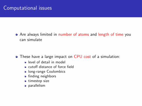
Computational issues

Are always limited in number of atoms and length of time youcan simulate

These have a large impact on CPU cost of a simulation:

level of detail in modelcutoff distance of force fieldlong-range Coulombicsfinding neighborstimestep sizeparallelism

Coarse-graining of polymer models

All-atom:

∆t = 0.5-1.0 fmsec for C-HC-C distance = 1.5 Angscutoff = 10 Angs

United-atom:

# of interactions is 9x less∆t = 1.0-2.0 fmsec for C-Ccutoff = 10 Angs20-30x savings over all-atom

Bead-Spring:

2-3 C per bead∆t ⇐⇒ fmsec mapping isT-dependent21/6σ cutoff ⇒ 8x in interactionscan be considerable savings overunited-atom

Cutoff in force field

Forces = 80% of CPU cost

Short-range forces:

O(N) scaling for classical MDconstant density assumptionpre-factor is cutoff-dependent

# of pairs/atom = cubic in cutoff

2x the cutoff ⇒ 8x the work

Use as short a cutoff as can justify:

LJ = 2.5σ (standard)all-atom and UA = 8-12 Angstromsbead-spring = 21/6σ (repulsive only)Coulombics = 12-20 Angstromssolid-state (metals) =few neighbor shellsdue to screening

Test sensitivity of your results to cutoff

Long-range Coulombics

Systems that need it:

charged polymers (polyelectrolytes)organic & biological moleculesionic solids, oxidesnot most metals (screening)

Computational issue:

Coulomb energy only falls off as 1/r

Options:

cutoff: scales as N, but large contribution at 10 AngsEwald: scales as N3/2

particle-mesh Ewald: scales as N log(N)multipole: scales as N, but doesn’t beat PMEmulti-level summation: scales as Ncan beat PME for low-accuracy, large proc count

PPPM (Particle-mesh Ewald)

Hockney & Eastwood, Comp Sim Using Particles (1988).

Darden, et al, J Chem Phys, 98, p 10089 (1993).

Like Ewald, except sum over periodic images evaluated:

interpolate atomic charge to 3d meshsolve Poisson’s equation on mesh (4 FFTs)interpolate E-fields back to atoms

User-specified accuracy + cutoff ⇒ ewald-G + mesh-size

Scales as N√

log(N) if grow cutoff with N

Scales as N log(N) if cutoff held fixed

Parallel FFTs (in LAMMPS)

3d FFT is 3 sets of 1d FFTs

in parallel, 3d grid is distributedacross procs1d FFTs on-processornative library or FFTW(www.fftw.org)multiple transposes of 3d griddata transfer can be costly

FFTs for PPPM can scale poorly

on large # of procs and on clusters

Good news: Cost of PPPM is only ∼2x more than 8-10 Ang cutoff

Neighbor lists

Problem: how to efficiently find neighbors within cutoff?

For each atom, test against all others

O(N2) algorithm

Verlet lists:

Verlet, Phys Rev, 159, p 98 (1967)Rneigh = Rforce + ∆skin

build list: once every few timestepsother timesteps: scan larger list for

neighbors within force cutoffrebuild: any atom moves 1/2 skin

Link-cells (bins):

Hockney et al, J Comp Phys,14, p 148 (1974)

grid domain: bins of size Rforce

each step: search 27 bins forneighbors (or 14 bins)

Neighbor lists (continued)

Verlet list is ∼6x savings over bins

Vsphere = 4/3 πr3

Vcube = 27 r3

Fastest methods do both

link-cell to build Verlet listuse Verlet list on non-build timestepsO(N) in CPU and memoryconstant-density assumptionthis is what LAMMPS implements

Timescale in classical MD

Timescale of simulation is most serious bottleneck in MD

Timestep size limited by atomic oscillations

C-H bond = 10 fmsec ⇒ 1/2 to 1 fmsec timestepDebye frequency = 1013 ⇒ 2 fmsec timestep

Reality is often on a much longer timescale

protein folding (msec to seconds)polymer entanglement (msec and up)glass relaxation (seconds to decades)rheological experiments (Hz to KHz)

Even smaller timestep for tight-binding or quantum-MD

Particle-time metric

Atom * steps = size of your simulation

Up to 1012 is desktop scale ⇒ 106 atoms for 106 timesteps

1 µsec/atom/step on CPU core (cheap LJ potential)2 weeks on single core, 1 day on multi-core desktop

1012 to 1014 is cluster scale

1014 and up is supercomputer scale

1 cubic micron (1010 atoms) for 1-2 nanoseconds (106 steps)

1000 flops per atom per step ⇒ 1019 flopsMD is 10% of peak ⇒ 1 day on a Petaflop machine

GPUs are changing landscape:can be 5-10x faster than multicore CPU

Extending timescale via SHAKE

Ryckaert, et al, J Comp Phys, 23, p 327 (1977)

Add constraint forces to freeze bond lengths & angles

rigid water (TIP3P)C-H bonds in polymer or protein

Extra work to enforce constraints:

solve matrix for each set ofnon-interacting constraints

matrix size = # of constraints

Allows for 2-3 fmsec timestep

Extending timescale via rRESPA

Tuckerman et al, J Chem Phys, 97, p 1990 (1992)

reversible REference System Propagator Algorithm

Rigorous multiple timestep method

time-reversibleoperator calculus ⇒

derivation of conserved ensemble quantities

Sub-cycle on fast degrees of freedom

innermost loop on bond forces (0.5 fmsec)next loop on 3-4 body forcesnext loop on van der Waals & short-range Coulombicoutermost loop on long-range Coulombic (4 fmsec)

Can yield 2-3x speed-up, less in parallel due to communication

Classical MD in parallel

MD is inherently parallel

forces on each atom can be computed simultaneouslyX and V can be updated simultaneously

Nearly all MD codes are parallelized

distributed-memory message-passing (MPI) between nodesMPI or threads (OpenMP, GPU) within node

MPI = message-passing interface

MPICH or OpenMPIassembly-language of parallel computinglowest-common denominatormost portableruns on all parallel machines, even on multi- and many-coremore scalable than shared-memory parallel

Goals for parallel algorithms

Scalable

short-range MD scales as Noptimal parallel scaling is N/Peven on clusters with higher communication costs

Good for short-range forces

80% of CPUlong-range Coulombics have short-range component

Fast for small systems, not just large

nano, polymer, bio systems require long timescales1M steps of 10K atoms is more useful than 10K steps of 1Matoms

Efficient at finding neighbors

liquid state, polymer melts, small-molecule diffusionneighbors change rapidlyatoms on a fixed lattice is simpler to parallelize

Parallel algorithms for MD

Plimpton, J Comp Phys, 117, p 1 (1995)

3 classes of algorithms used by all MD codes1 atom-decomposition = split and replicate atoms2 force-decomposition = partition forces3 spatial-decomposition = geometric split of simulation box

All 3 methods balance computation optimally as N/P

Differ in key issues for parallel scalability

communication costsload-balance

Focus on inter-particle force computation,other tasks can be done within any of 3 algorithms

molecular forcestime integration (NVE/NVT/NPT)thermodynamics, diagnostics, ...

Spatial-decomposition algorithm

Physical domain divided into 3d boxes,one (or more) per processor

Each proc computes forces on atomsin its box using ghost infofrom nearby processors

Atoms carry along molecular topologyas they migrate to new procs

Communication via 6-way stencil

Advantages

communication scales sub-linear as(N/P)2/3, for large problems

memory is optimal N/P

Disadvantages

more complex to code efficientlyload-imbalance can be problematic

Freely available parallel MD codes

Bio-oriented MD codes

CHARMM: original protein force fieldsAMBER: original DNA force fieldsNAMD: fast and scalableGromacs: fastest and scalable

Materials-oriented MD codes (can also do bio problems):

DL POLY: distributed by Daresbury Lab, UKLAMMPS: distributed by Sandia National Labs

GPU-centric MD code (materials and bio):

HOOMD: distributed by U Michigancodes above have GPU-capable kernels

What is LAMMPS?

Large-scale Atomic/Molecular Massively Parallel Simulatorhttp://lammps.sandia.gov

Classical MD code

Open source (GPL), highly portable C++

3-legged stool: bio, materials, mesoscale

Particle simulator at varying length and time scaleselectrons ⇒ atomistic ⇒ coarse-grained ⇒ continuum

Spatial-decomposition of simulation domain for parallelism

Energy minimization, dynamics, non-equilibrium MD

GPU and OpenMP enhanced

Can be coupled to other scales: QM, kMC, FE, CFD, ...

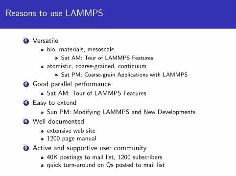
Reasons to use LAMMPS

1 Versatilebio, materials, mesoscale

Sat AM: Tour of LAMMPS Features

atomistic, coarse-grained, continuum

Sat PM: Coarse-grain Applications with LAMMPS

2 Good parallel performance

Sat AM: Tour of LAMMPS Features

3 Easy to extend

Sun PM: Modifying LAMMPS and New Developments

4 Well documented

extensive web site1200 page manual

5 Active and supportive user community

40K postings to mail list, 1200 subscribersquick turn-around on Qs posted to mail list

Another reason to use LAMMPS

6 Features for rheology (next 2 days)

Mesoscale models:DPD = dissipative particle dynamicsSPH = smoothed particle hydrodynamicsgranular = normal & tangential frictionFLD = fast lubrication dynamicsPD = peridynamicsrigid body dynamics

Aspherical particlespoint ellipsoidsrigid body collections of points, spheriods, ellipsoidsrigid bodies of triangles (3d) and lines (2d)

Coarse-grained solvent modelsrigid waterpolymers (united-atom, bead-spring)LJ particlesstochastic rotation dynamics (SRD)implicit

More rheological options in LAMMPS

Many of these options came from 4-year collaborationwith 3M, BASF, Corning, P&G on solvated colloidal modeling

Particle/particle interactions:pair gayberne, resquared, colloid, yukawa/colloid, vincentpair brownian, lubricate, lubricateU (implicit)pair gran/hooke and gran/hertzpair hybrid/overlay for DLVO modelsfix srd for colloids + SRD fluid

Packages:ASPHERE, COLLOID, FLD, GRANULARRIGID, SRD, USER-LB

2 methods for measuring diffusivitymean-squared displacement via compute msdVACF via post-processing of dump file

3 methods for measuring shear (or bulk) viscositiesNEMD via fix deform and fix nvt/sllod or fix wallMuller-Plathe via fix viscosityGreen-Kubo via fix ave/correlate

Examples of rheological simulations

Polymer aggregation under shear

More examples of rheological simulations

Diffusion and viscosity of solvated dimers

Still more examples of rheological simulations

Viscosity of asphericals in SRD fluid

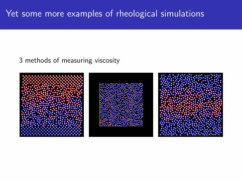
Yet some more examples of rheological simulations

3 methods of measuring viscosity

Finally, enough of rheological simulations

Arbitrary-shape asphericals via lines and triangles

See http://lammps.sandia.gov/movies.html to view all theseanimations and for links to input scripts