(How) Do Taxes Affect Capital Structure? - Wharton Faculty · PDF file(How) Do Taxes Affect...
52
(How) Do Taxes Affect Capital Structure? ∗ Andrew MacKinlay † January 2012 Abstract I find the effect of taxes on firms’ overall debt usage to be insignificant. Rather than influencing the total debt in firms’ capital structure, taxes affect the relative composition of debt. Firms shift from private intermediated debt to public bond debt in response to increases in marginal tax rates. Firms’ debt policy is most sensitive to tax rates in high interest rate environments. In policy experiments, I find that proposed tax law changes would likely have little effect on debt usage. ∗ I am indebted to my dissertation committee, Michael Roberts (Chair), Itay Goldstein, Mark Jenkins, and Krishna Ramaswamy for many helpful discussions and guidance. I also thank Andy Abel, Jennifer Blouin, Vincent Glode, Todd Gormley, David Musto, Greg Nini, Christian Opp, Nick Roussanov, Ivan Shaliastovich, Nicholas Souleles, and Luke Taylor for their comments. Financial support from the Robert R. Nathan Fellowship is gratefully acknowledged. † The Wharton School, University of Pennsylvania, 2300 Steinberg-Dietrich Hall, 3620 Locust Walk, Philadel- phia, PA 19104. Email: [email protected]. Phone: (610) 304-8756.
Transcript of (How) Do Taxes Affect Capital Structure? - Wharton Faculty · PDF file(How) Do Taxes Affect...

(How) Do Taxes Affect Capital Structure?∗
Andrew MacKinlay†
January 2012
Abstract
I find the effect of taxes on firms’ overall debt usage to be insignificant. Rather thaninfluencing the total debt in firms’ capital structure, taxes affect the relative compositionof debt. Firms shift from private intermediated debt to public bond debt in response toincreases in marginal tax rates. Firms’ debt policy is most sensitive to tax rates in highinterest rate environments. In policy experiments, I find that proposed tax law changeswould likely have little effect on debt usage.
∗I am indebted to my dissertation committee, Michael Roberts (Chair), Itay Goldstein, Mark Jenkins, andKrishna Ramaswamy for many helpful discussions and guidance. I also thank Andy Abel, Jennifer Blouin,Vincent Glode, Todd Gormley, David Musto, Greg Nini, Christian Opp, Nick Roussanov, Ivan Shaliastovich,Nicholas Souleles, and Luke Taylor for their comments. Financial support from the Robert R. Nathan Fellowshipis gratefully acknowledged.
†The Wharton School, University of Pennsylvania, 2300 Steinberg-Dietrich Hall, 3620 Locust Walk, Philadel-phia, PA 19104. Email: [email protected]. Phone: (610) 304-8756.

United States tax law provides firms with an incentive to issue debt. The extent to which
firms react to this incentive is unclear. Fama and French (1998) are unable to find evidence
of a positive relation between leverage and firm value. In contrast, Graham (2000) estimates
that the tax benefits of debt are large and that the typical firm could add considerably to its
value by increasing its leverage ratio. In survey evidence, Graham and Harvey (2001) find that
CFOs consider interest tax savings to be moderately important for debt policy, ranking behind
financial flexibility and cash flow volatility concerns, but ahead of transaction costs and distress
costs. Reviewing the evidence, Myers concludes that although there are examples of specific
tax-driven financing tactics such as financial leases, “finding clear evidence that taxes have a
systematic effect on financing strategy, as reflected in actual or target debt ratios, is much more
difficult.” (Myers, 2003, p. 225).
This paper contributes to the debate by evaluating the role of taxes in firms’ debt and equity
issuance decisions. Specifically, I estimate firm-specific demand curves for debt capital. These
curves capture the probability that a firm will issue debt as a function of its cost, its tax rate,
and other relevant firm characteristics. Unconditionally, I find no relation between marginal
tax rates and debt issuance.1 This result holds not only for how likely a firm is to issue debt,
but also when the quantity of debt issued is considered.
Although the overall demand for debt is insensitive to marginal tax rates, marginal tax rates
do affect the composition of a firm’s debt. Recognizing that debt is heterogeneous and debt
structure is an important element of capital structure (Rauh and Sufi, 2010), I separate debt
into two major types: privately raised bank debt and publicly issued bond debt. As marginal
tax rates increase, firms substitute away from private bank debt and into public bond debt. An
increase in firms’ marginal tax rates alters the relative after-tax costs of the two debt types and
makes the more expensive but less restrictive public debt more desirable.
Conditionally, the effect of taxes on capital structure is strongest in high interest rate envi-
ronments. Differences in taxes matter when the value of interest tax shields is potentially large.
1The marginal tax rate is defined as the present value of current and futures taxes paid on an additional dollarof current period income.
1

In these environments, the largest shifts between public and private debt occur and high-tax
firms are more likely to issue debt. In periods with low costs of debt, there is little observed
difference in the issuance behavior of firms attributable to taxes.
The incentive to operate with high leverage because of the tax deductibility of interest paid
on debt is a popular policy issue. Some policymakers advocate lowering the corporate tax rate
to induce firms to take on less debt. They argue that these lower debt levels would reduce
firms’ risk of bankruptcy and aggregate risk in the economy. Using my demand estimates,
I investigate the impact of such a hypothetical corporate tax cut on firm financing choices.
Consistent with the results discussed above, altering the corporate tax rate does not change
firms’ overall propensity to issue debt. Instead, firms move from public bond debt to private
bank debt, and this move is most pronounced in market environments when the cost of debt is
highest. Because firms raise similar quantities of debt in the public and private debt markets,
the substitution would not translate into lower leverage ratios. Although there may be other
reasons for corporate tax reform, the leverage channel does not appear to be important.
Several empirical studies have found a significant positive relation between firms’ marginal
tax rates and debt usage.2 My paper recognizes that observed capital structures are the product
of firms’ demand for financial capital and capital markets’ willingness to supply this capital.
Recent research provides evidence that the condition of lenders affect the price and quantity
of capital available to firms.3 To the extent that supply shocks occur in specific debt markets,
such as bank loans or public bonds, the relative cost and availability of these different types of
debt change as well.
In equilibrium, the cost of debt is simultaneously determined by firms’ demand for capital
and the supply conditions of banks and other capital providers. Because the cost is correlated
with other relevant firm characteristics, not all of which are observable, a naı̈ve estimation finds
that firms are not sensitive to the cost of debt. To address this endogeneity and properly identify
2See MacKie-Mason (1990), Graham (1996a), and Graham, Lemmon, and Schallheim (1998).3These papers include Faulkender and Petersen (2006), Sufi (2009), Leary (2009), Lemmon and Roberts
(2010), and Chava and Purnanandam (2011).
2

the role of the cost of debt capital, I use exogeneous variation in the capital supply of banks
and insurance companies. This supply variation, provided by unrelated bank loan losses and
insurance losses, allows me to isolate firms’ demand curves for both private and public debt
from the observed issuance decisions.
When properly identified, firms’ demand for debt is strongly decreasing in its cost. Firms
with higher marginal tax rates are more profitable, less risky, and therefore face a lower pre-tax
cost of debt. In traditional regressions of financial policy measures on proxies for the marginal
tax rate, these two sources of variation—tax incentives and cost differences driven by future
profitability—are commingled. Separating the two sources of variation, the effect of taxes on
overall debt usage is minimal. Although many theoretical studies use taxes as the key debt
policy determinant, this result suggests alternative mechanisms may be of higher importance.
Although the focus of this paper is on the role of taxes in capital structure, the framework
used here is not limited to that question. Isolating firms’ demand curves for debt from ob-
served capital structure is important for understanding the role of any potential friction to the
debt decision. These demand curves show whether commonly cited frictions—such as distress
costs, agency conflicts, and information asymmetries—are actively considered by firms, or if
the observed data that is consistent with these frictions is an artifact of changes in the supply of
capital. When frictions do affect firm demand, the shift in demand curves resulting from these
frictions quantifies their relative importance.
The remainder of the paper is structured as follows. Section 1 describes the empirical
hypotheses. Section 2 presents the empirical model. Section 3 discusses the data used for this
study. Section 4 discusses the endogeneity and instrumentation of the cost of debt. Section 5
presents the results. Section 6 presents the policy implications, and Section 7 concludes.
3

1 Empirical Hypotheses
Because this paper explicitly incorporates both the pre-tax cost of debt and multiple types of
debt, I first present a stylized model to illustrate the main effects at work for taxes and the
pre-tax cost of debt. In the main empirical specification in Section 2, the model is generalized
to allow for additional factors that affect debt policy. The stylized model is a simple linear
demand equation:
DD(τC , rD) = α− β(1− τC)rD, (1)
where the firm’s demand for debt is a function of its marginal tax rate, τC , and its pre-tax
cost of debt, rD. Demand factors unrelated to taxes and the cost of debt are represented by the
coefficient α. The firm’s demand is decreasing in the after-tax cost of debt, β(1−τC)rD, where
β > 0.
Equation (1) abstracts from many other factors that feed into the firm’s debt decision. The
purpose of this simpler demand function is to develop hypotheses for how tax rates and the pre-
tax cost of debt affect the firm’s demand for debt; these factors are included in the estimated
generalized demand function. Considering the pre-tax cost of debt in equation (1), it follows
that holding all else equal, a firm’s demand for debt capital is decreasing in its cost.
Hypothesis 1: Firms with a higher pre-tax cost of debt capital are less likely to issue debt,
∂DD(τC , rD)
∂rD= −β(1− τC) < 0. (2)
For example, if the pre-tax cost of private debt increases, firms should move to other types of
capital or refrain from raising external capital altogether.
Because interest payments are tax-deductible, a firm with a higher taxable income benefits
from debt financing. For a firm with no taxable income or already fully shielded income, the
tax shields associated with new debt are not usable and therefore not valuable. In equation (1),
this benefit is captured by (1− τC), where τC varies from the top statutory rate for a firm with
4

substantial taxable income to near zero for a firm with little or no taxable income.
Hypothesis 2: Firms facing a higher tax rate demand debt more than firms facing a lower tax
rate,∂DD(τC , rD)
∂τC= βrD > 0. (3)
Another implication of equation (1) is that differences in τC among firms lead to hetero-
geneity in the reaction to changes in the pre-tax cost of debt capital, rD. Specifically, for firms
with higher tax rates, a given change in the pre-tax cost of debt has a more muted effect on the
demand for debt.
Hypothesis 3: Firms with a higher tax rate are less sensitive to changes in the pre-tax cost of
debt capital than firms with a lower tax rate,
∂2DD(τC , rD)
∂rD∂τC= β > 0. (4)
Because ∂DD(τC , rD)/∂rD < 0, the positive derivative in equation (4) means that ∂DD(τC , rD)/∂rD
is negative but with smaller magnitude the higher τC . Hypothesis 3 concerns a tax effect on the
elasticity, as opposed to the level, of demand for debt. When the pre-tax cost of debt is omitted
from the estimation, this effect is ignored.
These implications apply to a firm focusing on a single debt option. A firm’s demand
for debt is different when there are multiple debt types. With different debt types, the linear
demand equation can be expanded:
DD1(τC , rD1, rD2) = α− β(1− τC)rD1 + γ(1− τC)rD2. (5)
In this equation, debt is one of two types (D1, D2), and the cost of the other type of debt is
directly incorporated into the demand equation. If γ > 0, an increase in the cost of the other
debt type makes the current option more desirable. Assuming rD1 represents the pre-tax cost
of private debt, the firm’s demand for private debt is now a function of its own cost and the
5

pre-tax cost of public debt, rD2. A change in tax rate now has two effects:
∂DD1(τC , rD1, rD2)
∂τC= βrD1 − γrD2. (6)
The first term in the derivative is the same effect as stipulated in Hypothesis 2. With multiple
debt types, there is a countervailing effect, −γrD2. This second term captures the extent to
which the firm substitutes to the other debt type as tax rates change. Because tax rates affect
demand for debt through the cost of debt, the levels of rD1 and rD2 determine how a firm reacts
to a tax-rate change. The relative magnitudes of the two terms in equation (6) could lead the
firm to demand less of a type of debt as its marginal tax rate increases.
2 Empirical Model
The hypotheses in Section 1 are empirically testable. The firm’s demand for debt, DD, is typi-
cally specified in one of three ways. The most common approach is to use the firm’s leverage
ratio (Rajan and Zingales, 1995; Graham et al., 1998; Rauh and Sufi, 2010). Alternatively,
one can consider changes in the quantity of debt issued (Graham, 1996a). The third alterna-
tive is to focus on discrete debt issuances and consider the probability of a firm issuing debt
(MacKie-Mason, 1990; Gomes and Phillips, 2005).
Because each debt decision has two components—the quantity of debt chosen and the type
of debt chosen—none of these alternatives fully captures the firm’s demand for debt. Using
leverage ratios or changes in total debt ignores the type of debt issued. Even if one considers
the quantity of debt or leverage ratio for a specific type of debt, as in Rauh and Sufi (2010), the
explicit choice of the type of debt is not modeled. Considering the discrete issuance decisions
of firms, the quantity choice is necessarily de-emphasized.
To consider the role of taxes when the firm chooses between types of debt with different
characteristics, this paper focuses on the discrete issuance decision. As equation (5) suggests,
debt types with different costs and characteristics imply additional tax effects. These additional
6

effects are ignored when debt is treated as a single entity. Looking at discrete issuance decisions
allows measurement of these additional effects. If these additional effects are significant, how
a firm substitutes across different types of debt is an important consideration for understanding
observed capital structure and the impact of potential tax policy changes.
The importance of the type of debt does not make the quantity of debt an irrelevant concern.
Although not the central focus, Section 5.5 considers the empirical hypotheses in terms of the
quantity of debt chosen. Section 5.5 also discusses how firms’ quantity decisions may affect
inferences about firms’ debt-type decisions.
Because I test how a firm’s issuance decision depends on both characteristics of the firm
(particularly its marginal tax rate) and the pre-tax cost of different types of debt, I use a condi-
tional logit framework. This model is well-developed in the economics literature, going back
to McFadden (1974). Each firm has three security choices—public debt, private debt, and
equity—and can opt not to raise external capital.4
The key assumption of the model is that for the set of possible security issuance choices,
including foregoing issuance, the firm chooses the option in its best interest. The value to firm
i of issuing security j in calendar year-quarter t is captured by the latent variable vijt. Because
vijt is not directly observable, it is inferred from the observed decisions of firms over time.
Given that only relative preferences are revealed by observed firm decisions, the absolute level
of vijt is not identified. To address this issue, I normalize by assuming vijt = 0 for the option
of not issuing any security. A choice with a value of vijt > 0 denotes the security issuance
is more favorable than the option of not issuing, and a value of vijt < 0 denotes the security
issuance is less favorable than not issuing.
4Allowing firms the outside option of choosing not to issue a security is important for a few reasons. First,although the firms I consider have all raised external capital, they do not do so regularly. Specifying the model asbeing conditional on a firm issuing a security would ignore the dynamics that compel a firm to raise capital in thefirst place. Without including this option, for any changes in firm or security characteristics, the model assumesthe firm would still raise capital. It is plausible, however, that a firm may delay or decide not to raise capital ifthe cost of the security or the firm itself undergoes a material change. Using a model which includes the outsideoption does not impose this restriction.
7

For purposes of estimation, vijt is characterized as follows:
vijt = β0,j + β1rijt + β2,jτit + β3,jτit · rijt + β ′4,jft + β ′
5,jmt︸ ︷︷ ︸voijt
+εijt. (7)
The variable vijt is a function of observables, voijt, and an unobserved error term, εijt. The
observable part voijt is composed of a security-specific constant β0,j , the pre-tax cost of debt or
equity capital, rijt, the firm’s marginal tax rate, τit, other firm characteristics fit, and macro-
economic variables mt. The error term, εijt, captures any unobserved or unspecified drivers of
demand. Because certain variables, such as firm characteristics and macroeconomic variables,
do not vary over security choices for a specific firm in a specific quarter, their impact is captured
by permitting the coefficients to vary by security type j. As such, a positive coefficient denotes
that an increase in the related variable increases the demand for that security, relative to the
outside option. The cost of the outside option is set to zero.
Equation (7) is a generalization of the simple linear demand given by equation (1). The firm
characteristics, macroeconomic variables, and the security-specific constant in equation (7) are
included to control for the non-tax and non-cost determinants of the firm’s demand for a specific
type of capital. In equation (1), these elements are included in α. One additional generalization
is the inclusion of τit separate from rijt. This term allows for the possibility that the firm’s
marginal tax rate affects the firm’s decision beyond its effect on the cost of debt. If taxes play a
role only through adjusting the cost of debt, as equation (1) assumes, the coefficient β2,j should
be zero.
Although equation (7) has been the focus of discussion until this point, the conditional logit
estimation gives the firm’s demand as the probability of issuing that security. The probability
of issuance, Pijt, is defined as:
Pijt = Prob(voijt + εijt > voikt + εikt, ∀k �= j). (8)
8

The value of Pijt depends not only on the latent value of security j, vijt, but also on the latent
value of all the other security choices for firm i in quarter t. In other words, the probability of
a firm issuing public debt depends not only on the cost of public debt and whether the firm’s
characteristics make public debt desirable, but also on the cost of private debt and whether
the firm’s characteristics make private debt desirable. Because the model is structured in this
manner, it captures not only how changes in the pre-tax cost of public debt affect the demand for
public debt, but also how changes in the pre-tax cost of private debt affect the demand for public
debt. Therefore the model captures the cross-elasticities that are modeled in equation (5).
The model can be estimated using standard conditional logit estimation techniques but for
two complications. First, there is a missing data issue. The pre-tax costs of public and private
debt for firms are only observed when one of these types is chosen. Imputing the missing pre-
tax cost of debt data is discussed in Section 3.3. Second, the pre-tax cost of debt is endogenous
to the firm’s demand for debt. This endogeneity issue and the instrumental variables approach
used to resolve it are discussed in detail in Section 4.
3 Data and Summary Statistics
The sample of firms chosen is restricted to nonfinancial firms that are in the Compustat universe
and have a Standard and Poor’s credit rating between A+ and B-. The sample of firms are
constructed this way for two reasons. First, focusing on firms with a public debt rating assures
that the different securities choices—private debt, public debt, and equity—are all feasible for
the firms considered. Second, a firm’s credit rating aids in estimating the cost of the different
securities. This results in 1,644 unique nonfinancial firms from the first quarter of 1988 through
the first quarter of 2010.
9

3.1 Issuance Data
Data on firms’ issuance decisions comes from three sources. For the private debt market,
I use the DealScan database, which covers both single-lender and syndicated multiple-lender
loans. For the public debt market, I use the Mergent FISD database for origination information.
For equity issuance, I track issuances using quarterly split-adjusted share growth data from
CRSP: in order to restrict equity issuances to those that are related to raising capital and not for
executive compensation, I require the amount raised to be at least 3% of the previous quarter’s
book assets.
For modeling purposes, I assume a firm can only raise one type of capital in a given calendar
year-quarter. When a firm issues multiple securities in the same calendar year-quarter, I use the
following procedure. The issues are aggregated to provide the total amount of capital raised in
that quarter, and then classified under the type that the majority of the capital is raised under. If
the majority is a debt issuance, the maturity and yield are determined from a value-weighting
of the individual issues. In practice, most firms do not issue across the security types used
here. In the final sample, only 451 firm-quarters issued both equity and debt simultaneously,
and only 646 issued both private and public debt. Given the 29,487 total firm-quarters in the
final sample, multiple issuances that cross security types account for only 3.5% of the sample.
Table 1 details how firms raise capital in the sample period: on average, 79.3% of firms do
not raise capital, 9% of firms issue private debt, 8.1% of firms issue public debt, and 3.6% of
firms issue equity in a given quarter. The average yield to maturity that a firm pays to raise
debt is 5.87% for private debt and 7.24% for public debt. Private debt tends to be shorter term
in maturity, with an average maturity of 4.2 years compared to 12.5 years for public debt.
The amount of capital raised varies across types. Public debt issuances raise $388 million
on average, whereas private debt raises $859 million. Private debt amounts are the total capital
that can be drawn from the issuance, and not necessarily the actual amount drawn. This dis-
tinction may partly explain why private debt has higher capital amounts.5 The average equity
5About 25% of private debt issuances included a revolving credit line. The average capital raised for private
10

issuance is substantial at $729 million, and that average is the result of substantial skew; the
median equity issuance being much smaller at $135 million. This amount compares to median
values of $250 million for public debt and $394 million for private debt. Although there are a
few enormous equity issuances in the sample, the majority are smaller than for other types of
external capital.
3.2 Firm Characteristics and Macroeconomic Variables
Table 1 also includes the firm characteristics that are used in the demand estimation. All firm
characteristics are from the quarter prior to the issuance decision. The exceptions are the sim-
ulated marginal tax rate and statutory tax rate variables, which are from the most recent fiscal
year prior to the current calendar quarter. Because the focus is on the tax incentives of security
issuance, proxied for by the marginal or statutory tax rate variable, the other variables are in-
cluded as controls for the elements of security demand that are unrelated to tax considerations.
The Marginal Tax Rate (MTR) variable is from John Graham’s website. A firm’s future
income is simulated using a constrained random walk process; the expected present value of
additional current and future taxes from one extra dollar of current-period income is deter-
mined by averaging over these simulations.6 The Statutory Tax Rate variable is defined as the
current U.S. federal statutory tax rate given the firm’s taxable income minus any tax loss carry
forwards.
The Market-to-Book ratio is included to capture differences in investment opportunities of
firms. Asset tangibility (Tangibility), defined as the ratio of fixed assets (property, plants, and
equipment) to total book assets, is included to capture differences in collateral among firms.
Because firms with higher marginal tax rates may have higher current and future profitability, I
include three additional variables. Profitability is simply last quarter’s operating income scaled
debt issuances without a credit line is $675 million.6Graham (1996b) argues the simulated tax rates are the best available proxy for marginal tax rates. More
details as to the variable’s construction can also be found in Graham and Mills (2008). See Blouin, Core, andGuay (2010) for an alternative method of simulating future income for the purposes of calculating marginal taxrates.
11

by book assets. Profitability Drift is the average quarterly change in the firm’s operating income
scaled by last quarter’s book assets.7 Profitability Volatility is calculated similarly, but is the
volatility of quarterly operating income scaled by last quarter’s book assets. These drift and
volatility variables are used to control for differences in the future profitability of the firm.
Earnings Yield, the cost-of-equity variable, is calculated with firm-specific earnings fore-
casts from the IBES database.8 The quarterly stock return (Stock Return) is included as an ad-
ditional control for changes in equity valuation, and the Earnings Surprise variable is a proxy
for information asymmetry. Altman’s Z-Score captures differences in the financial condition of
firms.9
In considering incremental debt and equity issuances by firms, the model should account
for the existing capital structure. I include the existing total leverage ratio (Leverage) of firms,
the ratio of short-term debt to assets (Short-Term Debt to Assets), and the ratio of cash to assets
(Cash to Assets). These variables capture the extent of pre-existing leverage, how much debt is
due in the coming year, and how much cash is on hand to absorb any financing needs.
When firms do use the external markets, they raise substantial amounts of capital. The
average capital raised as a percent of the previous quarter’s book assets ranges from 13% for
equity and public debt to 19% for private debt. In order to capture differences in the need for
funds among firms, I include a Financing Need variable. This variable is the sum of the internal
funding deficit of a firm over the past four quarters prior to the current calendar quarter, scaled
by the previous quarter’s book assets.
Beyond issuance and firm accounting variables, some additional macroeconomic and supply-
side variables are used as controls in the analysis. United States government debt yield data and
other U.S. macroeconomic data comes from the St. Louis Federal Reserve (FRED) database.
Quarterly year-over-year GDP growth (GDP Growth) is included to capture the effect of larger
7This average operating income change is computed on a rolling basis, requiring a minimum window of fiveyears. Results are unchanged if the estimation window is restricted to five years.
8Specifically, earnings yield is the median forecast of earnings for the next four quarters divided by the shareprice as of the end of the last calendar quarter.
9See Appendix A for additional details about variable construction.
12

business-cycle variation on security-issuance decisions; the CRSP value-weighted stock return
index (CRSP VW Market Return) captures aggregate stock market movements. The three-
month treasury bill rate (3-Month T-Bill) is also included to capture changes in interest rates
driven by U.S. monetary policy. Like the firm variables, these macroeconomic variables are
from the prior quarter in the estimation.
3.3 Cost of Debt and Equity
In the framework used here, the cost of public debt, private debt, and equity are needed for
every firm-quarter to estimate equation (7). When the firm issues public or private debt, the
yield to maturity is a clear measure of the pre-tax cost. Establishing the pre-tax cost if the firm
did not issue debt, however, poses a problem. To address this missing data, the pre-tax cost of
debt for public and private debt are imputed from the observed issuances of firms that did raise
debt. Specifically, I assume that the pre-tax cost of debt for a firm in a given quarter is the same
as what other firms of similar credit risk pay, adjusting for observable firm characteristics that
affect the pre-tax cost of debt. This assumption provides a means to estimate the pre-tax cost
of debt for securities not chosen:
rijt = γ0 + γ′1fit + γ′
21cr + γ′31t + εijt, (9)
where the pre-tax cost of debt for security j for firm i in year-quarter t is a function of firm
characteristics, fit, as well as credit rating (cr) and year-quarter fixed effects. I estimate equa-
tion (9) separately for private and public debt and use the estimated coefficients to generate the
yields on each security for each firm-quarter. The coefficients for this estimation are presented
in Table 2.10
One issue is that if debt is risky, the yield is not the same as the cost of debt (Berk and
10An alternate specification, in which credit rating by year-quarter fixed effects are used instead of separatecredit rating and year-quarter fixed effects, generates very similar results. The main specification has the advantagethat for quarters in which very few securities are issued in a specific credit rating, the average yield captured bythe fixed effects is far less noisy.
13

DeMarzo, 2009). As a final step, these imputed yields, denoted r̂ijt, are adjusted by the firm’s
probability of default and the security type’s expected loss, given default. The probability of
default is specific to the credit rating of the firm, and the loss rate is dependent on whether the
security is a bank loan (the assumption for private debt) or an unsecured senior bond (the as-
sumption for public debt).11 This adjustment makes the imputed yields a better approximation
of the pre-tax cost of debt capital for the firm.
The pre-tax cost of debt for a firm also depends on the specifics of the particular debt
contract, such as the quantity of capital raised, the maturity of the contract, and any additional
contract provisions that make the debt more or less risky. The nuances of specific contracts
cannot be captured in the imputation done in equation (9). The imputed cost of debt should be
considered as the yield associated with the average public or private debt issuance for firms with
similar characteristics at that time. Differences in debt contracts that arise from differences in
the credit quality and other characteristics of firms are captured in equation (9); the associated
differences in yield are reflected in the imputation. To avoid comparing the actual yield for a
chosen debt type, which reflects very specific contract terms, against the imputed yield for the
other debt type, which is the average or typical yield for that type of firm, only the imputed
yields are used in the estimation model.
A forecast-based earnings yield is used as a proxy for the cost of equity. Because the
earnings yield is available every quarter for firms in the sample, an imputation step is not
necessary.
11Default probabilities and loss rates are calculated using Moody’s annual corporate default and recovery ratedata. Specifically, the default rate is determined as an annualized rate for defaults in each credit rating over thepast ten years, calculated on a rolling basis. The expected loss on the security is taken to be 19.9% for private debtand 55.4% for public debt.
14

4 Identification Strategy
4.1 The Identification Problem
Estimating the effect of the pre-tax cost of debt in equation (7) is susceptible to three potential
sources of endogeneity: a simultaneity bias, correlation with omitted security characteristics,
and measurement error. Because the pre-tax cost is determined simultaneously by firm demand
and capital supply, changes in the firm’s demand for debt directly affect the cost at which the
debt is available. In this case, increases in aggregate firm demand for debt increase the cost
of debt, and thus the estimate of the effect of the pre-tax cost of debt in equation (7) is biased
upward.
The firm’s demand for a particular security is affected by omitted security characteristics
that are correlated with the security’s cost. Because the costs are imputed using time-fixed
effects and firm characteristics, idiosyncratic omitted characteristics are not an issue. While
these omitted characteristics are in the error term, they are not correlated with the imputed cost.
Insofar as specific securities may undergo trends in characteristics at an aggregate level, these
omitted characteristics remain correlated with the imputed costs. This type of endogeneity also
biases the coefficient on the cost of debt in equation (7) upward.
Although the imputation step breaks the correlation between cost of debt and idiosyncratic
omitted characteristics, the difference between the imputed cost of debt and true cost of debt
is measurement error. When this measurement error is uncorrelated with the imputed cost, it
is not problematic. If, instead, the classical errors-in-variables assumption holds that the true
cost of debt and measurement error are uncorrelated, then the estimate of the coefficient for
the cost of debt in equation (7) is attenuated toward zero. The remaining coefficients are also
potentially biased depending on their correlation with the cost of debt.12
All three of these sources of endogeneity bias the coefficient for the cost of debt towards
zero. For the simultaneity and omitted variable biases, the bias can lead to a positive coefficient
12For a more detailed discussion of the endogeneity issues associated with measurement error, simultaneityissues, and omitted variables, see Roberts and Whited (2011).
15

for the cost of debt in equation (7). In these extreme cases, the estimation implies that a firm
prefers to pay more for debt capital, all else held equal. To identify the true effect of the cost of
debt on the firm’s demand for debt, I use an instrumental variables approach described below.
4.2 Control Function Approach
Focusing on the firm’s demand for debt, the impact of these sources of endogeneity is best
explained as an omitted variables bias. The unobserved error in equation (7) can be sepa-
rated into two independent parts: εijt = ε(1)ijt + ε
(2)ijt . Let ε(1)ijt be the demand shocks correlated
with the imputed cost of debt, r̂ijt. The true idiosyncratic preference shocks are captured by
ε(2)ijt . This component contains any shocks not correlated with the observable variables, in-
cluding the pre-tax cost of debt; by assumption it follows a type I extreme value distribution.
This error assumption produces the traditional logit framework used in discrete choice models.
The remaining error, ε(1)ijt , captures the simultaneity, omitted variable, and measurement error
problems that bias the estimation. The correlation between this error and the cost of debt is
addressed using instruments.
In a linear framework, instruments are applied using a two-stage least squares approach. In
the first stage, the imputed cost is regressed on the instruments and observed demand charac-
teristics:
r̂ijt = α′0zijt + α′
1,jfit + α′2,jmt + μijt, (10)
in which zijt are the instruments. Any potential instrument needs to satisfy two requirements:
(1) it must affect the cost of debt (relevance), and (2) it must not factor into the firm’s demand
for a security (exclusion). Specifically, the instruments provide variation in the imputed yields
that are not correlated with the problematic error, ε(1)ijt . Therefore, in equation (10), only μijt is
correlated with ε(1)ijt . The fitted values from equation (10) are by construction uncorrelated with
μijt, and hence ε(1)ijt . Replacing the original imputed cost with the fitted values corrects for the
omitted variables bias in equation (7).
16

In the non-linear framework used here, there is an analogous approach which requires
slightly more structure. Under the assumption that μijt and ε(1)ijt are not only correlated but
are jointly normally distributed, estimates of μijt resolve the omitted variables bias. Intuitively,
instead using fitted values of r̂ijt from equation (10) and thus eliminating the correlation with
ε(1)ijt , the correlation is maintained but ε(1)ijt is made observable. Once the problematic error is
observable, the correlation is no longer a source of bias.
This methodology is referred to as the control function approach (Heckman and Robb,
1985; Rivers and Vuong, 1988; Petrin and Train, 2010). Since μijt and ε(1)ijt are assumed jointly
normally distributed, ε(1)ijt is a function of the estimates of the residuals μijt from equation (10):
CF (ε(1)ijt) = βμ̂ijt + σηijt. (11)
Here β is the coefficient from the linear projection of ε(1)ijt on μijt, and ηijt is a standard normal
variable.13 This control function replaces ε(1)ijt in the main estimation equation:
vijt = β0,j + β1r̂ijt + β2,jτit + β3,jτit · r̂ijt + β ′4,jft + β ′
5,jmt + β6μ̂ijt + σηijt + ε(2)ijt . (12)
Because the part of ε(1)ijt that was correlated with r̂ijt is observable through β6μ̂ijt, equation (12)
can be estimated without β1 being biased.14
After including imputed costs and the control function, the final form of vijt is equation
(12). The probability of issuance derived from equation (12) is a mixed conditional logit be-
cause the error distribution is a mixture of a type I extreme value variable, ε(2)ijt , and a normal
13Specifically, under the assumption of uijt and ε(1)ijt being jointly normally distributed, the coefficient is given
by: β =ρσ
ε(1)
σu.
14The control function corrects the bias on β3,j as well. This aspect contrasts with the two-stage least squaresapproach, in which each interaction term is separately instrumented and replaced with fitted values. See Imbensand Wooldridge (2007) for more details.
17

variable, ηijt. The probability of issuance is defined as:
Pijt =1
N
N∑n=1
exp(β0,j + β1r̂ijt + β2,jτit + β3,jτit · r̂ijt + β ′
4,jfit + β ′5,jmt + β6μ̂ijt + σηn,ijt
)∑J
k=0 exp(β0,k + β1r̂ikt + β2,kτit + β3,kτit · r̂ikt + β ′
4,kfit + β ′5,kmt + β6μ̂ikt + σηn,ikt
) ,(13)
where ε(2)ijt is analytically integrated out, and the integration of ηijt is approximated by simu-
lation. Inspecting equation (13), it becomes clear why the imputed costs are necessary. The
probability of firm i choosing security j in year-quarter t depends not only on the cost of
security j, but on the costs of all other security choices. The coefficients are estimated via sim-
ulated maximum likelihood. To account for the estimation error that stems from the imputation
and control function steps, all standard errors are estimated using a bootstrap approach. The
bootstrap is blocked by firm to account for dependence in the residuals of a given firm over
time.
4.3 Instruments in Detail
The residual μijt incorporates any determinants of the pre-tax cost of debt beyond the ob-
served variables in the first-stage equation (equation (10)). These shocks can be generated
from the supply-side (such as a contraction in investor demand or available bank capital) or
from the demand-side (such as unobserved contract terms or period-specific changes in firm
preferences). The more μijt purely captures the shocks coming from demand sources, the more
effectively the control function addresses the omitted variables bias.
Appropriate instruments, therefore, need to capture the supply variation. For this pur-
pose, this paper uses a combination of time-series and indicator variables. The first variable
is the combination of various bank loan charge-offs (Loan Charge-Offs), constructed from the
Chicago Federal Reserve’s Call Report data. The loan charge-offs for foreign government
loans, foreign mortgage loans, and U.S. farm loans for each bank are combined and normal-
ized by total bank assets. This charge-off ratio affects the cost of bank debt through a simple
supply argument. The more losses on loans a bank sustains, the less capital that has to lend to
18

corporate borrowers. Because the bank has a smaller supply of capital for the same borrower
demand, it charges a higher yield for that capital. These particular charge-offs are unrelated to
the security issuance decision of U.S. nonfinancial firms. Some of these loans arguably affect
firm demand, as they are indicative of larger macroeconomic conditions. Because macroeco-
nomic variables are included to control for changes in aggregate business conditions, the loan
losses must have a unique impact on firm demand. The loan losses affecting firm demand,
while unlikely, reduces the effectiveness of the instrument. In this case, the coefficient for the
cost of debt is biased upwards.
Because different banks lend to different firms, banks are grouped into portfolios depending
on the credit rating of their borrowers. The portfolio weight for each bank is determined by
the total dollar amount the bank lends to firms of that credit rating. The total loan amount is
taken from the four calendar quarters prior to the current period. The assumption is that these
banks are the most likely to continue lending to each group of firms; any losses sustained by
these banks affect the cost of private debt for these particular firms. These portfolios provide
cross-sectional variation in loan losses in addition to the time-series variation.
The second instrument addresses capital supply in the public debt markets. A large portion
of investors in the corporate bond market are large institutions such as insurance companies
and pension funds. For example, private pension plans, property-casualty insurance compa-
nies, and life insurance companies invested $171.2 billion on net in corporate bond debt in
2009. U.S. nonfinancial companies issued $377.2 billion on net in corporate bonds in the same
year.15 Any shock to the capital supply of these institutions lessens the pool available for corpo-
rate debt, driving up the required yield. Property-casualty insurance companies are particularly
at risk of exogenous shocks to their capital, given the possibility of earthquakes, hurricanes,
and other natural disasters. Certain insurance lines—those covering earthquakes, medical mal-
practice suits, and weather-related crop loss—are particularly suitable as instruments. Changes
in medical malpractice losses or weather-related crop losses are unlikely to affect the broader
15Data is taken from the Federal Reserve’s Flow of Funds Accounts of the United States, Flows and Outstand-ings, Second Quarter 2011.
19

corporate demand for debt. Insofar as any of these shocks reduce firm demand for financing,
the cost of debt coefficient is biased upward. I use the ratio of aggregate losses and adjusted
expenses to net premiums earned (LAE Ratio) from A.M. Best’s Aggregates and Averages for
specific insurance lines clearly unrelated to corporate demand for capital securities. Because
shocks to the LAE ratio directly capture unexpected changes in available insurance capital,
these shocks should impact bond yields. The LAE ratio is available as an aggregate value on
an annual basis and is therefore the same for all firms in a given quarter.
The variation in these two instruments is plotted in Figure 1. Focusing on the loan charge-
offs, there is significant variation, particularly in the late 1980s and early 1990s. Because the
cross-section of bank charge-offs is divided into four portfolios that each lend to a particular
credit grade in the sample (A, BBB, BB, B), there are four distinct datapoints in each calen-
dar year-quarter. Much of the early variation reflects foreign government loan losses, and in
particular, those related to loans by U.S. banks to Latin American countries. Focusing on the
variation in LAE ratios, there are a few distinct shocks. The largest shock is a direct result of
the January 17, 1994, Northridge earthquake in California: an estimated $20 billion in damages
resulted from the event. In addition, the major increase in losses in the early 2000s is driven by
increasing medical malpractice losses. The sharp drop in 2005 and afterwards, then, captures
the effect of medical malpractice losses dropping to lower levels.
Period-specific indicators mark exogenous shocks to capital and serve as additional instru-
ments. Discussed in detail in Lemmon and Roberts (2010), three separate events coincided
to provide a large supply shock for speculative-grade corporate debt at the end of 1989 and
beginning of 1990: the collapse of Drexel Burnham Lambert, Inc., the passage of the Finan-
cial Institutions Reform, Recovery, and Enforcement Act of 1989, and regulatory changes in
the insurance industry. Chava and Purnanandam (2011) use the Russian default on August 17,
1998, an adverse shock to the supply of bank credit; as such, it is included here as a shock to
capital supply.
Table 3 presents the estimates from the first-stage regression (equation (10)) for the two
20

principal instruments—bank loan charge-offs and insurance LAE ratios. In terms of marginal
effects, a one standard deviation increase in charge-offs is associated with an 10 to 38 basis-
point increase in yields on private debt, depending on credit rating. For public debt, the impact
of an increase in loan charge-offs is between 34 and 60 basis points, depending on credit
quality. Charge-offs have a marked effect on yields, especially for speculative-grade firms.
The LAE ratios related to insurance companies should impact public-debt yields more than
private-debt yields. Indeed, a one standard deviation increase in the LAE ratio increases public-
debt yields about 16 basis points for A-rated firms. For A-rated firms’ private debt, an increase
in the LAE ratio is associated with a decrease in the cost of private debt. For firms in other
credit ratings, the LAE ratio has a similar positive effect on public-debt yields as compared
to the corresponding private-debt yields. For these lower credit ratings, however, the overall
impact of changes in LAE ratio on public debt costs are not positive.16 These results suggests
that insurance capital matters mainly in investment-grade public debt markets.
5 Results
5.1 Importance of the Cost of Debt
The framework generates an estimate of Pijt for each firm-security-quarter. As equation (13)
shows, Pijt is a function of the demand equation variables; therefore, the impact of changing
any individual variable can be measured. Varying the cost of debt gives a demand curve for
that specific firm-security-quarter combination. By comparing these demand curves, the im-
portance of different variables on firm demand for issuance can be quantified. Figure 2 plots
the average demand curves for private debt for firm-quarters in both the highest and lowest
quintiles of marginal tax rates. On each curve, the center point marks the average cost of debt
for that quintile. The other points on the curve mark a one standard deviation change in the
16For BBB-rated and BB-rated firms the effect of a change in the LAE ratio on the cost of public debt are notsignificantly different from zero. For B-rated firms, the effect is significantly negative.
21

cost of debt, which is 1.94 percentage points in the sample.
Examining Figure 2, two facts stand out. First, the curves are strongly downward-sloping.
Across all firm-quarters, a one standard deviation change in cost of debt changes the probability
of issuance by 73%, for the main specification. In absolute terms, a firm is 7.75 percentage
points less likely to issue debt on average. Because, on average, firms issue private debt 9% of
the time in a specific year-quarter, these changes are economically large. In accordance with
Hypothesis 1, debt issuance is strongly influenced by the cost of debt capital.
Second, high-tax firms do indeed issue private debt more than low-tax firms. The average
probability of issuance for high-tax firms is 71 basis points higher than the average probability
of issuance for low-tax firms. Furthermore, the average demand curves show that low-tax
firms have a higher pre-tax cost of debt capital. Specifically, the high-tax firm-quarters have
an average pre-tax cost of debt of 5.24%, compared to 6.12% for low-tax firm-quarters. A low
marginal tax rate is correlated with firms having less-certain future profitability and therefore
being riskier for investors. This increased risk causes lower marginal tax rate firms to have a
higher pre-tax cost of debt capital. Given the 90% confidence intervals around each average
demand curve, this difference in yield translates to distinct demand curves for high-tax and
low-tax firms.
Figure 3 plots demand curves for public rather than private debt. Here, the difference in the
average demand for debt is even more pronounced than for private debt. The highest-tax firm-
quarters have an average demand for public debt of 10%, compared to 8% for the lowest-tax
firm-quarters. At average yields of 6.09% for high tax firms and 6.54% for low tax firms, the
pre-tax cost of debt for public debt is higher than private debt for both types of firms. Across
the entire sample, a one standard deviation increase in the pre-tax cost of public debt (1.60
percentage points) corresponds to a decrease of 3.88 percentage points in the likelihood of
issuance for the main specification. This change represents a 43% decrease in relative terms.
Figures 2 and 3 evidence three distinct phenomena. First, changes in the cost of debt
significantly affect the demand for debt, consistent with Hypothesis 1. Second, high-tax firms
22

are more likely to issue each type of debt than low-tax firms. Finally, the yields faced by low-
tax firms are consistently higher than those faced by high-tax firms. Comparing the average
demand for high-tax and low-tax subsamples, a distinct difference in demand becomes evident.
5.2 Taxes and the Propensity to Issue Debt
Although the figures incorporate the pre-tax cost of debt in addition to standard firm-specific
variables, it is instructive to consider a specification from which the cost is omitted. Because
previous papers—for instance, Graham (1996a) and Graham et al. (1998)—find a positive cor-
relation between simulated marginal tax rate and changes in leverage without directly including
the cost of debt capital, such a specification serves as a comparative baseline. This specification
is also helpful because these other papers consider leverage whereas I am looking at a binary
issuance decision. A specification that excludes the pre-tax cost of debt shows the extent to
which differences in the empirical framework drive results. Table 4 presents the logit estimates
for this specification.
In the nonlinear framework applied here, the marginal effect of marginal tax rates on the
demand for debt is more informative than the coefficient alone. The first column of Panel A of
Table 8 presents the average marginal effect of an increase in the marginal tax rate on demand
for the two debt types. For public debt, a one standard deviation increase in the marginal tax
rate (15.3%) corresponds to a 67 basis point increase in the probability of issuance. Panel B of
Table 8 presents the effect on demand in relative rather than absolute terms for each debt type.
For public debt, the 67 basis point increase corresponds to a 7.3% change in the likelihood of
issuance.
Considering private debt, I find no effect of marginal tax rates on issuance. This result
shows that, even before including the cost of debt, an important heterogeneity exists in how
firms treat debt. When debt is treated as a single entity, this heterogeneity is missed. The two
individual marginal effects, taken together, create the comparable marginal effect of taxes on
debt as a single entity. Thus, the effect of a one standard deviation increase in marginal tax
23

rates on debt is 61 basis points. The economic magnitude of this result is similar to that cal-
culated in Graham (1996a), where increasing the marginal tax rate of a firm by 22% increases
the amount of debt issued by between 1.52% and 2.79%, as a percent of capital structure. Al-
though considering different samples and dependent variables, we both find a positive but not
economically large effect of taxes on debt issuance.
With the first column of Table 8 serving as a benchmark, the second specification adds the
security-specific cost of capital as well as the control function which addresses the endogeneity
of the cost of debt. Incorporating the cost of debt has a marked effect on the role of taxes in
the issuance decision. The importance of marginal tax rates on private debt changes from
essentially zero in the first specification to reducing demand by 51 basis points in the second
specification. At the same time, marginal tax rates have the same effect on public debt as in
the first specification. This change shows that the overall impact of taxes on debt drops from
increasing demand by 61 basis points in the first specification to only increasing demand by
14 basis points in the second specification. In other words, the effect of marginal tax rates is
biased upward when the cost of debt is excluded.
This bias makes sense when comparing the demand curves in Figure 2. Because firms
facing higher expected marginal tax rates tend to be safer firms with higher and less volatile
future profitability, they have a lower pre-tax cost of debt. As evidenced by the marginal effect
of yield on the issuance decision, changes in the cost of debt will, in large part, drive the
issuance decision. By omitting this cost-of-debt channel, some of the impact of changes in
cost of capital is falsely attributed to tax motivations.
5.3 Taxes and Debt Structure
Including a cost-of-debt measure in the issuance decision offers another insight: tax changes
cause a substitution across debt types. Although the net effect on debt issuance is a 14 basis
point increase—an effect not significantly different from zero—public debt issuance increases
by 65 basis points or 7.72% in relative terms. Most of this increase comes at the expense of
24

private debt. When facing an increased tax burden, firms appear to prefer to shield income
with public-bond debt rather than private-bank debt. As shown in equation (6), the firm’s
demand for debt experiences two counteracting effects when the marginal tax rate increases.
The first effect is the straightforward increase in the demand for debt because the after-tax cost
of debt is decreased; this appears to be the dominant effect for public debt. The second effect
is the substitution across debt types when the after-tax cost of other debt types are similarly
reduced by the tax-rate increase. For private debt, this substitution effect dominates when the
marginal tax rate increases. Because the pre-tax cost of public debt is higher than the pre-tax
cost of private debt, the tax-rate increase gives a larger reduction to the cost of public debt. The
larger reduction to the cost of public debt makes public debt more desirable relative to private
debt, and as a result, firms substitute towards public debt and actually issue less private debt in
response to the tax-rate increase.
Finally, the third specification in Table 8 includes credit-rating fixed effects. This specifi-
cation determines the extent to which the effects of yield and taxes are the result of variation
across the credit spectrum, rather than variation over time among firms of similar credit qual-
ities. The effect of the pre-tax cost of debt on debt issuance is strengthened when including
credit-rating fixed effects, and the impact of taxes on the likelihood of issuing public debt is
weakened. Because the marginal tax rate increases with credit quality, the marginal tax-rate
effect results from higher credit quality firms issuing public debt more often than lower credit
quality firms.
Although substitution among debt choices may occur when tax rates change, another ex-
planation is that marginal tax rates capture an additional non-tax difference between firms.
Marginal tax rates, for instance, may indicate differences in future profitability. As the marginal
tax rate increases, so too does the the future profitability of the firm; this change, then, could
lead firms to substitute from more restrictive bank debt to issuing bonds on the public market.
To mitigate this concern, I calculate and include two measures of future profitability. The first
measure is a firm-specific average change or drift in quarterly operating income, scaled by the
25

previous calendar year-quarter’s book assets. The larger this measure, the more positive the
trend in profitability. A firm-specific average volatility in quarterly operating income is cal-
culated as a proxy for the variability of future profitability.17 These two measures control for
differences in future profitability so as to avoid bias in the measure of tax effects.
As an additional robustness check, I re-perform the analysis using the statutory tax rate
variable instead of the marginal tax rate variable. Because the statutory tax rate variable is
calculated only from current period income and tax loss carry-forwards, confounding variation
from differences future profitability is not a concern. The average marginal effect of statutory
tax rate on debt issuance is presented in Table 9. The results for this alternate tax variable are
similar to those with the marginal tax rate variable. When the statutory tax rate increases, firms
issue more public debt but do not increase the likelihood of issuing private debt. The similarity
of the results under this alternate tax measure support that the observed substitution effects are
attributable to tax incentives and not omitted differences in future profitability.
5.4 Taxes and Cost of Debt Sensitivity
Hypothesis 3 concerns changes in the price-sensitivity of firm demand to changes in the marginal
tax rate. As the marginal tax rate of a firm increases, the firm becomes less sensitive to changes
in the pre-tax cost of debt. The intuition for this hypothesis comes from the fact that the same
change in the pre-tax cost of debt, rD, has impacts the after-tax cost of debt, rD(1 − τC), less
as the expected tax rate, τC , increases. Given that Pijt is a function of the marginal tax rate, the
pre-tax cost of debt, and their interaction, this implication is directly testable.
Table 10 shows the effect of a change in marginal tax rate on the cost-of-debt sensitivity
(∂Pijt/∂rD). As the first specification does not include the cost of debt, only the second
and third specifications are relevant. The results across these specifications are similar: no
significant difference exists in the sensitivity of private debt across changes in the marginal tax
17In my sample, the profitability drift measure has a correlation of .10 with marginal tax rate and the profitabilityvolatility measure has a correlation of -.12 with marginal tax rate.
26

rate. For public debt, a one standard deviation increase in the marginal tax rate is associated
with firms having a cost of debt sensitivity that is 35 or 45 basis points more positive. Because
cost-of-debt sensitivity is negative, a positive quantity denotes that firms are less sensitive to
changes in the cost of debt as their marginal tax rate increases. In relative terms, a firm is 18%
less sensitive on average when the marginal tax rate increases. Tax concerns, therefore, not
only change the likelihood of issuing debt, but alter how firms react to changes in the pre-tax
cost of debt.
5.5 Taxes and the Quantity of Debt
Because much of the previous literature investigates tax effects in terms of leverage or changes
in the quantity of debt outstanding for the firm, it is fair to ask if the results above are an
artifact of looking at the discrete issuance decision. Table 11 presents the effect of the firm’s
marginal tax rate on the quantity of debt chosen. The first specification does not include the
pre-tax cost of debt and can be considered a quarterly analogue to the specifications run in
Graham (1996a). As in Graham (1996a), a firm’s marginal tax rate has a clear positive effect
on the firm’s total debt chosen. The second specification introduces the imputed pre-tax cost
of debt, although here the cost is for all debt and does not distinguish between public and
private debt.18 The effect of the cost of debt on the firm’s debt choice is positive, although not
statistically significant. Not controlling for the endogeneity of the cost of debt discussed in
Section 4, the cost of debt plays no role or a slightly perverse one.
The third specification instruments for the endogeneity present in the cost of debt. Because
the regressions here are linear, a simpler two-stage least squares approach is taken. The bank
loan charge-offs and insurance LAE ratios are used as instruments. With instruments, the effect
of an increase in the cost of debt is strongly negative. Further, just as in the discrete choice
estimation, the importance of the marginal tax rate to the issuance decision drops by half. In
fact, it no longer remains a significant determinant of the firm’s change in its total debt. Even
18The cost imputation regression results for the single-debt case are available upon request.
27

for the choice of the quantity of debt issued or retired in a given quarter, the pre-tax cost of
debt is the important determinant. Omitting the cost, this effect is falsely attributed to the firm’s
marginal tax rate.
6 Policy Implications
Recently, corporate tax reform has been a popular political topic. In August 2010, the Pres-
ident’s Economic Recovery Advisory Board (PERAB) published a report on tax reform op-
tions. One of the central mandates of the report requires consideration of potential corporate
tax-reform options. A central rationale for corporate tax reform relates directly to firm-issuance
behavior:
Distortions in the corporate tax system have deleterious economic consequences.Because certain assets and investments are tax favored, tax considerations driveoverinvestment in those assets at the expense of more economically productiveinvestments. Because interest is deductible, corporations are induced to use moredebt, and thus become more highly leveraged and take on more risk than wouldotherwise be the case. (United States. President’s Economic Recovery AdvisoryBoard., 2010, p.65).
One proposal reduces the corporate tax rate to mitigate perceived economic distortions. The
effect on debt is stated directly: “[A] lower corporate tax rate would reduce the incentive
to use debt rather than equity to finance new investments. This could result in lower debt
levels, reducing the likelihood of financial distress at over-levered firms, and resulting in lower
aggregate risks from corporate bankruptcies.” (United States. President’s Economic Recovery
Advisory Board., 2010, p.70). Part of the rationale, then, for corporate tax reform aims to affect
corporate financing behavior.
Given that the firms’ demand for debt is estimated as a function of taxes, the extent to which
changes in tax policy impact firm behavior is testable. Obviously, changes in tax codes would
have additional effects on firm balance sheets and even the equilibrium pricing of debt and
equity. As the demand estimates allow direct investigation of one of the channels the proposed
28

reforms means to address, such an exercise is illustrative if somewhat limited.
The magnitude of a plausible tax cut is difficult to state definitively. However, on April
5, 2011, the House Republicans released their budget resolution for fiscal year 2012. The
resolution proposes a 10% tax cut, lowering the highest statutory rate from 35% to 25% (U.S.
House. Committee on the Budget., 2010). This amount serves as a plausibly-sized cut to
quantify changes in issuance demand. The effect of a larger or smaller tax cut would scale as
expected.
In Figure 5, the change in probability of issuing debt is plotted for the proposed 10% tax
cut. In other words, the probability of issuing public or private debt in each firm-quarter is
recalculated given a 10 percentage point cut in the firm’s marginal tax rate.19 Figure 5a shows
the effect for debt as a single category: the average change in issuance behavior is small, less
than 1% over most of the sample.
Part of the reason for the negligible aggregate effect is that firms will likely react to the
tax cut by switching from public-bond debt to private-bank debt. Figure 5b plots the change in
issuance for each debt type separately. As expected, the probability of issuing debt decreases—
but only for public debt. In fact, rather than just refraining from issuing any security or equity,
private debt issuance increases. As discussed in Section 5.2, the relative desirability of public
and private debt change as tax rates change. When tax rates decrease, the more expensive
public debt becomes less desirable.
When considering the direct effect of tax rates on security issuance, taxes mainly affect
what type of debt a firm issues, not whether the firm issues debt, equity, or abstains from
raising external capital. These results suggest that any reduction of corporate tax rates would
principally alter the composition of debt issued and not its overall usage.
19The effect of the tax cut is bounded at zero, so it can have a smaller effect for firms with already low orzero marginal tax rates. Also, because the marginal tax rate is a combination of expected future profitability anddynamic features of the tax code, a cut in the statutory rate will not necessarily have a one-to-one effect on thefirm’s marginal tax rate. It is unlikely, however, for a cut in the statutory rate to have more than a one-to-oneeffect, so a more nuanced adjustment of the marginal tax rate would only weaken the importance of the tax cut.
29

7 Conclusion
This paper disentangles the supply and demand factors that go into the firms’ capital structure
decision. Instrumenting for the endogeneity of the cost of debt, I directly incorporate the yield
firms pay on debt securities when estimating their demand for capital. This estimation produces
demand estimates as a function of firm characteristics, but also captures firm sensitivity to
changes in the cost of debt, determinants of this sensitivity, and broad substitution patterns
among security choices.
Using these estimates, I focus on the role of taxes in the capital structure decision. Ex-
cluding the pre-tax cost of debt from the demand equation, I find a positive relation between a
firm’s marginal tax rate and its probability of issuing debt. Including the pre-tax cost of debt
in the demand equation, I find the positive relation between the probability of issuing debt and
taxes disappears. This result stems from marginal tax rates being negatively correlated with the
pre-tax cost of debt. A high marginal tax-rate firm has better future profitability, less risk, and
can borrow capital at a lower rate. By omitting the pre-tax cost of debt capital, estimates of the
importance of marginal tax rates are biased upward.
Firm demand is strongly downward sloping in the pre-tax cost of debt. A tax effect exists
in the firm sensitivity to the pre-tax cost of public debt: specifically, high marginal tax-rate
firms are less sensitive to changes in the pre-tax cost of public debt than low marginal tax-rate
firms. This difference in sensitivity implies that the extent to which tax effects manifest in
observed issuances depends on the current interest rate environment. When the pre-tax cost
of public debt is higher than usual for firms, high-tax and low-tax firms’ issuance choices are
most distinct. When the pre-tax cost of debt is lower than normal, high-tax and low-tax firms
issue debt with similar frequency. Thus, although firms consistently respond to taxes across all
market environments, these responses are clearly observed only in times of higher pre-tax costs
of debt. Taken together, these results confirm that tax rates do affect firms’ capital structure,
but their role is far more subtle than previously thought.
30

A Variable Definitions
The quarterly stock return variable is calculated using monthly CRSP data and the analyst’s
earnings surprise variable is constructed from IBES summary history data. The average median
quarterly earnings estimate variable is the average of all previous median forecasts for quarter
t up until the end of quarter t. For example, if the quarter ends in December 1998, I average
the median quarterly earnings estimate from December 1998, November 1998, October 1998,
September 1998, and so forth as far back as such estimates are available (usually one year).
All other variables are derived from the Compustat quarterly database. For market-to-book,
the monthly close stock price (PRCCM) is from the final month of the fiscal quarter. The
financing need variable is the quarterly analogue of that used in Gomes and Phillips (2005).
Firm Size = log(ATQ)
Market-to-Book =PRCCM ∗ CSHPRQ+DLCQ +DLTTQ+ PSTKQ− TXDITCQ
ATQ
Tangibility =PPENTQ
ATQ
Profitability =OIBDPQ
ATQ
Profitability Drift =ΔOIBDPQt,t−1,...
ATQt
Profitability Volatility =σ(ΔOIBDPQt,t−1,...)
ATQt
Altman’s Z-Score =3.3 ∗ PIQ+ SALEQ+ 1.4 ∗REQ + 1.2 ∗ (ACTQ− LCTQ)
ATQ
Leverage =DLCQ+DLTTQ
ATQ
Short-Term Debt to Assets =DLCQ
ATQ
Cash to Assets =CHEQ
ATQ
ΔWRKCAPt = ΔCHECHY + (−ΔRECCHYt) + (−ΔINV CHYt)
− (ΔAPALCHYt +ΔTXACHYt +ΔAOLOCHYt +ΔFIAOY )
31

Financing Needt =
∑0j=−3(ΔCAPXYt−j +ΔWRKCAPt−j − OIBDPQt−j)
ATQt
Stock Return = (1 + retmonth1) ∗ (1 + retmonth2) ∗ (1 + retmonth3)− 1
Earnings Surprise to Price =|Avg. Median Qrtly Earnings Estimate − Actual Qrtly EPS|
Stock Price at Fiscal Quarter End
Earnings Yield =Median Earnings Forecast for Next Year
Stock Price at Fiscal Quarter End
32

References
Berk, J. and P. DeMarzo (2009). Corporate Finance (2nd ed.). Boston: Prentice Hall.
Blouin, J., J. E. Core, and W. Guay (2010). Have the tax benefits of debt been overestimated?
Journal of Financial Economics 98(2), 195–213.
Chava, S. and A. Purnanandam (2011). The effect of banking crisis on bank-dependent bor-
rowers. Journal of Financial Economics 99(1), 116–135.
Fama, E. F. and K. R. French (1998). Taxes, financing decisions, and firm value. The Journal
of Finance 53(3), 819–843.
Faulkender, M. and M. A. Petersen (2006). Does the source of capital affect capital structure?
Review of Financial Studies 19(1), 45–79.
Gomes, A. and G. Phillips (2005). Private and public security issuance by public firms: The
role of asymmetric information. Working Paper, University of Maryland.
Graham, J. R. (1996a). Debt and the marginal tax rate. Journal of Financial Economics 41(1),
41–73.
Graham, J. R. (1996b). Proxies for the corporate marginal tax rate. Journal of Financial
Economics 42(2), 187–221.
Graham, J. R. (2000). How big are the tax benefits of debt? The Journal of Finance 55(5),
1901–1941.
Graham, J. R. and C. R. Harvey (2001). The theory and practice of corporate finance: evidence
from the field. Journal of Financial Economics 60(2-3), 187–243.
Graham, J. R., M. L. Lemmon, and J. S. Schallheim (1998). Debt, leases, taxes, and the
endogeneity of corporate tax status. The Journal of Finance 53(1), 131–162.
33

Graham, J. R. and L. F. Mills (2008). Using tax return data to simulate corporate marginal tax
rates. Journal of Accounting and Economics 46(2-3), 366–388.
Heckman, J. J. and R. Robb (1985). Alternative methods for evaluating the impact of interven-
tions: An overview. Journal of Econometrics 30(1-2), 239–267.
Imbens, G. W. and J. M. Wooldridge (2007). What’s new in econometrics? Lecture Notes,
NBER Research Summer Institute.
Leary, M. T. (2009). Bank loan supply, lender choice, and corporate capital structure. The
Journal of Finance 64(3), 1143–1185.
Lemmon, M. and M. R. Roberts (2010). The response of corporate financing and investment
to changes in the supply of credit. Journal of Financial and Quantitative Analysis 45(3),
555–587.
MacKie-Mason, J. K. (1990). Do taxes affect corporate financing decisions? The Journal of
Finance 45(5), 1471–1493.
McFadden, D. (1974). Conditional logit analysis of qualitative choice behavior. In P. Zarembka
(Ed.), Frontiers in Econometrics, Chapter 4, pp. 105–142. New York: Academic Press.
Myers, S. C. (2003). Financing of corporations. In G. Constantinides, M. Harris, and R. Stulz
(Eds.), Handbook of the Economics of Finance, Volume 1A, Chapter 4, pp. 216–245. Ams-
terdam: Elsevier.
Petrin, A. and K. Train (2010). A control function approach to endogeneity in consumer choice
models. Journal of Marketing Research 47(1), 3–13.
Rajan, R. G. and L. Zingales (1995). What do we know about capital structure? some evidence
from international data. The Journal of Finance 50(5), 1421–1460.
Rauh, J. D. and A. Sufi (2010). Capital structure and debt structure. Review of Financial
Studies 23(12), 4242–4280.
34

Rivers, D. and Q. H. Vuong (1988). Limited information estimators and exogeneity tests for
simultaneous probit models. Journal of Econometrics 39(3), 347–366.
Roberts, M. R. and T. M. Whited (2011). Endogeneity in empirical corporate finance. Simon
School Working Paper No. FR 11-29.
Sufi, A. (2009). The real effects of debt certification: Evidence from the introduction of bank
loan ratings. Review of Financial Studies 22(4), 1659–1691.
United States. President’s Economic Recovery Advisory Board. (2010). The re-
port on tax reform options: Simplification, compliance, and corporate taxation.
http://www.whitehouse.gov/sites/default/files/microsites/PERAB Tax Reform Report.pdf.
U.S. House. Committee on the Budget. (2010). The path to prosperity: Restoring america’s
promise. http://www.gop.gov/resources/library/documents/budget/path-to-prosperity.pdf.
35
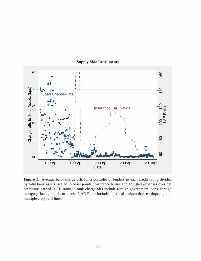
Supply-Side Instruments
Loan Charge−Offs
Insurance LAE Ratios
6080
100
120
140
160
LAE
Rat
io
01
23
45
Cha
rge−
offs
to T
otal
Ass
ets
(bps
)
1990q1 1995q1 2000q1 2005q1 2010q1Date
Figure 1: Average bank charge-offs for a portfolio of lenders to each credit rating dividedby total bank assets, scaled to basis points. Insurance losses and adjusted expenses over netpremiums earned (LAE Ratio). Bank charge-offs include foreign government loans, foreignmortgage loans, and farm loans. LAE Ratio includes medical malpractice, earthquake, andmultiple crop peril lines.
36

Average Private Debt Demand Curves by Tax Quintile
34
56
78
Yie
ld (
%)
.05 .1 .15 .2 .25Probability of Issuance
Low Tax High Tax
Figure 2: Average firm demand curves for privately-issued debt for firms in the highest andlowest quintiles of marginal tax rate. The center point on each curve is the average imputedyield paid on the security. The outer points are one standard deviation above and below theaverage imputed yield. One standard deviation in marginal tax rate is .153. One standard de-viation in imputed yield is 1.94%. The 90% confidence intervals are given around the demandcurves.
37

Average Public Debt Demand Curves by Tax Quintile
45
67
8Y
ield
(%
)
.05 .1 .15Probability of Issuance
Low Tax High Tax
Figure 3: Average firm demand curves for publicly-issued debt for firms in the highest andlowest quintiles of marginal tax rate. The center point on each curve is the average imputedyield paid on the security. The outer points are one standard deviation above and below theaverage imputed yield. One standard deviation in marginal tax rate is .153. One standarddeviation in imputed yield is 1.6%. The 90% confidence intervals are given around the demandcurves.
38

AME of Marginal Tax Rate on Demand
Lower Tax Rate
Higher Tax Rate
45
67
8Y
ield
(%
)
.05 .1 .15 .2Probability of Issuance
(a) Private Debt
Lower Tax Rate
Higher Tax Rate
45
67
8Y
ield
(%
)
.06 .08 .1 .12 .14Probability of Issuance
(b) Public Debt
Figure 4: Average marginal effect of a one standard deviation change in marginal tax rate. Thecenter point on each curve is the average imputed yield paid on the security. The outer pointsare one standard deviation above and below the average imputed yield. One standard deviationin marginal tax rate is .153. One standard deviation in imputed yield is 1.94% for private debtand 1.6% for public debt.
39

Impact of a 10% Tax Cut
Aggregate Debt
−1
−.5
0.5
1C
hang
e In
Dem
and
(%)
1990q1 1995q1 2000q1 2005q1 2010q1Date
(a) All Debt
Private Debt
Public Debt
−1
−.5
0.5
1C
hang
e In
Dem
and
(%)
1990q1 1995q1 2000q1 2005q1 2010q1Date
(b) By Type of Debt
Figure 5: Impact of a 10% tax cut on the probability of issuing debt over the sample. The 90%confidence intervals are provided around the estimated change. The demand estimates used arefrom Table 5.
40

Tab
le1:
Sum
mar
ySt
atis
tics
Out
side
Opt
ion
Priv
ate
Deb
tPu
blic
Deb
tE
quity
Mea
nSD
Mea
nSD
Mea
nSD
Mea
nSD
Mar
ket-
Lev
elVa
riab
les
Mar
ketS
hare
(%)
79.2
96.
269.
013.
658.
093.
263.
611.
28P
rodu
ct-S
peci
ficVa
riab
les
Yie
ldto
Mat
urity
(%)
5.87
2.37
7.24
2.50
Mat
urity
(Yrs
.)4.
162.
7412
.57
9.29
Cap
italR
aise
d(U
S$M
il.)
859
1,83
138
843
372
93,
104
Fir
mC
hara
cter
isti
csFi
rmSi
ze(U
S$M
il.)
5,74
715
,652
9,82
425
,184
10,9
4424
,681
4,23
39,
773
Mar
gina
lTax
Rat
e(%
)20
.64
15.4
421
.04
15.3
221
.97
15.0
619
.62
15.8
6St
atut
ory
Tax
Rat
e(%
)24
.44
16.0
025
.07
15.7
226
.00
15.1
723
.94
16.2
2M
arke
t-to
-Boo
k1.
150.
631.
170.
651.
160.
681.
701.
09Pr
ofita
bilit
y*3.
322.
143.
381.
983.
151.
953.
492.
52Pr
ofita
bilit
yD
rift
*0.
010.
130.
010.
120.
020.
100.
040.
12Pr
ofita
bilit
yV
olat
ility
*1.
161.
051.
020.
910.
940.
841.
051.
09Ta
ngib
ility
0.42
0.25
0.41
0.24
0.47
0.26
0.38
0.26
Ear
ning
sY
ield
(%)
6.83
4.01
6.80
3.82
6.49
3.81
5.23
3.43
Stoc
kR
etur
n(%
)2.
1524
.70
3.09
22.4
14.
8924
.17
13.1
531
.10
Ear
ning
sSu
rpri
seto
Pric
e*1.
8817
.30
1.46
12.5
11.
053.
180.
893.
60A
ltman
’sZ
-Sco
re0.
530.
620.
530.
570.
440.
530.
530.
70C
apit
alSt
ruct
ure
Vari
able
sC
apita
lRai
sed
toA
sset
s*18
.60
19.8
313
.06
17.3
613
.29
15.6
2L
ever
age*
39.2
620
.75
38.4
719
.33
39.8
817
.88
35.9
019
.78
Shor
t-Te
rmD
ebtt
oA
sset
s*4.
266.
614.
686.
624.
736.
063.
164.
97C
ash
toA
sset
s*6.
168.
145.
206.
535.
177.
8510
.72
13.1
3Fi
nanc
ing
Nee
d*-4
.80
9.75
-4.5
59.
33-3
.05
10.4
8-2
.45
13.0
9
Var
iabl
esw
ithan
*ar
esc
aled
bya
fact
orof
100.
All
firm
-spe
cific
vari
able
sar
em
easu
red
asof
the
prev
ious
fisca
lqua
rter
.All
ratio
sar
ew
inso
rize
dat
the
2.5
and
97.5
perc
entl
evel
sby
mar
ket.
Spec
ific
vari
able
defin
ition
sca
nbe
foun
din
App
endi
xA
.
41

Table 2: Imputed Yield
Private Debt Public DebtFinancing Need -0.018 0.133**
( 0.030) ( 0.053)Leverage 0.177*** 0.357***
( 0.036) ( 0.069)Profitability -0.114*** 0.026
( 0.035) ( 0.054)Profitability Drift 0.028 -0.120**
( 0.036) ( 0.058)Profitability Volatility 0.052 0.077
( 0.031) ( 0.058)Tangibility -0.004 0.104*
( 0.029) ( 0.059)Market-to-Book -0.100*** -0.513***
( 0.021) ( 0.057)Short Term Debt to Assets 0.058* 0.005
( 0.030) ( 0.051)Cash to Assets 0.022 -0.310***
( 0.025) ( 0.069)Altman’s Z-Score 0.014 0.209***
( 0.026) ( 0.078)Earnings Surprise -0.007 0.120
( 0.059) ( 0.064)Marginal Tax Rate -0.054*** -0.027
( 0.023) ( 0.044)Stock Return 0.006 -0.077
( 0.024) ( 0.049)Year-Quarter Fixed Effects X XCredit Rating Fixed Effects X XObservations 3,011 2,744Root MSE 0.945 1.797Adjusted R2 0.819 0.424
Estimates from yield regression. Coefficients standardized by sample standard deviations.Firm block-bootstrapped standard errors in parentheses. An * denotes significance at the tenpercent level; ** denotes significance at the five percent level; *** denotes significance at theone percent level.
42
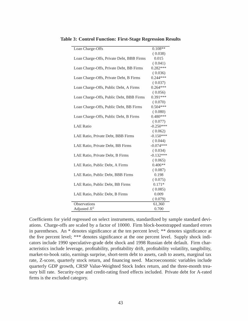
Table 3: Control Function: First-Stage Regression Results
Loan Charge-Offs 0.108**( 0.038)
Loan Charge-Offs, Private Debt, BBB Firms 0.015( 0.041)
Loan Charge-Offs, Private Debt, BB Firms 0.282***( 0.036)
Loan Charge-Offs, Private Debt, B Firms 0.244***( 0.037)
Loan Charge-Offs, Public Debt, A Firms 0.264***( 0.056)
Loan Charge-Offs, Public Debt, BBB Firms 0.391***( 0.070)
Loan Charge-Offs, Public Debt, BB Firms 0.504***( 0.080)
Loan Charge-Offs, Public Debt, B Firms 0.480***( 0.077)
LAE Ratio -0.250***( 0.062)
LAE Ratio, Private Debt, BBB Firms -0.150***( 0.044)
LAE Ratio, Private Debt, BB Firms -0.074***( 0.034)
LAE Ratio, Private Debt, B Firms -0.132***( 0.065)
LAE Ratio, Public Debt, A Firms 0.406**( 0.087)
LAE Ratio, Public Debt, BBB Firms 0.198( 0.075)
LAE Ratio, Public Debt, BB Firms 0.171*( 0.085)
LAE Ratio, Public Debt, B Firms 0.009( 0.079)
Observations 61,360Adjusted R2 0.700
Coefficients for yield regressed on select instruments, standardized by sample standard devi-ations. Charge-offs are scaled by a factor of 10000. Firm block-bootstrapped standard errorsin parentheses. An * denotes significance at the ten percent level; ** denotes significance atthe five percent level; *** denotes significance at the one percent level. Supply shock indi-cators include 1990 speculative-grade debt shock and 1998 Russian debt default. Firm char-acteristics include leverage, profitability, profitability drift, profitability volatility, tangibility,market-to-book ratio, earnings surprise, short-term debt to assets, cash to assets, marginal taxrate, Z-score, quarterly stock return, and financing need. Macroeconomic variables includequarterly GDP growth, CRSP Value-Weighted Stock Index return, and the three-month trea-sury bill rate. Security-type and credit-rating fixed effects included. Private debt for A-ratedfirms is the excluded category.
43

Table 4: Logit Estimates, Specification (1)
Private Debt Public Debt EquityLeverage -0.339* 0.349 -0.521*
( 0.181) ( 0.245) ( 0.311)Market-to-Book 0.087* 0.144** 0.632***
( 0.049) ( 0.070) ( 0.061)Earnings Surprise -0.031 -6.117*** -1.359
( 0.737) ( 1.398) ( 1.261)Short Term Debt to Assets 1.297*** 2.850*** -1.251
( 0.410) ( 0.653) ( 0.833)Cash to Assets -3.096*** -2.095*** 1.864***
( 0.400) ( 0.481) ( 0.433)Profitability 3.096** 2.845 4.203*
( 1.404) ( 1.874) ( 2.543)Profitability Drift -3.572 -63.125* 130.553***
( 22.530) ( 38.199) ( 35.223)Profitability Volatility -13.145*** -23.668*** -12.638***
( 2.661) ( 4.868) ( 4.103)Marginal Tax Rate 0.023 0.535*** 0.134
( 0.187) ( 0.207) ( 0.273)Altman’s Z-Score -0.225*** -0.353*** -0.397***
( 0.051) ( 0.067) ( 0.078)Stock Return 0.223** 0.333*** 1.190***
( 0.091) ( 0.083) ( 0.135)Financing Need 0.757*** 2.333*** 1.831***
( 0.232) ( 0.284) ( 0.369)CRSP VW Market Return -0.844*** 0.046 0.067
( 0.226) ( 0.277) ( 0.430)3-Month T-Bill -0.079*** -0.081*** 0.027
( 0.011) ( 0.013) ( 0.016)GDP Growth 0.120*** -0.025** 0.029
( 0.010) ( 0.013) ( 0.020)Debt Type Constant -1.593*** -1.623*** -3.688***
( 0.123) ( 0.150) ( 0.169)Observations 29,487Firms 1,644Pseudo R2 0.437
Estimates from conditional mixed logit regression. Coefficients under a specific security choiceare specific to that choice. Standard errors calculated by bootstrapping data by firm. An *denotes significance at the ten percent level; ** denotes significance at the five percent level;*** denotes significance at the one percent level.
44

Table 5: Logit Estimates, Specification (2)
Private Debt Public Debt EquityYield (%) -0.305***
( 0.048)Control Function 0.152**
( 0.059)Earnings Yield (%) -0.042**
( 0.018)Leverage 0.341* 0.949*** -0.511
( 0.189) ( 0.251) ( 0.313)Market-to-Book -0.033 -0.050 0.558***
( 0.055) ( 0.097) ( 0.066)Earnings Surprise 0.025 -4.994*** -1.541
( 0.510) ( 1.216) ( 1.570)Short Term Debt to Assets 1.169*** 2.821*** -0.991
( 0.446) ( 0.665) ( 0.866)Cash to Assets -2.369*** -3.221*** 1.904***
( 0.412) ( 0.526) ( 0.432)Profitability 1.555 3.314* 6.066**
( 1.582) ( 1.927) ( 2.736)Profitability Drift 22.535 -84.381** 133.487***
( 30.727) ( 42.164) ( 33.245)Profitability Volatility -8.619*** -19.012*** -11.169***
( 3.048) ( 5.103) ( 4.046)Marginal Tax Rate 0.750* -1.748** 0.207
( 0.408) ( 0.686) ( 0.279)Yield Interaction -0.195*** 0.363***
( 0.073) ( 0.108)Altman’s Z-Score -0.223*** -0.222*** -0.371***
( 0.052) ( 0.066) ( 0.081)Stock Return 0.226** 0.241*** 1.138***
( 0.097) ( 0.089) ( 0.135)Financing Need 0.797*** 2.783*** 1.753***
( 0.250) ( 0.320) ( 0.361)CRSP VW Market Return -0.915*** -0.281 0.005
( 0.263) ( 0.291) ( 0.439)3-Month T-Bill 0.210*** -0.003 0.035**
( 0.038) ( 0.026) ( 0.018)GDP Growth 0.088*** -0.054*** 0.024
( 0.013) ( 0.015) ( 0.021)Debt Type Constant -0.973*** 0.056 -3.478***
( 0.199) ( 0.326) ( 0.202)Observations 29,487Firms 1,644Pseudo R2 0.439
Estimates from conditional mixed logit regression. Coefficients under a specific security choiceare specific to that choice. Standard errors calculated by bootstrapping data by firm. An *denotes significance at the ten percent level; ** denotes significance at the five percent level;*** denotes significance at the one percent level.
45

Table 6: Logit Estimates, Specification (3)
Private Debt Public Debt EquityYield (%) -0.378***
( 0.042)Control Function 0.198***
( 0.042)Earnings Yield (%) -0.045***
( 0.017)Leverage 0.411** 1.787*** -0.807**
( 0.205) ( 0.255) ( 0.324)Market-to-Book -0.037 -0.179** 0.624***
( 0.052) ( 0.087) ( 0.069)Earnings Surprise 0.042 -2.717*** -2.082
( 0.447) ( 0.838) ( 1.708)Short Term Debt to Assets 1.335*** 1.976*** 0.075
( 0.489) ( 0.627) ( 0.760)Cash to Assets -2.311*** -2.506*** 1.298***
( 0.412) ( 0.540) ( 0.432)Profitability 1.249 3.133 5.833**
( 1.624) ( 1.996) ( 2.770)Profitability Drift 25.327 -66.125 112.360***
( 32.498) ( 43.936) ( 30.335)Profitability Volatility -8.000*** -13.972*** -11.565***
( 2.993) ( 5.103) ( 3.861)Marginal Tax Rate 0.808 -2.262*** 0.383
( 0.442) ( 0.654) ( 0.266)Yield Interaction -0.213*** 0.387***
( 0.078) ( 0.099)Altman’s Z-Score -0.218*** -0.267*** -0.289***
( 0.052) ( 0.066) ( 0.079)Stock Return 0.214** 0.307*** 1.049***
( 0.098) ( 0.092) ( 0.125)Financing Need 0.772*** 3.130*** 1.496***
( 0.259) ( 0.352) ( 0.355)CRSP VW Market Return -0.912*** -0.469 0.093
( 0.271) ( 0.296) ( 0.440)3-Month T-Bill 0.274*** 0.016 0.040**
( 0.036) ( 0.022) ( 0.018)GDP Growth 0.082*** -0.059*** 0.021
( 0.015) ( 0.016) ( 0.021)Debt Type Constant -0.958*** 0.853*** -4.095***
( 0.183) ( 0.300) ( 0.227)BBB Market FE 0.186*** -0.384*** 0.472***
( 0.069) ( 0.072) ( 0.125)BB Market FE 0.219*** -0.719*** 0.817***
( 0.084) ( 0.095) ( 0.124)B Market FE 0.140 -1.057*** 0.823***
( 0.089) ( 0.120) ( 0.175)Observations 29,487Firms 1,644Pseudo R2 0.442
Estimates from conditional mixed logit regression. Coefficients under a specific security choiceare specific to that choice. Standard errors calculated by bootstrapping data by firm. An *denotes significance at the ten percent level; ** denotes significance at the five percent level;*** denotes significance at the one percent level.
46
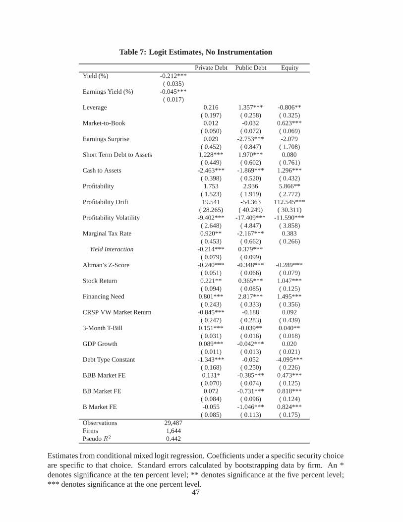
Table 7: Logit Estimates, No Instrumentation
Private Debt Public Debt EquityYield (%) -0.212***
( 0.035)Earnings Yield (%) -0.045***
( 0.017)Leverage 0.216 1.357*** -0.806**
( 0.197) ( 0.258) ( 0.325)Market-to-Book 0.012 -0.032 0.623***
( 0.050) ( 0.072) ( 0.069)Earnings Surprise 0.029 -2.753*** -2.079
( 0.452) ( 0.847) ( 1.708)Short Term Debt to Assets 1.228*** 1.970*** 0.080
( 0.449) ( 0.602) ( 0.761)Cash to Assets -2.463*** -1.869*** 1.296***
( 0.398) ( 0.520) ( 0.432)Profitability 1.753 2.936 5.866**
( 1.523) ( 1.919) ( 2.772)Profitability Drift 19.541 -54.363 112.545***
( 28.265) ( 40.249) ( 30.311)Profitability Volatility -9.402*** -17.409*** -11.590***
( 2.648) ( 4.847) ( 3.858)Marginal Tax Rate 0.920** -2.167*** 0.383
( 0.453) ( 0.662) ( 0.266)Yield Interaction -0.214*** 0.379***
( 0.079) ( 0.099)Altman’s Z-Score -0.240*** -0.348*** -0.289***
( 0.051) ( 0.066) ( 0.079)Stock Return 0.221** 0.365*** 1.047***
( 0.094) ( 0.085) ( 0.125)Financing Need 0.801*** 2.817*** 1.495***
( 0.243) ( 0.333) ( 0.356)CRSP VW Market Return -0.845*** -0.188 0.092
( 0.247) ( 0.283) ( 0.439)3-Month T-Bill 0.151*** -0.039** 0.040**
( 0.031) ( 0.016) ( 0.018)GDP Growth 0.089*** -0.042*** 0.020
( 0.011) ( 0.013) ( 0.021)Debt Type Constant -1.343*** -0.052 -4.095***
( 0.168) ( 0.250) ( 0.226)BBB Market FE 0.131* -0.385*** 0.473***
( 0.070) ( 0.074) ( 0.125)BB Market FE 0.072 -0.731*** 0.818***
( 0.084) ( 0.096) ( 0.124)B Market FE -0.055 -1.046*** 0.824***
( 0.085) ( 0.113) ( 0.175)Observations 29,487Firms 1,644Pseudo R2 0.442
Estimates from conditional mixed logit regression. Coefficients under a specific security choiceare specific to that choice. Standard errors calculated by bootstrapping data by firm. An *denotes significance at the ten percent level; ** denotes significance at the five percent level;*** denotes significance at the one percent level.
47

Table 8: Probability of Issuing Debt
Panel A: Average Marginal EffectSpecification (1) (2) (3)Private Debt
Marginal Tax Rate -0.06 -0.51** -0.52**( 0.25) ( 0.24) ( 0.24)
Yield (%) -6.34*** -7.75***( 0.85) ( 0.75)
Public DebtMarginal Tax Rate 0.67*** 0.65** 0.18
( 0.24) ( 0.27) ( 0.29)Yield (%) -3.01*** -3.88***
( 0.74) ( 0.57)Control Variables
Firm Characteristics X X XMacro Variables X X XCredit Rating FEs X
Panel B: Relative Average Marginal EffectSpecification (1) (2) (3)Private Debt
Marginal Tax Rate -0.54 -5.38** -5.56**( 2.45) ( 2.30) ( 2.30)
Yield (%) -59.65**8 -72.91***( 8.15) ( 7.29)
Public DebtMarginal Tax Rate 7.31*** 7.72** 2.62
( 2.80) ( 3.05) ( 3.23)Yield (%) -33.32*** -43.18***
( 8.01) ( 6.29)Control Variables
Firm Characteristics X X XMacro Variables X X XCredit Rating FEs X
Panel A presents the average marginal effect of a one standard deviation change in the marginaltax rate and imputed yield (in %). Panel B presents the relative average marginal effect of aone standard deviation change in the marginal tax rate and imputed yield (in %). The relativeaverage marginal effect is the percent change in probability of issuance; the average marginaleffect is the percentage-point change in probability of issuance. Specification 3 includes creditrating fixed effects. Standard errors in parentheses. An * denotes significance at the ten percentlevel; ** denotes significance at the five percent level; *** denotes significance at the onepercent level.
48

Table 9: Probability of Issuing Debt, Alternate Tax Measure
Panel A: Average Marginal EffectSpecification (1) (2) (3)Private Debt
Statutory Tax Rate 0.34 -0.05 -0.00( 0.21) ( 0.21) ( 0.23)
Yield (%) -7.06*** -8.74***( 0.88) ( 0.86)
Public DebtStatutory Tax Rate 0.95*** 0.90*** 0.43
( 0.24) ( 0.27) ( 0.30)Yield (%) -3.52*** -4.35***
( 0.72) ( 0.64)Control Variables
Firm Characteristics X X XMacro Variables X X XCredit Rating FEs X
Panel B: Relative Average Marginal EffectSpecification (1) (2) (3)Private Debt
Statutory Tax Rate 3.27* -0.95 -0.60( 1.96) ( 2.03) ( 2.16)
Yield (%) -65.95*** -81.68***( 8.26) ( 8.07)
Public DebtStatutory Tax Rate 10.41*** 10.19*** 5.21
( 2.81) ( 2.95) ( 3.25)Yield (%) -38.79*** -48.20***
( 7.90) ( 7.05)Control Variables
Firm Characteristics X X XMacro Variables X X XCredit Rating FEs X
Panel A presents the average marginal effect of a one standard deviation change in the statutorytax rate and imputed yield (in %). Panel B presents the relative average marginal effect of aone standard deviation change in the statutory tax rate and imputed yield (in %). The relativeaverage marginal effect is the percent change in probability of issuance; the average marginaleffect is the percentage-point change in probability of issuance. Specification 3 includes creditrating fixed effects. Standard errors in parentheses. An * denotes significance at the ten percentlevel; ** denotes significance at the five percent level; *** denotes significance at the onepercent level.
49

Table 10: Cost of Debt Sensitivity
Panel A: Average Marginal EffectSpecification (1) (2) (3)Private Debt
Marginal Tax Rate -0.14 -0.14( 0.12) ( 0.13)
Public DebtMarginal Tax Rate 0.35** 0.45***
( 0.15) ( 0.14)Control Variables
Firm Characteristics X X XMacro Variables X X XCredit Rating FEs XPanel B: Relative Average Marginal Effect
Specification (1) (2) (3)Private Debt
Marginal Tax Rate 3.90 2.80( 4.10) ( 3.52)
Public DebtMarginal Tax Rate -18.58 -18.23*
( 18.46) ( 9.96)Control Variables
Firm Characteristics X X XMacro Variables X X XCredit Rating FEs X
Panel A presents the average marginal effect of a one standard deviation change in the marginaltax rate and imputed yield (in %). Panel B presents the relative average marginal effect of aone standard deviation change in the marginal tax rate and imputed yield (in %). The relativeaverage marginal effect is the percent change in probability of issuance; the average marginaleffect is the percentage-point change in probability of issuance. Specification 3 includes creditrating fixed effects. Standard errors in parentheses. An * denotes significance at the ten percentlevel; ** denotes significance at the five percent level; *** denotes significance at the onepercent level.
50

Table 11: Quantity of Debt Chosen
100 ∗ (ΔDebtt/Assetst−1)Specification
(1) (2) (3)Marginal Tax Rate 0.07** 0.07** 0.03
( 0.03) ( 0.03) ( 0.04)Yield (%) 0.07 -0.47**
( 0.06) ( 0.23)Control Variables
Firm Characteristics X X XMacro Variables X X X2SLS X
The marginal effect of a one standard deviation change in the marginal tax rate and imputedyield (in %) on the change in the firm’s total debt, scaled by lagged book assets. Specification 1does not include the pre-tax cost of debt. Specification 2 includes the pre-tax cost of debt withno instrumentation. Specification 3 instruments the cost of debt using a two-stage least squaresprocedure with loan charge-offs and LAE ratios as instruments. Standard errors in parentheses.An * denotes significance at the ten percent level; ** denotes significance at the five percentlevel; *** denotes significance at the one percent level.
51