How Do Premium Subsidies Affect Crop Insurance Demand at Different Coverage Levels:

the Case of Corn

Jing Yi

Department of Agricultural Economics

Texas A&M University

yijing@tamu.edu

James W. Richardson

Department of Agricultural Economics

Texas A&M University

jwrichardson@tamu.edu

Henry L. Bryant

Department of Agricultural Economics

Texas A&M University

h-bryant@tamu.edu

Selected Poster/Paper prepared for presentation at the Agricultural & Applied Economics

Association’s 2016 AAEA Annual Meeting, Boston, Massachusetts, July 31-August 2, 2016

Copyright 2016 by Jing Yi; James W. Richardson; Henry L. Bryant. All rights reserved. Readers may

make verbatim copies of this document for non-commercial purposes by any means, provided that this

copyright notice appears on all such copies.

How Do Premium Subsidies Affect Crop InsuranceDemand at Different Coverage Levels: the Case of

Corn

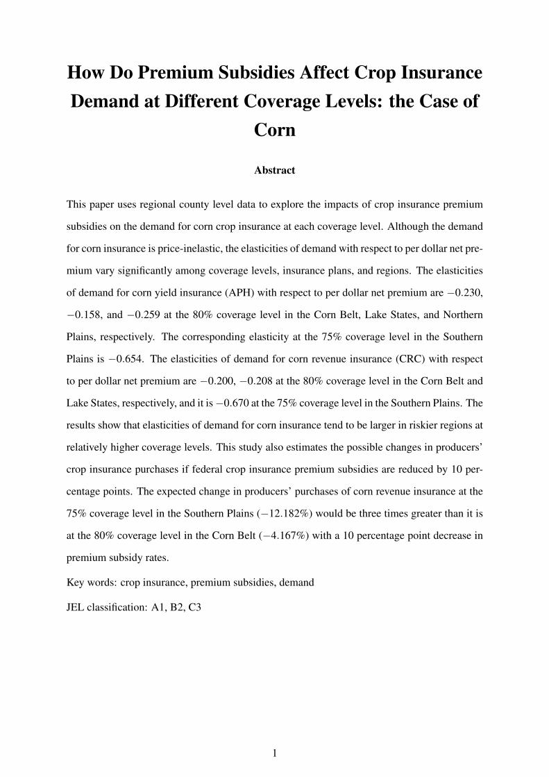
Abstract

This paper uses regional county level data to explore the impacts of crop insurance premium

subsidies on the demand for corn crop insurance at each coverage level. Although the demand

for corn insurance is price-inelastic, the elasticities of demand with respect to per dollar net pre-

mium vary significantly among coverage levels, insurance plans, and regions. The elasticities

of demand for corn yield insurance (APH) with respect to per dollar net premium are −0.230,

−0.158, and −0.259 at the 80% coverage level in the Corn Belt, Lake States, and Northern

Plains, respectively. The corresponding elasticity at the 75% coverage level in the Southern

Plains is −0.654. The elasticities of demand for corn revenue insurance (CRC) with respect

to per dollar net premium are −0.200, −0.208 at the 80% coverage level in the Corn Belt and

Lake States, respectively, and it is −0.670 at the 75% coverage level in the Southern Plains. The

results show that elasticities of demand for corn insurance tend to be larger in riskier regions at

relatively higher coverage levels. This study also estimates the possible changes in producers’

crop insurance purchases if federal crop insurance premium subsidies are reduced by 10 per-

centage points. The expected change in producers’ purchases of corn revenue insurance at the

75% coverage level in the Southern Plains (−12.182%) would be three times greater than it is

at the 80% coverage level in the Corn Belt (−4.167%) with a 10 percentage point decrease in

premium subsidy rates.

Key words: crop insurance, premium subsidies, demand

JEL classification: A1, B2, C3

1

Introduction

The U.S. Federal Crop Insurance Program (FCIP) plays a critical part in providing farmers

protection against agricultural risk. The federal crop insurance subsidies have been increased

through several policies to encourage crop insurance participation. Figure 1 shows the

corn insured acres and the federal premium subsidies in 1989 to 2013. Despite the higher

participation with higher premium subsidies, this program has been criticized as inefficient

because of the heavy government expenditure (see figure 1) and poor actuarial performance

(Glauber 2004). Figure 2 presents the loss ratio (the ratio of indemnities to gross premium)

and adjusted loss ratio (the ratio of indemnities to net premium) for the FCIP over all crops.

On average, the adjusted loss ratio is 2.07 over 2000 - 2013, which means producers tend to

collect $2.07 in indemnity payments for each dollar of their premium payment. Therefore,

understanding the effects of subsidies on demand is essential for policy makers and private

sectors.

Figure 1. Federal Premium Subsidies and Insured Acres for the U.S. Corn Crop Insur-ance ProgramSource: USDA, Risk Management Agency, Summary of Business files, 1989-2014.

Although the demand for crop insurance has been explored by many studies, the majority

of the existing studies did not report the demand for crop insurance premium at each coverage

level. Consequently, it is not clear whether there are differences among the price elasticities

of crop insurance demand across coverage levels. The two known studies which account for

the differences across coverage levels show that the demand for grape insurance in eleven

2

Figure 2. Loss Ratio and Adjusted Loss Ratio for the U.S. Crop Insurance ProgramSource: Glauber and Collins 2002.

California counties is price-elastic at the catastrophic (CAT) level of insurance. However, the

demand for grape insurance is price-inelastic among higher coverage levels (Knox and Richards

1999; Richards 2000). From the grape insurance evidence, we hypothesize that the demand for

crop insurance at each coverage level could be significant different although previous studies

show that the aggregated demand for the federal crop insurance is price-inelastic. Moreover,

because the federal premium subsidy rates are specified at each coverage level, disaggregated

demand analysis of crop insurance could provide more detailed information for policy makers

and private sectors. This study is the first one that differentiates the demand for corn insurance

policies across coverage levels, insurance policies (yield and revenue insurance policies), and

regions.

Background

To encourage higher participation, crop insurance premium subsidies were increased by the

Agricultural Risk Protection Act (ARPA) of 2000 (Babcock, Hart, and Hayes 2004; Coble

and Barnett 2013). According to Babcock and Hart (2005), ”One of the policy objectives of

the ARPA was to induce producers to buy more insurance coverage in which one measure of

more insurance is the proportion of acres insured at levels greater than 65%.” Table 1 provides

a comparison between the percentages of the premium paid by the FCIC at various coverage

levels at 100% of price coverage pre- and post- ARPA. For corn insurance, coverage is available

3

in 5% increments from 50% to 85%. Before the ARPA, the dollar amount of subsidies were

the same among coverage levels higher than or equal to 65%. The constant dollar amount of

subsidies was accomplished by setting different subsidy rates at each coverage level (Babcock

and Hart 2005). Under the ARPA, the increase in the insurance premium at higher coverage

levels was generally less than the associated increase in subsidy rates. Therefore, producers

would benefit more from purchasing higher coverage levels (Babcock, Hart, and Hayes 2004).

Another significant change is that the subsidy level, as a percentage of the full premium, is the

same for both the yield insurance program (APH) and the revenue polices (CRC) under the

ARPA. Besides, the administrative fee for CAT insurance was increased from $50 to $100 per

crop per county (Kelley 2001).

Table 1. Basic Unit Subsidy Levels Pre- and Post-ARPA

Coverage Level Pre-ARPA Post-ARPA

APH CRC

50/100 55% 42% 67%

65/100 42% 32% 59%

70/100 32% 25% 59%

75/100 24% 18% 55%

85/100 13% 10% 38%

Source: Kelly 2001; Jose 2001.

Although ARPA was implemented in 2000, it remains the most recent and broadest reform

in crop insurance premium (O’Donoghue 2014). Furthermore, there are very few studies which

explore the impacts of subsidy changes on crop insurance demand and none of them differenti-

ated coverage levels and plans. Therefore, this study examines the demand for crop insurance

at each coverage level and insurance plan.

Empirical Modeling Framework

Expected utility maximization is usually the theoretical framework in which the determinants

of insurance purchases are examined. A representative producer is subject to constraints im-

posed by characteristics of marketing and production environment, such as commodity prices.

Following Goodwin (1993), the maximization of the expected utility yields a linear equation,

4

which is a function of the representative producers risk attitudes, and the production and mar-

keting characteristics. The demand for corn insurance is given by

yi = α +Xβi + εi

where yi is the insurance purchase decision made by the producer under the utility maximization

problem. Xi is a vector of factors that influence the expected utility of insurance and εi is a

random error term.

Following Gardner and Kramer (1986) and Goodwin (1993), each county is treated as a

representative farm. Although the utilization of county-level data could reduce the variation,

compared to farm-level data, given the data availability, the county-level dataset is the best one

which can be used for estimating of crop insurance demand.

The term defined to quantify the crop insurance demand varies in previous studies, such as

the percentage of insured acres used in Gardner and Kramer (1986), and premium less expected

indemnities per dollar of liability in Cannon and Barnett (1995). In this study, the quantity

variable is constructed as the per dollar liabilities (liabilities divided by projected prices) per

enrolled acre. Liabilities are the amount of indemnities if all losses occur, and are determined

by the production conditions of insured acres, the product of insured acres, the projected price

of the product. As Goodwin (1993) mentioned, the liability should be the true measure of

the level of insurance. In Goodwin (1993) , the dependent variable is the liability per planted

acre of corn. However, insured acres should be preferred to the planted acres to adjust liabilities

because liabilities are determined by the characteristics of the insured acres, not the total planted

acres, and the total corn planted acres are also controlled in the model. Moreover, the liabilities

per enrolled acres are divided by the corn projected price in each county to estimate the per

dollar purchases.

The definitions of the price variable in the analysis of crop insurance demand are as diverse

as the measure of the quantity. The premium rate per acre is a commonly used term to measure

the cost of insurance, such as in Smith and Baquet (1996). In this study, the normalized net

premium (gross premium less subsidies) per insured acre divided by the projected price is used

to estimate the cost of insurance per insured dollar. The premium per acre is the acre unit

5

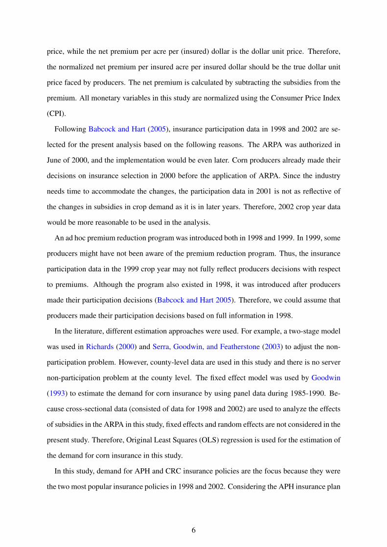
price, while the net premium per acre per (insured) dollar is the dollar unit price. Therefore,

the normalized net premium per insured acre per insured dollar should be the true dollar unit

price faced by producers. The net premium is calculated by subtracting the subsidies from the

premium. All monetary variables in this study are normalized using the Consumer Price Index

(CPI).

Following Babcock and Hart (2005), insurance participation data in 1998 and 2002 are se-

lected for the present analysis based on the following reasons. The ARPA was authorized in

June of 2000, and the implementation would be even later. Corn producers already made their

decisions on insurance selection in 2000 before the application of ARPA. Since the industry

needs time to accommodate the changes, the participation data in 2001 is not as reflective of

the changes in subsidies in crop demand as it is in later years. Therefore, 2002 crop year data

would be more reasonable to be used in the analysis.

An ad hoc premium reduction program was introduced both in 1998 and 1999. In 1999, some

producers might have not been aware of the premium reduction program. Thus, the insurance

participation data in the 1999 crop year may not fully reflect producers decisions with respect

to premiums. Although the program also existed in 1998, it was introduced after producers

made their participation decisions (Babcock and Hart 2005). Therefore, we could assume that

producers made their participation decisions based on full information in 1998.

In the literature, different estimation approaches were used. For example, a two-stage model

was used in Richards (2000) and Serra, Goodwin, and Featherstone (2003) to adjust the non-

participation problem. However, county-level data are used in this study and there is no server

non-participation problem at the county level. The fixed effect model was used by Goodwin

(1993) to estimate the demand for corn insurance by using panel data during 1985-1990. Be-

cause cross-sectional data (consisted of data for 1998 and 2002) are used to analyze the effects

of subsidies in the ARPA in this study, fixed effects and random effects are not considered in the

present study. Therefore, Original Least Squares (OLS) regression is used for the estimation of

the demand for corn insurance in this study.

In this study, demand for APH and CRC insurance policies are the focus because they were

the two most popular insurance policies in 1998 and 2002. Considering the APH insurance plan

6

provides yield protection for corn producers, while the CRC insurance plan provides revenue

protection, demand estimation is seperated for different insurance policies.

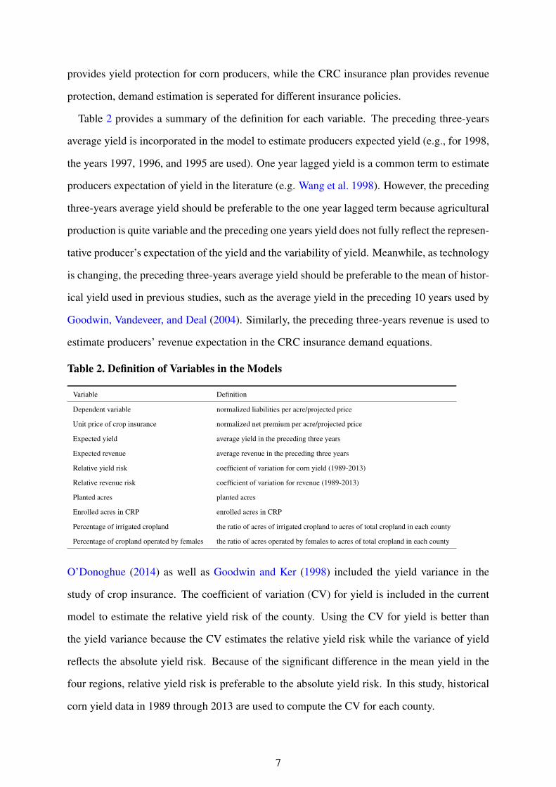
Table 2 provides a summary of the definition for each variable. The preceding three-years

average yield is incorporated in the model to estimate producers expected yield (e.g., for 1998,

the years 1997, 1996, and 1995 are used). One year lagged yield is a common term to estimate

producers expectation of yield in the literature (e.g. Wang et al. 1998). However, the preceding

three-years average yield should be preferable to the one year lagged term because agricultural

production is quite variable and the preceding one years yield does not fully reflect the represen-

tative producer’s expectation of the yield and the variability of yield. Meanwhile, as technology

is changing, the preceding three-years average yield should be preferable to the mean of histor-

ical yield used in previous studies, such as the average yield in the preceding 10 years used by

Goodwin, Vandeveer, and Deal (2004). Similarly, the preceding three-years revenue is used to

estimate producers’ revenue expectation in the CRC insurance demand equations.

Table 2. Definition of Variables in the Models

Variable Definition

Dependent variable normalized liabilities per acre/projected price

Unit price of crop insurance normalized net premium per acre/projected price

Expected yield average yield in the preceding three years

Expected revenue average revenue in the preceding three years

Relative yield risk coefficient of variation for corn yield (1989-2013)

Relative revenue risk coefficient of variation for revenue (1989-2013)

Planted acres planted acres

Enrolled acres in CRP enrolled acres in CRP

Percentage of irrigated cropland the ratio of acres of irrigated cropland to acres of total cropland in each county

Percentage of cropland operated by females the ratio of acres operated by females to acres of total cropland in each county

O’Donoghue (2014) as well as Goodwin and Ker (1998) included the yield variance in the

study of crop insurance. The coefficient of variation (CV) for yield is included in the current

model to estimate the relative yield risk of the county. Using the CV for yield is better than

the yield variance because the CV estimates the relative yield risk while the variance of yield

reflects the absolute yield risk. Because of the significant difference in the mean yield in the

four regions, relative yield risk is preferable to the absolute yield risk. In this study, historical

corn yield data in 1989 through 2013 are used to compute the CV for each county.

7

The total corn planted acres are incorporated in the model since a potential correlation is

expected between the planted acres and the insurance purchases. The enrolled acres of CRP

are used as an independent variable because it is impossible to purchase insurance protection

for acres enrolled in the CRP. The percentage of irrigated cropland in each county is controlled

in the model as this item could reflect the production environment and affect the distribution

of yield. Women tend to be more risk averse than men (Charness and Gneezy 2012), thus the

percentage of cropland operated by females is also incorporated in the equations.

Data

The data utilized in this analysis were drawn from three major sources. The primary data

source is USDA, Risk Management Agency (RMA) administrative data. The individual data

are aggregated to the county-level by crop type and crop insurance policy at each coverage

level. Information about insured acres, total premium, liabilities, and subsidies is available

from RMA’s Summary of Business Report (SBR) publications. The SBR publications report

participation data from 1989 through 2014 and contain spatially identifying information. Thus

the participation data can be combined with other datasets. There are about 2,000 observations

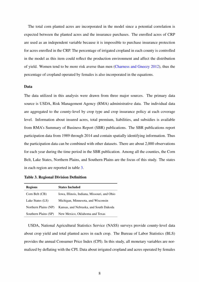
for each year during the time period in the SBR publication. Among all the counties, the Corn

Belt, Lake States, Northern Plains, and Southern Plains are the focus of this study. The states

in each region are reported in table 3.

Table 3. Regional Division Definition

Regions States Included

Corn Belt (CB) Iowa, Illinois, Indiana, Missouri, and Ohio

Lake States (LS) Michigan, Minnesota, and Wisconsin

Northern Plains (NP) Kansas, and Nebraska, and South Dakoda

Southern Plains (SP) New Mexico, Oklahoma and Texas

USDA, National Agricultural Statistics Service (NASS) surveys provide county-level data

about crop yield and total planted acres in each crop. The Bureau of Labor Statistics (BLS)

provides the annual Consumer Price Index (CPI). In this study, all monetary variables are nor-

malized by deflating with the CPI. Data about irrigated cropland and acres operated by females

8

and males are obtained from National Agricultural Statistics Services (NASS)s 1997 and 2002

Censuses of Agriculture. County-level data on participation in Conservation Reserve Program

(CRP) is collected from USDA, Farm Service Agency (FSA) to estimate the effect of CRP

acreage on insurance demand.

Demand Estimation

Breusch-Pagan (1979) and Cook-Weisberg (1983) test is applied to test for heteroskedasticity.

The variances of error are all equal is assumed in the null hypothesis of the Breusch-Pagan and

Cook-Weisberg test. If the regression is rejected by the null hypothesis at the 95% confidence

interval, the robust standard errors are used in the regression. Variance inflation factors (VIF)

are used to diagnose collinearity problems. Among all the estimations, the highest VIF is less

than 10. Therefore, multicollinearity does not appear to be a considerable problem.

Link tests are applied to test for model specification. The basic idea of the link test is that

any additional independent variable should be statistically insignificant if the model is correctly

specified (Bruin 2006). According to Bruin (2006), the link test creates two variables: predicted

dependent variable (y) and the square of the predicted dependent variable (y2). The model is

refit only using these two variables as predictors. In this study, the results of link tests suggest

that models for APH insurance are well specified excepted at the 55% and 60% coverage levels

in the Corn Belt, at the 65%, 70%, and 80% coverage levels in the Lake States, at the 50%

coverage level in the Northern Plains, and at the 65% coverage level in the Southern Plains.

To address the misspecification problem, linear-linear models are used at the 55% and 60%

coverage levels in the Corn Belt, the linear-log models are used at the 65%, 70%, and 80%

coverage levels in the Lake States, the linear-log model is used at the 50% coverage level in

the Northern Plains, and the log-linear model is used at the 65% coverage level in the Southern

Plains. The estimations for corn CRC insurance at the 75% and 80% coverage levels in the

Corn Belt and at 65%, 70% and 75% coverage levels in the Northern Plains are rejected by the

null hypothesis of link tests at the 95% confidence interval. To deal with the misspecification

problem, linear-linear models are used at the two coverage levels (75% and 80%) in the Corn

Belt, and log-log, linear-log, and linear-linear models are used at the 65%, 70%, and 75%

coverage levels in the Northern Plains, respectively.

9

The Demand Estimation for Corn APH Insurance

In the Lake States, there are only nine observations at the 85% coverage level, which results

in limited power for the F-test (0.30). Among all the other coverage levels and regions, the p-

values of the F-tests are zero to four decimal places, which mean that the models are statistically

significant. the coefficients of determination, or R2, range from 0.399 (at the 80% coverage

level in the Northern Plains) to 0.894 (at the 75% coverage level in the Southern Plains), which

suggests that the model could explain from 39.9% to 89.4% of the total variation in the demand

for liabilities by the variation in the independent variables. The results indicate that explanatory

variables explain the demand for corn APH insurance fairly well.

The Demand Estimation for Corn CRC Insurance

Overall, the model explains the demand for corn CRC insurance fairly well. The coefficients

of determination, or R2, range from 0.227 (for 55% coverage level in the Northern Plains)

to 0.946 (for 55% coverage level in the Southern Plains) which suggest that the model could

explain from 22.7% to 94.6% of the total variation in the demand of per dollar liabilities by

the variation in the independent variables. The F-tests are statistically significant (p-values

are zero to four decimal places) except for the 85% coverage level in the Lake States and the

55% coverage level in the Northern Plains (the p-value of the F-test is 0.5352 and 0.0288,

respectively).

Elasticities of Demand

The elasticities of corn APH and CRC insurance with respect to per dollar net premium are

summarized in table 4 (the elasticities of demand for corn APH and CRC insurance with re-

spect to each independent variable are reported in tables 6 through 13). The elasticities of de-

mand for corn APH insurance with respect to per dollar net premium are −0.230, −0.158, and

−0.259 at the 80% coverage level in the Corn Belt, Lake States, and Northern Plains, respec-

tively. The corresponding elasticity at the 75% coverage level in the Southern Plains is −0.654.

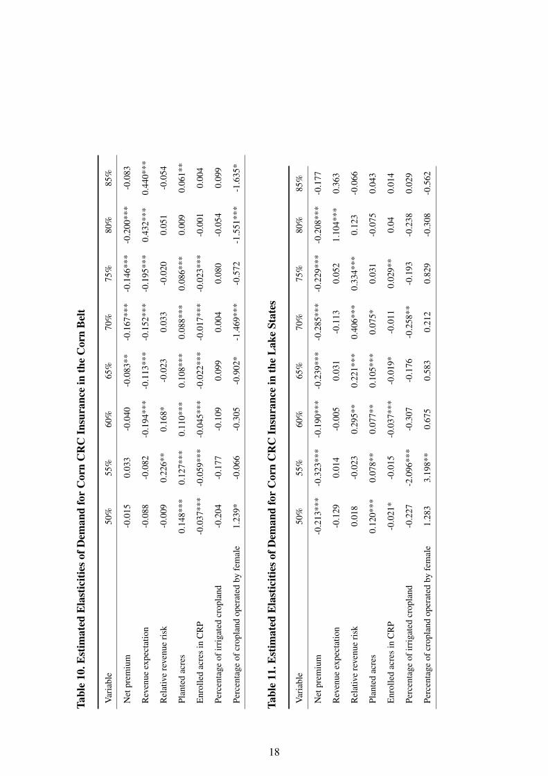
The elasticities of demand for corn CRC insurance with respect to per dollar net premium are

−0.200, −0.208 at the 80% coverage level in the Corn Belt and Lake States, respectively, and

it is −0.670 at the 75% coverage level in the Southern Plains. The results show that elasticities

10

of demand for corn insurance tend to be larger in riskier regions at relatively higher coverage

levels. The results show the importance of separating coverage levels, regions, and insurance

plans in the study for crop insurance demand, which were not reported in previous studies.

Table 4. Estimated Elasticities of Demand for APH and CRC Insurance With Respect to

Per Dollar of Net Premium

Region Policy 50% 55% 60% 65% 70% 75% 80% 85%

Corn BeltAPH -0.047** -0.028 -0.106*** -0.114*** -0.137*** -0.149*** -0.230*** 0.017

CRC -0.015 0.033 -0.040 -0.083** -0.167*** -0.146*** -0.200*** -0.083

Lake StatesAPH -0.180*** -0.138*** -0.138*** -0.147*** -0.094** -0.157*** -0.158**

CRC -0.213*** -0.323*** -0.190*** -0.239*** -0.285*** -0.229*** -0.208*** -0.177

Northern PlainsAPH -0.170*** -0.004 -0.305*** -0.038 -0.097 -0.188* -0.259** -0.284**

CRC -0.042 -0.205 -0.290*** 0.017 -0.044 0.097 0.075 0.009

Southern PlainsAPH -0.221** -0.131 -0.248* -0.227** -0.155 -0.654***

CRC -0.331** -0.094 -0.373*** -0.242* -0.501*** -0.670***

The negative correlation between the per dollar net premium and the amount of per dollar

liability purchases (table 4) is consistent with theoretical expectations, and the magnitude of

elasticities of demand for crop insurance with respect to price is basically consistent with results

reported in other studies. The estimated average demand elasticities for liability per planted

acre are -0.73 in Iowa in Goodwin (1993), -0.24 in the Heartland in Goodwin (2001), -0.13 in

Illinois, Idaho, Iowa, and Ohio in O’Donoghue (2014). Because this study is the only one which

separated coverage levels in the analysis of corn insurance demand, it is difficult to compare the

estimated elasticities of corn insurance demand at each coverage level with existing studies at

each coverage level. But overall, the elasticities derived in this analysis are generally consistent

with results estimated in previous studies.

The elasticities of demand with respect to per dollar net premium vary across coverage levels.

For example, in the Corn Belt (table 4), the elasticity of demand for corn yield insurance with

respect to per dollar net premium at the 50% coverage level is small (−0.047), and the elasticity

at the 55% is statistically insignificant (-0.028). The results in table 4 imply that corn producers

in the Corn Belt are not likely to significantly change their demand for corn APH insurance

at the 50% and 55% coverage levels due to the changes in subsidies. These producers may

purchase the low coverage levels to meet the requirements for loan applications. As shown in

11

table 4, the price elasticities are statistically significant but inelastic at the 60%, 65%, 70%,

75%, and 80% coverage levels ( 0.106, 0.114, 0.137, 0.149, 0.230, respectively). Although

they are all price-inelastic, the elasticity at 80% coverage level (-0.230) is about five times of

the elasticity at the 50% coverage level (-0.047). The results imply that producers are more

sensitive to changes in premium at high coverage levels (e.g. 80% coverage level) than low

coverage levels (e.g. 50% and 55%) in the Corn Belt. The results also prove the importance of

differentiating coverage levels in the analysis of demand for corn insurance (table 4).

Results in table 4 also suggest that producers in riskier regions are more responsive to the

change of per dollar net premium. For instance, with a 1% decrease in the per dollar net pre-

mium, producers in the Corn Belt would increase their purchase for corn APH insurance at the

50% coverage level by 0.047%, while producers in the Southern Plains would increase the pur-

chase by 0.221%. So the change in the Southern Plains is quadrupled compared to the change

in the Corn Belt. In O’Donoghue (2014), the elasticities of demand for corn insurance mea-

sured as liabilities per acre are −0.13, −0.24, and −0.25 in the Midwest, Lake, and Northern

Plains, respectively, which also exhibit the patterns that producers in riskier regions tend to be

more responsive to corn insurance, although the pattern was not mentioned in his study.

The elasticities of demand for insurance with respect to per dollar net premium not only

change across coverage levels and regions, but the elasticities also change between insurance

plans (table 4). In the Corn Belt and Northern Plains, the demand for corn APH insurance

is more price responsive than the demand for corn CRC insurance, while the elasticities of

demand for corn CRC insurance with respect to per dollar net premium are larger than the

corresponding elasticities for corn APH insurance in the Lake States and Southern Plains. For

example, in the Southern Plains, the elasticity of corn APH insurance with respect to per dollar

net premium is 0.248, while the corresponding elasticity for corn CRC insurance is 0.373 at the

60% coverage (table 4).

Results presented in table 4 indicate the necessity for separating insurance plans, regions, and

coverage levels in the analysis of corn insurance demand, which was overlooked in previous

studies. The elasticity of demand for CRC insurance at the 75% coverage level in the Southern

Plains is −0.670, which is more than 14 times of the elasticity of demand for APH insurance at

12

the 50% in the Corn Belt (−0.047). Although the elasticities are price-inelastic, a 1% change in

the net premium would induce 14 times larger effect at the 75% coverage level in the Southern

Plains than the effect at the 50% coverage level in the Corn Belt (table 4).

Policy Implications

Federal crop insurance has undergone scrutiny regarding the significantly increased govern-

ment costs. Critics of federal crop insurance have proposed bills to cut government subsidies on

crop insurance premiums, such as Senate Bill 666 and Senate Bill 2244 in the 114th Congress.

Reforms are proposed in the recently released Obama Administrations 2017 Budget, and the

reforms call for an $18 billion cut to the FCIP over 10 years, according to the Administration.

Under this situation, it is important to have a general view of the changes in demand if premium

subsidies are reduced.

In CRS Report R43951 (Shields 2015), a 10 percentage point reduction in crop insurance

premium subsidies is proposed. Table 5 shows how the purchases of corn crop insurance would

likely change with a 10 percentage point decrease in federal premium subsidies.

Table 5. Estimated Changes of Corn Insurance Demand with a 10 Percentage Point De-

crease in Premium Subsidies

Insurance Region 50% 55% 60% 65% 70% 75% 80% 85%

APH

Corn Belt -0.701% - -1.656% -1.932% -2.322% -2.709% -4.792% -

Lake States -2.687% -2.156% -2.156% 2.492% -1.593% -2.855% - -

Northern Plains -2.537% - -4.766% - - -3.418% -5.396% -7.474%

Southern Plains -3.299% - -3.875% -3.847% - -11.891% - -

CRC

Corn Belt - - - -1.407% -2.831% -2.655% -4.167% -

Lake States -3.179% -5.047% -2.969% -4.051% -4.831% -4.164% -4.333% -

Northern Plains - - -4.531% - - - - -

Southern Plains -4.940% - -5.828% -4.102% -8.492% -12.182% - -

A uniform percentage point reduction in the federal premium subsidy rate across coverage

levels would result in significantly different responses in producers’ participation in the FCIP

by region and insurance type. For example, in the Corn Belt, the changes at relatively high

coverage levels (75% and 80%) are greater than they are at the 50% coverage level, both for

corn yield and revenue insurance policies. Thus, a small reduction in premium subsidy rates

across coverage levels would result in a greater reduction in participation in high coverage

13

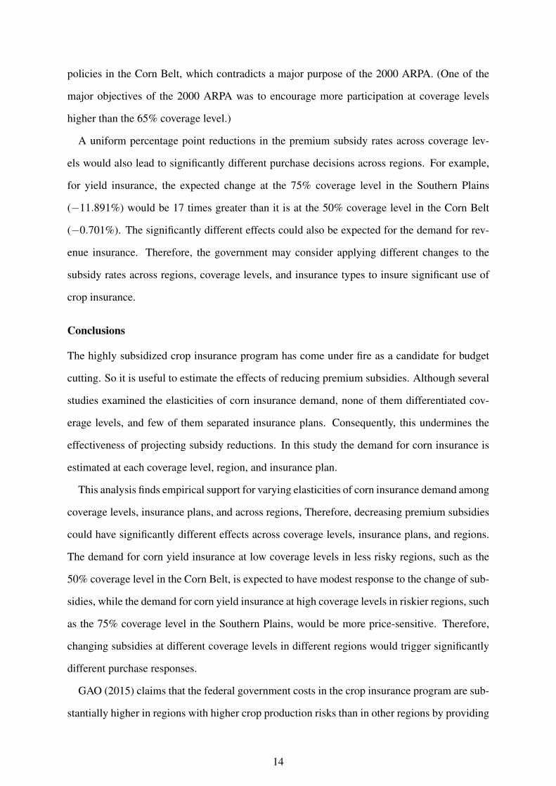
policies in the Corn Belt, which contradicts a major purpose of the 2000 ARPA. (One of the

major objectives of the 2000 ARPA was to encourage more participation at coverage levels

higher than the 65% coverage level.)

A uniform percentage point reductions in the premium subsidy rates across coverage lev-

els would also lead to significantly different purchase decisions across regions. For example,

for yield insurance, the expected change at the 75% coverage level in the Southern Plains

(−11.891%) would be 17 times greater than it is at the 50% coverage level in the Corn Belt

(−0.701%). The significantly different effects could also be expected for the demand for rev-

enue insurance. Therefore, the government may consider applying different changes to the

subsidy rates across regions, coverage levels, and insurance types to insure significant use of

crop insurance.

Conclusions

The highly subsidized crop insurance program has come under fire as a candidate for budget

cutting. So it is useful to estimate the effects of reducing premium subsidies. Although several

studies examined the elasticities of corn insurance demand, none of them differentiated cov-

erage levels, and few of them separated insurance plans. Consequently, this undermines the

effectiveness of projecting subsidy reductions. In this study the demand for corn insurance is

estimated at each coverage level, region, and insurance plan.

This analysis finds empirical support for varying elasticities of corn insurance demand among

coverage levels, insurance plans, and across regions, Therefore, decreasing premium subsidies

could have significantly different effects across coverage levels, insurance plans, and regions.

The demand for corn yield insurance at low coverage levels in less risky regions, such as the

50% coverage level in the Corn Belt, is expected to have modest response to the change of sub-

sidies, while the demand for corn yield insurance at high coverage levels in riskier regions, such

as the 75% coverage level in the Southern Plains, would be more price-sensitive. Therefore,

changing subsidies at different coverage levels in different regions would trigger significantly

different purchase responses.

GAO (2015) claims that the federal government costs in the crop insurance program are sub-

stantially higher in regions with higher crop production risks than in other regions by providing

14

cheaper crop insurance. The cheaper insurance is realized by setting the county base premium

rates much lower than the target premium rates. Although RMA disagrees with GAO’s claim,

it does not have more information to refute GAO’s argument since RMA does not monitor and

report government costs in riskier regions. This study shows that to keep high participation

and high coverage levels, the government premium subsidies would need to be higher in riskier

regions since the demand for corn insurance is more price sensitive in riskier regions and for

higher coverage levels. But how large the differences would be to balance participation and

actuarial fairness between different risk regions deserves more attention and future research.

To estimate the elasticities of demand for corn insurance, this study assumes there is no

adverse selection in the corn insurance market. However, the existence of adverse selection

is one of the longstanding problems in the analysis of crop insurance. The study would be

improved if adverse selection is incorporated in the estimation of demand for corn insurance.

15

Tabl

e6.

Est

imat

edE

last

iciti

esof

Dem

and

for

Cor

nA

PHIn

sura

nce

inth

eC

orn

Bel

t

Var

iabl

e50

%55

%60

%65

%70

%75

%80

%85

%

Net

prem

ium

-0.0

47**

-0.0

28-0

.106

***

-0.1

14**

*-0

.137

***

-0.1

49**

*-0

.230

***

0.01

7

Yie

ldex

pect

atio

n0.

416*

**0.

377*

**0.

347*

**0.

276*

**0.

300*

**0.

534*

**0.

730*

**0.

237

Rel

ativ

eyi

eld

risk

-0.0

80*

-0.0

96-0

.128

*-0

.130

***

-0.0

97*

-0.1

12**

0.03

5-0

.204

*

Plan

ted

acre

s0.

067*

**0.

088*

**0.

050*

**0.

063*

**0.

030*

*0.

021

0.02

90.

100*

**

Enr

olle

dac

res

-0.0

12**

-0.0

24**

*-0

.022

**0.

0004

0.00

40.

01-0

.01

-0.0

22

Perc

enta

geof

irri

gate

dcr

opla

nd-0

.100

-0.1

72-0

.016

0.06

50.

060.

112

-0.1

59-0

.174

Perc

enta

geof

crop

land

oper

ated

byfe

mal

e-0

.148

0.10

50.

095

0.06

4-0

.705

-0.8

430.

075

-0.6

71

Tabl

e7.

Est

imat

edE

last

iciti

esof

Dem

and

for

Cor

nA

PHIn

sura

nce

inth

eL

ake

Stat

es

Var

iabl

e50

%55

%60

%65

%70

%75

%80

%

Net

prem

ium

-0.1

80**

*-0

.138

***

-0.1

38**

*-0

.147

***

-0.0

94**

-0.1

57**

*-0

.158

**

Yie

ldex

pect

atio

n0.

418*

**0.

336*

**0.

644*

**0.

540*

**0.

558*

**0.

756*

**0.

557

Rel

ativ

eyi

eld

risk

-0.0

98**

-0.1

88**

0.05

60.

037

-0.0

310.

019

-0.2

01

Plan

ted

acre

s0.

023*

0.05

5***

0.05

5**

0.04

2***

0.06

8***

0.03

30.

204*

**

Enr

olle

dac

res

inC

RP

-0.0

14**

-0.0

18*

-0.0

20**

-0.0

08*

-0.0

16**

-0.0

02-0

.078

**

Perc

enta

geof

irri

gate

dcr

opla

nd-0

.273

**-0

.121

-0.1

66-0

.022

-0.0

93-0

.031

0.15

6

Perc

enta

geof

crop

land

oper

ated

byfe

mal

e-0

.172

0.41

80.

606

0.30

10.

752

-1.1

713.

709*

*

16

Tabl

e8.

Est

imat

edE

last

iciti

esof

Dem

and

for

Cor

nA

PHIn

sura

nce

inth

eN

orth

ern

Plai

ns

Var

iabl

e50

%55

%60

%65

%70

%75

%80

%85

%

Net

prem

ium

-0.1

70**

*-0

.004

-0.3

05**

*-0

.038

-0.0

97-0

.188

*-0

.259

**-0

.284

**

Yie

ldex

pect

atio

n0.

538*

**0.

724*

**0.

599*

**0.

809*

**0.

720*

**0.

530*

**0.

890*

*-0

.257

*

Rel

ativ

eyi

eld

risk

-0.2

89**

*-0

.257

-0.1

64-0

.137

***

-0.0

57-0

.174

0.08

2-0

.618

***

Plan

ted

acre

s0.

041*

**0.

047

0.05

1**

0.01

5***

0.06

7***

0.07

1***

0.00

2-0

.005

Enr

olle

dac

res

inC

RP

-0.0

18*

-0.0

92**

*0.

0005

-0.0

06-0

.007

-0.0

260.

005

-0.0

41*

Perc

enta

geof

irri

gate

dcr

opla

nd-0

.03

-0.2

38-0

.039

0.05

7-0

.007

-0.0

540.

142

-0.2

37

Perc

enta

geof

crop

land

oper

ated

byfe

mal

e0.

581

0.54

30.

650.

071.

247

1.20

92.

436

1.36

6

Tabl

e9.

Est

imat

edE

last

iciti

esof

Dem

and

for

Cor

nA

PHIn

sura

nce

inth

eSo

uthe

rn

Plai

ns

Var

iabl

e50

%55

%60

%65

%70

%75

%

Net

prem

ium

-0.2

21**

-0.1

31-0

.248

*-0

.227

**-0

.155

-0.6

54**

*

Yie

ldex

pect

atio

n0.

469*

**0.

569*

*0.

455*

*0.

711

0.78

1***

0.85

0***

Rel

ativ

eyi

eld

risk

-0.4

74**

*-0

.026

-0.1

670.

090.

0898

0.00

228

Plan

ted

acre

s-0

.007

140.

0333

-0.0

209

0.00

70.

0012

-0.0

298

Enr

olle

dac

res

inC

RP

0.02

86**

-0.0

047

0.04

02*

0.01

60.

0456

***

0.02

87*

Perc

enta

geof

irri

gate

dcr

opla

nd0.

312*

*0.

634*

*0.

615*

*0.

569*

**0.

525*

*0.

232

Perc

enta

geof

crop

land

oper

ated

byfe

mal

e0.

426

-0.1

21-1

.175

0.01

1.55

3-2

.079

*

17

Tabl

e10

.Est

imat

edE

last

iciti

esof

Dem

and

for

Cor

nC

RC

Insu

ranc

ein

the

Cor

nB

elt

Var

iabl

e50

%55

%60

%65

%70

%75

%80

%85

%

Net

prem

ium

-0.0

150.

033

-0.0

40-0

.083

**-0

.167

***

-0.1

46**

*-0

.200

***

-0.0

83

Rev

enue

expe

ctat

ion

-0.0

88-0

.082

-0.1

94**

*-0

.113

***

-0.1

52**

*-0

.195

***

0.43

2***

0.44

0***

Rel

ativ

ere

venu

eri

sk-0

.009

0.22

6**

0.16

8*-0

.023

0.03

3-0

.020

0.05

1-0

.054

Plan

ted

acre

s0.

148*

**0.

127*

**0.

110*

**0.

108*

**0.

088*

**0.

086*

**0.

009

0.06

1**

Enr

olle

dac

res

inC

RP

-0.0

37**

*-0

.059

***

-0.0

45**

*-0

.022

***

-0.0

17**

*-0

.023

***

-0.0

010.

004

Perc

enta

geof

irri

gate

dcr

opla

nd-0

.204

-0.1

77-0

.109

0.09

90.

004

0.08

0-0

.054

0.09

9

Perc

enta

geof

crop

land

oper

ated

byfe

mal

e1.

239*

-0.0

66-0

.305

-0.9

02*

-1.4

69**

*-0

.572

-1.5

51**

*-1

.635

*

Tabl

e11

.Est

imat

edE

last

iciti

esof

Dem

and

for

Cor

nC

RC

Insu

ranc

ein

the

Lak

eSt

ates

Var

iabl

e50

%55

%60

%65

%70

%75

%80

%85

%

Net

prem

ium

-0.2

13**

*-0

.323

***

-0.1

90**

*-0

.239

***

-0.2

85**

*-0

.229

***

-0.2

08**

*-0

.177

Rev

enue

expe

ctat

ion

-0.1

290.

014

-0.0

050.

031

-0.1

130.

052

1.10

4***

0.36

3

Rel

ativ

ere

venu

eri

sk0.

018

-0.0

230.

295*

*0.

221*

**0.

406*

**0.

334*

**0.

123

-0.0

66

Plan

ted

acre

s0.

120*

**0.

078*

*0.

077*

*0.

105*

**0.

075*

0.03

1-0

.075

0.04

3

Enr

olle

dac

res

inC

RP

-0.0

21*

-0.0

15-0

.037

***

-0.0

19*

-0.0

110.

029*

*0.

040.

014

Perc

enta

geof

irri

gate

dcr

opla

nd-0

.227

-2.0

96**

*-0

.307

-0.1

76-0

.258

**-0

.193

-0.2

380.

029

Perc

enta

geof

crop

land

oper

ated

byfe

mal

e1.

283

3.19

8**

0.67

50.

583

0.21

20.

829

-0.3

08-0

.562

18

Tabl

e12

.Est

imat

edE

last

iciti

esof

Dem

and

for

Cor

nC

RC

Insu

ranc

ein

the

Nor

ther

n

Plai

ns

Var

iabl

e50

%55

%60

%65

%70

%75

%80

%85

%

Net

prem

ium

-0.0

42-0

.205

-0.2

90**

*0.

017

-0.0

440.

097

0.07

50.

009

Rev

enue

expe

ctat

ion

0.07

40.

140.

186*

*0.

236*

**0.

132*

**0.

058

0.83

9***

0.68

6***

Rel

ativ

ere

venu

eri

sk-0

.014

-0.0

110.

046

-0.1

29**

0.00

6-0

.025

0.06

1-0

.108

Plan

ted

acre

s0.

024

0.03

90.

035

0.04

9***

0.01

0.06

1***

0.06

9***

-0.0

04

Enr

olle

dac

res

inC

RP

0.00

20.

011

0.01

4-0

.020

**0.

020*

*0.

001

0.00

20.

020

Perc

enta

geof

irri

gate

dcr

opla

nd0.

491*

**0.

241

0.34

8***

0.26

3***

0.48

0***

0.50

3***

-0.0

310.

176

Perc

enta

geof

crop

land

oper

ated

byfe

mal

e0.

314

0.04

32.

140*

0.92

3*0.

588

2.40

6***

1.04

5-3

.308

**

Tabl

e13

.Est

imat

edE

last

iciti

esof

Dem

and

for

Cor

nC

RC

Insu

ranc

ein

the

Sout

hern

Plai

ns

Var

iabl

e50

%55

%60

%65

%70

%75

%

Net

prem

ium

-0.3

31**

-0.0

94-0

.373

***

-0.2

42*

-0.5

01**

*-0

.670

***

Rev

enue

expe

ctat

ion

0.33

3***

0.56

4***

0.79

7***

0.51

9***

0.81

9***

0.61

3**

Rel

ativ

ere

venu

eri

sk0.

229*

-0.0

67-0

.005

0.16

0**

-0.1

71*

0.02

3

Plan

ted

acre

s0.

074*

*0.

050

0.02

10.

080*

**-0

.008

-0.0

21

Enr

olle

dac

res

inC

RP

0.07

2***

0.06

80.

036*

*0.

041*

**0.

021

0.05

3**

Perc

enta

geof

irri

gate

dcr

opla

nd0.

741*

**0.

738*

0.36

1*0.

471*

**0.

669*

**0.

364

Perc

enta

geof

crop

land

oper

ated

byfe

mal

e-0

.031

-3.4

353.

341*

*3.

776*

**1.

629

2.84

4*

19

References

Babcock, B.A., and C.E. Hart. 2005. “Influence of the premium subsidy on farmers’ crop in-

surance coverage decisions.”, pp. .

Babcock, B.A., C.E. Hart, and D.J. Hayes. 2004. “Actuarial fairness of crop insurance rates

with constant rate relativities.” American Journal of Agricultural Economics 86:563–575.

Bruin, J. 2006. “Newtest: command to compute new test. UCLA: Statistical Consulting Group.”

Cannon, D., and B. Barnett. 1995. “Modeling changes in participation in the federal Multiple

Peril Crop Insurance program between 1982 and 1987.” American Journal of Agricultural

Economics 77:1380–1380.

Charness, G., and U. Gneezy. 2012. “Strong evidence for gender differences in risk taking.”

Journal of Economic Behavior & Organization 83:50–58.

Coble, K.H., and B.J. Barnett. 2013. “Why do we subsidize crop insurance?” American Journal

of Agricultural Economics 95:498–504.

Gardner, B.L., and R.A. Kramer. 1986. “Experience with crop insurance programs in the United

States.”, pp. .

Glauber, J.W. 2004. “Crop insurance reconsidered.” American Journal of Agricultural Eco-

nomics 86:1179–1195.

Goodwin, B.K. 1993. “An empirical analysis of the demand for multiple peril crop insurance.”

American Journal of Agricultural Economics 75:425–434.

—. 2001. “Problems with market insurance in agriculture.” American Journal of Agricultural

Economics 83:643–649.

Goodwin, B.K., and A.P. Ker. 1998. “Nonparametric estimation of crop yield distributions: im-

plications for rating group-risk crop insurance contracts.” American Journal of Agricultural

Economics 80:139–153.

Goodwin, B.K., M.L. Vandeveer, and J.L. Deal. 2004. “An empirical analysis of acreage effects

of participation in the federal crop insurance program.” American Journal of Agricultural

Economics 86:1058–1077.

Kelley, C.R. 2001. “Agricultural Risk Protection Act of 2000: Federal Crop Insurance, the

Non-Insured Crop Disaster Assistance Program, and the Domestic Commodity and Other

20

Farm Programs, The.” Drake J. Agric. L. 6:141.

Knox, L., and T.J. Richards. 1999. “A two-stage model of the demand for specialty crop insur-

ance.” In American Agricultural Economics Association, Summer Meeting. Nashville, Ten-

nessee.

O’Donoghue, E. 2014. “The Effects of Premium Subsidies on Demand for Crop Insurance.”

USDA-ERS Economic Research Report, pp. .

Richards, T.J. 2000. “A two-stage model of the demand for specialty crop insurance.” Journal

of agricultural and resource economics, pp. 177–194.

Serra, T., B.K. Goodwin, and A.M. Featherstone. 2003. “Modeling Changes in the US Demand

for Crop Insurance during the 1990s.” Agricultural Finance Review 63:109–125.

Shields, D.A. 2015. “Federal Crop Insurance: Background.” Congressional Research Service,

pp. .

Smith, V.H., and A.E. Baquet. 1996. “The demand for multiple peril crop insurance: evidence

from Montana wheat farms.” American journal of agricultural economics 78:189–201.

Wang, H.H., S.D. Hanson, R.J. Myers, and J.R. Black. 1998. “The effects of crop yield insur-

ance designs on farmer participation and welfare.” American Journal of Agricultural Eco-

nomics 80:806–820.

21