Board of Governors of the Federal Reserve System

International Finance Discussion Papers

Number 1048

May 2012

How Do Laffer Curves Differ Across Countries?

Mathias Trabandt

and

Harald Uhlig NOTE: International Finance Discussion Papers are preliminary materials circulated to stimulate discussion and critical comment. References to International Finance Discussion Papers (other than an acknowledgment that the writer has had access to unpublished material) should be cleared with the author or authors. Recent IFDPs are available on the Web at www.federalreserve.gov/pubs/ifdp/. This paper can be downloaded without charge from the Social Science Research Network electronic library at www.ssrn.com.

How Do Laffer Curves Differ Across Countries?I

Mathias Trabandta, Harald Uhligb,c

aMathias Trabandt, Board of Governors of the Federal Reserve System, 20th Street and Constitution AvenueN.W., Washington, D.C. 20551, USA

bHarald Uhlig, Department of Economics, University of Chicago, 1126 East 59th Street, Chicago, IL 60637, USA

cNBER, CEPR, CentER, Deutsche Bundesbank

Abstract

We seek to understand how Laffer curves differ across countries in the US and the EU-14, thereby

providing insights into fiscal limits for government spending and the service of sovereign debt.

As an application, we analyze the consequences for the permanent sustainability of current debt

levels, when interest rates are permanently increased e.g. due to default fears. We build on the

analysis in Trabandt and Uhlig (2011) and extend it in several ways. To obtain a better fit to

the data, we allow for monopolistic competition as well as partial taxation of pure profit income.

We update the sample to 2010, thereby including recent increases in government spending and

their fiscal consequences. We provide new tax rate data. We conduct an analysis for the pes-

simistic case that the recent fiscal shifts are permanent. We include a cross-country analysis

on consumption taxes as well as a more detailed investigation of the inclusion of human capital

considerations for labor taxation.

Keywords: Laffer curve, taxation, cross country comparison, debt sustainability, fiscal limits,

quantitative endogenous growth, human capital and labor taxation

JEL Classification: E0, E13, E2, E3, E62, H0, H2, H3, H6

IThis version: May 4, 2012. We are grateful to Roel Beetsma and Jaume Ventura for useful discussions.Further, we are grateful to Alan Auerbach, Alberto Alesina, Axel Boersch-Supan, Francesco Giavazzi, LaurenceKotlikoff and Valerie Ramey for useful comments and suggestions. The views expressed in this paper are solelythe responsibility of the authors and should not be interpreted as reflecting the views of the Board of Governorsof the Federal Reserve System or of any other person associated with the Federal Reserve System.

Email addresses: mathias.trabandt@gmail.com (Mathias Trabandt), huhlig@uchicago.edu (HaraldUhlig)

1. Introduction

We seek to understand how Laffer curves differ across countries in the US and the EU-14. This

provides insight into the limits of taxation. As an application, we analyze the consequences of

recent increases in government spending and their fiscal consequences as well as the consequences

for the permanent sustainability of current debt levels, when interest rates are permanently high

e.g. due to default fears.

We build on the analysis in Trabandt and Uhlig (2011). There, we have characterized Laffer

curves for labor and capital taxation for the U.S., the EU-14, and individual European coun-

tries. In the analysis, a neoclassical growth model featuring “constant Frisch elasticity” (CFE)

preferences are introduced and analyzed: we use the same preferences here. The results there

suggest that the U.S. could increase tax revenues considerably more than the EU-14, and that

conversely the degree of self-financing of tax cuts is much larger in the EU-14 than in the U.S.

While we have calculated results for individual European countries, the focus there was directed

towards a comparison of the U.S. and the aggregate EU-14 economy.

This paper provides a more in-depth analysis of the cross-country comparison. Furthermore,

we modify the analysis in two important dimensions. The model in Trabandt and Uhlig (2011)

overstates total tax revenues to GDP compared to the data: in particular, labor tax revenues

to GDP are too high. We introduce monopolistic competition to solve this: capital income now

consists out of rental rates to capital as well as pure profits, decreasing the share of labor income

in the economy. With this change alone, the model now overpredicts the capital income tax

revenue. We therefore furthermore assume that only a fraction of pure profit income is actually

reported to the tax authorities and therefore taxed. With these two changes, the fit to the data

improves compared to the original version, see figure 2. In terms of the Laffer curves, this moves

countries somewhat closer to the peak of the labor tax Laffer curve and somewhat farther away

from the peak of the capital tax Laffer curve. For the cross-country comparison, we assume

that all structural parameters for technologies and preferences are the same across countries.

The differences between the Laffer curves therefore arise solely due to differences in fiscal policy

i.e. the mix of distortionary taxes, government spending and government debt. We find that

2

labor income and consumption taxes are important for accounting for most of the cross-country

differences.

We refine the methodology of Mendoza et al. (1994) to calculate effective tax rates on labor and

capital income. Broadly, we expand the measured labor tax base by including supplements to

wages as well as a fraction of entrepreneurial income of households. As a result, the refinements

imply a more reasonable labor share in line with the literature. More importantly, the average

1995-2010 labor income taxes turn out to be lower while capital income taxes are somewhat

higher as previously calculated in Trabandt and Uhlig (2011).

We update our analysis in Trabandt and Uhlig (2011) by including the additional years 2008-

2010. This is particularly interesting, as it allows us to examine the implications of the recent

substantial tax and revenue shocks. While recent fiscal policy changes were intended to be

temporary, we examine the pessimistic scenario that they are permanent. To do so, we calibrate

the model to the Laffer curves implied by the strained fiscal situation of 2010, and compare them

to the Laffer curves of the average extended sample 1995-2010. We find that the 2010 calibration

moves almost all countries closer to the peak of the labor tax Laffer curve, with the scope for

additional labor tax increases cut by a third for most countries and by up to one half for some

countries. It is important, however, to keep the general equilibrium repercussions of raising taxes

in mind: even though tax revenues may be increased by some limited amount, tax bases and

thereby output fall when moving to the peak of the Laffer curve due to the negative incentive

effects of higher taxes.

We then use these results to examine the scope for long-term sustainability of current debt levels,

when interest rates are permanently higher due to, say, default fears. This helps to understand

the more complex situation of an extended period with substantially increased interest rates due

to, say, default fears. More precisely, we answer the following question: what is the maximum

steady state interest rate on outstanding government debt that the government could afford

without cutting government spending, based on a calibration to the fiscal situation in 2010? To

do so, we calculate the implied peak of the Laffer curve and compute the maximum interest

rate on outstanding government debt in 2010 that would still balance the government budget

constraint in steady state. The results of our baseline model are in table 7: the most interesting

3

column there may be the second one. We find that the USA can afford the highest interest rate

if labor taxes are moved to the peak of the Laffer curve: depending on the debt measure used, a

real interest rate of of 12% to 15.5% is sustainable. Interestingly, Ireland can also afford the high

rate of 11.2%, when moving labor taxes only. By contrast, Austria, Belgium, Denmark, Finland,

France, Greece and Italy can only afford permanent real rates in the range of 4.4% to 7.1%, when

financing the additional interest payments with higher labor tax rates alone, while, say, Germany,

Portugal and Spain can all afford an interest rate somewhere above 9%. The picture improves

somewhat, but not much, when labor taxes and capital taxes can both be adjusted: notably,

Belgium, Denmark, Finland, France and Italy cannot permanently afford real interest rates above

6.5%. Below we also examine the implications of human capital accumulation and show that the

maximum interest rates may be even lower than suggested by our baseline model. It is worth

emphasizing that we have not included the possibility of cutting government spending and/or

transfers and that our analysis has focussed on the most pessimistic scenario of a permanent

shift.

In the baseline model, physical capital is the production factor that gets accumulated. It may

be important, however, to allow for and consider human capital accumulation, when examining

the consequences of changing labor taxation. We build on the quantitative endogenous growth

models introduced in Trabandt and Uhlig (2011), and provide a more detailed cross-country com-

parison. We find that the capital tax Laffer curve is affected only rather little across countries

when human capital is introduced into the model. By contrast, the introduction of human capital

has important effects for the labor income tax Laffer curve. Several countries are pushed on the

slippery slope sides of their labor tax Laffer curves once human capital is accounted for. Intu-

itively, higher labor taxes lead to a faster reduction of the labor tax base since households work

less and aquire less human capital which in turn leads to lower labor income. We recalculate the

implied maximum interest rates on government debt in 2010 when human capital accumulation

is allowed for in the model. Table 9 contains the results: the US may only afford a real interest

rate between 5.8% to 6.6% in this case. Most of the European countries cluster between 4% and

4.9% except for Denmark, Finland and Ireland who can afford real interest rates between 5.9%

and 9.5%.

4

We add a cross-country analysis on consumption taxes. In Trabandt and Uhlig (2011), we have

shown that the consumption tax Laffer curve has no peak. Essentially, the difference between the

labor tax Laffer curve and the consumption tax Laffer curve arises due to “accounting” reasons:

the additional revenues are provided as transfers, and are used for consumption purchases, to be

taxed at the consumption tax rate. In Trabandt and Uhlig (2011), we only provided the analysis

for the U.S. and the aggregate EU-14 economy. Here, we extend the consumption tax analysis

to individual countries. The range of maximum additional tax revenues (in percent of GDP) in

the baseline model is roughly 40-100 percent while it shrinks to roughly 10-30 percent in the

model with added human capital. Higher consumption taxes affect equilibrium labor via the

labor wedge, similar to labor taxes. As above, human capital amplifies the reduction of the labor

tax base triggered by the change in the labor wedge. Overall, maximum possible tax revenues

due to consumption taxes are reduced massively, although at fairly high consumption tax rates.

The paper is organized as follows. Section 2 provides the model. The calibration and parame-

terization of the model can be found in section 3. Section 4 provides and discusses the results.

Section 5 discusses the extension of the model with human capital as well as the results for

consumption taxation. Finally, section 6 concludes.

2. Model

We employ the baseline model in Trabandt and Uhlig (2011) and extend it by allowing for inter-

mediate inputs, supplied by monopolistically competitive firms. Time is discrete, t = 0, 1, . . . ,∞.

Households maximize

maxct,nt,kt,xt,bt E0

∞∑t=0

βt [u(ct, nt) + v(gt)]

subject to

(1 + τ ct )ct + xt + bt = (1− τnt )wtnt + (1− τ kt )[(dt − δ)kt−1 + ϕΠt]

+δkt−1 +Rbtbt−1 + st + (1− ϕ)Πt +mt

kt = (1− δ)kt−1 + xt (1)

5

where ct, nt, kt, xt, bt, mt denote consumption, hours worked, capital, investment, government

bonds and an exogenous stream of payments. The household takes government consumption

gt, which provides utility, as given. Further, the household receives wages wt, dividends dt,

profits Πt from firms and asset payments mt. The payments mt are a stand-in for net imports,

modelled here as exogenously given income from a “tree”, see Trabandt and Uhlig (2011) for

further discussion. The household obtains interest earnings Rbt and lump-sum transfers st from

the government. It has to pay consumption taxes τ ct , labor income taxes τnt and capital income

taxes τ kt on dividends and on a share ϕ of profits.1

As introduced and extensively discussed in Trabandt and Uhlig (2011), but also used in Hall

(2009), Shimer (2009) and King and Rebelo (1999), we work with constant Frisch elasticity

preferences (CFE), given by

u(c, n) = log(c)− κn1+ 1φ (2)

if η = 1, and by

u(c, n) =1

1− η

(c1−η

(1− κ(1− η)n1+ 1

φ

)η

− 1)

(3)

if η > 0, η = 1, where κ > 0. These preferences are consistent with balanced growth and feature

a constant Frisch elasticity of labor supply, given by φ, without constraining the intertemporal

elasticity of substitution.

Competitive final good firms maximize profits

maxkt−1,zt yt − dtkt−1 − ptzt (4)

subject to the Cobb-Douglas production technology, yt = ξtkθt−1z1−θt , where ξt denotes the trend

of total factor productivity. pt denotes the price of an homogenous input, zt, which in turn is

produced by competitive firms who maximize profits

maxzt,i

ptzt −∫pt,izt,idi (5)

1We allow for partial profit taxation due to the various deductions and exemptions that are available for firmsand households in this regard. Further, note that capital income taxes are levied on dividends net-of-depreciationas in Prescott (2002, 2004) and in line with Mendoza et al. (1994).

6

subject to zt =(∫

z1ωt,i di

)ω

with ω > 1. Intermediate inputs, zt,i, are produced by monopolisti-

cally competitive firms which maximize profits

maxpt,i

pt,izt,i − wtnt,i

subject to their demand functions and production technologies:

zt,i =

(ptpt,i

) ωω−1

zt

zt,i = nt,i

In equilibrium, all firms set the same price which is a markup over marginal costs. Formally,

pt,i = pt = ωwt. Aggregate equilibrium profits are given by Πt = (ω − 1)wtnt.

The government faces the budget constraint,

gt + st +Rbtbt−1 = bt + Tt (6)

where government tax revenues are given by

Tt = τ ct ct + τnt wtnt + τ kt [(dt − δ)kt−1 + ϕΠt] (7)

It is the goal to analyze how the equilibrium shifts, as tax rates are shifted. More generally,

the tax rates may be interpreted as wedges as in Chari et al. (2007), and some of the results

in this paper carry over to that more general interpretation. What is special to the tax rate

interpretation and crucial to the analysis in this paper, however, is the link between tax receipts

and transfers (or government spending) via the government budget constraint.

The paper focuses on the comparison of balanced growth paths. We assume that government

debt, government spending as well as net imports do not deviate from their balanced growth

paths, i.e. we assume that bt−1 = ψtb, gt = ψtg as well as mt = ψtm where ψ is the growth

factor of aggregate output. We consider exogenously imposed shifts in tax rates or in returns

7

on government debt. We assume that government transfers adjust according to the government

budget constraint (6), rewritten as st = ψtb(ψ −Rbt) + Tt − ψtg.

2.1 Equilibrium

In equilibrium the household chooses plans to maximize its utility, the firm solves its maximiza-

tion problem and the government sets policies that satisfy its budget constraint. In what follows,

key balanced growth relationships of the model that are necessary for computing Laffer curves

are summarized. Except for hours worked, interest rates and taxes all other variables grow at a

constant rate ψ = ξ1

1−θ . For CFE preferences, the balanced growth after-tax return on any asset

is R = ψη/β. It is assumed throughout that ξ ≥ 1 and that parameters are such that R > 1,

but β is not necessarily restricted to be less than one. Let k/y denote the balanced growth path

value of the capital-output ratio kt−1/yt. In the model, it is given by

k/y =

(R− 1

θ(1− τ k)+δ

θ

)−1

. (8)

Labor productivity and the before-tax wage level are given by,

ytn

= ψt k/yθ

1−θ and wt =(1− θ)

ω

ytn.

It remains to solve for the level of equilibrium labor. Let c/y denote the balanced growth path

ratio ct/yt. With the CFE preference specification and along the balanced growth path, the

first-order conditions of the household and the firm imply

(ηκn1+ 1

φ

)−1

+ 1− 1

η= α c/y (9)

where α = ω(1+τc

1−τn

)(1+ 1φ

1−θ

)depends on tax rates, the labor share, the Frisch elasticity of labor

supply and the markup.

8

In this paper, we shall concentrate on the case when transfers s are varied and government

spending g is fixed. Then, the feasibility constraint implies

c/y = χ+ γ1

n(10)

where χ = 1 − (ψ − 1 + δ) k/y and γ = (m− g) k/y−θ1−θ . Substituting equation (10) into (9)

therefore yields a one-dimensional nonlinear equation in n, which can be solved numerically,

given values for preference parameters, production parameters, tax rates and the levels of b, g

and m.

After some straightforward algebra, total tax revenues along a balanced growth path can be

calculated as

T =

[τ cc/y + τn

(1− θ)

ω+ τ k

(θ − δk/y + ϕ(1− θ)

ω − 1

ω

)]y (11)

and equilibrium transfers are given by,

s =(ψ −Rb

)b− g + T . (12)

3 Data, calibration and parameterization

The model is calibrated to annual post-war data of the USA, the aggregate EU-14 economy and

individual European countries. An overview of the calibration is in tables 1 and 2.

We refine the methodology of Mendoza et al. (1994) to calculate effective tax rates on labor and

capital income. Broadly, we expand the measured labor tax base by including supplements to

wages as well as a fraction of entrepreneurial income of households. As a result, the refinements

imply a more reasonable labor share in line with the empirical literature. More importantly, the

average 1995-2010 labor income taxes turn out to be lower while capital income taxes are higher

as previously calculated in Trabandt and Uhlig (2011). Appendix A provides the new tax rates

across countries over time and Appendix B contains the details on the calculations with further

discussion of the implications for e.g. the Laffer curves.

9

There are two new key parameters, compared to Trabandt and Uhlig (2011). The first parameter

is ω, the gross markup, due to monopolistic competition. We set ω = 1.1, which appears to be a

reasonable number, given the literature. The second parameter is ϕ, the share of monopolistic-

competition profits which are subject to capital taxes. We set this parameter equal to the capital

share, i.e. to 0.36. While we could have explored specific evidence to help us pin down this

parameter, we have chosen this value rather arbitrarily and with an eye towards the fit of the

model to the data instead.

The sample covered in Trabandt and Uhlig (2011) is 1995-2007. Here we extend the sample

to 2010 using the same data sources. We update all data up to 2010, except for taxes and

tax revenues which we can update only to 2009 due to data availability reasons. For most of

the analysis in this paper, we assume that the 2010 observation for taxes and revenues are the

same as in 2009. We also pursue an alternative approach for tax rates for the year 2010, see

subsection 3.2 below for the details.

We also refine the calculation of transfers in the data compared to Trabandt and Uhlig (2011).

In the data, there is a non-neglible difference between government tax revenues and government

revenues. This difference is mostly due to “other government revenue” and “government sales”.

We substract these two items from the measure of transfers defined in Trabandt and Uhlig (2011).

US and aggregate EU-14 tax rates, government expenditures and government debt are set accord-

ing to the upper part of table 1. We also calibrate the model to individual EU-14 country data

for tax rates, government spending and government debt as provided in table 2. Although we

allow fiscal policy to be different across countries, we restrict the analysis to identical parameters

across countries for preferences and technology, see the lower part of table 1 for the details.2

Finally, the empirical measure of government debt for the US as well as the EU-14 area provided

by the AMECO database is nominal general government consolidated gross debt (excessive deficit

procedure, based on ESA 1995) which is divided by nominal GDP. For the US the gross debt to

GDP ratio is 66.2% in the sample. For checking purposes, we also examine the implications if

2See Trabandt and Uhlig (2011) for the differences with respect to Laffer curves when parameters for technologyand preferences are assumed to be identical or country specific.

10

we use an alternative measure of US government debt: debt held by the public. See tables 1 and

2 for the differences. However, given that to our knowledge data on “debt held by the public”

is not available for European countries, we shall proceed by using gross debt as a benchmark if

not otherwise noted. Where appropriate, we shall perform a sensitivity analysis with respect to

the measure of US government debt.

3.1 Model Fit and Sensitivity

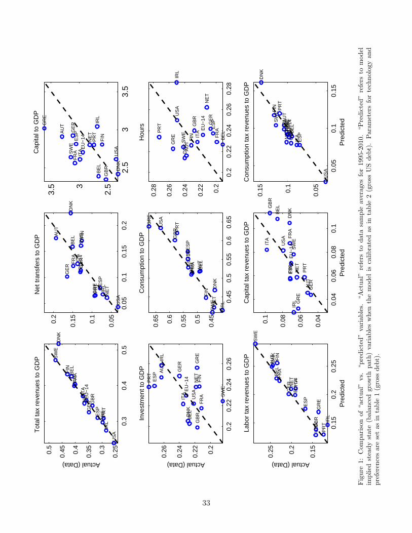
The structual parameters are set such that model implied steady states are close to the data. In

particular, figure 1 provides a comparison of the data vs. model fit for key great ratios, hours

as well as transfers and tax revenues.3 Overall, the fit is remarkable given the relatively simple

model in which country differences are entirely due to fiscal policy.4

Most of the structual parameter values in the lower part of table 1 are standard and perhaps

uncontroversial, see e.g. Cooley and Prescott (1995), Prescott (2002, 2004, 2006) and Kimball

and Shapiro (2008).

The new parameters here compared to Trabandt and Uhlig (2011) are the gross markup, ω = 1.1

and the share of monopolistic-competition profits subject to capital taxation, ϕ = θ = 0.36.

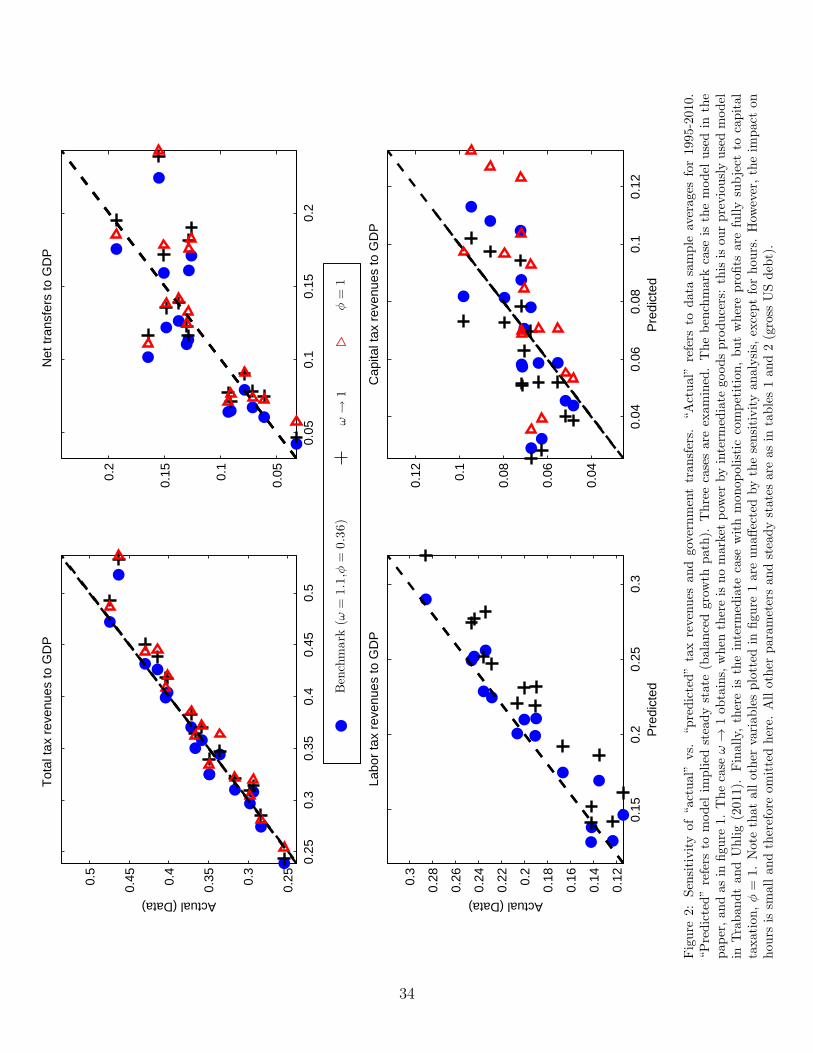
Figure 2 contains a sensitivity analysis for ω and ϕ. When ω → 1, the model overstates labor tax

revenues and understates capital tax revenues, see the black crosses in figure 2.5 In the adapted

model with intermediate inputs, a gross markup ω > 1 reduces the labor tax base. At the same

time, profits increase the capital tax base, but too much if profits are fully subject to capital

taxation, i.e. ϕ = 1, see the red triangles in figure 2. Overall, the fit improves considerably if we

set the share of profits subject to capital taxes, ϕ = θ = 0.36. The fit is not sensitive to ϕ: all

values in ϕ ∈ [0.3, 0.4] work practically just as well in terms of the fit, for example.

3We assume a mapping of data and model in the literal sense, i.e. the one based on the definitions of thenational income and product accounts and the revenues statistics. For work that takes an alternative perspectiveand emphasizes the general relativity of fiscal language, see Green and Kotlikoff (2009).

4The present paper, and in particular the comparison of data vs. model hours is closely related to Prescott(2002, 2004) and subsequent contributions by e.g. Blanchard (2004), Alesina et al. (2006), Ljungqvist and Sargent(2007), Rogerson (2007) and Pissarides and Ngai (2009).

5Note that in this case, the value of ϕ becomes immaterial since equilibrium profits are zero.

11

3.2. The year 2010

At the end of our sample, government spending and government debt have risen substantially

as a fallout of the financial crisis, see table 2. We are particularly interested in characterizing

Laffer curves for the year 2010. While there is no tax rate data for the year 2010 at the time

of writing this paper, we do have data for government spending and debt in 2010. We wish to

consider the pessimistic scenario of a steady state, in which these changes are permanent. We

therefore use the government budget constraint of the model to infer the labor tax rate, i.e. we

calculate the implied labor tax given government debt and government consumption in 2010 as

well as average (1995-2010) model implied government transfers.

Table 2 contains the resulting labor tax rates across countries. According to the model, in the

US and EU-14 labor taxes need to be 5-8 percentage points higher to balance the government

budget in 2010 compared to the sample average. There is substantial country specific variation.

While e.g. labor taxes in Germany and Italy remain unchanged, those in the United Kingdom,

Ireland, Spain and the Netherlands increase by 10 or more percentage points.

4. Results

4.1. Sources of differences of Laffer curves

What accounts for the differences between the USA Laffer curves and (individual) EU-14 Laffer

curves? To answer this question, we proceed as follows. As before, we calibrate the model to

country specific averages of 1995-2010, see table 2, keeping structural parameters as in table 1.

Next, we compute Laffer curves.

Results are in the “Baseline” column of tables 3 and 4. All other columns report results if in

the USA calibration, fiscal instruments are set to European country specific values, one at a

time. It appears that labor income and consumption taxes are most important for accounting

for cross-country differences.

Imposing country specific debt to GDP ratios has no effect in our calculations, due to Ricardian

equivalence: a different debt to GDP ratio, holding taxes and government consumption fixed,

results in different transfers along the equilibrium path.

12

Finally, note that compared to Trabandt and Uhlig (2011), intermediate inputs and profit tax-

ation in the present paper move countries somewhat closer to the peak of the labor tax Laffer

curve and somewhat farther away from the peak of the capital tax Laffer curve.

4.2. Laffer curves: average 1995-2010 vs. 2010

To compute Laffer curves, we trace out tax revenues across balanced growth paths, as we change

either labor tax rates or capital tax rates, and computing the resulting changes in transfers. When

changing both tax rates, we obtain a “Laffer hill”. We compute Laffer curves and the Laffer hill

for a 1995-2010 vs. 2010 calibration, i.e., when the model is calibrated in terms of fiscal policy

either to the average of 1995-2010 or to the year 2010, see table 2. Structural parameters are set

as in table 1.

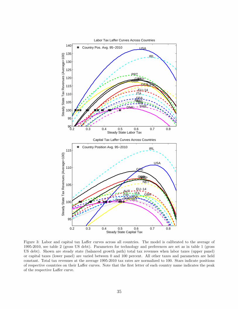
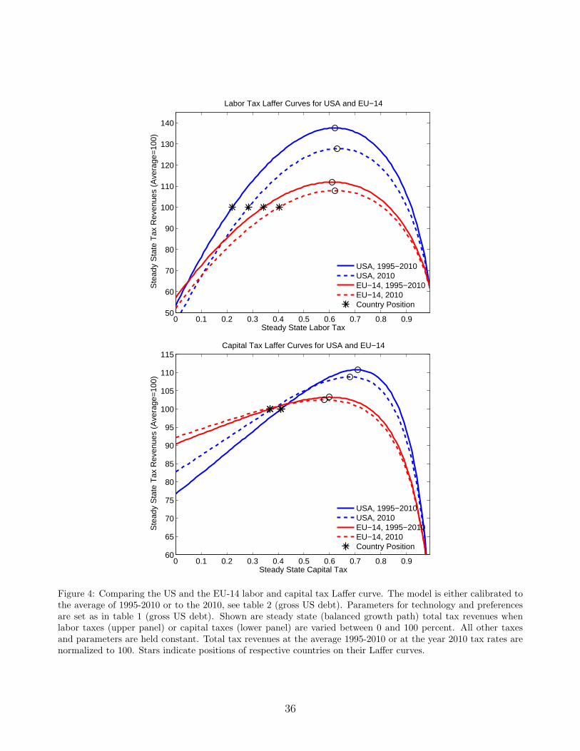
Figure 3 shows the resulting Laffer curves for all countries for the average 1995-2010 calibration.

Figure 4 provides a comparison of Laffer curves for the 1995-2010 vs. 2010 calibration for the

USA and aggregate EU-14 economy. Further cross-country results in this respect are available in

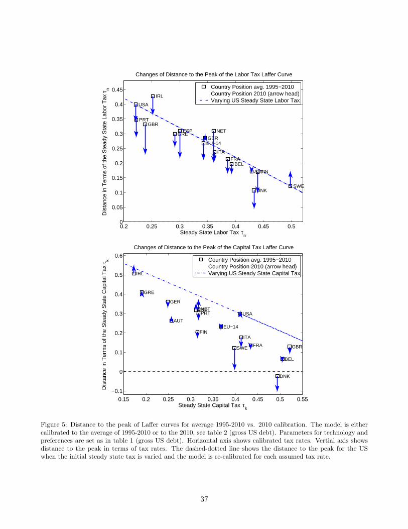
table 5 and in figure 5. The latter figure shows how far each country is from its peak, given its

own tax rate: perhaps not surprisingly, the points line up pretty well. In the figure, we compare

it to the benchmark of performing the same calculation for the US, given by the dash-dotted

line: there, we change, say, the labor tax rate, and, for each new labor tax rate, recalculate κ as

well as g, m and b to obtain the same n and g/y, b/y and m/y as in table 1. We then recalculate

s and s/y to balance the government budget and calculate the distance to the peak of the Laffer

curve. One would expect this exercise to result in a line with a slope close to -1, and indeed,

this is what the figure shows. The points for the individual countries line up close to this line,

though not perfectly: in particular, for the capital tax rate, the distance can be considerable,

and is largely explained by the cross-country variation in labor taxes and consumption taxes.

According to the results, the vast majority of countries have moved closer to the peaks of their

labor and capital income tax Laffer curves and Laffer hills respectively. The movements to the

peaks are sizeable for some countries such as e.g. the United Kingdom, the Netherlands and

Ireland for labor taxes. As above and for the average 1995-2010 sample, it does not matter

13

whether “gross US debt or “US debt held by the public” is used. For the year 2010, however,

small differences arise since transfers are kept at the model average for 1995-2010.

Finally, table 6 provides the output losses associated with moving to the peak of the Laffer curve.

According to the model, US and EU-14 output falls by about 27 respectively 14 percent when

labor taxes are moved to the peak of the Laffer curve. The magnitudes for the case of capital

taxes are similar. There is considerable country specific variation among European countries:

Denmark looses 4 percent while Ireland looses 24 percent of output at the labor tax Laffer curve

peak. Clearly, if a country is already close to its Laffer curve peak in terms of tax rates, the

output losses associated with increasing taxes a little more to attain the peak are more muted

than in a country that has more scope to increase tax revenues. Nevertheless, the table highlights

the general equilibrium repercussions of raising taxes: even though tax revenues may be increased

by some limited amount, tax bases and thereby output fall when moving to the peak of the Laffer

curve due to the negative incentive effects of higher taxes.

4.3. Laffer curve and interest rates

What is the maximum interest rate on outstanding government debt that the government could

afford without cutting government spending? Put differently, how high can interest rates on

government debt be due to, say, default fears (and not due to generally higher discounting by

households), so that fiscal sustainability is still preserved if countries move to the peak of their

Laffer curves?

To answer this question we pursue the following experiment. We calibrate the model in terms of

fiscal policy to the year 2010, see table 2. Structual parameters are set as in table 1. We calculate

Laffer curves for labor and capital taxation as well as the Laffer hill for joint variations of capital

and labor taxes. Keeping model implied government transfers and government consumption

to GDP ratios at their 2010 levels, we calcuate the interest rate that balances the government

budget at maximal tax revenues.

For the calcuations, we focus on balanced growth relationships ignoring transition issues for

simplicity. Consider the scaled government budget constraint along the balanced growth path:

14

(s/y

)2010

+(g/y

)2010

=(b/y

)2010

(ψ − RMax) +(T/y

)Max

(13)

where(T/y

)Max

denotes the maximum additional tax revenues (expressed in % of baseline GDP)

that results from moving from the 2010 status quo to the peak of the Laffer curve. We solve for

RMax = 1 + rMax that balances the above government budget constraint.

Table 7 contains the baseline model results. For each of the three tax experiments (adjusting only

labor taxes, adjusting only capital taxes, adjusting both), the table lists the maximal additional

obtainable revenue as a share of GDP as well as the maximal sustainable interest rate that can be

sustained with these revenues. For comparison, the last two columns of the table also contain real

long-term interest rates for 2010 downloaded from the European Commission AMECO database.

These are nominal 10 years government bond interest rates minus inflation - either using the GDP

deflator (ILRV, first column) or the consumption deflator (ILRC, second column). The value for

the aggregate EU-14 is the real GDP weighted average of individual European countries.

The most interesting column in table 7 may be the second one. We find that the USA can afford

the highest interest rate if labor taxes are moved to the peak of the Laffer curve: depending on the

debt measure used, a real interest rate of of 12% to 15.5% is sustainable. Interestingly, Ireland can

also afford the high rate of 11.2%, when moving labor taxes only. By contrast, Austria, Belgium,

Denmark, Finland, France, Greece and Italy can only afford permanent real rates in the range of

4.4% to 7.1%, when financing the additional interest payments with higher labor tax rates alone,

while, say, Germany, Portugal and Spain can all afford an interest rate somewhere above 9%.

The picture improves somewhat, but not much, when labor taxes and capital taxes can both be

adjusted: notably, Belgium, Denmark, Finland, France and Italy cannot permanently afford real

interest rates above 6.5%.

Note that now, the comparison of “US gross government debt” vs. “US debt held by the public”

matters for the results since government spending is kept constant. Indeed, the US could affort

higher interest rates if “US debt held by the public” is considered.

15

Interestingly, in the next section, we also examine the implications of human capital accumulation

and show that the maximum interest rates may be even lower than suggested by our baseline

model.

For the above analysis, some caveats should be kept in mind. The interest rate on outstand-

ing government debt deviates from the one on private capital but does not crowd out private

investment. In other words, it is implicitly assumed that the interest rate payments due to the

higher interest rate are paid lump-sum to the households and thereby do not affect household

consumption, hours or investment, and that it does not affect the rate at which firms can borrow

privately.6

Note that the steady state safe real interest rate is calibrated to equal 4 percent and represents

therefore the lower bound for rMax: our analysis on sustainable rates may therefore be too

optimistic, keeping in mind that the interest rates are real interest rates, not nominal interest

rates. It is worth emphasizing that we have not included the possibility of cutting government

spending and/or transfers and that our analysis has focussed on the most pessimistic scenario of

a permanent shift.

5. Extensions: human capital, consumption taxes

5.1. Baseline model vs. human capital accumulation

We compare the distance to the peak of Laffer curves for the above baseline model and the

above baseline model with added human capital accumulation. More specifically, we assume

that human capital is accumulated following the second generation case considered in Trabandt

and Uhlig (2011).7

6For related work, see e.g. Bi (2010) and Bi et al. (2010).7See e.g. Jones (2001), Barro and i Martin (2003) or Acemoglu (2008) for textbook treatments of models with

endogenous growth and human capital accumulation. Below we consider a specification incorporating learning-by-doing as well as schooling, following Lucas (1988) and Uzawa (1965). While first-generation endogenous growthmodels have stressed the endogeneity of the overall long-run growth rate, second-generation growth models havestressed potentially large level effects, without affecting the long-run growth rate. We shall focus on the secondgeneration case here since little evidence has been found that taxation impacts on the long-run growth rate, seee.g. Levine and Renelt (1992).

16

In particular, we assume that human capital can be accumulated by both learning-by-doing

as well as schooling. The agent splits total non-leisure time nt into work-place labor qtnt and

schooling time (1− qt)nt, where 0 ≤ qt ≤ 1. Agents accumulate human capital according to

ht = (Aqtnt +B(1− qt)nt)ν h1−ν

t−1 + (1− δh)ht−1 (14)

where A ≥ 0 and B > A parameterize the effectiveness of learning-by-doing and schooling

respectively and where 0 < δh ≤ 1 is the depreciation rate of human capital. Wages are paid per

unit of labor and human capital so that the after-tax labor income is given by (1−τnt )wtht−1qtnt.

Given this, the adaptions of the model on the parts of firms is straightforward so that we shall

leave them out here.

The model is calibrated to the average of 1995-2010 for fiscal variables. Standard parameters for

technology and preferences are set as in table 1. Parameters for human capital accumulation are

set as in Trabandt and Uhlig (2011). More precisely, the same calibration strategy for the initial

steady state is applied as before, except assuming now qnUS = 0.25. Further, ν = 0.5 and δh = δ

are set for simplicity. A is set such that initial qUS = 0.8. Moreover, B is set to have hUS = 1

initially.

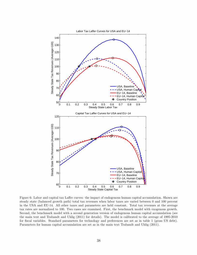
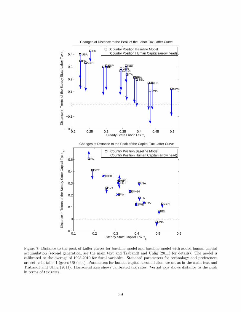
Figure 6 shows the comparison for the US and EU-14. Further cross-country results are contained

in figure 7. Interestingly, the capital tax Laffer curve is affected only very little across countries

when human capital is introduced. By contrast, the introduction of human capital has important

effects for the labor income tax Laffer curve. Several countries are pushed on the slippery slope

sides of their labor tax Laffer curves. This result is due to two effects. First, human capital

turns labor into a stock variable rather than a flow variable as in the baseline model. Higher

labor taxes induce households to work less and to aquire less human capital which in turn leads

to lower labor income. Consequently, the labor tax base shrinks much more quickly when labor

taxes are raised. Second, the introduction of intermediate inputs moves countries closer to the

peaks of their labor tax Laffer curves already in the baseline model compared to Trabandt and

Uhlig (2011). This effect is reinforced when human capital is introduced.

17

Finally, we recalculate the implied maximum interest rates on government debt in 2010 when

human capital accumulation is allowed for in the model. Table 9 contains the results: the US

may only afford a real interest rate between 5.8% to 6.6% in this case. Most of the European

countries cluster between 4% and 4.9% except for Denmark, Finland and Ireland who can afford

real interest rates between 5.9% and 9.5%.

5.2. Consumption taxes

We compute maximum additional tax revenues that are possible from increasing consumption

taxes. We do this in the above baseline model and in the model with added human capital

accumulation as in the previous subsection. The model is calibrated to the average of 1995-2010

for fiscal variables. Standard parameters for technology and preferences are set as in table 1.

Parameters for human capital accumulation are set as in the previous subsection.

The upper panel of figure 8 shows the comparison for the US and EU-14. Further cross-country

results are shown in the lower panel of the same figure. As documented and examined in Trabandt

and Uhlig (2011), the consumption tax Laffer curve has no peak. However, the introduction

of human capital has important quantitative effects across countries. The range of maximum

additional tax revenues (in percent of GDP) in the above baseline model is roughly 40-100

percent while it shrinks to roughly 10-30 percent in the model with added human capital. Higher

consumption taxes affect equilibrium labor via the labor wedge, similar to labor taxes. Human

capital amplifies the reduction of the labor tax base triggered by the change in the labor wedge

by the same argument as in the previous subsection. Overall, maximum possible tax revenues

due to consumption taxes are reduced massively, although at fairly high consumption tax rates.

6. Conclusion

We have studied how Laffer curves differ across countries in the US and the EU-14. This provides

insight into the limits of taxation. To that end, we extended the analysis in Trabandt and

Uhlig (2011) to include monopolistic competition as well as partial taxation of the monopolistic-

competition profits: we have shown that this improves the fit to the data considerably. We

have also provided refined data for effective labor and capital income taxes across countries.

18

For the cross-country comparison, we assume that all structural parameters for technologies and

preferences are the same across countries. The differences between the Laffer curves therefore

arise solely due to differences in fiscal policy i.e. the mix of distortionary taxes, government

spending and government debt. We find that labor income and consumption taxes are important

for accounting for most of the cross-country differences.

To examine recent developments, we calibrate the steady state of the model to the Laffer curves

implied by the strained fiscal situation of 2010, and compare them to the Laffer curves of the

average extended sample 1995-2010. We find that the 2010 calibration moves all countries con-

siderably closer to the peak of the labor tax Laffer curve, with the scope for additional labor

tax increases cut by a third for most countries and by up to one half for some countries. In this

context, we show that it is important to keep the general equilibrium repercussions of raising

taxes in mind: even though tax revenues may be increased by some limited amount, tax bases

and thereby output fall when moving to the peak of the Laffer curve due to the negative incentive

effects of higher taxes.

We calculate the implications for the long-term sustainability of current debt levels, by calculat-

ing the maximal permanently sustainable interest rate. We calculated that the USA can afford

the highest interest rate if only labor taxes are adjusted to service the additional debt burden:

depending on the debt measure used, a real interest rate of of 12% to 15.5% is sustainable.

Interestingly, Ireland can also afford the high rate of 11.2%, when moving labor taxes only. By

contrast, Austria, Belgium, Denmark, Finland, France, Greece and Italy can only afford perma-

nent real rates in the range of 4.4% to 7.1%, when financing the additional interest payments

with higher labor tax rates alone, while, say, Germany, Portugal and Spain can all afford an

interest rate somewhere above 9%. The picture improves somewhat, but not much, when labor

taxes and capital taxes can both be adjusted: notably, Belgium, Denmark, Finland, France and

Italy cannot permanently afford real interest rates above 6.5%.

We have shown that the introduction of human capital has important effects for the labor income

tax Laffer curve across countries. Several countries are pushed on the slippery slope sides of

their labor tax Laffer curves once human capital is accounted for. We recalculated the implied

maximum interest rates on government debt in 2010 when human capital accumulation is allowed

19

for in the model. In this case, the US may only afford a real interest rate between 5.8% to 6.6%.

Most of the European countries cluster between 4% and 4.9% except for Denmark, Finland and

Ireland who can afford real interest rates between 5.9% and 9.5%.

We have performed a cross-country analysis on consumption taxes. We document that the range

of maximum additional tax revenues (in percent of GDP) in the baseline model is roughly 40-

100 percent while it shrinks to roughly 10-30 percent in the model with added human capital,

although the underlying consumption taxes are fairly high in both cases.

References

Acemoglu, D., 2008. Introduction to Modern Economic Growth, 1st Edition. Princeton University

Press, Princeton.

Alesina, A., Glaeser, E., Sacerdote, B., 2006. Work and leisure in the US and Europe: Why so

different? NBER Macroeconomic Annual 2005, Vol. 20, MIT Press, Cambridge, pp. 1–100.

Barro, R. J., i Martin, X. S., 2003. Economic Growth, 2nd Edition. MIT Press, Cambridge.

Bi, H., 2010. Sovereign default risk premia, fiscal limits, and fiscal policy. Unpublished

Manuscript.

Bi, H., Leeper, E. M., Leith, C., 2010. Stabilization versus sustainability: Macroeconomic policy

tradeoffs. Unpublished Manuscript.

Blanchard, O., 2004. The economic future of europe. Journal Of Economic Perspectives 18(4),

3–26.

Chari, V. V., Kehoe, P. J., Mcgrattan, E. R., 2007. Business cycle accounting. Econometrica

75 (3), 781–836.

Cooley, T. F., Prescott, E., 1995. Economic growth and business cycles. In: T. F. Cooley (Ed.),

Frontiers Of Business Cycle Research, Princeton University Press, Princeton, pp. 1–38.

20

Green, J., Kotlikoff, L. J., 2009. On the general relativity of fiscal language. Key Issues in Public

Finance - A Conference in Memory of David Bradford, Eds. Alan J. Auerbach And Daniel

Shaviro, Harvard University Press.

Hall, R. E., 2009. Reconciling cyclical movements in the marginal value of time and the marginal

product of labor. Journal of Political Economy 117 (2), 281–323.

Jones, C. I., 2001. Introduction to Economic Growth, 2nd Edition. Norton, New York.

Kimball, M. S., Shapiro, M. D., 2008. Labor supply: Are the income and substitution effects

both large or both small? NBER Working Paper 14208, NBER.

King, R. S., Rebelo, S. T., 1999. Resuscitating real business cycles. In: J. B. Taylor And M.

Woodford (Eds.), Handbook Of Macroeconomics, Amsterdam: Elsevier 1B, pp. 927–1007.

Levine, R., Renelt, D., 1992. A sensitivity analysis of cross-country growth regressions. American

Economic Review 82(4), 942–63.

Ljungqvist, L., Sargent, T. J., 2007. Do taxes explain european employment? Indivisible labor,

human capital, lotteries, and savings. NBER Macroeconomics Annual 2006, Vol. 21, MIT

Press, Cambridge, pp. 181–246.

Lucas, R. E., 1988. On the mechanics of economic development. Journal of Monetary Economics

22, 3–42.

Mendoza, E. G., Razin, A., Tesar, L. L., 1994. Effective tax rates in macroeconomics: Cross-

country estimates of tax rates on factor incomes and consumption. Journal Of Monetary Eco-

nomics 34, 297–323.

Pissarides, C., Ngai, L. R., 2009. Welfare policy and the sectoral distribution of employment.

Center for Structual Econometrics Discussion Paper No. 09/04, London School of Economics.

Prescott, E. C., 2002. Prosperity and depression. American Economic Review 92, 1–15.

Prescott, E. C., 2004. Why do americans work so much more than europeans? Quarterly Review,

Federal Reserve Bank Of Minneapolis 28, 2–13.

21

Prescott, E. C., 2006. Nobel lecture: The transformation of macroeconomic policy and research.

Journal Of Political Economy 114(2), 203–235.

Rogerson, R., 2007. Taxation and market work: is Scandinavia an outlier? Economic Theory

32 (1), 59–85.

Shimer, R., 2009. Convergence in macroeconomics: The labor wedge. American Economic Jour-

nal: Macroeconomics 1(1), 280–297.

Trabandt, M., Uhlig, H., May 2011. The Laffer curve revisited. Journal of Monetary Economics

58 (4), 305–327.

Uzawa, H., 1965. Optimum technical change in an aggregative model of economic growth. Inter-

national Economic Review 6, 18–31.

7. Tables and Figures

22

Baseline calibration and parameterization

Variable US EU-14 Description Restriction

Fiscal Policyτn 22.1 34.2 Labor tax rate Dataτ k 41.1 36.8 Capital tax rate Dataτ c 4.6 16.7 Consumption tax rate Data

g/y 18.0 23.1 Gov. consumption+invest. to GDP DataGross Government Debt

b/y 66.2 67.3 Government gross debt to GDP Data

s/y 4.3 11.1 Government transfers to GDP ImpliedSensitivity: Government Debt Held By The Public

b/y 42.4 - Government debt held by public to GDP Data

s/y 4.9 - Government transfers to GDP ImpliedTrade

m/y 3.6 -1.2 Net imports to GDP DataTechnology

ψ 1.5 1.5 Annual balanced growth rate Dataθ 0.36 0.36 Capital share in production Dataδ 0.07 0.07 Annual depreciation rate of capital Data

R− 1 4 4 Annual real interest rate Dataω 1.1 1.1 Gross markup Dataϕ 0.36 0.36 Share of profits subject to capital taxes Data

CFE Preferencesη 2 2 Inverse of IES Dataφ 1 1 Frisch labor supply elasticity Dataκ 3.30 3.30 Weight of labor nus = 0.25

Table 1: Baseline calibration and parameterization for the US and EU-14 benchmark model. Numbers expressedin percent where applicable. Sample: 1995-2010. IES denotes intertemporal elasticity of substitution. CFE refersto constant Frisch elasticity preferences. nus denotes balanced growth labor in the US which is set to 25 percentof total time.

23

Calibration of the model to individual countries

τn τ c τ k b/y m/y g/y s/y∅ 2010a 2010b ∅ 2010 ∅ 2010 ∅ 2010 ∅ 2010 ∅ 2010 ∅ 2010

USA 22 20 28 5 4 41 38 66 92 4 4 18 20 4 4USA∗ 22 20 28 5 4 41 38 42 64 4 4 18 20 5 5EU-14 34 35 40 17 15 37 36 67 83 -1 -1 23 25 11 11GER 34 35 35 16 17 25 27 64 83 -3 -5 21 21 10 10FRA 39 39 43 18 16 43 43 63 82 -0 2 27 28 12 12ITA 36 39 39 14 13 41 45 111 119 -1 2 22 23 13 13GBR 24 25 36 15 13 52 50 48 80 2 3 22 26 11 11AUT 43 43 45 20 20 26 24 66 72 -3 -5 21 21 18 18BEL 39 38 43 17 17 51 50 104 97 -4 -3 24 26 16 16DNK 43 44 50 34 31 49 56 49 44 -5 -6 28 32 22 22FIN 44 41 51 26 23 31 30 45 48 -6 -3 25 27 17 17GRE 29 28 35 15 13 19 17 105 143 10 8 21 21 6 6IRL 25 24 40 24 19 17 16 48 96 -13 -19 19 23 7 7NET 36 38 50 19 19 32 23 58 63 -7 -8 27 32 6 6PRT 22 24 30 19 16 32 34 61 93 9 7 23 24 7 7ESP 30 30 42 14 10 31 24 54 60 3 2 22 24 8 8SWE 50 46 43 26 26 40 52 54 40 -7 -6 30 31 16 16

Table 2: Individual country calibration of the benchmark model for the average (∅) sample 1995-2010 and forthe year 2010. Country codes: Germany (GER), France (FRA), Italy (ITA), United Kingdom (GBR), Austria(AUT), Belgium (BEL), Denmark (DNK), Finland (FIN), Greece (GRE), Ireland (IRL), Netherlands (NET),Portugal (PRT), Spain (ESP) and Sweden (SWE). See table 1 for abbreviations of variables. All numbers areexpressed in percent. a - due to data availability reasons, the year 2009 value for tax rates has been assumed toremain in 2010 for most of the analysis in this paper. b - we deviate from a in subsection 3.2 by letting labor taxesin 2010 adjust to balance the 2010 government budget. More precisely, we calculate the 2010 labor tax givengovernment debt and consumption in 2010 as well as average (1995-2010) model implied transfers. ∗ - resultswhen “debt held by the public” is used for the USA rather than the harmonized cross-country measure of grossgovernment debt provided by the AMECO database.

24

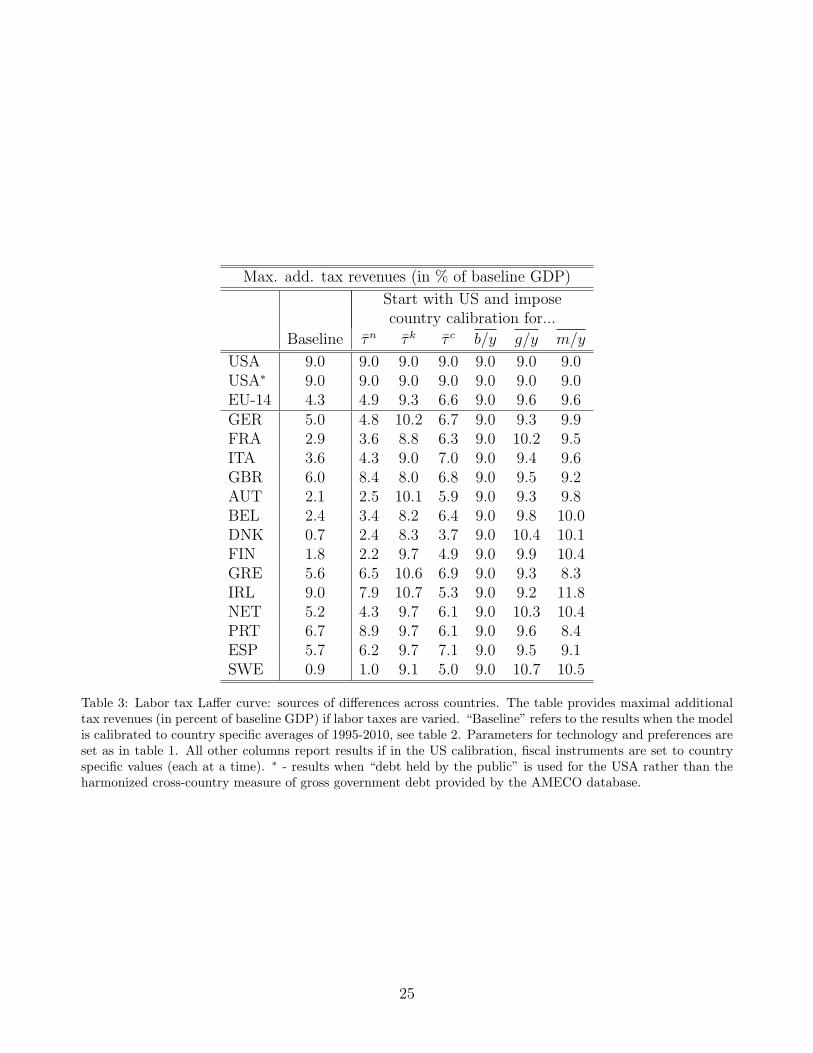
Max. add. tax revenues (in % of baseline GDP)

Start with US and imposecountry calibration for...

Baseline τn τ k τ c b/y g/y m/y

USA 9.0 9.0 9.0 9.0 9.0 9.0 9.0USA∗ 9.0 9.0 9.0 9.0 9.0 9.0 9.0EU-14 4.3 4.9 9.3 6.6 9.0 9.6 9.6GER 5.0 4.8 10.2 6.7 9.0 9.3 9.9FRA 2.9 3.6 8.8 6.3 9.0 10.2 9.5ITA 3.6 4.3 9.0 7.0 9.0 9.4 9.6GBR 6.0 8.4 8.0 6.8 9.0 9.5 9.2AUT 2.1 2.5 10.1 5.9 9.0 9.3 9.8BEL 2.4 3.4 8.2 6.4 9.0 9.8 10.0DNK 0.7 2.4 8.3 3.7 9.0 10.4 10.1FIN 1.8 2.2 9.7 4.9 9.0 9.9 10.4GRE 5.6 6.5 10.6 6.9 9.0 9.3 8.3IRL 9.0 7.9 10.7 5.3 9.0 9.2 11.8NET 5.2 4.3 9.7 6.1 9.0 10.3 10.4PRT 6.7 8.9 9.7 6.1 9.0 9.6 8.4ESP 5.7 6.2 9.7 7.1 9.0 9.5 9.1SWE 0.9 1.0 9.1 5.0 9.0 10.7 10.5

Table 3: Labor tax Laffer curve: sources of differences across countries. The table provides maximal additionaltax revenues (in percent of baseline GDP) if labor taxes are varied. “Baseline” refers to the results when the modelis calibrated to country specific averages of 1995-2010, see table 2. Parameters for technology and preferences areset as in table 1. All other columns report results if in the US calibration, fiscal instruments are set to countryspecific values (each at a time). ∗ - results when “debt held by the public” is used for the USA rather than theharmonized cross-country measure of gross government debt provided by the AMECO database.

25

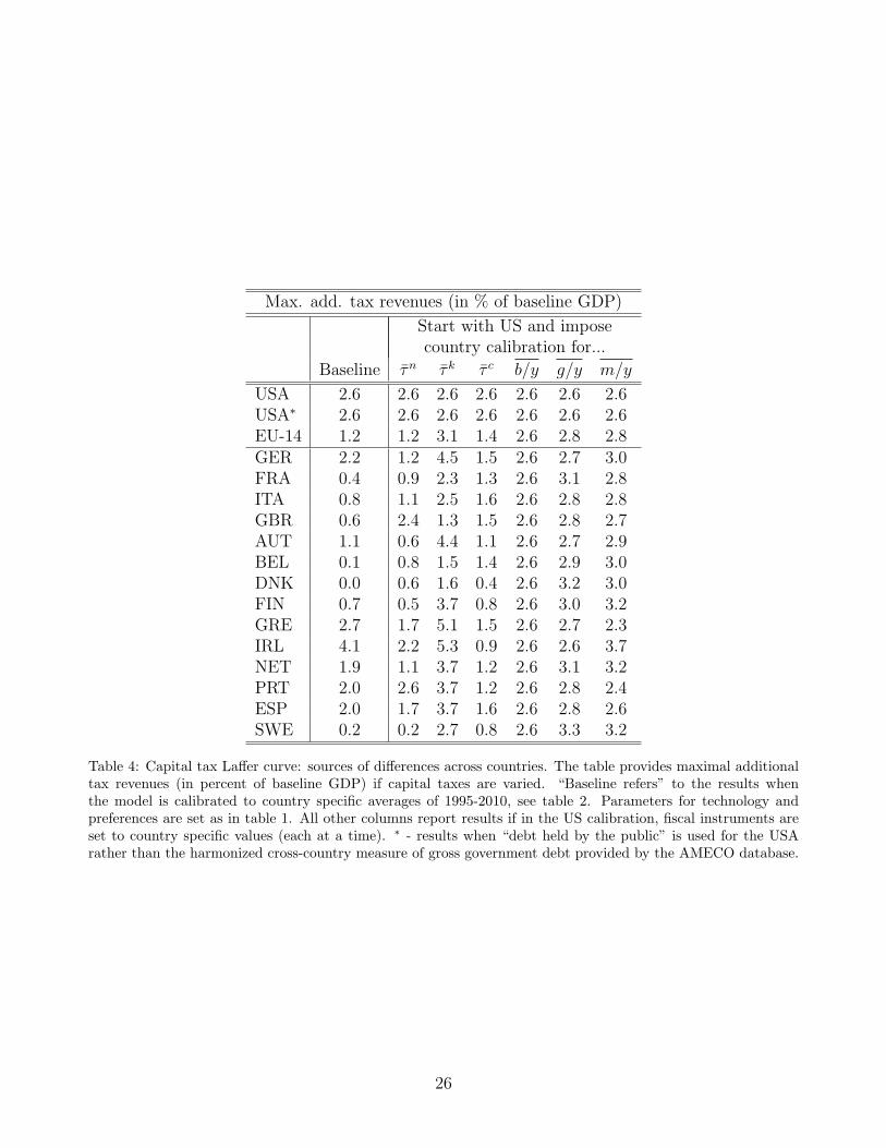
Max. add. tax revenues (in % of baseline GDP)

Start with US and imposecountry calibration for...

Baseline τn τ k τ c b/y g/y m/y

USA 2.6 2.6 2.6 2.6 2.6 2.6 2.6USA∗ 2.6 2.6 2.6 2.6 2.6 2.6 2.6EU-14 1.2 1.2 3.1 1.4 2.6 2.8 2.8GER 2.2 1.2 4.5 1.5 2.6 2.7 3.0FRA 0.4 0.9 2.3 1.3 2.6 3.1 2.8ITA 0.8 1.1 2.5 1.6 2.6 2.8 2.8GBR 0.6 2.4 1.3 1.5 2.6 2.8 2.7AUT 1.1 0.6 4.4 1.1 2.6 2.7 2.9BEL 0.1 0.8 1.5 1.4 2.6 2.9 3.0DNK 0.0 0.6 1.6 0.4 2.6 3.2 3.0FIN 0.7 0.5 3.7 0.8 2.6 3.0 3.2GRE 2.7 1.7 5.1 1.5 2.6 2.7 2.3IRL 4.1 2.2 5.3 0.9 2.6 2.6 3.7NET 1.9 1.1 3.7 1.2 2.6 3.1 3.2PRT 2.0 2.6 3.7 1.2 2.6 2.8 2.4ESP 2.0 1.7 3.7 1.6 2.6 2.8 2.6SWE 0.2 0.2 2.7 0.8 2.6 3.3 3.2

Table 4: Capital tax Laffer curve: sources of differences across countries. The table provides maximal additionaltax revenues (in percent of baseline GDP) if capital taxes are varied. “Baseline refers” to the results whenthe model is calibrated to country specific averages of 1995-2010, see table 2. Parameters for technology andpreferences are set as in table 1. All other columns report results if in the US calibration, fiscal instruments areset to country specific values (each at a time). ∗ - results when “debt held by the public” is used for the USArather than the harmonized cross-country measure of gross government debt provided by the AMECO database.

26

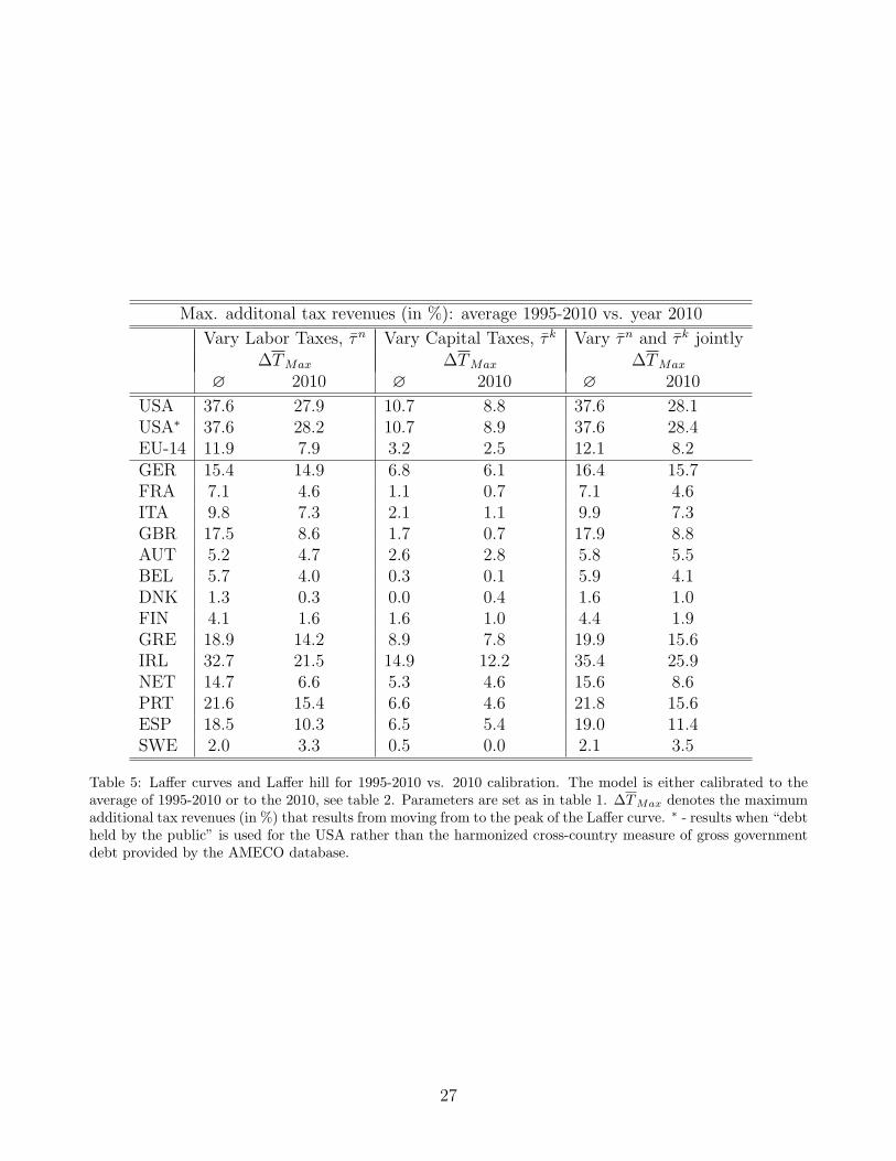
Max. additonal tax revenues (in %): average 1995-2010 vs. year 2010

Vary Labor Taxes, τn Vary Capital Taxes, τ k Vary τn and τ k jointly∆TMax ∆TMax ∆TMax

∅ 2010 ∅ 2010 ∅ 2010

USA 37.6 27.9 10.7 8.8 37.6 28.1USA∗ 37.6 28.2 10.7 8.9 37.6 28.4EU-14 11.9 7.9 3.2 2.5 12.1 8.2GER 15.4 14.9 6.8 6.1 16.4 15.7FRA 7.1 4.6 1.1 0.7 7.1 4.6ITA 9.8 7.3 2.1 1.1 9.9 7.3GBR 17.5 8.6 1.7 0.7 17.9 8.8AUT 5.2 4.7 2.6 2.8 5.8 5.5BEL 5.7 4.0 0.3 0.1 5.9 4.1DNK 1.3 0.3 0.0 0.4 1.6 1.0FIN 4.1 1.6 1.6 1.0 4.4 1.9GRE 18.9 14.2 8.9 7.8 19.9 15.6IRL 32.7 21.5 14.9 12.2 35.4 25.9NET 14.7 6.6 5.3 4.6 15.6 8.6PRT 21.6 15.4 6.6 4.6 21.8 15.6ESP 18.5 10.3 6.5 5.4 19.0 11.4SWE 2.0 3.3 0.5 0.0 2.1 3.5

Table 5: Laffer curves and Laffer hill for 1995-2010 vs. 2010 calibration. The model is either calibrated to theaverage of 1995-2010 or to the 2010, see table 2. Parameters are set as in table 1. ∆TMax denotes the maximumadditional tax revenues (in %) that results from moving from to the peak of the Laffer curve. ∗ - results when “debtheld by the public” is used for the USA rather than the harmonized cross-country measure of gross governmentdebt provided by the AMECO database.

27

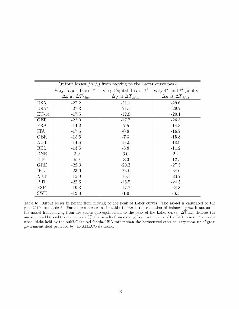
Output losses (in %) from moving to the Laffer curve peak

Vary Labor Taxes, τn Vary Capital Taxes, τ k Vary τn and τ k jointly∆y at ∆TMax ∆y at ∆TMax ∆y at ∆TMax

USA -27.2 -21.1 -29.6USA∗ -27.3 -21.1 -29.7EU-14 -17.5 -12.8 -20.1GER -22.0 -17.7 -26.5FRA -14.2 -7.5 -14.3ITA -17.6 -8.8 -16.7GBR -18.5 -7.3 -15.8AUT -14.6 -13.0 -18.9BEL -13.6 -3.8 -11.2DNK -3.9 6.0 2.2FIN -9.0 -8.3 -12.5GRE -22.3 -20.3 -27.5IRL -23.6 -23.6 -34.6NET -15.9 -16.1 -23.7PRT -22.6 -16.5 -24.5ESP -19.3 -17.7 -24.8SWE -12.3 -1.0 -8.5

Table 6: Output losses in perent from moving to the peak of Laffer curves. The model is calibrated to theyear 2010, see table 2. Parameters are set as in table 1. ∆y is the reduction of balanced growth output inthe model from moving from the status quo equilibrium to the peak of the Laffer curve. ∆TMax denotes themaximum additional tax revenues (in %) that results from moving from to the peak of the Laffer curve. ∗ - resultswhen “debt held by the public” is used for the USA rather than the harmonized cross-country measure of grossgovernment debt provided by the AMECO database.

28

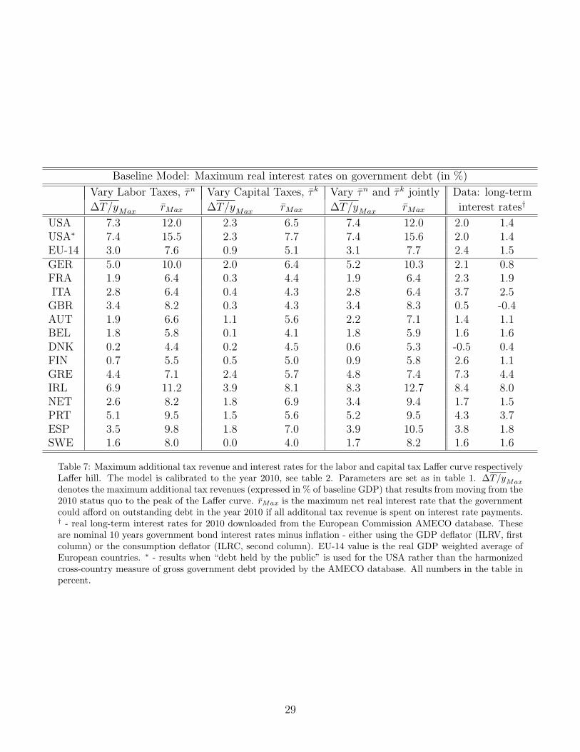
Baseline Model: Maximum real interest rates on government debt (in %)

Vary Labor Taxes, τn Vary Capital Taxes, τ k Vary τn and τ k jointly Data: long-term

∆T/yMax rMax ∆T/yMax rMax ∆T/yMax rMax interest rates†

USA 7.3 12.0 2.3 6.5 7.4 12.0 2.0 1.4USA∗ 7.4 15.5 2.3 7.7 7.4 15.6 2.0 1.4EU-14 3.0 7.6 0.9 5.1 3.1 7.7 2.4 1.5GER 5.0 10.0 2.0 6.4 5.2 10.3 2.1 0.8FRA 1.9 6.4 0.3 4.4 1.9 6.4 2.3 1.9ITA 2.8 6.4 0.4 4.3 2.8 6.4 3.7 2.5GBR 3.4 8.2 0.3 4.3 3.4 8.3 0.5 -0.4AUT 1.9 6.6 1.1 5.6 2.2 7.1 1.4 1.1BEL 1.8 5.8 0.1 4.1 1.8 5.9 1.6 1.6DNK 0.2 4.4 0.2 4.5 0.6 5.3 -0.5 0.4FIN 0.7 5.5 0.5 5.0 0.9 5.8 2.6 1.1GRE 4.4 7.1 2.4 5.7 4.8 7.4 7.3 4.4IRL 6.9 11.2 3.9 8.1 8.3 12.7 8.4 8.0NET 2.6 8.2 1.8 6.9 3.4 9.4 1.7 1.5PRT 5.1 9.5 1.5 5.6 5.2 9.5 4.3 3.7ESP 3.5 9.8 1.8 7.0 3.9 10.5 3.8 1.8SWE 1.6 8.0 0.0 4.0 1.7 8.2 1.6 1.6

Table 7: Maximum additional tax revenue and interest rates for the labor and capital tax Laffer curve respectivelyLaffer hill. The model is calibrated to the year 2010, see table 2. Parameters are set as in table 1. ∆T/yMax

denotes the maximum additional tax revenues (expressed in % of baseline GDP) that results from moving from the2010 status quo to the peak of the Laffer curve. rMax is the maximum net real interest rate that the governmentcould afford on outstanding debt in the year 2010 if all additonal tax revenue is spent on interest rate payments.† - real long-term interest rates for 2010 downloaded from the European Commission AMECO database. Theseare nominal 10 years government bond interest rates minus inflation - either using the GDP deflator (ILRV, firstcolumn) or the consumption deflator (ILRC, second column). EU-14 value is the real GDP weighted average ofEuropean countries. ∗ - results when “debt held by the public” is used for the USA rather than the harmonizedcross-country measure of gross government debt provided by the AMECO database. All numbers in the table inpercent.

29

Distance to Peak in Terms of Tax Rates (in %)Vary Labor Taxes, τn Vary Capital Taxes, τ k

Baseline Human Capital Baseline Human Capital

USA 39.9 20.9 29.9 27.9USA∗ 39.9 20.9 29.9 27.9EU-14 26.8 7.8 23.2 22.2GER 28.5 11.5 36.1 36.1FRA 21.4 1.4 13.6 12.6ITA 23.8 3.8 17.7 15.7GBR 33.2 11.2 12.9 9.9AUT 17.2 -3.8 26.3 22.3BEL 19.7 -1.3 6.5 4.5DNK 10.7 -15.3 -2.4 -5.4FIN 17.0 -4.0 20.5 20.5GRE 29.9 7.9 41.0 34.0IRL 42.8 34.8 50.7 56.7NET 30.9 17.9 32.3 36.3PRT 34.8 12.8 30.3 26.3ESP 31.0 12.0 31.9 28.9SWE 12.2 -8.8 12.2 13.2

Table 8: Distance to the peak of Laffer curves for baseline model and baseline model with added human capitalaccumulation (second generation, see the main text and Trabandt and Uhlig (2011) for details). Distance ismeasured in terms of tax rates. All numbers are expressed in percent. The model is calibrated to the average of1995-2010 for fiscal variables. Standard parameters for technology and preferences are set as in table 1. Parametersfor human capital accumulation are set as in the main text and Trabandt and Uhlig (2011). ∗ - results when “debtheld by the public” is used for the USA rather than the harmonized cross-country measure of gross governmentdebt provided by the AMECO database. All numbers in the table in percent.

30

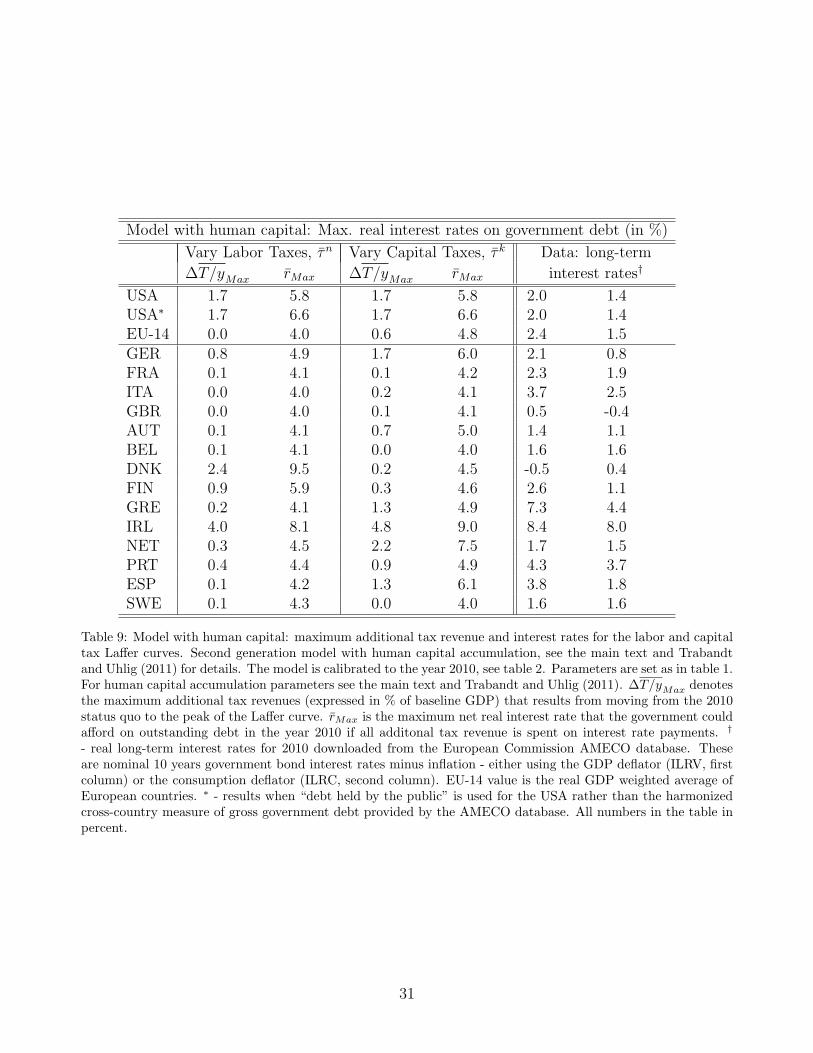
Model with human capital: Max. real interest rates on government debt (in %)

Vary Labor Taxes, τn Vary Capital Taxes, τ k Data: long-term

∆T/yMax rMax ∆T/yMax rMax interest rates†

USA 1.7 5.8 1.7 5.8 2.0 1.4USA∗ 1.7 6.6 1.7 6.6 2.0 1.4EU-14 0.0 4.0 0.6 4.8 2.4 1.5GER 0.8 4.9 1.7 6.0 2.1 0.8FRA 0.1 4.1 0.1 4.2 2.3 1.9ITA 0.0 4.0 0.2 4.1 3.7 2.5GBR 0.0 4.0 0.1 4.1 0.5 -0.4AUT 0.1 4.1 0.7 5.0 1.4 1.1BEL 0.1 4.1 0.0 4.0 1.6 1.6DNK 2.4 9.5 0.2 4.5 -0.5 0.4FIN 0.9 5.9 0.3 4.6 2.6 1.1GRE 0.2 4.1 1.3 4.9 7.3 4.4IRL 4.0 8.1 4.8 9.0 8.4 8.0NET 0.3 4.5 2.2 7.5 1.7 1.5PRT 0.4 4.4 0.9 4.9 4.3 3.7ESP 0.1 4.2 1.3 6.1 3.8 1.8SWE 0.1 4.3 0.0 4.0 1.6 1.6

Table 9: Model with human capital: maximum additional tax revenue and interest rates for the labor and capitaltax Laffer curves. Second generation model with human capital accumulation, see the main text and Trabandtand Uhlig (2011) for details. The model is calibrated to the year 2010, see table 2. Parameters are set as in table 1.For human capital accumulation parameters see the main text and Trabandt and Uhlig (2011). ∆T/yMax denotesthe maximum additional tax revenues (expressed in % of baseline GDP) that results from moving from the 2010status quo to the peak of the Laffer curve. rMax is the maximum net real interest rate that the government couldafford on outstanding debt in the year 2010 if all additonal tax revenue is spent on interest rate payments. †

- real long-term interest rates for 2010 downloaded from the European Commission AMECO database. Theseare nominal 10 years government bond interest rates minus inflation - either using the GDP deflator (ILRV, firstcolumn) or the consumption deflator (ILRC, second column). EU-14 value is the real GDP weighted average ofEuropean countries. ∗ - results when “debt held by the public” is used for the USA rather than the harmonizedcross-country measure of gross government debt provided by the AMECO database. All numbers in the table inpercent.

31

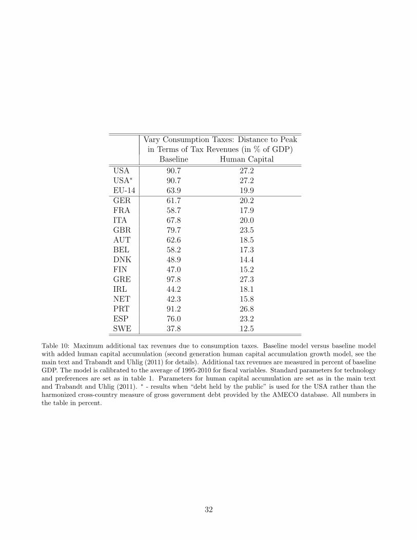
Vary Consumption Taxes: Distance to Peakin Terms of Tax Revenues (in % of GDP)

Baseline Human Capital

USA 90.7 27.2USA∗ 90.7 27.2EU-14 63.9 19.9GER 61.7 20.2FRA 58.7 17.9ITA 67.8 20.0GBR 79.7 23.5AUT 62.6 18.5BEL 58.2 17.3DNK 48.9 14.4FIN 47.0 15.2GRE 97.8 27.3IRL 44.2 18.1NET 42.3 15.8PRT 91.2 26.8ESP 76.0 23.2SWE 37.8 12.5

Table 10: Maximum additional tax revenues due to consumption taxes. Baseline model versus baseline modelwith added human capital accumulation (second generation human capital accumulation growth model, see themain text and Trabandt and Uhlig (2011) for details). Additional tax revenues are measured in percent of baselineGDP. The model is calibrated to the average of 1995-2010 for fiscal variables. Standard parameters for technologyand preferences are set as in table 1. Parameters for human capital accumulation are set as in the main textand Trabandt and Uhlig (2011). ∗ - results when “debt held by the public” is used for the USA rather than theharmonized cross-country measure of gross government debt provided by the AMECO database. All numbers inthe table in percent.

32

2.5

33.

5

2.53

3.5

GE

R

FR

A

ITA

GB

R

AU

T

BE

L

DN

K

FIN

GR

E

IRL

NE

T

PR

T

ES

P

SW

E

US

A

EU

−14

Cap

ital t

o G

DP

0.2

0.22

0.24

0.26

0.2

0.22

0.24

0.26

GE

R

FR

A

ITA

GB

R

AU

T

BE

L

DN

K

FIN

G

RE

IRL

NE

T

PR

T

ES

P

SW

E

US

A EU

−14

Actual (Data)

Inve

stm

ent t

o G

DP

0.2

0.22

0.24

0.26

0.28

0.2

0.22

0.24

0.26

0.28

GE

R

FR

A

ITA

G

BR

AU

T B

EL

DN

K F

IN

GR

E

IRL

NE

T

PR

T

ES

P

SW

E

US

A

EU

−14

Hou

rs

0.45

0.5

0.55

0.6

0.65

0.450.5

0.550.6

0.65

GE

R

FR

A

ITA

GB

R

AU

T

BE

L

DN

K

FIN

GR

E

IRL

NE

T

PR

T

ES

P

SW

E

US

A

EU

−14

Con

sum

ptio

n to

GD

P

0.15

0.2

0.25

0.150.2

0.25

GE

R

FR

A

ITA

GB

R

AU

T

BE

L D

NK

F

IN

GR

E

IRL

NE

T

PR

T

ES

P

SW

E

US

A

EU

−14

Actual (Data)

Pre

dict

ed

Labo

r ta

x re

venu

es to

GD

P

0.04

0.06

0.08

0.1

0.04

0.06

0.080.1

GE

R

FR

A

ITA

G

BR

AU

T

BE

L

DN

K

FIN

GR

E

IRL

N

ET

PR

T

ES

P

SW

E

US

A

EU

−14

Pre

dict

ed

Cap

ital t

ax r

even

ues

to G

DP

0.05

0.1

0.15

0.050.1

0.15

GE

R FR

A

ITA

GB

R AU

T

BE

L

DN

K

FIN

GR

E

IRL

N

ET

P

RT

ES

P

SW

E

US

A

EU

−14

Pre

dict

ed

Con

sum

ptio

n ta

x re

venu

es to

GD

P

0.05

0.1

0.15

0.2

0.050.1

0.150.2

GE

R F

RA

IT

A

GB

R

AU

T

BE

L

DN

K

FIN

GR

E

IRL

N

ET

PR

T ES

P

SW

E

US

A

EU

−14

Net

tran

sfer

s to

GD

P

0.3

0.4

0.5

0.250.3

0.350.4

0.450.5

GE

R

FR

A

ITA

GB

R

AU

T B

EL

DN

K

FIN

GR

E

IRL

NE

T

PR

T

ES

P

SW

E

US

A

EU

−14

Actual (Data)

Tot

al ta

x re

venu

es to

GD

P

Figure

1:Com

parison

of“a

ctual”

vs.

“predicted”variab

les.

“Actual”refers

todatasample

averag

esfor19

95-201

0.“P

redicted”refers

tomodel

implied

steadystate

(balancedgrow

thpath)variab

leswhen

themodel

iscalibratedas

intable

2(gross

USdeb

t).Param

etersfortechnologyand

preferencesare

setas

intable

1(gross

debt).

33

0.25

0.3

0.35

0.4

0.45

0.5

0.250.3

0.350.4

0.450.5

Actual (Data)

Tot

al ta

x re

venu

es to

GD

P

Ben

chm

ark

(ω=

1.1

,φ=

0.3

6)

ω→

1φ

=1

0.05

0.1

0.15

0.2

0.050.1

0.150.2

Net

tran

sfer

s to

GD

P

0.15

0.2

0.25

0.3

0.12

0.14

0.16

0.180.2

0.22

0.24

0.26

0.280.3

Actual (Data)

Pre

dict

ed

Labo

r ta

x re

venu

es to

GD

P

0.04

0.06

0.08

0.1

0.12

0.04

0.06

0.080.1

0.12

Pre

dict

ed

Cap

ital t

ax r

even

ues

to G

DP

Figure

2:Sensitivityof“a

ctual”vs.

“predicted”taxrevenues

andgovernmenttran

sfers.

“Actual”refers

todatasample

averag

esfor1995-2010.

“Predicted”refers

tomodel

implied

steadystate(balan

cedgrow

thpath).

Threecasesareexam

ined

.Theben

chmarkcase

isthemodel

usedin

the

pap

er,an

das

infigu

re1.

Thecase

ω→

1obtains,when

thereisnomarket

pow

erbyinterm

ediate

goodsproducers:thisisou

rpreviouslyusedmodel

inTrabandtan

dUhlig(201

1).Finally,thereis

theinterm

ediate

case

withmon

opolisticcompetition,butwhereprofits

arefullysubject

tocapital

taxation,ϕ=

1.Note

thatallother

variablesplotted

infigu

re1areunaff

ectedbythesensitivityan

alysis,

exceptforhou

rs.How

ever,theim

pact

on

hou

rsis

smallan

dthereforeom

ittedhere.

Allother

param

etersan

dsteadystates

areas

intables1an

d2(gross

USdeb

t).

34

0.2 0.3 0.4 0.5 0.6 0.7 0.890

95

100

105

110

115

120

125

130

135

140

Steady State Labor Tax

Ste

ady

Sta

te T

ax R

even

ues

(Ave

rage

=10

0)

Labor Tax Laffer Curves Across Countries

GER

FRA ITA

GBR

AUT BEL

DNK FIN

GRE

IRL

NET

PRT

ESP

SWE

USA

EU−14

Country Pos. Avg. 95−2010

0.2 0.3 0.4 0.5 0.6 0.7 0.8

95

100

105

110

115

Steady State Capital Tax

Ste

ady

Sta

te T

ax R

even

ues

(Ave

rage

=10

0)

Capital Tax Laffer Curves Across Countries

GER

FRA ITA GBR

AUT

BEL DNK

FIN

GRE

IRL

NET PRT ESP

SWE

USA

EU−14

Country Position Avg. 95−2010

Figure 3: Labor and capital tax Laffer curves across all countries. The model is calibrated to the average of1995-2010, see table 2 (gross US debt). Parameters for technology and preferences are set as in table 1 (grossUS debt). Shown are steady state (balanced growth path) total tax revenues when labor taxes (upper panel)or capital taxes (lower panel) are varied between 0 and 100 percent. All other taxes and parameters are heldconstant. Total tax revenues at the average 1995-2010 tax rates are normalized to 100. Stars indicate positionsof respective countries on their Laffer curves. Note that the first letter of each country name indicates the peakof the respective Laffer curve.

35

0 0.1 0.2 0.3 0.4 0.5 0.6 0.7 0.8 0.950

60

70

80

90

100

110

120

130

140

Steady State Labor Tax

Ste

ady

Sta

te T

ax R

even

ues

(Ave

rage

=10

0)

Labor Tax Laffer Curves for USA and EU−14

USA, 1995−2010USA, 2010EU−14, 1995−2010EU−14, 2010Country Position

0 0.1 0.2 0.3 0.4 0.5 0.6 0.7 0.8 0.960

65

70

75

80

85

90

95

100

105

110

115

Steady State Capital Tax

Ste

ady

Sta

te T

ax R

even

ues

(Ave

rage

=10

0)

Capital Tax Laffer Curves for USA and EU−14

USA, 1995−2010USA, 2010EU−14, 1995−2010EU−14, 2010Country Position

Figure 4: Comparing the US and the EU-14 labor and capital tax Laffer curve. The model is either calibrated tothe average of 1995-2010 or to the 2010, see table 2 (gross US debt). Parameters for technology and preferencesare set as in table 1 (gross US debt). Shown are steady state (balanced growth path) total tax revenues whenlabor taxes (upper panel) or capital taxes (lower panel) are varied between 0 and 100 percent. All other taxesand parameters are held constant. Total tax revenues at the average 1995-2010 or at the year 2010 tax rates arenormalized to 100. Stars indicate positions of respective countries on their Laffer curves.

36

0.2 0.25 0.3 0.35 0.4 0.45 0.50

0.05

0.1

0.15

0.2

0.25

0.3

0.35

0.4

0.45

GER

FRA

ITA

GBR

AUT

BEL

DNK

FIN

GRE

IRL

NET

PRT

ESP

SWE

USA

EU−14

Changes of Distance to the Peak of the Labor Tax Laffer Curve

Steady State Labor Tax τn

Dis

tanc

e in

Ter

ms

of th

e S

tead

y S

tate

Lab

or T

ax τ

n

Country Position avg. 1995−2010Country Position 2010 (arrow head)Varying US Steady State Labor Tax

0.15 0.2 0.25 0.3 0.35 0.4 0.45 0.5 0.55

−0.1

0

0.1

0.2

0.3

0.4

0.5

0.6

GER

FRA

ITA

GBR

AUT

BEL

DNK

FIN

GRE

IRL

NET PRT

ESP

SWE

USA

EU−14

Changes of Distance to the Peak of the Capital Tax Laffer Curve

Steady State Capital Tax τk

Dis

tanc

e in

Ter

ms

of th

e S

tead

y S

tate

Cap

ital T

ax τ

k

Country Position avg. 1995−2010Country Position 2010 (arrow head)Varying US Steady State Capital Tax

Figure 5: Distance to the peak of Laffer curves for average 1995-2010 vs. 2010 calibration. The model is eithercalibrated to the average of 1995-2010 or to the 2010, see table 2 (gross US debt). Parameters for technology andpreferences are set as in table 1 (gross US debt). Horizontal axis shows calibrated tax rates. Vertial axis showsdistance to the peak in terms of tax rates. The dashed-dotted line shows the distance to the peak for the USwhen the initial steady state tax is varied and the model is re-calibrated for each assumed tax rate.

37

0 0.1 0.2 0.3 0.4 0.5 0.6 0.7 0.8 0.950

60

70

80

90

100

110

120

130

140

Steady State Labor Tax

Ste

ady

Sta

te T

ax R

even

ues

(Ave

rage

=10

0)

Labor Tax Laffer Curves for USA and EU−14

USA, BaselineUSA, Human CapitalEU−14, BaselineEU−14, Human CapitalCountry Position

0 0.1 0.2 0.3 0.4 0.5 0.6 0.7 0.8 0.960

70

80

90

100

110

120

Steady State Capital Tax

Ste

ady

Sta

te T

ax R

even

ues

(Ave

rage

=10

0)

Capital Tax Laffer Curves for USA and EU−14

USA, BaselineUSA, Human CapitalEU−14, BaselineEU−14, Human CapitalCountry Position

Figure 6: Labor and capital tax Laffer curves: the impact of endogenous human capital accumulation. Shown aresteady state (balanced growth path) total tax revenues when labor taxes are varied between 0 and 100 percentin the USA and EU-14. All other taxes and parameters are held constant. Total tax revenues at the averagetax rates are normalized to 100. Two cases are examined. First, the benchmark model with exogenous growth.Second, the benchmark model with a second generation version of endogenous human capital accumulation (seethe main text and Trabandt and Uhlig (2011) for details). The model is calibrated to the average of 1995-2010for fiscal variables. Standard parameters for technology and preferences are set as in table 1 (gross US debt).Parameters for human capital accumulation are set as in the main text Trabandt and Uhlig (2011).

38

0.2 0.25 0.3 0.35 0.4 0.45 0.5−0.2

−0.1

0

0.1

0.2

0.3

0.4

GER

FRA ITA

GBR

AUT BEL

DNK

FIN

GRE

IRL

NET

PRT

ESP

SWE

USA

EU−14

Changes of Distance to the Peak of the Labor Tax Laffer Curve

Steady State Labor Tax τn

Dis

tanc

e in

Ter

ms

of th

e S

tead

y S

tate

Lab

or T

ax τ

n

Country Position Baseline ModelCountry Position Human Capital (arrow head)

0.1 0.2 0.3 0.4 0.5 0.6−0.1

0

0.1

0.2

0.3

0.4

0.5

GER

FRA

ITA

GBR

AUT

BEL

DNK

FIN

GRE

IRL

NET PRT

ESP

SWE

USA

EU−14

Changes of Distance to the Peak of the Capital Tax Laffer Curve

Steady State Capital Tax τk

Dis

tanc

e in

Ter

ms

of th

e S

tead

y S

tate

Cap

ital T

ax τ

k

Country Position Baseline ModelCountry Position Human Capital (arrow head)

Figure 7: Distance to the peak of Laffer curves for baseline model and baseline model with added human capitalaccumulation (second generation, see the main text and Trabandt and Uhlig (2011) for details). The model iscalibrated to the average of 1995-2010 for fiscal variables. Standard parameters for technology and preferencesare set as in table 1 (gross US debt). Parameters for human capital accumulation are set as in the main text andTrabandt and Uhlig (2011). Horizontal axis shows calibrated tax rates. Vertial axis shows distance to the peakin terms of tax rates.

39

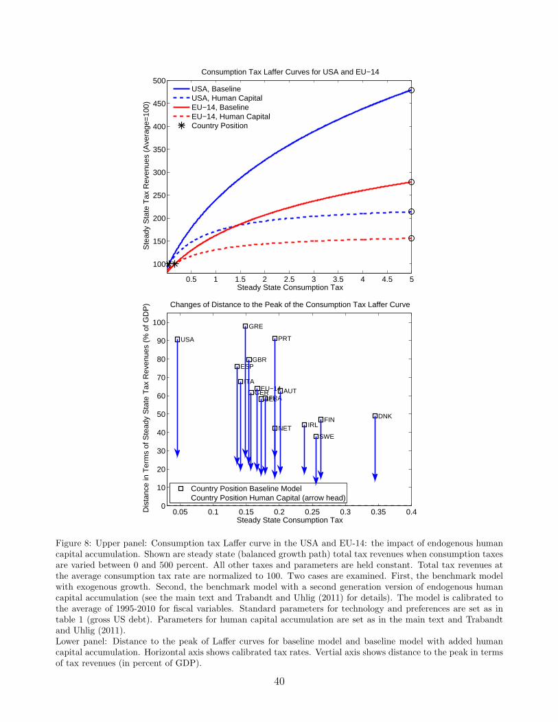
0.5 1 1.5 2 2.5 3 3.5 4 4.5 5

100

150

200

250

300

350

400

450

500

Steady State Consumption Tax

Ste

ady

Sta

te T

ax R

even

ues

(Ave

rage

=10

0)

Consumption Tax Laffer Curves for USA and EU−14

USA, BaselineUSA, Human CapitalEU−14, BaselineEU−14, Human CapitalCountry Position

0.05 0.1 0.15 0.2 0.25 0.3 0.35 0.40

10

20

30

40

50

60

70

80

90

100

GER FRA

ITA

GBR

AUT BEL

DNK FIN

GRE

IRL NET

PRT

ESP

SWE

USA

EU−14

Changes of Distance to the Peak of the Consumption Tax Laffer Curve

Steady State Consumption Tax

Dis

tanc

e in

Ter

ms

of S

tead

y S

tate

Tax

Rev

enue

s (%

of G

DP

)

Country Position Baseline ModelCountry Position Human Capital (arrow head)

Figure 8: Upper panel: Consumption tax Laffer curve in the USA and EU-14: the impact of endogenous humancapital accumulation. Shown are steady state (balanced growth path) total tax revenues when consumption taxesare varied between 0 and 500 percent. All other taxes and parameters are held constant. Total tax revenues atthe average consumption tax rate are normalized to 100. Two cases are examined. First, the benchmark modelwith exogenous growth. Second, the benchmark model with a second generation version of endogenous humancapital accumulation (see the main text and Trabandt and Uhlig (2011) for details). The model is calibrated tothe average of 1995-2010 for fiscal variables. Standard parameters for technology and preferences are set as intable 1 (gross US debt). Parameters for human capital accumulation are set as in the main text and Trabandtand Uhlig (2011).Lower panel: Distance to the peak of Laffer curves for baseline model and baseline model with added humancapital accumulation. Horizontal axis shows calibrated tax rates. Vertial axis shows distance to the peak in termsof tax revenues (in percent of GDP).

40

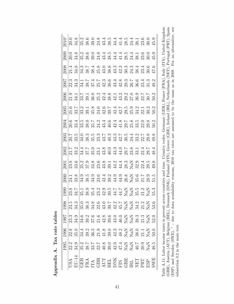
Appendix

A.Taxra

tetables

1995

1996

1997

1998

1999

2000

2001

2002

2003

2004

2005

2006

2007

2008

2009

2010

∗

USA

22.2

22.8

23.3

23.5

23.8

24.1

23.8

21.7

20.7

20.6

21.6

21.9

22.3

21.4

20.0

20.0

EU-14

34.9

35.0

34.9

34.3

34.7

33.8

33.6

33.2

33.5

33.4

33.7

34.1

34.3

34.8

34.8

34.8

GER

35.2

34.4

34.6

35.0

35.1

34.9

35.2

34.4

34.0

33.5

33.2

33.7

34.1

34.3

35.2

35.2

FRA

38.7

39.2

39.2

38.3

38.9

38.5

37.9

37.7

38.3

38.0

39.1

39.1

38.7

38.7

38.6

38.6

ITA

33.7

36.3

37.6

34.8

35.4

34.9

34.8

35.0

35.5

35.7

35.8

36.0

37.4

38.4

39.0

39.0

GBR

22.7

21.9

21.6

22.6

23.2

23.6

23.6

23.1

23.3

24.2

24.6

25.2

25.7

25.8

24.8

24.8

AUT

40.8

41.8

42.8

43.0

42.9

42.4

43.8

43.8

43.7

43.4

42.6

42.4

42.3

43.0

43.4

43.4

BEL

39.0

39.0

39.6

39.7

39.5

39.2

39.1

40.0

40.3

40.6

39.7

38.8

38.6

38.8

38.5

38.5

DNK

42.0

42.3

43.0

42.2

44.7

44.9

44.2

43.3

43.3

42.4

42.4

42.1

43.4

43.3

44.4

44.4

FIN

47.4

48.2

46.0

45.7

44.7

44.9

44.4

44.0

42.7

41.8

42.7

43.2

42.8

42.3

41.4

41.4

GRE

NaN

NaN

NaN

NaN

NaN

26.8

28.3

29.7

30.5

29.7

29.5

29.2

29.3

30.3

28.5

28.5

IRL

NaN

NaN

NaN

NaN

NaN

NaN

NaN

23.8

24.4

25.8

25.9

27.0

26.7

24.3

24.4

24.4

NET

40.7

38.0

38.3

34.2

35.5

35.6

32.9

33.1

33.2

33.5

34.2

36.9

36.6

38.4

38.1

38.1

PRT

20.9

21.1

21.3

21.2

21.2

21.7

22.4

22.4

22.7

22.0

22.1

22.7

23.4

23.4

23.6

23.6

ESP

NaN

NaN

NaN

NaN

NaN

28.9

29.5

29.7

29.8

29.8

30.2

30.7

31.3

30.6

30.0

30.0

SW

E48.5

50.0

52.0

53.6

55.3

51.5

49.8

48.4

49.8

50.2

50.2

50.2

48.2

47.6

45.9

45.9

Tab

leA.11:

Lab

orincometaxes

inpercentacross

countriesan

dtime.

Cou

ntrycodes:German

y(G

ER),France

(FRA),Italy(ITA),United

Kingdom

(GBR),Austria(A

UT),Belgium

(BEL),Denmark(D

NK),Finland(F

IN),Greece(G

RE),Irelan

d(IRL),Netherlands(N

ET),Portuga

l(P

RT),Spain

(ESP)and

Sweden

(SW

E).

∗-dueto

dataavailabilityreason

s,20

10taxratesareassumed

tobethesameas

in20

09.

For

analternative,

see

subsection3.2in

themaintext.

41

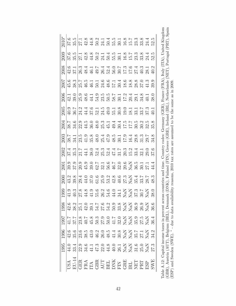
1995

1996

1997

1998

1999

2000

2001

2002

2003

2004

2005

2006

2007

2008

2009

2010

∗

USA

44.0

42.6

41.7

42.6

41.9

43.2

39.9

37.4

38.7

38.7

40.9

42.1

45.6

42.6

37.6

37.6

EU-14

33.4

35.6

37.7

38.2

40.3

39.8

37.9

35.3

34.1

34.6

36.7

39.0

38.3

37.1

35.5

35.5

GER

22.9

23.6

23.8

25.1

27.8

29.4

20.9

21.7

23.5

22.9

24.2

25.9

25.7

26.3

27.1

27.1

FRA

34.6

38.5

40.7

42.0

44.8

44.0

45.9

44.1

41.9

44.5

44.4

48.6

46.5

48.4

42.8

42.8

ITA

41.1

43.0

45.8

39.1

41.9

37.0

39.0

38.0

35.8

36.0

37.6

44.1

46.1

46.1

44.8

44.8

GBR

47.3

46.2

50.3

54.7

55.6

61.6

62.7

52.4

48.0

48.0

52.1

54.9

50.1

49.7

50.2

50.2

AUT

22.0

26.0

27.9

27.6

26.2

25.9

32.1

25.3

25.4

25.3

24.5

23.5

24.6

26.4

24.1

24.1

BEL

44.8

48.5

50.0

54.2

54.6

53.2

56.6

52.4

47.9

45.1

49.0

50.5

48.6

52.4

50.4

50.4

DNK

40.0

41.4

41.7

50.9

44.0

42.8

46.7

47.4

48.5

49.4

55.1

58.7

57.1

56.0

55.5

55.5

FIN

26.1

30.8

32.0

33.8

34.1

40.6

32.0

31.7

30.1

30.4

30.8

30.1

30.4

30.7

30.1

30.1

GRE

NaN

NaN

NaN

NaN

NaN

27.3

20.6

20.3

17.9

17.5

19.0

17.2

18.6

17.3

16.8

16.8

IRL

NaN

NaN

NaN

NaN

NaN

NaN

NaN

15.2

16.4

17.7

18.1

20.4

18.8

17.6

15.7

15.7

NET

31.6

35.7

35.9

36.9

37.3

35.4

36.5

33.4

29.8

30.5

33.1

29.1

28.8

27.4

23.3

23.3

PRT

25.0

27.1

27.5

26.9

30.7

33.7

30.1

32.1

31.3

30.2

33.7

34.8

37.0

40.3

33.8

33.8

ESP

NaN

NaN

NaN

NaN

NaN

28.7

27.1

29.0

29.7

32.5

37.3

40.1

41.3

28.1

24.4

24.4

SW

E27.3

34.2

36.4

36.6

38.0

48.3

44.4

37.6

34.8

35.8

40.1

38.0

39.9

40.2

52.5

52.5

Tab

leA.12:

Cap

ital

incometaxes

inpercentacross

countriesan

dtime.

Cou

ntrycodes:German

y(G

ER),France

(FRA),Italy(ITA),United

Kingdom

(GBR),Austria(A

UT),Belgium

(BEL),Denmark(D

NK),Finland(F

IN),Greece(G

RE),Irelan

d(IRL),Netherlands(N

ET),Portuga

l(P

RT),Spain

(ESP)andSweden

(SW

E).

∗-dueto

dataavailab

ilityreason

s,20

10taxratesareassumed

tobethesameas

in20

09.

42

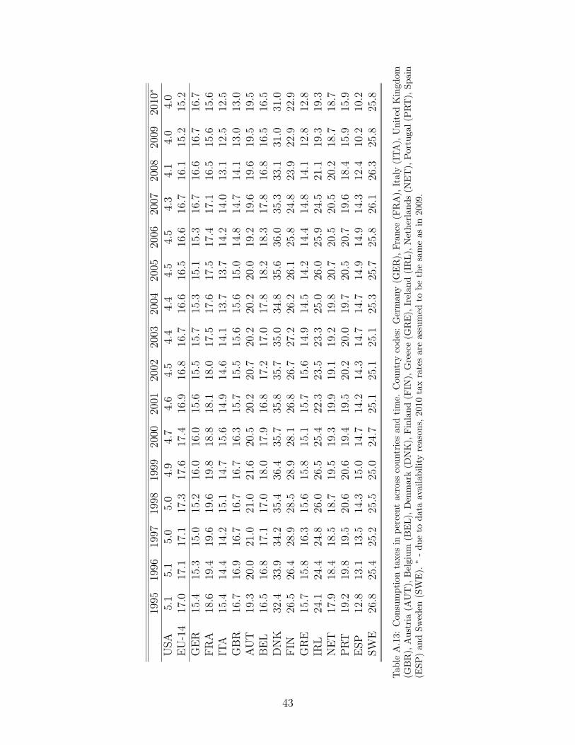
1995

1996

1997

1998

1999

2000

2001

2002

2003

2004

2005

2006

2007

2008

2009

2010

∗

USA

5.1

5.1

5.0

5.0

4.9

4.7

4.6

4.5

4.4

4.4

4.5

4.5

4.3

4.1

4.0

4.0

EU-14

17.0

17.1

17.1

17.3

17.6

17.4

16.9

16.8

16.7

16.6

16.5

16.6

16.7

16.1

15.2

15.2

GER

15.4

15.3

15.0

15.2

16.0

16.0

15.6

15.5

15.7

15.3

15.1

15.3

16.7

16.6

16.7

16.7

FRA

18.6

19.4

19.6

19.6

19.8

18.8

18.1

18.0

17.5

17.6

17.5

17.4

17.1

16.5

15.6

15.6

ITA

15.4

14.4

14.2

15.1

14.7

15.6

14.9

14.6

14.1

13.7

13.7

14.2

14.0

13.1

12.5

12.5

GBR

16.7

16.9

16.7

16.7

16.7

16.3

15.7

15.5

15.6

15.6

15.0

14.8

14.7

14.1

13.0

13.0

AUT

19.3

20.0

21.0

21.0

21.6

20.5

20.2

20.7

20.2

20.2

20.0

19.2

19.6

19.6

19.5

19.5

BEL

16.5

16.8

17.1

17.0

18.0

17.9

16.8

17.2

17.0

17.8

18.2

18.3

17.8

16.8

16.5

16.5

DNK

32.4

33.9

34.2

35.4

36.4

35.7

35.8

35.7

35.0

34.8

35.6

36.0

35.3

33.1

31.0

31.0

FIN

26.5

26.4

28.9

28.5

28.9

28.1

26.8

26.7

27.2

26.2

26.1

25.8

24.8

23.9

22.9

22.9

GRE

15.7

15.8

16.3

15.6

15.8

15.1

15.7

15.6

14.9

14.5

14.2

14.4

14.8

14.1

12.8

12.8

IRL

24.1

24.4

24.8

26.0

26.5

25.4

22.3

23.5

23.3

25.0

26.0

25.9

24.5

21.1

19.3

19.3

NET

17.9

18.4

18.5

18.7

19.5

19.3

19.9

19.1

19.2

19.8

20.7

20.5

20.5

20.2

18.7

18.7

PRT

19.2

19.8

19.5

20.6

20.6

19.4

19.5

20.2

20.0

19.7

20.5

20.7

19.6

18.4

15.9

15.9

ESP

12.8

13.1

13.5

14.3

15.0

14.7

14.2

14.3

14.7

14.7

14.9

14.9

14.3

12.4

10.2

10.2

SW

E26.8

25.4

25.2

25.5

25.0

24.7

25.1

25.1

25.1

25.3

25.7

25.8

26.1

26.3

25.8

25.8

Tab

leA.13:

Con

sumptiontaxes

inpercentacross

countriesan

dtime.

Cou

ntrycodes:German

y(G

ER),France

(FRA),Italy(ITA),United

Kingdom

(GBR),Austria(A

UT),Belgium

(BEL),Denmark(D

NK),Finland(F

IN),Greece(G

RE),Irelan

d(IRL),Netherlands(N

ET),Portuga

l(P

RT),Spain

(ESP)andSweden

(SW

E).

∗-dueto

dataavailab

ilityreason

s,20

10taxratesareassumed

tobethesameas

in20

09.

43

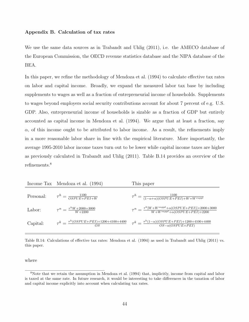
Appendix B. Calculation of tax rates

We use the same data sources as in Trabandt and Uhlig (2011), i.e. the AMECO database of

the European Commission, the OECD revenue statistics database and the NIPA database of the

BEA.

In this paper, we refine the methodology of Mendoza et al. (1994) to calculate effective tax rates

on labor and capital income. Broadly, we expand the measured labor tax base by including

supplements to wages as well as a fraction of entrepreneurial income of households. Supplements

to wages beyond employers social security contributions account for about 7 percent of e.g. U.S.

GDP. Also, entrepreneurial income of households is sizable as a fraction of GDP but entirely

accounted as capital income in Mendoza et al. (1994). We argue that at least a fraction, say

α, of this income ought to be attributed to labor income. As a result, the refinements imply

in a more reasonable labor share in line with the empirical literature. More importantly, the

average 1995-2010 labor income taxes turn out to be lower while capital income taxes are higher

as previously calculated in Trabandt and Uhlig (2011). Table B.14 provides an overview of the

refinements.8

Income Tax Mendoza et al. (1994) This paper

Personal: τh = 1100OSPUE+PEI+W

τh = 1100(1−α+α)(OSPUE+PEI)+W+W suppl

Labor: τn = τhW+2000+3000W+2200

τn = τh[W+W suppl+α(OSPUE+PEI)]+2000+3000W+W suppl+α(OSPUE+PEI)+2200

Capital: τ k = τh(OSPUE+PEI)+1200+4100+4400OS

τ k = τh(1−α)(OSPUE+PEI)+1200+4100+4400OS−α(OSPUE+PEI)

Table B.14: Calculations of effective tax rates: Mendoza et al. (1994) as used in Trabandt and Uhlig (2011) vs.this paper.

where

8Note that we retain the assumption in Mendoza et al. (1994) that, implicitly, income from capital and laboris taxed at the same rate. In future research, it would be interesting to take differences in the taxation of laborand capital income explicitly into account when calculating tax rates.

44

1100: Income, profit and capital gains taxes of individuals, revenue statistics (OECD).

1200: Income, profit and capital gains taxes of corporations, revenue statistics (OECD).

2000: Social security contributions, revenue statistics (OECD).

2200: Social security contributions of employers, revenue statistics (OECD).

3000: Payroll taxes, revenue statistics (OECD).

4000: Property taxes, revenue statistics (OECD).

4100: Recurrent taxes on immovable property, revenue statistics (OECD).

4400: Taxes on financial and capital transactions, revenue statistics (OECD).

OS: Net operating surplus: total economy (AMECO, NIPA).

W: Gross wages and salaries: households and NPISH (AMECO, NIPA).

OSPUE+PEI: Gross operating surplus minus consumption of fixed capital plus mixed income

plus net property income: households and NPISH (AMECO).

Wsuppl: Supplements to wages: households and NPISH. Calculated as the residual of compensa-

tion of employees minus wages and salaries minus social security contributions of employers.

We select a value for α such that the average 1995-2010 labor share, i.e. W+W suppl+α(OSPUE+

PEI)+2200)/GDP equals 64 percent in the U.S. It turns out that we need to set α = 0.35. We

keep the same value for α for all other countries.

Table B.15 shows the resulting effective tax rates across countries and compares them to those

when the standard Mendoza et al. (1994) methodology is applied as used e.g. in Trabandt and

Uhlig (2011). It turns out, that due to the broader labor tax base, effective labor taxes are

somewhat smaller while effective capital taxes are higher.

Finally, table B.16 provides maximum additional tax revenues that result from moving from

the peak of the Laffer curve when either the standard Mendoza et al. (1994) tax rates or the

refined version proposed in this paper are used. Further, the table also shows the implications

45

of imperfect vs. perfect competition. The introduction of imperfect competition reduces the

effective labor tax base and thus less additional tax revenues are attainable when varying labor

taxes. By contrast, profits arising from market power increase maximum additional tax revenues

when capital taxes are varied. The fourth column shows the results when the standard Mendoza

tax rates are used in the analysis and are essentially those obtained by Trabandt and Uhlig

(2011). In this case, higher effective labor taxes at the status quo equlibrium reduce the scope

for more tax revenues when labor and capital taxes are varied.

46

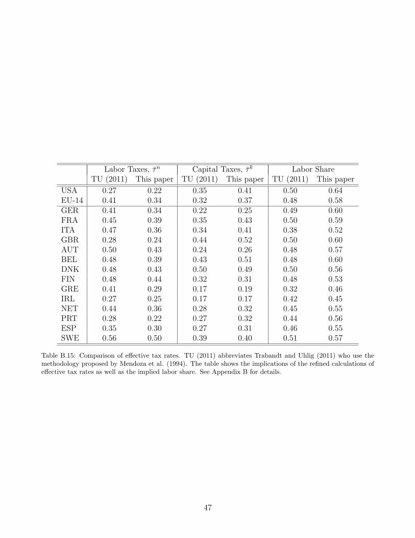
Labor Taxes, τn Capital Taxes, τ k Labor ShareTU (2011) This paper TU (2011) This paper TU (2011) This paper

USA 0.27 0.22 0.35 0.41 0.50 0.64EU-14 0.41 0.34 0.32 0.37 0.48 0.58GER 0.41 0.34 0.22 0.25 0.49 0.60FRA 0.45 0.39 0.35 0.43 0.50 0.59ITA 0.47 0.36 0.34 0.41 0.38 0.52GBR 0.28 0.24 0.44 0.52 0.50 0.60AUT 0.50 0.43 0.24 0.26 0.48 0.57BEL 0.48 0.39 0.43 0.51 0.48 0.60DNK 0.48 0.43 0.50 0.49 0.50 0.56FIN 0.48 0.44 0.32 0.31 0.48 0.53GRE 0.41 0.29 0.17 0.19 0.32 0.46IRL 0.27 0.25 0.17 0.17 0.42 0.45NET 0.44 0.36 0.28 0.32 0.45 0.55PRT 0.28 0.22 0.27 0.32 0.44 0.56ESP 0.35 0.30 0.27 0.31 0.46 0.55SWE 0.56 0.50 0.39 0.40 0.51 0.57

Table B.15: Comparison of effective tax rates. TU (2011) abbreviates Trabandt and Uhlig (2011) who use themethodology proposed by Mendoza et al. (1994). The table shows the implications of the refined calculations ofeffective tax rates as well as the implied labor share. See Appendix B for details.

47

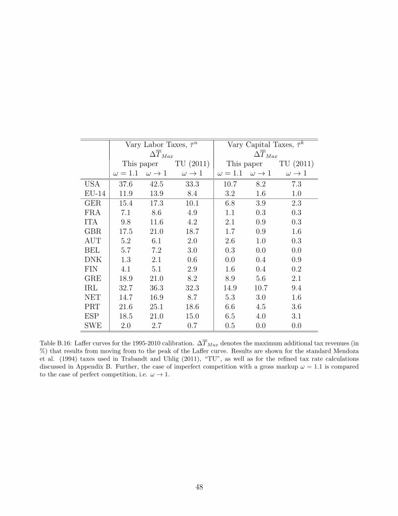
Vary Labor Taxes, τn Vary Capital Taxes, τ k

∆TMax ∆TMax

This paper TU (2011) This paper TU (2011)ω = 1.1 ω → 1 ω → 1 ω = 1.1 ω → 1 ω → 1

USA 37.6 42.5 33.3 10.7 8.2 7.3EU-14 11.9 13.9 8.4 3.2 1.6 1.0GER 15.4 17.3 10.1 6.8 3.9 2.3FRA 7.1 8.6 4.9 1.1 0.3 0.3ITA 9.8 11.6 4.2 2.1 0.9 0.3GBR 17.5 21.0 18.7 1.7 0.9 1.6AUT 5.2 6.1 2.0 2.6 1.0 0.3BEL 5.7 7.2 3.0 0.3 0.0 0.0DNK 1.3 2.1 0.6 0.0 0.4 0.9FIN 4.1 5.1 2.9 1.6 0.4 0.2GRE 18.9 21.0 8.2 8.9 5.6 2.1IRL 32.7 36.3 32.3 14.9 10.7 9.4NET 14.7 16.9 8.7 5.3 3.0 1.6PRT 21.6 25.1 18.6 6.6 4.5 3.6ESP 18.5 21.0 15.0 6.5 4.0 3.1SWE 2.0 2.7 0.7 0.5 0.0 0.0

Table B.16: Laffer curves for the 1995-2010 calibration. ∆TMax denotes the maximum additional tax revenues (in%) that results from moving from to the peak of the Laffer curve. Results are shown for the standard Mendozaet al. (1994) taxes used in Trabandt and Uhlig (2011), “TU”, as well as for the refined tax rate calculationsdiscussed in Appendix B. Further, the case of imperfect competition with a gross markup ω = 1.1 is comparedto the case of perfect competition, i.e. ω → 1.

48