
Housing Wealth E ects: The Long View - columbia.eduen2198/papers/longview.pdf · exploit systematic...
87
Housing Wealth Effects: The Long View Adam M. Guren * , Alisdair McKay † , Emi Nakamura ‡ , and J´ on Steinsson §¶ June 11, 2018 Abstract We provide new, time-varying estimates of the housing wealth effect back to the 1980s. We exploit systematic differences in city-level exposure to regional house price cycles to instru- ment for house prices. Our main findings are that: 1) Large housing wealth effects are not new: we estimate substantial effects back to the mid 1980s; 2) Housing wealth effects were not particularly large in the 2000s; if anything, they were larger prior to 2000; and 3) There is no evidence of a boom-bust asymmetry. We compare these findings to the implications of a standard life-cycle model with borrowing constraints, uninsurable income risk, illiquid housing, and long-term mortgages. The model explains our empirical findings about the insensitivity of the housing wealth effects to changes in the loan-to-value (LTV) distribution, including the dramatic rise in LTVs in the Great Recession. The insensitivity arises in the model for two reasons. First, impatient low-LTV agents have a high elasticity. Second, a rightward shift in the LTV distribution increases not only the number of highly sensitive constrained agents but also the number of underwater agents whose consumption is insensitive to house prices. * Boston University, [email protected] † Boston University, Federal Reserve Bank of Minneapolis, and NBER, [email protected] ‡ Columbia University and NBER, [email protected] § Columbia University and NBER [email protected] ¶ We would like to thank Massimiliano Cologgi, Hope Kerr, Jimmy Kuo, Jesse Silbert, Sergio Villar, and Xuiyi Song for excellent research assistance. We would like to thank Aditya Aladangady, Adrien Auclert, Masao Fukui, Peter Ganong, Dan Greenwald, Jonathon Hazell, Erik Hurst, Virgiliu Midrigan, Raven Molloy, Pascal Noel, Chris Palmer, Jonathan Parker, Monika Piazzesi, Esteban Rossi-Hansberg, Martin Schneider, Johannes Stroebel, Stijn Van Nieuwerburgh, Joseph Vavra, Gianluca Violante, Ivan Werning, and seminar participants at various institutions and conferences for useful comments. Guren thanks the National Science Foundation (grant SES-1623801) and the Boston University Center for Finance, Law, and Policy. Nakamura thanks the National Science Foundation (grant SES-1056107). Nakamura and Steinsson thank the Alfred P. Sloan Foundation for financial support. The views expressed herein are those of the authors and not necessarily those of the Federal Reserve Bank of Minneapolis or the Federal Reserve System.
Transcript of Housing Wealth E ects: The Long View - columbia.eduen2198/papers/longview.pdf · exploit systematic...
Housing Wealth Effects: The Long View
Adam M. Guren∗, Alisdair McKay†, Emi Nakamura‡, and Jon Steinsson§¶
June 11, 2018
Abstract
We provide new, time-varying estimates of the housing wealth effect back to the 1980s. We
exploit systematic differences in city-level exposure to regional house price cycles to instru-
ment for house prices. Our main findings are that: 1) Large housing wealth effects are not
new: we estimate substantial effects back to the mid 1980s; 2) Housing wealth effects were not
particularly large in the 2000s; if anything, they were larger prior to 2000; and 3) There is
no evidence of a boom-bust asymmetry. We compare these findings to the implications of a
standard life-cycle model with borrowing constraints, uninsurable income risk, illiquid housing,
and long-term mortgages. The model explains our empirical findings about the insensitivity
of the housing wealth effects to changes in the loan-to-value (LTV) distribution, including the
dramatic rise in LTVs in the Great Recession. The insensitivity arises in the model for two
reasons. First, impatient low-LTV agents have a high elasticity. Second, a rightward shift in
the LTV distribution increases not only the number of highly sensitive constrained agents but
also the number of underwater agents whose consumption is insensitive to house prices.
∗Boston University, [email protected]†Boston University, Federal Reserve Bank of Minneapolis, and NBER, [email protected]‡Columbia University and NBER, [email protected]§Columbia University and NBER [email protected]¶We would like to thank Massimiliano Cologgi, Hope Kerr, Jimmy Kuo, Jesse Silbert, Sergio Villar, and Xuiyi
Song for excellent research assistance. We would like to thank Aditya Aladangady, Adrien Auclert, Masao Fukui,Peter Ganong, Dan Greenwald, Jonathon Hazell, Erik Hurst, Virgiliu Midrigan, Raven Molloy, Pascal Noel, ChrisPalmer, Jonathan Parker, Monika Piazzesi, Esteban Rossi-Hansberg, Martin Schneider, Johannes Stroebel, StijnVan Nieuwerburgh, Joseph Vavra, Gianluca Violante, Ivan Werning, and seminar participants at various institutionsand conferences for useful comments. Guren thanks the National Science Foundation (grant SES-1623801) and theBoston University Center for Finance, Law, and Policy. Nakamura thanks the National Science Foundation (grantSES-1056107). Nakamura and Steinsson thank the Alfred P. Sloan Foundation for financial support. The viewsexpressed herein are those of the authors and not necessarily those of the Federal Reserve Bank of Minneapolis orthe Federal Reserve System.
1 Introduction
Housing wealth effects played an important role in both the boom of the early 2000s and the
recession that followed (Mian and Sufi, 2011; Mian, Rao and Sufi, 2013; Mian and Sufi, 2014). In
this paper, we ask whether large housing wealth effects were a special artifact of the 2000s boom-
bust cycle. It is often hypothesized that more households used their “houses as ATMs” in the 2000s
than before due to automated underwriting, expanded credit, and increased access to home equity
lines of credit (HELOCs). Moreover, household consumption may have been particularly responsive
to house price changes in the bust because the decline in house prices pushed an unusually large
number of households to high loan-to-value (LTV) ratios, causing borrowing constraints to bind.
While there is substantial existing evidence on housing wealth effects, particularly for the boom-
bust cycle of the 2000s, there is essentially no work that estimates whether housing wealth effects
have changed over time using a consistent empirical methodology.1
In this paper, we provide new, time-varying estimates of the housing wealth effect for the United
States using a consistent empirical methodology going back to the mid 1980s. We then use a stan-
dard model to evaluate our findings, and in doing so elucidate the mechanisms underlying the
housing wealth effect. While national house price cycles were much smaller early in our sample
than in the 2000s, there were substantial regional house price cycles. We exploit systematic differ-
ential exposure to these regional house price cycles across cities (formally, CBSAs) to identify our
estimates. Our baseline measure of the housing wealth effect is the elasticity of retail employment
per capita with respect to house prices, which we estimate using a 10-year rolling window panel
specification and a pooled panel specification.
We highlight three main empirical findings. First, large housing wealth effects are not new.
We estimate large effects back to the 1980s. Second, there is no evidence that housing wealth
effects were particularly large in the 2000s; if anything they were larger before 2000. Third, we
find no evidence of a boom-bust asymmetry that might arise from households hitting borrowing
constraints during housing busts. Our pooled estimate of the housing wealth effect for the sample
1To our knowledge, two papers have looked at changes over time. First, Case, Shiller, and Quigley (2013) find thatthe wealth effect was larger after 1986 than before using an OLS approach. Second, Aladangady (2017) finds thathousing wealth effects pre-2002 are not significantly different from post-2002, although his estimates are imprecise.Finally, by comparing Case, Shiller, and Quigley (2005), which uses data for 1982-1999, and Case, Shiller, and Quigley(2013), which covers 1978-2009 and has a higher estimate, one can attempt to back out the effect of adding the 2000s(along with 1978-82) to the sample. However, the two estimates are not in fact directly comparable, since boththe econometrics and data are different between the two papers. Other empirical estimates for the recent periodinclude Hurst and Stafford (2004); Campbell and Cocco (2007); Carroll, Otsuka, and Salacalek (2011), Attanasioet al. (2009, 2011), Calomiris, Longhofer, and Miles (2012), Cooper (2013); DeFusco (2016); Kaplan, Mitman, andViolante (2016), and Liebersohn (2017).
1
period 1990-2015 is an elasticity of 0.071, which is roughly equivalent to a marginal propensity to
consume out of housing wealth of 3.3 cents on the dollar.
To arrive at these estimates, we must confront several empirical challenges. House prices and
economic activity are jointly determined and causation can run in both directions. Moreover,
house prices are subject to substantial measurement error. The former concern is likely to impart
an upward bias on OLS estimates of the effect of house prices on retail employment, while the latter
concern will lead to a downward bias.
We confront these empirical challenges by developing what we refer to as a “sensitivity in-
strument” for changes in house prices. The basic idea is to interact an aggregate variable with
estimates of local exposure to this variable, as in the case of the well-known “Bartik instrument.”
We exploit the fact that house prices in some cities are systematically more sensitive to regional
house-price cycles than house prices in other cities. For example, when a house price boom occurs
in the Northeast region, Providence systematically experiences larger increases in house prices than
Rochester. Our panel data approach allows us to estimate the historical systematic sensitivity of
local house prices to regional housing cycles and construct an instrument by interacting the esti-
mated historical sensitivities with today’s shock to regional house prices. This simple approach
infers a housing wealth effect from the differential response of retail employment in Providence
relative to Rochester when the Northeast experiences a housing boom or bust. It overcomes both
measurement error concerns and endogeneity having to do with idiosyncratic local economic booms
(e.g., a large factory built in Providence for idiosyncratic reasons causes house prices to rise) under
the (strong) assumption of no city-level heterogeneity arising from non-housing sources.
We refine this simple approach by directly controlling for local and regional economic condi-
tions in the estimating equation for the local house price sensitivity parameters. This addresses
a “reverse causality” concern that house prices in Providence may be more sensitive to regional
house price cycles than house prices in Rochester because of differences in the cyclicality of the
local economy arising from non-housing sources. Our refined sensitivity instrument allows for city-
level heterogeneity arising from non-housing sources by exploiting only differences in the residual
sensitivity of house prices controlling for local economic conditions. Our panel data approach also
allows us to include a rich set of controls to account for other non-housing factors, including city
and region-time fixed effects, industry shares with time-specific coefficients, and differential local
sensitivities to aggregate variables that affect the housing market, such as risk premia and mortgage
interest rates. Our main identifying assumption is that conditional on these controls, there is no
2
unobserved factor that is both correlated with house prices in the time series and that differentially
affects the same cities that are more historically sensitive to regional housing cycles.
Three features of our empirical approach deserve emphasis. First, our approach does not rely
on aggregate house price variation being exogenous. In fact, aggregate house price variation can
be driven by the same shocks that drive aggregate retail employment, as suggested by recent work
in macroeconomics.2 Second, our sensitivity instrument is a powerful predictor of local house
prices: regional housing cycles explain roughly 40% of the variation in local house prices even after
controlling for local economic conditions. Third, our panel data approach based on data from
multiple house-price and macroeconomic cycles is much less sensitive to concerns about the Great
Recession being unusual in some way. This is the case because we observe previous recessions that
did not coincide with a large house price decline and previous house price changes that did not
coincide with a large recession.
Estimating the housing wealth effect by OLS yields a similar time-pattern as our baseline IV
specification. The OLS estimates are somewhat larger, presumably because of an upward bias due
to reverse causality. Recent work has used the Saiz (2010) instrument to estimate the housing
wealth effect (e.g., Mian and Sufi, 2011; Mian, Rao and Sufi, 2013; Mian and Sufi, 2014). When we
interact Saiz’s (2010) housing supply elasticity with a national house price shock, we continue to
find the same time series pattern as in our baseline results, but with significantly reduced precision.
We use retail employment as our main dependent variable, which we view as the best available
proxy for consumption that is both geographically disaggregated and available for a long sample
period. Retail employment comoves strongly with the BEA’s PCE measure of consumption at the
aggregate level. The BEA uses retail employment to impute local consumption in the regional
NIPA accounts, and private sector datasets do the same. Retail employment is also an important
component of non-tradable employment, which has been studied as a measure of local economic
activity (e.g., Mian and Sufi, 2014) and is of interest in its own right.3
Theoretically-minded readers may find it hard to interpret a “housing wealth effect.” House
prices are equilibrium variables that are affected by many shocks which may affect consumption
2The recent literature on general equilibrium models of house prices has emphasized shocks to current and expectedfuture productivity, credit constraints, and risk premia as plausible sources of variation in house prices Our empiricalanalysis is consistent with these being important sources of aggregate house price fluctuations (see, e.g. Landvoigt,Piazzesi, and Schneider, 2015; Favilukis, Ludvigson, and Van Nieuwerburgh, 2017; Kaplan, Mitman, and Violante,2017).
3The existing literature has looked at the effect of house prices on various economic outcomes, including bothconsumption and employment. Some studies focus on particular consumption categories such as consumer packagedgoods or cars (e.g., Mian and Sufi, 2011; Kaplan, Mitman, and Violante, 2016), while other studies have used morecomprehensive measures of consumption (e.g., Mian, Rao, and Sufi, 2013; Aladangady, 2017).
3
through other channels. So, what do our empirical estimates capture? In Section 5, we show
that in a simple general equilibrium model in which all markets are regional except for housing
markets, which are local, our empirical approach yields an estimate of the partial equilibrium effect
of house prices on consumption. In this case, both the direct effects of the shocks that drive
aggregate variation in house prices and all general equilibrium effects are soaked up by the region-
time fixed effects in our regressions. We also show that in a more realistic general equilibrium
model with segmented markets across cities, our empirical approach yields an estimate of the
partial equilibrium effect of house prices on consumption multiplied by a local general equilibrium
multiplier. We furthermore show that this local general equilibrium multiplier can be approximated
by estimates of the local fiscal multiplier (e.g., Nakamura and Steinsson, 2014).4 Since the recent
empirical literature estimates the local general equilibrium multiplier to be somewhat larger than
one, our estimate of the housing wealth effect is likely somewhat larger than the partial equilibrium
effect of house prices on consumption.
Recent research has greatly advanced our understanding of housing wealth effects in models
with uninsurable income shocks, borrowing constraints, illiquid housing, and long-term mortgages
(see, e.g., Agarwal et al., 2017; Berger et al., 2017; Chen, Michaux, and Roussanov, 2013; Davis and
Van Nieuwerburgh, 2015; Gorea and Midrigan, 2017; Guren, Krishnamurthy, and McQuade, 2018;
Kaplan, Mitman, and Violante, 2017; Li and Yao, 2007).5 In Sections 6 and 7, we lay out such a
model — which we refer to as the “new canonical model” of housing wealth effects — and confront
it with our empirical findings. We find that the model can generate a large housing wealth effect
and can explain the insensitivity of the housing wealth effect to the large changes in household
LTV ratios observed over our sample period and in particular during the Great Recession.
Two features of the model are important to understand these theoretical results. First, incom-
plete markets models of the type we analyze feature households that are impatient relative to the
interest rate. As a result, households have substantial marginal propensities to consume out of ex-
tra wealth even when they are not near their LTV constraint. This implies that a large fraction of
the housing wealth effect in our model is due to the large number of households that have relatively
low LTV ratios. Furthermore, because low LTV households have a strong housing wealth effect,
the effect does not get substantially stronger as LTVs rise.
4This formalizes intuitive arguments made by Mian and Sufi (2015).5Earlier theoretical research suggested that the housing wealth effect might be zero because increased wealth from
higher house prices was offset by higher implicit costs of living (Sinai and Souleles, 2005). This stark conclusionresults from several simplifying assumptions including complete markets and households that live in the same houseforever.
4
Second, in our model, households with negative equity are insensitive to changes in house prices.
In the presence of long-term debt, underwater households are not forced to de-lever to meet an
LTV constraint and, furthermore, are unable to sell their house without an equity injection. Since
these households cannot access changes in housing equity that result from increases in house prices,
they are largely unresponsive to these changes, as Ganong and Noel (2017) have emphasized. As a
consequence, the large rightward shift in the LTV distribution that resulted from the fall in prices
during the 2007-2010 housing bust had two offsetting effects on the housing wealth effect. On the
one hand, more households were pushed closer to their LTV constraint and consequently became
more sensitive to changes in house prices. On the other hand, more households became underwater
on their mortgage to the point that they became insensitive to changes in house prices. In our
model, these two effects roughly offset to deliver a relatively stable elasticity in the Great Recession
despite a large rightward shift in the LTV distribution.
Some may find it surprising to learn that households were spending out of their home equity a
quarter century ago. However, the main tools used to extract housing equity — such as cash-out
refinancing and HELOCs — have been available for several decades, and the HELOC share of
mortgage debt only rose from 7 percent to 9 percent in the 2000s boom according to the Flow of
Funds. Mortgage securitization was invented in the late 1960s and has been done on a large scale
since the late 1970s. Others have argued that the major changes in mortgage debt availability
occurred in the 1970s (see, e.g., Kuhn, Schularick, and Steins, 2017; Foote, Gerardi, and Willen,
2012). While certain mortgage products may have become available in the 2000s to segments of
the population that did not have access to them before, our model shows that this is not likely
to have materially affected the overall housing wealth effect. The following quote from Townsend-
Greenspan’s August 1982 client report written by Alan Greenspan illustrates well how much access
households had to housing equity even before the start of our sample period:
The combination of very rapidly rising prices for existing homes and a sharp increase
in sales ... of these homes has created a huge increase in capital gains and purchasing
power during the past two years ... by far the greater part has been drawn out of home
equities and spent on other goods and services or put into savings. In fact, of the more
than $60 billion ... increase in the market value of existing homes ... virtually the entire
amount was monetized as mortgage debt extensions, creating nearly a 5% increase in
consumer purchasing power.
5
A modern reader might be excused for thinking that this paragraph was written by Greenspan
circa 2005.6
The paper proceeds as follows. Section 2 describes our main data sources. Section 3 describes
our empirical methodology. Section 4 describes our empirical results. Section 5 makes explicit the
link between our empirical analysis and the theoretical analysis that follows. Section 6 presents
our partial equilibrium model. Section 7 analyzes how changes in household balance sheets affect
the housing wealth effect in the model. Section 8 concludes.
2 Data
To estimate the housing wealth effect, we need a measure of local economic activity and a measure
of house prices. Our main measure of local economic activity is retail employment per capita. Retail
employment has long been viewed by measurement agencies as one of the best available proxies
for consumer expenditures. For example, BEA’s Regional PCE measures and the private sector
“Survey of Buying Power” both use retail employment data to impute consumer expenditures in
between economic census years.
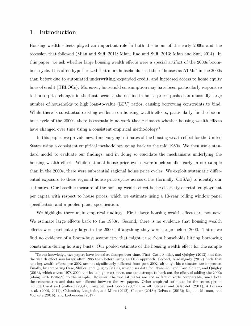
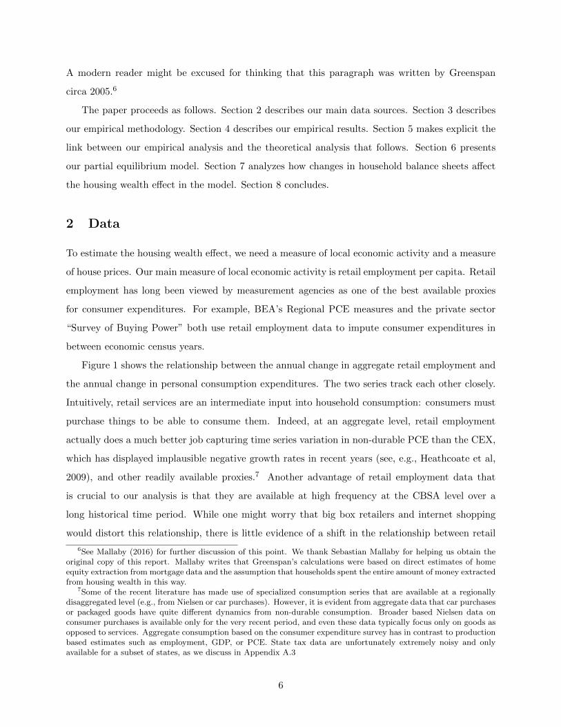
Figure 1 shows the relationship between the annual change in aggregate retail employment and
the annual change in personal consumption expenditures. The two series track each other closely.
Intuitively, retail services are an intermediate input into household consumption: consumers must
purchase things to be able to consume them. Indeed, at an aggregate level, retail employment
actually does a much better job capturing time series variation in non-durable PCE than the CEX,
which has displayed implausible negative growth rates in recent years (see, e.g., Heathcoate et al,
2009), and other readily available proxies.7 Another advantage of retail employment data that
is crucial to our analysis is that they are available at high frequency at the CBSA level over a
long historical time period. While one might worry that big box retailers and internet shopping
would distort this relationship, there is little evidence of a shift in the relationship between retail
6See Mallaby (2016) for further discussion of this point. We thank Sebastian Mallaby for helping us obtain theoriginal copy of this report. Mallaby writes that Greenspan’s calculations were based on direct estimates of homeequity extraction from mortgage data and the assumption that households spent the entire amount of money extractedfrom housing wealth in this way.
7Some of the recent literature has made use of specialized consumption series that are available at a regionallydisaggregated level (e.g., from Nielsen or car purchases). However, it is evident from aggregate data that car purchasesor packaged goods have quite different dynamics from non-durable consumption. Broader based Nielsen data onconsumer purchases is available only for the very recent period, and even these data typically focus only on goods asopposed to services. Aggregate consumption based on the consumer expenditure survey has in contrast to productionbased estimates such as employment, GDP, or PCE. State tax data are unfortunately extremely noisy and onlyavailable for a subset of states, as we discuss in Appendix A.3
6
−6
−4
−2
02
4%
Ch
an
ge
Fro
m Y
ea
r A
go
1985 1995 2005 2015Date
Retail Emp Real PCE
Figure 1: Growth of Retail Employment vs. Growth in Personal Consumption Expenditures
Note: The figure plots the 4-quarter change in aggregate retail employment (FRED series CEU4200000001) and the4-quarter aggregate change in real personal consumption expenditures (FRED series PCECC96). We take out alinear time trend from both series to account for trend growth.
employment and PCE in Figure 1. Furthermore, our main specification is in first differences and
includes time fixed effects, so our estimates are not affected by smooth trends or growth rates.
In Appendix A.3 we analyze the relationship between city-level consumption and retail em-
ployment using data for 17 cities for which the BLS publishes city-level consumption using data
from the Consumer Expenditure Survey. Both the CEX and retail employment have substantial
sampling error. We use an instrumental variables approach to correct for measurement error in
retail employment per capita. Once we address measurement error, consumer expenditures respond
nearly one-for-one with to retail employment per capita.8
Our data for retail employment comes from the Quarterly Census of Employment and Wages
(QCEW) which is available back to 1975 at the county level. The population data come from the
Census Bureau’s post-Censal population estimates for 1970 to 2010 and inter-Censal population
estimates for 2010 to 2017. These estimates are available annually, and we interpolate to a quarterly
8We have also verified, in unreported work, that changes in CBSA-level retail employment are highly correlatedwith changes in retail sales over the 5-year intervals at which retail sales are available in the Economic Census.
7
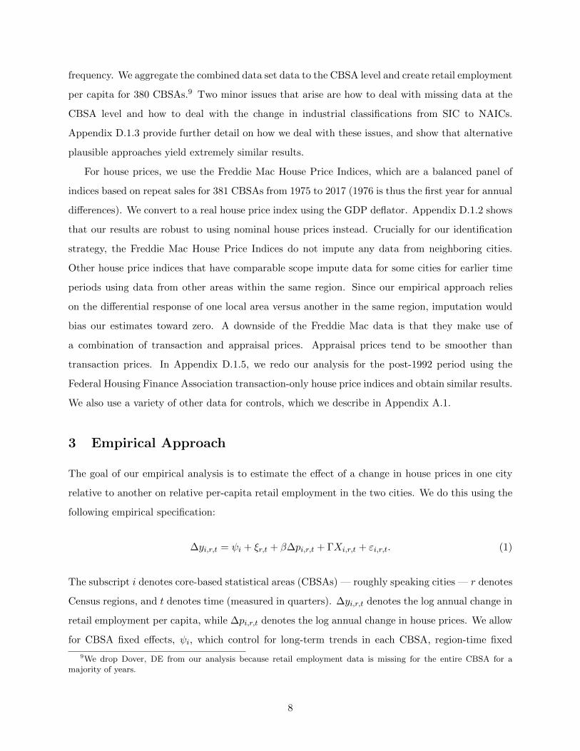
frequency. We aggregate the combined data set data to the CBSA level and create retail employment
per capita for 380 CBSAs.9 Two minor issues that arise are how to deal with missing data at the
CBSA level and how to deal with the change in industrial classifications from SIC to NAICs.
Appendix D.1.3 provide further detail on how we deal with these issues, and show that alternative
plausible approaches yield extremely similar results.
For house prices, we use the Freddie Mac House Price Indices, which are a balanced panel of
indices based on repeat sales for 381 CBSAs from 1975 to 2017 (1976 is thus the first year for annual
differences). We convert to a real house price index using the GDP deflator. Appendix D.1.2 shows
that our results are robust to using nominal house prices instead. Crucially for our identification
strategy, the Freddie Mac House Price Indices do not impute any data from neighboring cities.
Other house price indices that have comparable scope impute data for some cities for earlier time
periods using data from other areas within the same region. Since our empirical approach relies
on the differential response of one local area versus another in the same region, imputation would
bias our estimates toward zero. A downside of the Freddie Mac data is that they make use of
a combination of transaction and appraisal prices. Appraisal prices tend to be smoother than
transaction prices. In Appendix D.1.5, we redo our analysis for the post-1992 period using the
Federal Housing Finance Association transaction-only house price indices and obtain similar results.
We also use a variety of other data for controls, which we describe in Appendix A.1.
3 Empirical Approach
The goal of our empirical analysis is to estimate the effect of a change in house prices in one city
relative to another on relative per-capita retail employment in the two cities. We do this using the
following empirical specification:
∆yi,r,t = ψi + ξr,t + β∆pi,r,t + ΓXi,r,t + εi,r,t. (1)
The subscript i denotes core-based statistical areas (CBSAs) — roughly speaking cities — r denotes
Census regions, and t denotes time (measured in quarters). ∆yi,r,t denotes the log annual change in
retail employment per capita, while ∆pi,r,t denotes the log annual change in house prices. We allow
for CBSA fixed effects, ψi, which control for long-term trends in each CBSA, region-time fixed
9We drop Dover, DE from our analysis because retail employment data is missing for the entire CBSA for amajority of years.
8

effects, ξr,t, which imply that our effects are identified only off of differential movements across
CBSAs within a region, a set of additional controls, Xi,r,t, and other unmodeled influences on retail
employment, εi,r,t.
The coefficient of interest in equation (1) is β, which measures the housing wealth effect as
an elasticity. Several challenges arise in estimating β. Causation runs both ways between local
employment and house prices, implying that the error term in equation (1) will be correlated
with the change in house prices. This is likely to bias OLS estimates of β upward since a strong
economy will cause house prices to rise. On the other hand, house prices are measured with
error, potentially biasing β towards zero. To address these two sources of bias, we propose a new
instrumental variables strategy for estimating β. Our instrument leverages systematic differences
in the sensitivity of local house prices to aggregate shocks across CBSAs.
3.1 Simple Intuition for Identification
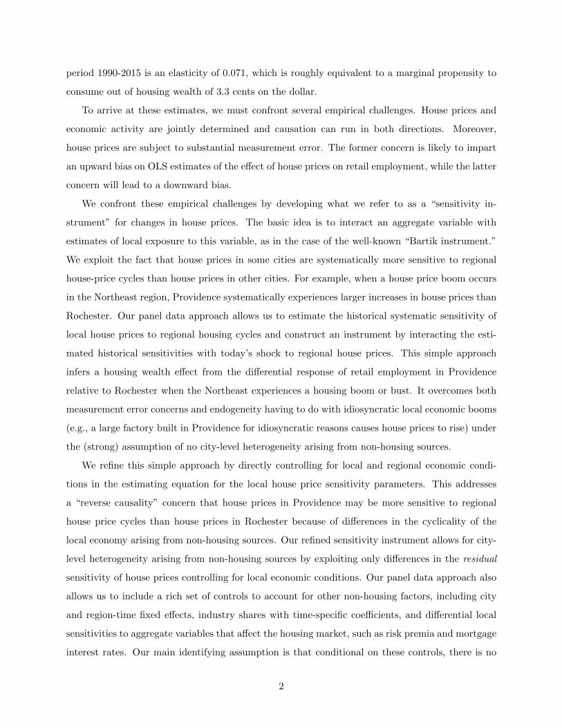
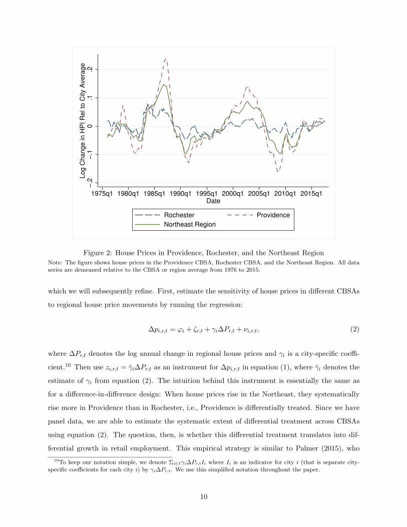
Before developing our identification strategy in detail, it is useful to consider an example. Figure
2 plots the time series of house prices in Providence and Rochester as well as the Northeast region
as a whole. Two features of this example are important for our identification strategy. First,
house prices in the Northeast have experienced large regional boom-bust cycles throughout our
sample period. In particular, there was a large house-price cycle in the Northeast in the 1980s in
addition to the house-price cycle of the 2000s. Regional house price cycles like the 1980s cycle in
the Northeast occurred in several regions of the U.S. in the 1980s and 1990s. The timing of these
regional cycles has varied, and they largely averaged out for the nation as a whole except for the
nationwide boom-bust cycle of the 2000s. The existence of these regional cycles helps us estimate
the housing wealth effect before 2000 when identification strategies using nation-wide variation in
house prices lose power.
Second, the sensitivity of house prices in different CBSAs in the Northeast to the regional
house price cycle varies systematically. When house prices boom in the Northeast, house prices
in Providence respond much more than house prices in Rochester. This pattern of differential
sensitivity is stable over the entire sample period, as noted by Sinai (2013). Furthermore, this
pattern is a pervasive feature of house price data across different CBSAs and regions. A likely
reason for this differential sensitivity is variation in current and future expected housing supply
constraints. We discuss this in more detail below.
These two features of house price dynamics suggest the following simple identification strategy,
9
−.2
−.1
0.1
.2L
og
Ch
an
ge
in
HP
I R
el to
City A
ve
rag
e
1975q1 1980q1 1985q1 1990q1 1995q1 2000q1 2005q1 2010q1 2015q1Date
Rochester Providence
Northeast Region
Figure 2: House Prices in Providence, Rochester, and the Northeast Region
Note: The figure shows house prices in the Providence CBSA, Rochester CBSA, and the Northeast Region. All dataseries are demeaned relative to the CBSA or region average from 1976 to 2015.
which we will subsequently refine. First, estimate the sensitivity of house prices in different CBSAs
to regional house price movements by running the regression:
∆pi,r,t = ϕi + ζr,t + γi∆Pr,t + νi,r,t, (2)
where ∆Pr,t denotes the log annual change in regional house prices and γi is a city-specific coeffi-
cient.10 Then use zi,r,t = γi∆Pr,t as an instrument for ∆pi,r,t in equation (1), where γi denotes the
estimate of γi from equation (2). The intuition behind this instrument is essentially the same as
for a difference-in-difference design: When house prices rise in the Northeast, they systematically
rise more in Providence than in Rochester, i.e., Providence is differentially treated. Since we have
panel data, we are able to estimate the systematic extent of differential treatment across CBSAs
using equation (2). The question, then, is whether this differential treatment translates into dif-
ferential growth in retail employment. This empirical strategy is similar to Palmer (2015), who
10To keep our notation simple, we denote Σi∈Iγi∆Pr,tIi where Ii is an indicator for city i (that is separate city-specific coefficients for each city i) by γi∆Pr,t. We use this simplified notation throughout the paper.
10
instruments for house prices in the Great Recession using the historical variance of a city’s house
prices interacted with the national change in house prices.
3.2 Refined Identification Strategy
The simple procedure described above runs into problems if retail employment responds differ-
entially to regional shocks through other channels than local house prices. Suppose, for example,
that there are differences in industrial structure across CBSAs that induce differences in the cyclical
sensitivity of employment to the aggregate business cycle (for reasons other than housing). In this
case, the heterogeneity in γi may arise from reverse causality.11 This, in turn, would lead to biased
estimates of β.
To address this problem, we refine the procedure described above for estimating γi by controlling
for local and regional changes in retail employment allowing the coefficients on these variables to
vary across CBSAs:
∆pi,r,t = ϕi + δi∆yi,r,t + µi∆Yr,t + γi∆Pr,t + ΨXi,r,t + νi,r,t, (3)
where Xi,r,t are additional controls. We exclude the CBSA in question from the construction of
the regional house price index when running this regression, so as to avoid bias in γi due to the
same price being on both the left and right hand side.12 We also estimate equation (3) using time
periods other than the time period for which we are estimating equation (1). We do this to avoid
γi reflecting endogenous variation in local house prices over the period we are estimating equation
(1). For the rolling window estimates in section 4, we use all time periods outside a given 10-year
window in estimating our rolling window coefficients. In the pooled estimates across time periods,
we construct the instrument for each year using data excluding a 3 year buffer around the time
period in question. In practice, these different leave-out procedures yield similar results.
As before, zi,r,t = γi∆Pr,t is the instrument we propose to use for ∆pi,r,t in equation (1). This
instrument captures the portion of local house price variation that is explained by differential
11Suppose, for example, that Providence has an industrial structure tilted towards highly cyclical durable goodsrelative to Rochester. In this case, a positive aggregate demand shock would lead retail employment to increasemore in Providence than Rochester. If local economic booms raise house prices, this would induce a larger change inhouse prices in Providence than Rochester and, thus, imply that we would estimate a higher γi for Providence usingequation (2) purely due to reverse causality.
12There is an arithmetic reason not to include region-time fixed effects in equation 3 that arises as a consequence ofthis leave-out procedure. Since a leave-out mean appears in this regression, arithmetically, it is possible to perfectlypredict local house prices if region-time fixed effects are included.
11
sensitivity to the regional house price index holding ∆yi,r,t and ∆Yr,t fixed. For this approach to
yield a powerful instrument, there must be substantial variation in house prices that is orthogonal
to movements in local and regional retail employment. This is the case in our data: when we run
regression (3) without the differential sensitivity term γi∆Pr,t, the R-squared is 0.18, but when
γi∆Pr,t is added, the R-squared rises to 0.62. In other words, our sensitivity instrument explains
a large fraction of the total variation in local house prices, even conditioning on local and regional
employment.13
The key identifying assumption in our analysis is that, conditional on controls, there are no
other aggregate factors that are both correlated with regional house prices in the time series and
that differentially impact retail employment per capita in the same CBSAs that are sensitive to
house prices as captured by γi. In other words, to bias our results there must exist a confounding
factor with the structure αiEr,t where Er,t is correlated with regional house prices in the time series
and αi is correlated with γi in the cross section. Appendix C presents a more formal discussion of
our identifying assumptions in the context of a two-equation simultaneous equations system from
which we explicitly derive our estimating equations.
Our instrument is a close cousin of the Bartik instrument, which instruments for city labor
demand by summing across industries the share of an industry in each city multiplied by the
national change in employment in that industry. These two instruments are, in turn, close cousins
of difference-in-difference designs. The crucial idea in all of these strategies is that certain locations
are differentially treated by an aggregate shock. For example, consider a Bartik instrument in
which the key source of variation is differential exposure to oil shocks in Texas versus Florida. The
identifying assumption is that there is not some other factor that happens to differentially affect
Texas at the same time as oil prices go up. Our identifying assumption that there is no aggregate
factor that is correlated with regional house prices in the time series and that differentially impacts
retail employment in a way correlated with γi has a similar flavor.
In thinking about the validity of these strategies, it is important to understand that treatment
intensity (in our case γi and in the case of the Bartik instrument the industry shares) need not be
randomly assigned. This is in fact rarely the case. In the Bartik example, Texas and Florida obvi-
13One potential concern with this procedure is the role of measurement error in ∆yi,r,t biasing the δi terms andthereby creating bias in the γis. To assess the severity of this concern, we have also considered a specification inwhich we instrument for ∆yi,r,t using a 2-digit Bartik instrument for local economic conditions. For power reasons,we must assume that δi is the same across CSBAs, but the δ we obtain is a causal elasticity. We obtain an estimatefor δ of 2.9. This estimate for δ can be used to subtract δ∆yi,r,t from ∆pi,r,t, and then we can use this adjusted∆pi,r,t to estimate γi. This approach yields values for the γi that are highly correlated with our baseline approach,and using these alternate γis does not significantly alter our results.
12
ously differ in other ways than just their exposure to oil shocks, but as long as the key identification
assumption holds, this does not in and of itself invalidate the instrument.
An important advantage of estimating β using a panel specification is that we can control for
differential sensitivity of local retail employment to observable aggregate variables. This allows us
to rule out many potential confounding factors with a αiEr,t structure. First, we control for local
industry shares with separate coefficients for each time period. This accounts for all differential
factors that are correlated in the cross-section with industry structure. For example, this accounts
for differential labor demand across cities, as with the original “Bartik” instrument. It also accounts
for differential city-level exposure to unobservable risk premia associated with industrial structure.
For example, this control would capture unobservables relating to some cities having more risky
industries than others and therefore being differentially affected by shocks to risk aversion. Second,
we include separate controls for the differential city-level exposure to regional retail employment,
real 30-year mortgage rates, and Gilchirst and Zakrajek’s (2012) measure of bond risk premia. For
each of these, we construct the control in an analogous fashion to our instrument by estimating an
OLS regression:
∆yi,r,t = ψi + ξr,t + αi∆Xr,t + εi,r,t, (4)
where ∆X is either the log change in regional retail employment, the change in the 30-year fixed
mortgage rate, or the change of the Gilchirst-Zakrajek excess bond premium. We then include each
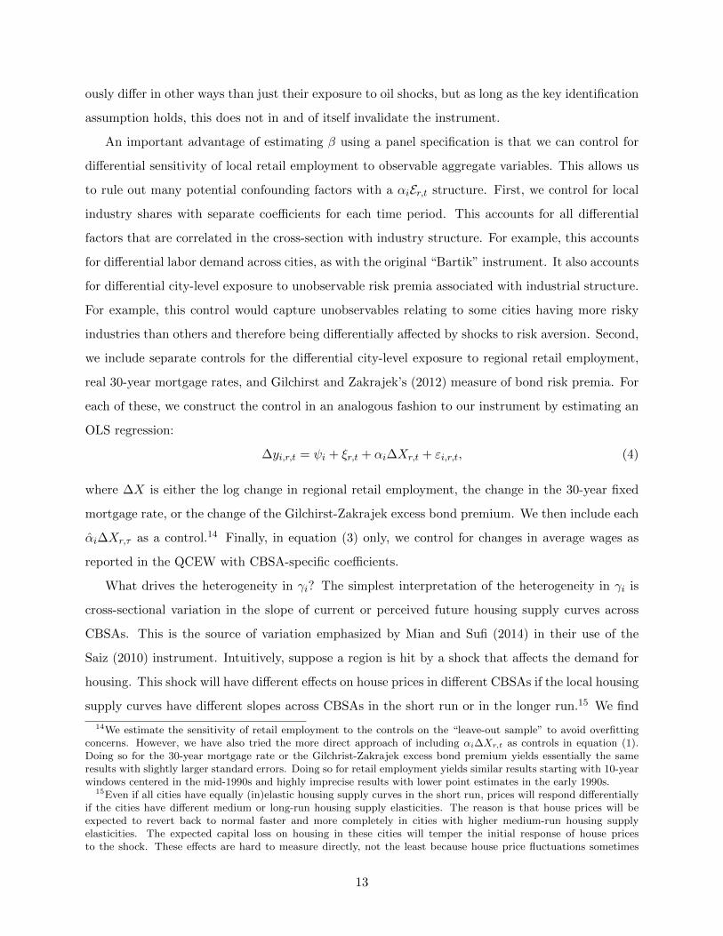
αi∆Xr,τ as a control.14 Finally, in equation (3) only, we control for changes in average wages as
reported in the QCEW with CBSA-specific coefficients.
What drives the heterogeneity in γi? The simplest interpretation of the heterogeneity in γi is
cross-sectional variation in the slope of current or perceived future housing supply curves across
CBSAs. This is the source of variation emphasized by Mian and Sufi (2014) in their use of the
Saiz (2010) instrument. Intuitively, suppose a region is hit by a shock that affects the demand for
housing. This shock will have different effects on house prices in different CBSAs if the local housing
supply curves have different slopes across CBSAs in the short run or in the longer run.15 We find
14We estimate the sensitivity of retail employment to the controls on the “leave-out sample” to avoid overfittingconcerns. However, we have also tried the more direct approach of including αi∆Xr,t as controls in equation (1).Doing so for the 30-year mortgage rate or the Gilchrist-Zakrajek excess bond premium yields essentially the sameresults with slightly larger standard errors. Doing so for retail employment yields similar results starting with 10-yearwindows centered in the mid-1990s and highly imprecise results with lower point estimates in the early 1990s.
15Even if all cities have equally (in)elastic housing supply curves in the short run, prices will respond differentiallyif the cities have different medium or long-run housing supply elasticities. The reason is that house prices will beexpected to revert back to normal faster and more completely in cities with higher medium-run housing supplyelasticities. The expected capital loss on housing in these cities will temper the initial response of house pricesto the shock. These effects are hard to measure directly, not the least because house price fluctuations sometimes
13
that the R-squared of univariate regressions of our estimates of γi over the full sample on Saiz’s
housing supply elasticity is 17%, on Saiz’s land unavailability index is 14%, and on the Wharton
Land Use Regulation Index is 16%. Regressing our γi’s on all three of these measures together
yields an R-squared of 23%. One advantage of our instrument versus the Saiz instrument is that
there are likely to be many sources of variation in housing supply elasticities beyond those based
on physical geography. These include land use regulation (Saiz, 2010) and future housing supply
constraints (Nathanson and Zwick, 2017). Some regions may also be more “bubbly,” perhaps due
to social connections to inelastic cities (Bailey et al., 2017) or credit (Favara and Imbs, 2015). Our
instrument will capture all these sources of variation. This implies that it is substantially more
powerful than the Saiz instrument. Also, our instrument can be calculated for any geographical
area, while the Saiz instrument is available only for 269 Metropolitan Statistical Areas.
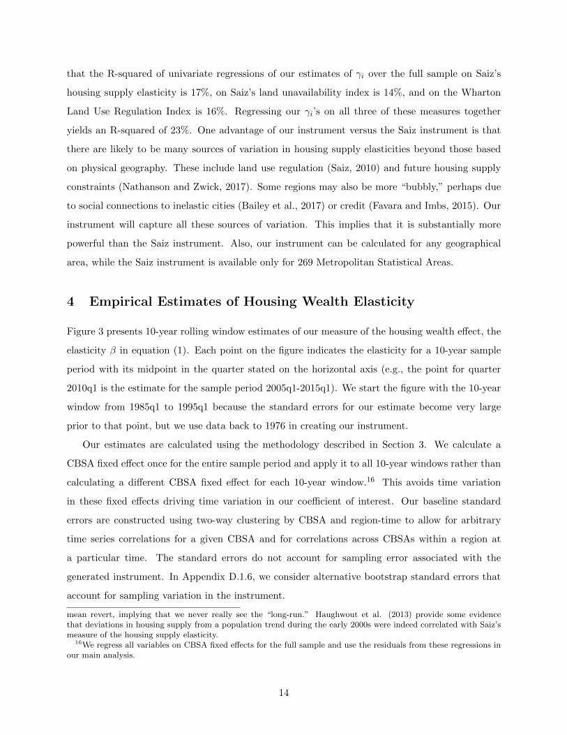
4 Empirical Estimates of Housing Wealth Elasticity
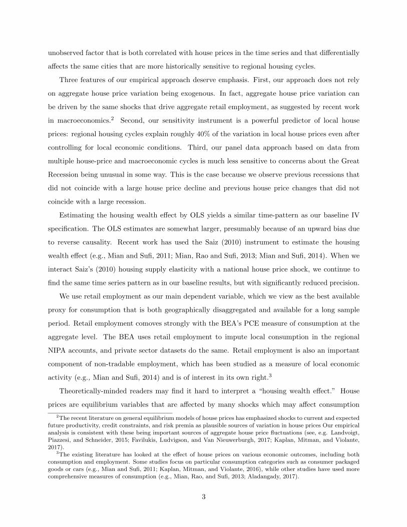
Figure 3 presents 10-year rolling window estimates of our measure of the housing wealth effect, the
elasticity β in equation (1). Each point on the figure indicates the elasticity for a 10-year sample
period with its midpoint in the quarter stated on the horizontal axis (e.g., the point for quarter
2010q1 is the estimate for the sample period 2005q1-2015q1). We start the figure with the 10-year
window from 1985q1 to 1995q1 because the standard errors for our estimate become very large
prior to that point, but we use data back to 1976 in creating our instrument.
Our estimates are calculated using the methodology described in Section 3. We calculate a
CBSA fixed effect once for the entire sample period and apply it to all 10-year windows rather than
calculating a different CBSA fixed effect for each 10-year window.16 This avoids time variation
in these fixed effects driving time variation in our coefficient of interest. Our baseline standard
errors are constructed using two-way clustering by CBSA and region-time to allow for arbitrary
time series correlations for a given CBSA and for correlations across CBSAs within a region at
a particular time. The standard errors do not account for sampling error associated with the
generated instrument. In Appendix D.1.6, we consider alternative bootstrap standard errors that
account for sampling variation in the instrument.
mean revert, implying that we never really see the “long-run.” Haughwout et al. (2013) provide some evidencethat deviations in housing supply from a population trend during the early 2000s were indeed correlated with Saiz’smeasure of the housing supply elasticity.
16We regress all variables on CBSA fixed effects for the full sample and use the residuals from these regressions inour main analysis.
14
−.1
0.1
.2IV
Ela
sticity o
f R
eta
il E
mp to H
ouse P
rices
1990q1 1995q1 2000q1 2005q1 2010q1Midpoint of 10 Year Window
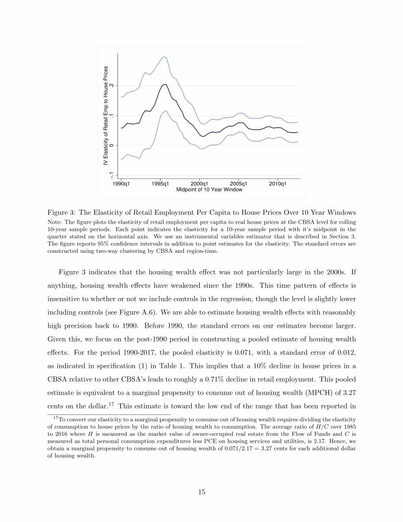
Figure 3: The Elasticity of Retail Employment Per Capita to House Prices Over 10 Year Windows
Note: The figure plots the elasticity of retail employment per capita to real house prices at the CBSA level for rolling10-year sample periods. Each point indicates the elasticity for a 10-year sample period with it’s midpoint in thequarter stated on the horizontal axis. We use an instrumental variables estimator that is described in Section 3.The figure reports 95% confidence intervals in addition to point estimates for the elasticity. The standard errors areconstructed using two-way clustering by CBSA and region-time.
Figure 3 indicates that the housing wealth effect was not particularly large in the 2000s. If
anything, housing wealth effects have weakened since the 1990s. This time pattern of effects is
insensitive to whether or not we include controls in the regression, though the level is slightly lower
including controls (see Figure A.6). We are able to estimate housing wealth effects with reasonably
high precision back to 1990. Before 1990, the standard errors on our estimates become larger.
Given this, we focus on the post-1990 period in constructing a pooled estimate of housing wealth
effects. For the period 1990-2017, the pooled elasticity is 0.071, with a standard error of 0.012,
as indicated in specification (1) in Table 1. This implies that a 10% decline in house prices in a
CBSA relative to other CBSA’s leads to roughly a 0.71% decline in retail employment. This pooled
estimate is equivalent to a marginal propensity to consume out of housing wealth (MPCH) of 3.27
cents on the dollar.17 This estimate is toward the low end of the range that has been reported in
17To convert our elasticity to a marginal propensity to consume out of housing wealth requires dividing the elasticityof consumption to house prices by the ratio of housing wealth to consumption. The average ratio of H/C over 1985to 2016 where H is measured as the market value of owner-occupied real estate from the Flow of Funds and C ismeasured as total personal consumption expenditures less PCE on housing services and utilities, is 2.17. Hence, weobtain a marginal propensity to consume out of housing wealth of 0.071/2.17 = 3.27 cents for each additional dollarof housing wealth.
15
−.0
50
.05
Log C
hange in H
PI R
esid
ualiz
ed
−.1 −.05 0 .05 .1Instrument Residualized
First Stage
−.0
04
−.0
02
0.0
02
.004
Log C
hange in R
eta
il E
mp R
esid
ualiz
ed
−.1 −.05 0 .05 .1Instrument Residualized
Reduced Form
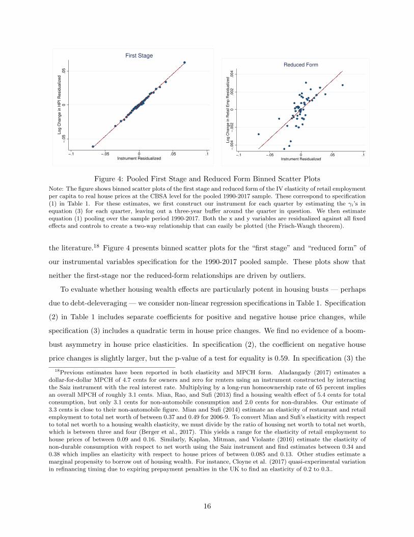
Figure 4: Pooled First Stage and Reduced Form Binned Scatter Plots
Note: The figure shows binned scatter plots of the first stage and reduced form of the IV elasticity of retail employmentper capita to real house prices at the CBSA level for the pooled 1990-2017 sample. These correspond to specification(1) in Table 1. For these estimates, we first construct our instrument for each quarter by estimating the γi’s inequation (3) for each quarter, leaving out a three-year buffer around the quarter in question. We then estimateequation (1) pooling over the sample period 1990-2017. Both the x and y variables are residualized against all fixedeffects and controls to create a two-way relationship that can easily be plotted (the Frisch-Waugh theorem).
the literature.18 Figure 4 presents binned scatter plots for the “first stage” and “reduced form” of
our instrumental variables specification for the 1990-2017 pooled sample. These plots show that
neither the first-stage nor the reduced-form relationships are driven by outliers.
To evaluate whether housing wealth effects are particularly potent in housing busts — perhaps
due to debt-deleveraging — we consider non-linear regression specifications in Table 1. Specification
(2) in Table 1 includes separate coefficients for positive and negative house price changes, while
specification (3) includes a quadratic term in house price changes. We find no evidence of a boom-
bust asymmetry in house price elasticities. In specification (2), the coefficient on negative house
price changes is slightly larger, but the p-value of a test for equality is 0.59. In specification (3) the
18Previous estimates have been reported in both elasticity and MPCH form. Aladangady (2017) estimates adollar-for-dollar MPCH of 4.7 cents for owners and zero for renters using an instrument constructed by interactingthe Saiz instrument with the real interest rate. Multiplying by a long-run homeownership rate of 65 percent impliesan overall MPCH of roughly 3.1 cents. Mian, Rao, and Sufi (2013) find a housing wealth effect of 5.4 cents for totalconsumption, but only 3.1 cents for non-automobile consumption and 2.0 cents for non-durables. Our estimate of3.3 cents is close to their non-automobile figure. Mian and Sufi (2014) estimate an elasticity of restaurant and retailemployment to total net worth of between 0.37 and 0.49 for 2006-9. To convert Mian and Sufi’s elasticity with respectto total net worth to a housing wealth elasticity, we must divide by the ratio of housing net worth to total net worth,which is between three and four (Berger et al., 2017). This yields a range for the elasticity of retail employment tohouse prices of between 0.09 and 0.16. Similarly, Kaplan, Mitman, and Violante (2016) estimate the elasticity ofnon-durable consumption with respect to net worth using the Saiz instrument and find estimates between 0.34 and0.38 which implies an elasticity with respect to house prices of between 0.085 and 0.13. Other studies estimate amarginal propensity to borrow out of housing wealth. For instance, Cloyne et al. (2017) quasi-experimental variationin refinancing timing due to expiring prepayment penalties in the UK to find an elasticity of 0.2 to 0.3..
16
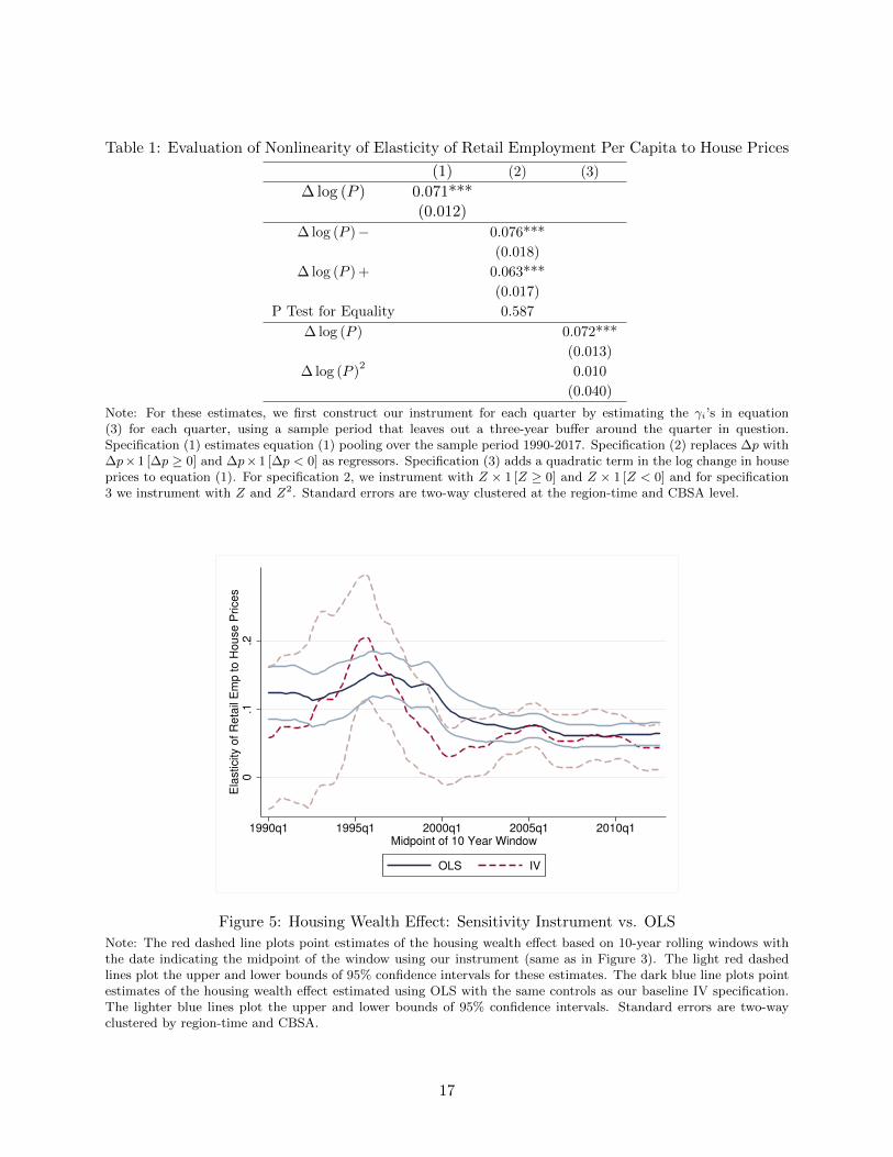
Table 1: Evaluation of Nonlinearity of Elasticity of Retail Employment Per Capita to House Prices
(1) (2) (3)
∆ log (P ) 0.071***(0.012)
∆ log (P )− 0.076***
(0.018)
∆ log (P ) + 0.063***
(0.017)
P Test for Equality 0.587
∆ log (P ) 0.072***
(0.013)
∆ log (P )2
0.010
(0.040)
Note: For these estimates, we first construct our instrument for each quarter by estimating the γi’s in equation(3) for each quarter, using a sample period that leaves out a three-year buffer around the quarter in question.Specification (1) estimates equation (1) pooling over the sample period 1990-2017. Specification (2) replaces ∆p with∆p×1 [∆p ≥ 0] and ∆p×1 [∆p < 0] as regressors. Specification (3) adds a quadratic term in the log change in houseprices to equation (1). For specification 2, we instrument with Z × 1 [Z ≥ 0] and Z × 1 [Z < 0] and for specification3 we instrument with Z and Z2. Standard errors are two-way clustered at the region-time and CBSA level.
0.1
.2E
lasticity o
f R
eta
il E
mp to H
ouse P
rices
1990q1 1995q1 2000q1 2005q1 2010q1Midpoint of 10 Year Window
OLS IV
Figure 5: Housing Wealth Effect: Sensitivity Instrument vs. OLS
Note: The red dashed line plots point estimates of the housing wealth effect based on 10-year rolling windows withthe date indicating the midpoint of the window using our instrument (same as in Figure 3). The light red dashedlines plot the upper and lower bounds of 95% confidence intervals for these estimates. The dark blue line plots pointestimates of the housing wealth effect estimated using OLS with the same controls as our baseline IV specification.The lighter blue lines plot the upper and lower bounds of 95% confidence intervals. Standard errors are two-wayclustered by region-time and CBSA.
17
0.2
5.5
IV E
lasticity o
f R
eta
il E
mp to H
ouse P
rices
1990q1 1995q1 2000q1 2005q1 2010q1Midpoint of 10 Year Window
Saiz Sensitivity Instrument
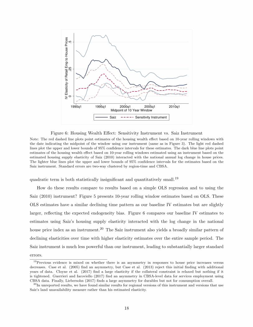
Figure 6: Housing Wealth Effect: Sensitivity Instrument vs. Saiz Instrument
Note: The red dashed line plots point estimates of the housing wealth effect based on 10-year rolling windows withthe date indicating the midpoint of the window using our instrument (same as in Figure 3). The light red dashedlines plot the upper and lower bounds of 95% confidence intervals for these estimates. The dark blue line plots pointestimates of the housing wealth effect based on 10-year rolling windows estimated using an instrument based on theestimated housing supply elasticity of Saiz (2010) interacted with the national annual log change in house prices.The lighter blue lines plot the upper and lower bounds of 95% confidence intervals for the estimates based on theSaiz instrument. Standard errors are two-way clustered by region-time and CBSA.
quadratic term is both statistically insignificant and quantitatively small.19
How do these results compare to results based on a simple OLS regression and to using the
Saiz (2010) instrument? Figure 5 presents 10-year rolling window estimates based on OLS. These
OLS estimates have a similar declining time pattern as our baseline IV estimates but are slightly
larger, reflecting the expected endogeneity bias. Figure 6 compares our baseline IV estimates to
estimates using Saiz’s housing supply elasticity interacted with the log change in the national
house price index as an instrument.20 The Saiz instrument also yields a broadly similar pattern of
declining elasticities over time with higher elasticity estimates over the entire sample period. The
Saiz instrument is much less powerful than our instrument, leading to substantially larger standard
errors.
19Previous evidence is mixed on whether there is an asymmetry in responses to house price increases versusdecreases. Case et al. (2005) find an asymmetry, but Case et al. (2013) reject this initial finding with additionalyears of data. Cloyne et al. (2017) find a large elasticity if the collateral constraint is relaxed but nothing if itis tightened. Guerrieri and Iacoviello (2017) find an asymmetry in CBSA-level data for services employment usingCBSA data. Finally, Liebersohn (2017) finds a large asymmetry for durables but not for consumption overall.
20In unreported results, we have found similar results for regional versions of this instrument and versions that useSaiz’s land unavailability measure rather than his estimated elasticity.
18
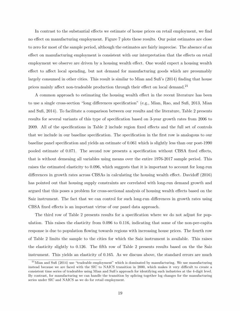
In contrast to the substantial effects we estimate of house prices on retail employment, we find
no effect on manufacturing employment. Figure 7 plots these results. Our point estimates are close
to zero for most of the sample period, although the estimates are fairly imprecise. The absence of an
effect on manufacturing employment is consistent with our interpretation that the effects on retail
employment we observe are driven by a housing wealth effect. One would expect a housing wealth
effect to affect local spending, but not demand for manufacturing goods which are presumably
largely consumed in other cities. This result is similar to Mian and Sufi’s (2014) finding that house
prices mainly affect non-tradeable production through their effect on local demand.21
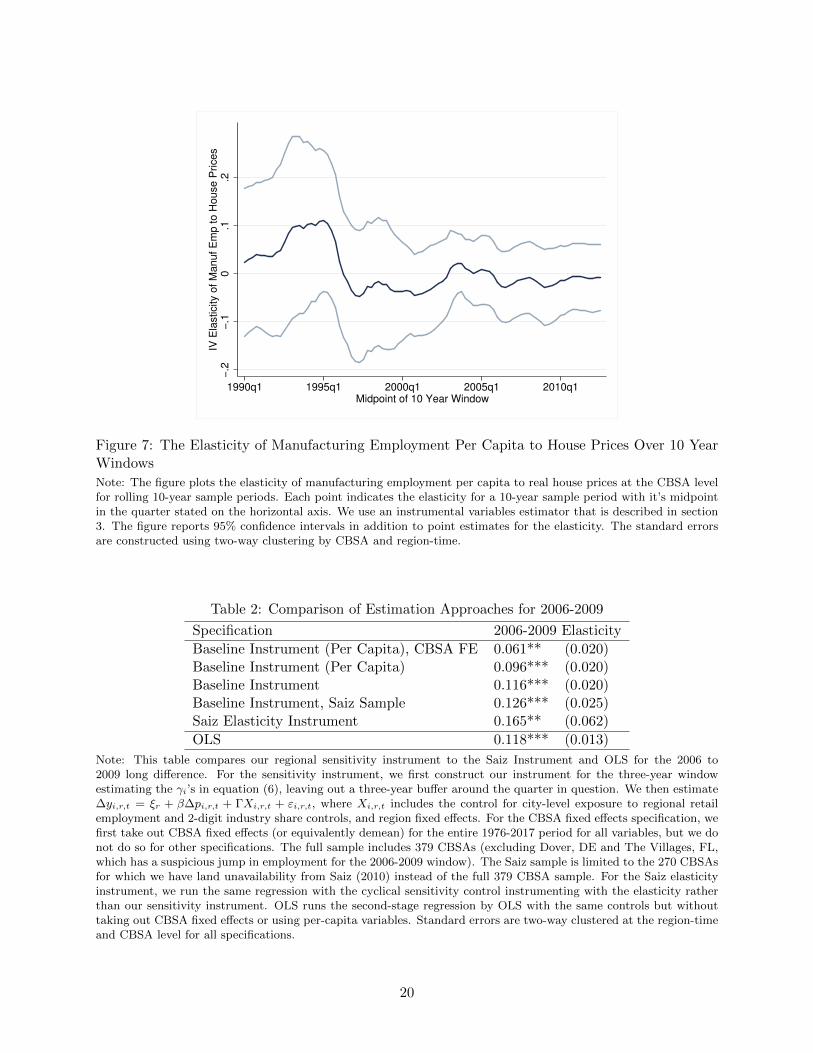
A common approach to estimating the housing wealth effect in the recent literature has been
to use a single cross-section “long differences specification” (e.g., Mian, Rao, and Sufi, 2013, Mian
and Sufi, 2014). To facilitate a comparison between our results and the literature, Table 2 presents
results for several variants of this type of specification based on 3-year growth rates from 2006 to
2009. All of the specifications in Table 2 include region fixed effects and the full set of controls
that we include in our baseline specification. The specification in the first row is analogous to our
baseline panel specification and yields an estimate of 0.061 which is slightly less than our post-1990
pooled estimate of 0.071. The second row presents a specification without CBSA fixed effects,
that is without demeaing all variables using means over the entire 1976-2017 sample period. This
raises the estimated elasticity to 0.096, which suggests that it is important to account for long-run
differences in growth rates across CBSAs in calculating the housing wealth effect. Davidoff (2016)
has pointed out that housing supply constraints are correlated with long-run demand growth and
argued that this poses a problem for cross-sectional analysis of housing wealth effects based on the
Saiz instrument. The fact that we can control for such long-run differences in growth rates using
CBSA fixed effects is an important virtue of our panel data approach.
The third row of Table 2 presents results for a specification where we do not adjust for pop-
ulation. This raises the elasticity from 0.096 to 0.116, indicating that some of the non-per-capita
response is due to population flowing towards regions with increasing house prices. The fourth row
of Table 2 limits the sample to the cities for which the Saiz instrument is available. This raises
the elasticity slightly to 0.126. The fifth row of Table 2 presents results based on the the Saiz
instrument. This yields an elasticity of 0.165. As we discuss above, the standard errors are much
21Mian and Sufi (2014) use “tradeable employment” which is dominated by manufacturing. We use manufacturinginstead because we are faced with the SIC to NAICS transition in 2000, which makes it very difficult to create aconsistent time series of tradeables using Mian and Sufi’s approach for identifying such industries at the 4-digit level.By contrast, for manufacturing we can handle the transition by splicing together log changes for the manufacturingseries under SIC and NAICS as we do for retail employment.
19
−.2
−.1
0.1
.2IV
Ela
sticity o
f M
anuf E
mp to H
ouse P
rices
1990q1 1995q1 2000q1 2005q1 2010q1Midpoint of 10 Year Window
Figure 7: The Elasticity of Manufacturing Employment Per Capita to House Prices Over 10 YearWindows
Note: The figure plots the elasticity of manufacturing employment per capita to real house prices at the CBSA levelfor rolling 10-year sample periods. Each point indicates the elasticity for a 10-year sample period with it’s midpointin the quarter stated on the horizontal axis. We use an instrumental variables estimator that is described in section3. The figure reports 95% confidence intervals in addition to point estimates for the elasticity. The standard errorsare constructed using two-way clustering by CBSA and region-time.
Table 2: Comparison of Estimation Approaches for 2006-2009
Specification 2006-2009 Elasticity
Baseline Instrument (Per Capita), CBSA FE 0.061** (0.020)Baseline Instrument (Per Capita) 0.096*** (0.020)Baseline Instrument 0.116*** (0.020)Baseline Instrument, Saiz Sample 0.126*** (0.025)Saiz Elasticity Instrument 0.165** (0.062)
OLS 0.118*** (0.013)
Note: This table compares our regional sensitivity instrument to the Saiz Instrument and OLS for the 2006 to2009 long difference. For the sensitivity instrument, we first construct our instrument for the three-year windowestimating the γi’s in equation (6), leaving out a three-year buffer around the quarter in question. We then estimate∆yi,r,t = ξr + β∆pi,r,t + ΓXi,r,t + εi,r,t, where Xi,r,t includes the control for city-level exposure to regional retailemployment and 2-digit industry share controls, and region fixed effects. For the CBSA fixed effects specification, wefirst take out CBSA fixed effects (or equivalently demean) for the entire 1976-2017 period for all variables, but we donot do so for other specifications. The full sample includes 379 CBSAs (excluding Dover, DE and The Villages, FL,which has a suspicious jump in employment for the 2006-2009 window). The Saiz sample is limited to the 270 CBSAsfor which we have land unavailability from Saiz (2010) instead of the full 379 CBSA sample. For the Saiz elasticityinstrument, we run the same regression with the cyclical sensitivity control instrumenting with the elasticity ratherthan our sensitivity instrument. OLS runs the second-stage regression by OLS with the same controls but withouttaking out CBSA fixed effects or using per-capita variables. Standard errors are two-way clustered at the region-timeand CBSA level for all specifications.
20
larger when using the Saiz instrument. The final row of Table 2 presents results based on OLS,
which yields an elasticity of 0.118. As with our main results, our sensitivity instrument gives lower
estimates of housing wealth elasticities than OLS, while the Saiz instrument gives higher estimates
than OLS.
5 Data to Theory
In the decision problem of a household, house prices are exogenous. The “causal effect” of house
prices on household consumption in such a partial equilibrium setting is therefore straightforward to
interpret. By contrast, at the aggregate level or city level, house prices are an endogenous variable.
House prices are affected by a myriad of shocks and these shocks may affect consumption not only
through house prices but also directly or through other channels. So what does it mean to estimate
the causal effect of house prices on consumption at the city level?
Consider a simple model of an economy consisting of several regions with many cities in each
region. Suppose housing markets are local to each city and the cities differ in their housing supply
elasticities. All other markets are fully integrated across cities within a region (and may in some
cases be integrated across regions). The cities are initially in identical steady states before being hit
by a one-time, unexpected, and permanent aggregate shock that alters the demand for housing. This
shock leads house prices to respond differently across cities due to the difference in housing supply
elasticities, but all other prices respond symmetrically within region because all other markets are
integrated within region. It is not important for our argument exactly what the nature of the
aggregate shock is. It could be an aggregate productivity shock, and aggregate demand shock (e.g.,
monetary, fiscal, or news shock), or an aggregate housing specific shock such as a shock to the
preference for housing or to construction costs.
Consumption in city i, in region r, and at time t can be written as ci,r,t = c(pi,r,t, ωi,r,t,Ωr,t, Rr,t),
where ωi,r,t is a vector of idiosyncratic shocks, Ωr,t is a vector of regional or national shocks, Rr,t
is a vector of prices such as interest rates and wages. One can interpret Rr,t as including not only
current prices, but also prices for future-dated goods. Since all markets other than the housing
market are integrated across cities within region, Rr,t does not have an i subscript. All cities have
the same aggregate consumption function. Consumption only differs across cities to the extent that
they experience different home prices and different shocks. In an Online Supplement, we provide
an example of a fully-specified general-equilibrium model that of the type described above that
21
yields a consumption function of this form.22
Take a log-linear approximation to the aggregate consumption function around the initial steady
state and then take an annual difference. This yields:
∆ci,r,t = φp︸︷︷︸β
∆pi,r,t + φΩ∆Ωr,t + φR∆Rr,t︸ ︷︷ ︸ξr,t
+φω∆ωi,r,t︸ ︷︷ ︸εi,r,t
, (5)
where ci,r,t denotes the logarithm of consumption and φx denotes the elasticity of c(· · · ) with respect
to the variable x evaluated at the steady state. These elasticities should be understood as vectors
of elasticities where appropriate. Equation (5) is labeled to show how it relates to equation (1) in
our empirical analysis.
Suppose we ran the empirical specification described in Section 3 on data from this model.
Equation (5) shows that the general equilibrium impact of changes in prices other than house prices
as well as the direct effect of aggregate and regional shocks will be absorbed by the region-time
fixed effects ξr,t. Our coefficient of interest β captures the response of consumption to a house price
change holding these other variables constant. This shows that if we are able to identify variation
in local house prices that is orthogonal to the error terms ξr,t and εi,r,t and the assumptions stated
above about market structure hold, the coefficient β will estimate the partial equilibrium effect of
house prices on consumption.23
The simple general equilibrium model discussed above makes the strong assumption that all
markets except the housing market are fully integrated across cities within a region. If we relax this
assumption, the differential response of house prices across cities will result in differential responses
in other markets as well. In other words, the differential house price movements will result in
local general equilibrium effects. Since these local general equilibrium effects will differ across
cities within a region, they will not be absorbed by the region-time fixed effects in our empirical
specification and will affect our estimate of β.
Local general equilibrium effects result from changes in local demand affecting local wages,
prices, and incomes. This suggests that evidence from other local demand shocks might be useful
in pinning down the effect of local general equilibrium on our empirical estimates. In the Online
22The Online Supplement can be found at http://people.bu.edu/guren/gmnsPEtoGE.pdf .23If non-linearities are important, the fixed effects in equation (5) will not fully absorb the general equilibrium
price effects. For example, if consumption growth responds importantly to ∆pi,r,t × ∆Ωr,t or to ∆pi,r,t × ∆Rr,t,then our estimated β will reflect these interactions in addition to the housing wealth effect. In the next section wepresent a fully non-linear model of the housing wealth effect and we show in Appendix E.1 that the model impliesthese interaction effects are small. In particular, the housing wealth effect is close to linear in the magnitude of theprice change and symmetric with respect to positive and negative price changes.
22
Supplement, we present a general-equilibrium regional business cycle model with heterogeneous
housing supply elasticities that allows for local general equilibrium effects. In this model, we show
that the local government spending multiplier can be used to quantify local general equilibrium
effects. More specifically, we show that the housing wealth effect estimate β that results from our
empirical specification can be expressed as:
β ' βLFMβPE ,
where βLFM denotes the local fiscal multiplier and βPE denotes the partial equilibrium effect of
house prices on consumption.24 Intuitively, a dollar of spending triggers the same local general
equilibrium response regardless of whether it arises from a housing wealth effect or government
spending. Nakamura and Steinsson (2014) estimate that the local government spending multiplier
is roughly 1.5 at the state level but 1.8 at the region level. Since our analysis is at the CBSA level,
the relevant local government spending multiplier for our analysis is likely somewhat smaller than
1.5.
6 A Model of the Local Consumption Response to House Prices
We now present our version of the new canonical model of housing and consumption. The key
features of the model are a life cycle, uninsured idiosyncratic income risk, borrowing constraints,
illiquid housing, and long-term mortgage debt subject to an LTV constraint. We keep our model
purposefully simple and evaluate its robustness to some of our starker assumptions in Appendix E.
6.1 Assumptions
Households live for T periods and have preferences over non-durable consumption and housing
services given by,
E0
[T∑t=1
βtu(ct, ht+1) + βT+1B(wT+1)
],
24We make certain simplifying assumptions to derive this result. One of these is to assume GHH preferences toavoid wealth effects on labor supply. We abstract from the collateral channel emphasized by Chaney, Sraer, andThesmar (2012) and Adelino, Schoar, and Severino (2015). We assume that the government and households bothbuy the same consumption good. Finally, we assume that construction employment does not respond to house prices.In the Online Supplement, we assess how relaxing this last assumption affects our results.
23
where c is consumption, h is housing, B(·) is a bequest motive, and wT+1 is the wealth of offspring.
We parameterize household preferences as:
u(c, h) =1
1− γ
(c(ε−1)/ε + ωh(ε−1)/ε
)(1−γ)ε/(ε−1)
B(w) =B0
1− γ(w +B1)(1−γ) .
Here γ captures the curvature of the utility function, ε is the elasticity of substitution between
housing and non-durable consumption, B0 captures the strength of the warm-glow bequest motive,
and B1 captures non-homotheticity in bequest motives.25
An individual can consume housing either by owning or renting. A unit of housing can be
purchased at price p or rented for one period at cost δp. This implies that the rent-price ratio is
fixed and given by the parameter δ. We make this simplifying assumption to avoid counter-factual
flows between renting and owning in response to changes in house prices. We consider alternative
assumptions about the behavior of rents in Appendix E. In our baseline model, people expect home
prices will remain at their current level. Renting h units of housing delivers the same utility as
buying that amount of housing, but the rent is more expensive than the user cost of owner occupied
housing, which makes owning attractive despite its associated transaction costs. To sell a house
the individual must pay ψSell of the value of the house in a transaction cost and to buy a house
the individual must pay ψBuy.
Households can take out mortgages. We denote the mortgage principal that a household brings
into the period by m. At origination, mortgage debt must satisfy,
m′ ≤ θph′, (6)
where θ is the maximum LTV and primes denote next period values. The mortgage interest rate
is Rm and a household must pay a transaction cost of ψmm′ to originate a mortgage. We model
mortgages as long-term debt that households can refinance at any time. To refinance, a household
must pay the same transaction cost as when a mortgage is initiated (ψmm′ where m′ is the new
mortgage balance). The repayment schedule requires a payment such that m′ = G(a)Rmm, where
a is the age of the household. Following Campbell and Cocco (2003), G(a) is defined so that the
25In the presence of illiquid durable goods such as housing, the parameter γ is related to, but not equivalent to,the coefficient of risk aversion (see Flavin and Nakagawa, 2008).
24
loan amortizes over the rest of the homeowner’s lifetime. The amortization schedule is given by:
G(a) ≡ 1− 1−R−1m
1−R−(T−a+1)m
.
The household can save, but not borrow, in liquid assets with return Ra < Rm. Finally, we
model log annual income as log y = `+ z + ξ, where ` is a deterministic life-cycle component, z is
a persistent shock that follows an AR(1) process, and ξ is a transitory shock.
6.2 Calibration
A household is born at age 25, works for 36 years, retiring at 61, and dies deterministically after
age 80. We set most of the parameters through external calibration, which we describe first, and
then we set a small set of parameters through internal calibration. We set the curvature of the
utility function, γ, to 2. We set the elasticity of substitution between housing and non-durable
consumption to 1.25 based on the estimates of Piazzesi, Schneider, and Tuzel (2007). We set the
LTV limit, θ, to 0.80 based on GSE guidelines for conforming mortgages without private mortgage
insurance. We set the after-tax, real interest rate on mortgage debt to 3 percent per year based on
the long-run averages of nominal mortgage rates and inflation.26 We set the real return on liquid
assets to 1 percent based on the difference between the long-run averages of the 1-year Treasury
rate and inflation. We set the cost of buying a house to 2 percent. This is meant to reflect closing
costs associated with a home purchase.
During the household’s working years, we model log annual income as the sum of a life-cycle
component, a transitory component, and a persistent component. The life-cycle component is taken
from Guvenen et al. (2016). We conceive of the transitory income shocks as non-employment shocks
motivated by the income process in Guvenen et al. (2016). With some probability the household
is employed for the full year and the (log) transitory income shock is zero. With the remaining
probability, the household spends part of the year out of work. The fraction of the year the
household spends non-employed is drawn from an exponential distribution truncated to the interval
(0, 1). The probability of a non-zero non-employment shock and the parameter of the exponential
distribution are estimated by maximum likelihood using the distribution of weeks worked in the
prior year reported in the 2002 March CPS. The persistent component of labor income is modeled
26Between 1971 and 2017 the average CPI inflation rate was 4.1 percent, the average 30-year fixed rate mortgagerate was 8.2 percent, and the average 1-year treasury rate was 5.3 percent. Our choice of a 3 percent real interestrate on mortgage debt is meant to capture the tax-deductibility of mortgage interest.
25
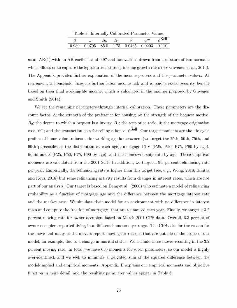
Table 3: Internally Calibrated Parameter Values
β ω B0 B1 δ ψm ψSell
0.939 0.0795 85.0 1.75 0.0435 0.0203 0.110
as an AR(1) with an AR coefficient of 0.97 and innovations drawn from a mixture of two normals,
which allows us to capture the leptokurtic nature of income growth rates (see Guvenen et al., 2016).
The Appendix provides further explanation of the income process and the parameter values. At
retirement, a household faces no further labor income risk and is paid a social security benefit
based on their final working-life income, which is calculated in the manner proposed by Guvenen
and Smith (2014).
We set the remaining parameters through internal calibration. These parameters are the dis-
count factor, β; the strength of the preference for housing, ω; the strength of the bequest motive,
B0; the degree to which a bequest is a luxury, B1; the rent-price ratio, δ; the mortgage origination
cost, ψm; and the transaction cost for selling a house, ψSell. Our target moments are the life-cycle
profiles of home value to income for working-age homeowners (we target the 25th, 50th, 75th, and
90th percentiles of the distribution at each age), mortgage LTV (P25, P50, P75, P90 by age),
liquid assets (P25, P50, P75, P90 by age), and the homeownership rate by age. These empirical
moments are calculated from the 2001 SCF. In addition, we target a 9.3 percent refinancing rate
per year. Empirically, the refinancing rate is higher than this target (see, e.g., Wong, 2018; Bhutta
and Keys, 2016) but some refinancing activity results from changes in interest rates, which are not
part of our analysis. Our target is based on Deng et al. (2000) who estimate a model of refinancing
probability as a function of mortgage age and the difference between the mortgage interest rate
and the market rate. We simulate their model for an environment with no difference in interest
rates and compute the fraction of mortgages that are refinanced each year. Finally, we target a 3.2
percent moving rate for owner occupiers based on March 2001 CPS data. Overall, 6.3 percent of
owner occupiers reported living in a different house one year ago. The CPS asks for the reason for
the move and many of the movers report moving for reasons that are outside of the scope of our
model; for example, due to a change in marital status. We exclude these moves resulting in the 3.2
percent moving rate. In total, we have 650 moments for seven parameters, so our model is highly
over-identified, and we seek to minimize a weighted sum of the squared difference between the
model-implied and empirical moments. Appendix B explains our empirical moments and objective
function in more detail, and the resulting parameter values appear in Table 3.
26
7 Model Simulations
Let us begin by defining the object in the model that corresponds to the IV estimate of the housing
wealth elasticity we present earlier in the paper. In the model, we can write aggregate consumption
in city i as:
Ci =
∫c(x, pi)dΦ(x),
where c(· · · ) is the consumption function of an individual, pi is the price of a unit of housing in
city i, x is a vector of idiosyncratic state variables, and Φ is the distribution of households over
idiosyncratic states. The idiosyncratic states in the model are units of housing, mortgage debt,
liquid assets, income, and age. Our object of interest is the elasticity of Ci with respect to pi,
which we refer to as the model-implied housing wealth elasticity. We compute this elasticity by
averaging together the responses to a 10% positive and 10% negative change in pi. We consider
larger shocks in Appendix Figure A.20 and find that the elasticity is stable with respect to the size
of the price change and similar for negative and positive price changes, which is consistent with our
empirical finding that there is no boom-bust asymmetry.
The model implied housing wealth elasticity depends on the distribution Φ. Over our sample
period, household balance sheets have changed substantially as households have become much more
leveraged. The 75th percentile of the LTV distribution rose from about 0.4 in 1983 to 0.6 in the early
1990s and then spiked to 0.9 during the Great Recession as house prices fell. There has also been
a great deal of variation in median home values relative to median income over our sample period.
This ratio was about two in 1983, but rose to nearly four in 2007. We are interested in assessing the
degree to which these large changes in household balance sheets affect the model-implied housing
wealth elasticity.
To this end, panel A of Figure 8 reports the model-implied housing wealth elasticity using the
distribution Φ that we observe for each wave of the Survey of Consumer Finances (SCF) from
1983 to 2016 (with a post-2007 adjustment based on LTV data from CoreLogic).27 The variation
27Appendix B.3 describes how we estimate Φ from the SCF and CoreLogic data. We adjust home values from2007 onwards to match the distribution of LTVs for homeowners with a mortgage in CoreLogic’s Homeowner EquityReports. We do so by assuming that households correctly report their mortgage balance in the SCF but misreporttheir house value so that the error is rank-preserving in LTV. We make this adjustment because we are concerned thatthe SCF data understates the fall in home values during the Great Recession and therefore understates the fractionof households with high LTVs. CoreLogic did not produce equity estimates for earlier years. However, most of ourresults are little affected by this adjustment, as we show below. The methodology that CoreLogic used to estimateLTVs changed between 2007 and 2010 to better account for loan amortization and HELOC draw-down, causing aleftward shift in the LTV distribution. Our main estimates switch methods between 2007 and 2010. To show this
27
observed across years in the figure therefore represents the extent to which our model implies
that the observed changes in household balance sheets over the period 1983 to 2016 have lead to
variation in the size of the housing wealth elasticity. The most striking feature of the figure, in
our minds, is how small the variation in the model-implied housing elasticity is across years. Our
model generates a relatively smooth housing wealth elasticity across years despite very substantial
changes in household balance sheets. For example, the large increases in leverage that occurred
between 2007 and 2010 and between 1983 and 1992 do not result in significant changes in the
housing wealth elasticity implied by our model.
To unpack this result, panel B of Figure 8 presents results where we vary the distribution of
one state variable at a time holding the distribution of the other state variables constant. We begin
by varying the LTV distribution to reflect the marginal distribution in year t while keeping all of
the other state variables at their 2001 level. We start with the 2001 SCF data and for each year
t we replace the LTV values with F−1t (F2001 (LTV2001)) where Ft (·) is the CDF of the marginal
distribution of LTV for year t. Intuitively, we preserve each household’s rank in the 2001 LTV
distribution, but alter the LTV distribution according to the marginal distribution of LTV in year
t, holding all other state variables fixed. Panel B of Figure 8 also presents analogous results where
we vary the marginal distribution of house values holding the distribution of all the other state
variables fixed.
The dash-dot line in Panel B of Figure 8 shows the effect of changing only the distribution of
LTVs on the housing wealth elasticity implied by the model. This line is quite flat. Evidently,
even quite large changes in the LTV distribution have very limited effects on the housing wealth
elasticity implied by the model. The housing wealth effect in this LTV counterfactual increases
modestly between 1983 and 2010 and, in particular, it does not spike during the Great Recession
despite a sharp increase in LTVs. These results differ dramatically from the common narrative that
housing wealth effects may have been particularly high during the Great Recession due to sharp
deleveraging by households in the face of large increases in LTVs. It is crucial to emphasize that
these results are for the elasticity of consumption with respect to housing wealth; not the level of
consumption.
The dashed line in Panel B of Figure 8 shows the effect of changing only the distribution of
house values on the model-implied housing wealth elasticity. In contrast to changes in the LTV
distribution, changes in house values do generate noticeable changes in the housing wealth elasticity.
change does not affect the results substantially, Panel A of Figure 8 presents results for 2010 using both methods.
28
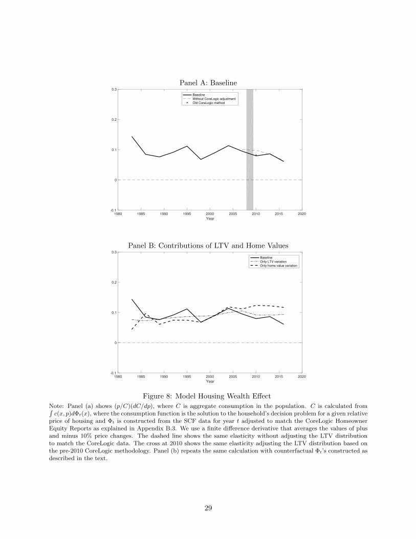
Panel A: Baseline
1980 1985 1990 1995 2000 2005 2010 2015 2020
Year
-0.1
0
0.1
0.2
0.3
Baseline
Without CoreLogic adjustment
Old CoreLogic method
Panel B: Contributions of LTV and Home Values
1980 1985 1990 1995 2000 2005 2010 2015 2020
Year
-0.1
0
0.1
0.2
0.3
Baseline
Only LTV variation
Only home value variation
Figure 8: Model Housing Wealth Effect
Note: Panel (a) shows (p/C)(dC/dp), where C is aggregate consumption in the population. C is calculated from∫c(x, p)dΦt(x), where the consumption function is the solution to the household’s decision problem for a given relative
price of housing and Φt is constructed from the SCF data for year t adjusted to match the CoreLogic HomeownerEquity Reports as explained in Appendix B.3. We use a finite difference derivative that averages the values of plusand minus 10% price changes. The dashed line shows the same elasticity without adjusting the LTV distributionto match the CoreLogic data. The cross at 2010 shows the same elasticity adjusting the LTV distribution based onthe pre-2010 CoreLogic methodology. Panel (b) repeats the same calculation with counterfactual Φt’s constructed asdescribed in the text.
29
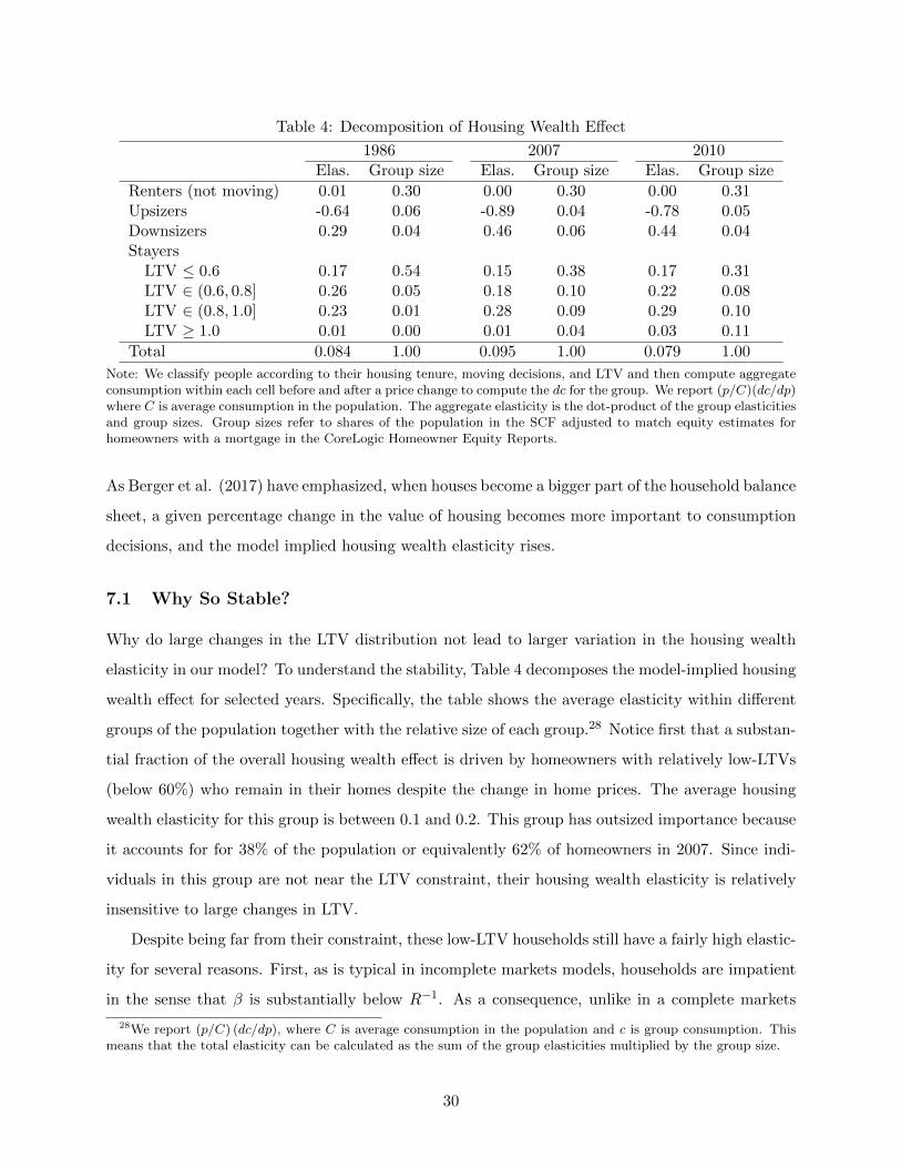
Table 4: Decomposition of Housing Wealth Effect
1986 2007 2010Elas. Group size Elas. Group size Elas. Group size
Renters (not moving) 0.01 0.30 0.00 0.30 0.00 0.31Upsizers -0.64 0.06 -0.89 0.04 -0.78 0.05Downsizers 0.29 0.04 0.46 0.06 0.44 0.04Stayers
LTV ≤ 0.6 0.17 0.54 0.15 0.38 0.17 0.31LTV ∈ (0.6, 0.8] 0.26 0.05 0.18 0.10 0.22 0.08LTV ∈ (0.8, 1.0] 0.23 0.01 0.28 0.09 0.29 0.10LTV ≥ 1.0 0.01 0.00 0.01 0.04 0.03 0.11
Total 0.084 1.00 0.095 1.00 0.079 1.00
Note: We classify people according to their housing tenure, moving decisions, and LTV and then compute aggregateconsumption within each cell before and after a price change to compute the dc for the group. We report (p/C)(dc/dp)where C is average consumption in the population. The aggregate elasticity is the dot-product of the group elasticitiesand group sizes. Group sizes refer to shares of the population in the SCF adjusted to match equity estimates forhomeowners with a mortgage in the CoreLogic Homeowner Equity Reports.
As Berger et al. (2017) have emphasized, when houses become a bigger part of the household balance
sheet, a given percentage change in the value of housing becomes more important to consumption
decisions, and the model implied housing wealth elasticity rises.
7.1 Why So Stable?
Why do large changes in the LTV distribution not lead to larger variation in the housing wealth
elasticity in our model? To understand the stability, Table 4 decomposes the model-implied housing
wealth effect for selected years. Specifically, the table shows the average elasticity within different
groups of the population together with the relative size of each group.28 Notice first that a substan-
tial fraction of the overall housing wealth effect is driven by homeowners with relatively low-LTVs
(below 60%) who remain in their homes despite the change in home prices. The average housing
wealth elasticity for this group is between 0.1 and 0.2. This group has outsized importance because
it accounts for for 38% of the population or equivalently 62% of homeowners in 2007. Since indi-
viduals in this group are not near the LTV constraint, their housing wealth elasticity is relatively
insensitive to large changes in LTV.
Despite being far from their constraint, these low-LTV households still have a fairly high elastic-
ity for several reasons. First, as is typical in incomplete markets models, households are impatient
in the sense that β is substantially below R−1. As a consequence, unlike in a complete markets
28We report (p/C) (dc/dp), where C is average consumption in the population and c is group consumption. Thismeans that the total elasticity can be calculated as the sum of the group elasticities multiplied by the group size.
30
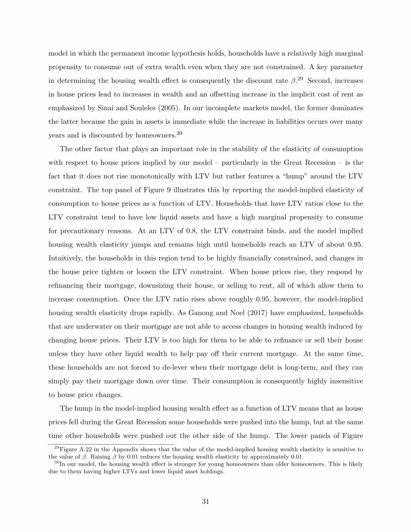
model in which the permanent income hypothesis holds, households have a relatively high marginal
propensity to consume out of extra wealth even when they are not constrained. A key parameter
in determining the housing wealth effect is consequently the discount rate β.29 Second, increases
in house prices lead to increases in wealth and an offsetting increase in the implicit cost of rent as
emphasized by Sinai and Souleles (2005). In our incomplete markets model, the former dominates
the latter because the gain in assets is immediate while the increase in liabilities occurs over many
years and is discounted by homeowners.30
The other factor that plays an important role in the stability of the elasticity of consumption
with respect to house prices implied by our model – particularly in the Great Recession – is the
fact that it does not rise monotonically with LTV but rather features a “hump” around the LTV
constraint. The top panel of Figure 9 illustrates this by reporting the model-implied elasticity of
consumption to house prices as a function of LTV. Households that have LTV ratios close to the
LTV constraint tend to have low liquid assets and have a high marginal propensity to consume
for precautionary reasons. At an LTV of 0.8, the LTV constraint binds, and the model implied
housing wealth elasticity jumps and remains high until households reach an LTV of about 0.95.
Intuitively, the households in this region tend to be highly financially constrained, and changes in
the house price tighten or loosen the LTV constraint. When house prices rise, they respond by
refinancing their mortgage, downsizing their house, or selling to rent, all of which allow them to
increase consumption. Once the LTV ratio rises above roughly 0.95, however, the model-implied
housing wealth elasticity drops rapidly. As Ganong and Noel (2017) have emphasized, households
that are underwater on their mortgage are not able to access changes in housing wealth induced by
changing house prices. Their LTV is too high for them to be able to refinance or sell their house
unless they have other liquid wealth to help pay off their current mortgage. At the same time,
these households are not forced to de-lever when their mortgage debt is long-term, and they can
simply pay their mortgage down over time. Their consumption is consequently highly insensitive
to house price changes.
The hump in the model-implied housing wealth effect as a function of LTV means that as house
prices fell during the Great Recession some households were pushed into the hump, but at the same
time other households were pushed out the other side of the hump. The lower panels of Figure
29Figure A.22 in the Appendix shows that the value of the model-implied housing wealth elasticity is sensitive tothe value of β. Raising β by 0.01 reduces the housing wealth elasticity by approximately 0.01.
30In our model, the housing wealth effect is stronger for young homeowners than older homeowners. This is likelydue to them having higher LTVs and lower liquid asset holdings.
31
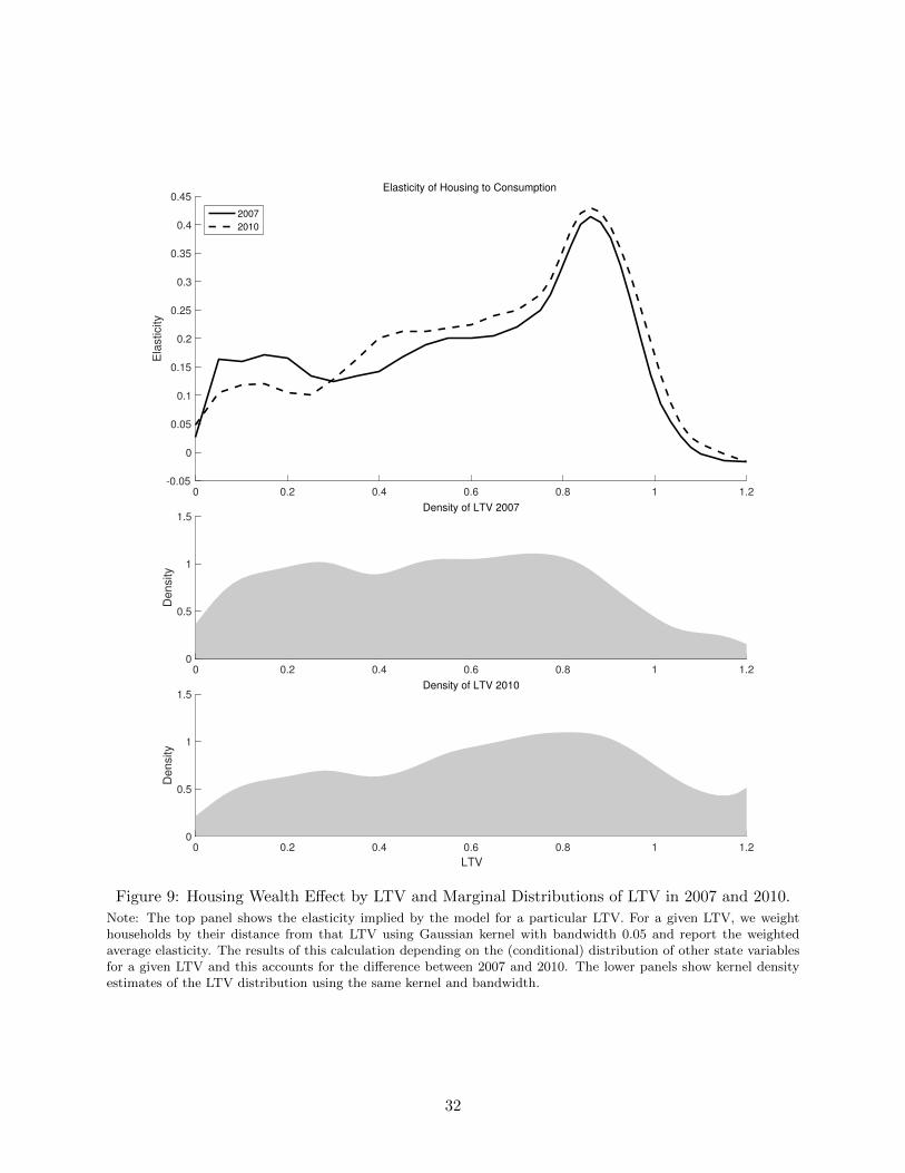
0 0.2 0.4 0.6 0.8 1 1.2-0.05
0
0.05
0.1
0.15
0.2
0.25
0.3
0.35
0.4
0.45
Ela
sticity
Elasticity of Housing to Consumption
2007
2010
0 0.2 0.4 0.6 0.8 1 1.20
0.5
1
1.5
Density
Density of LTV 2007
0 0.2 0.4 0.6 0.8 1 1.2
LTV
0
0.5
1
1.5
Density
Density of LTV 2010
Figure 9: Housing Wealth Effect by LTV and Marginal Distributions of LTV in 2007 and 2010.
Note: The top panel shows the elasticity implied by the model for a particular LTV. For a given LTV, we weighthouseholds by their distance from that LTV using Gaussian kernel with bandwidth 0.05 and report the weightedaverage elasticity. The results of this calculation depending on the (conditional) distribution of other state variablesfor a given LTV and this accounts for the difference between 2007 and 2010. The lower panels show kernel densityestimates of the LTV distribution using the same kernel and bandwidth.
32
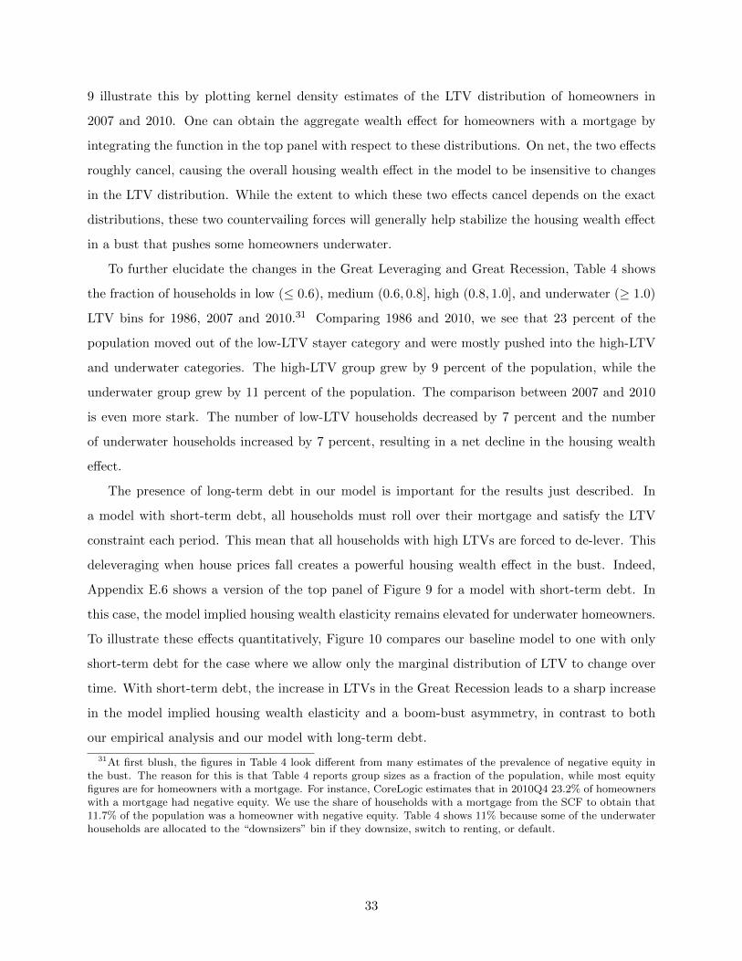
9 illustrate this by plotting kernel density estimates of the LTV distribution of homeowners in
2007 and 2010. One can obtain the aggregate wealth effect for homeowners with a mortgage by
integrating the function in the top panel with respect to these distributions. On net, the two effects
roughly cancel, causing the overall housing wealth effect in the model to be insensitive to changes
in the LTV distribution. While the extent to which these two effects cancel depends on the exact
distributions, these two countervailing forces will generally help stabilize the housing wealth effect
in a bust that pushes some homeowners underwater.
To further elucidate the changes in the Great Leveraging and Great Recession, Table 4 shows
the fraction of households in low (≤ 0.6), medium (0.6, 0.8], high (0.8, 1.0], and underwater (≥ 1.0)
LTV bins for 1986, 2007 and 2010.31 Comparing 1986 and 2010, we see that 23 percent of the
population moved out of the low-LTV stayer category and were mostly pushed into the high-LTV
and underwater categories. The high-LTV group grew by 9 percent of the population, while the
underwater group grew by 11 percent of the population. The comparison between 2007 and 2010
is even more stark. The number of low-LTV households decreased by 7 percent and the number
of underwater households increased by 7 percent, resulting in a net decline in the housing wealth
effect.
The presence of long-term debt in our model is important for the results just described. In
a model with short-term debt, all households must roll over their mortgage and satisfy the LTV
constraint each period. This mean that all households with high LTVs are forced to de-lever. This
deleveraging when house prices fall creates a powerful housing wealth effect in the bust. Indeed,
Appendix E.6 shows a version of the top panel of Figure 9 for a model with short-term debt. In
this case, the model implied housing wealth elasticity remains elevated for underwater homeowners.
To illustrate these effects quantitatively, Figure 10 compares our baseline model to one with only
short-term debt for the case where we allow only the marginal distribution of LTV to change over
time. With short-term debt, the increase in LTVs in the Great Recession leads to a sharp increase
in the model implied housing wealth elasticity and a boom-bust asymmetry, in contrast to both
our empirical analysis and our model with long-term debt.
31At first blush, the figures in Table 4 look different from many estimates of the prevalence of negative equity inthe bust. The reason for this is that Table 4 reports group sizes as a fraction of the population, while most equityfigures are for homeowners with a mortgage. For instance, CoreLogic estimates that in 2010Q4 23.2% of homeownerswith a mortgage had negative equity. We use the share of households with a mortgage from the SCF to obtain that11.7% of the population was a homeowner with negative equity. Table 4 shows 11% because some of the underwaterhouseholds are allocated to the “downsizers” bin if they downsize, switch to renting, or default.
33
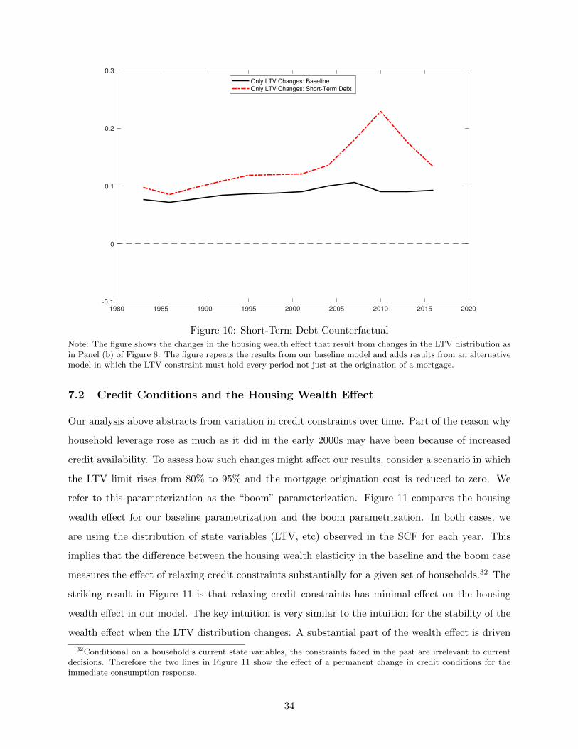
1980 1985 1990 1995 2000 2005 2010 2015 2020-0.1
0
0.1
0.2
0.3
Only LTV Changes: Baseline
Only LTV Changes: Short-Term Debt
Figure 10: Short-Term Debt Counterfactual
Note: The figure shows the changes in the housing wealth effect that result from changes in the LTV distribution asin Panel (b) of Figure 8. The figure repeats the results from our baseline model and adds results from an alternativemodel in which the LTV constraint must hold every period not just at the origination of a mortgage.
7.2 Credit Conditions and the Housing Wealth Effect
Our analysis above abstracts from variation in credit constraints over time. Part of the reason why
household leverage rose as much as it did in the early 2000s may have been because of increased
credit availability. To assess how such changes might affect our results, consider a scenario in which
the LTV limit rises from 80% to 95% and the mortgage origination cost is reduced to zero. We
refer to this parameterization as the “boom” parameterization. Figure 11 compares the housing
wealth effect for our baseline parametrization and the boom parametrization. In both cases, we
are using the distribution of state variables (LTV, etc) observed in the SCF for each year. This
implies that the difference between the housing wealth elasticity in the baseline and the boom case
measures the effect of relaxing credit constraints substantially for a given set of households.32 The
striking result in Figure 11 is that relaxing credit constraints has minimal effect on the housing
wealth effect in our model. The key intuition is very similar to the intuition for the stability of the
wealth effect when the LTV distribution changes: A substantial part of the wealth effect is driven
32Conditional on a household’s current state variables, the constraints faced in the past are irrelevant to currentdecisions. Therefore the two lines in Figure 11 show the effect of a permanent change in credit conditions for theimmediate consumption response.
34
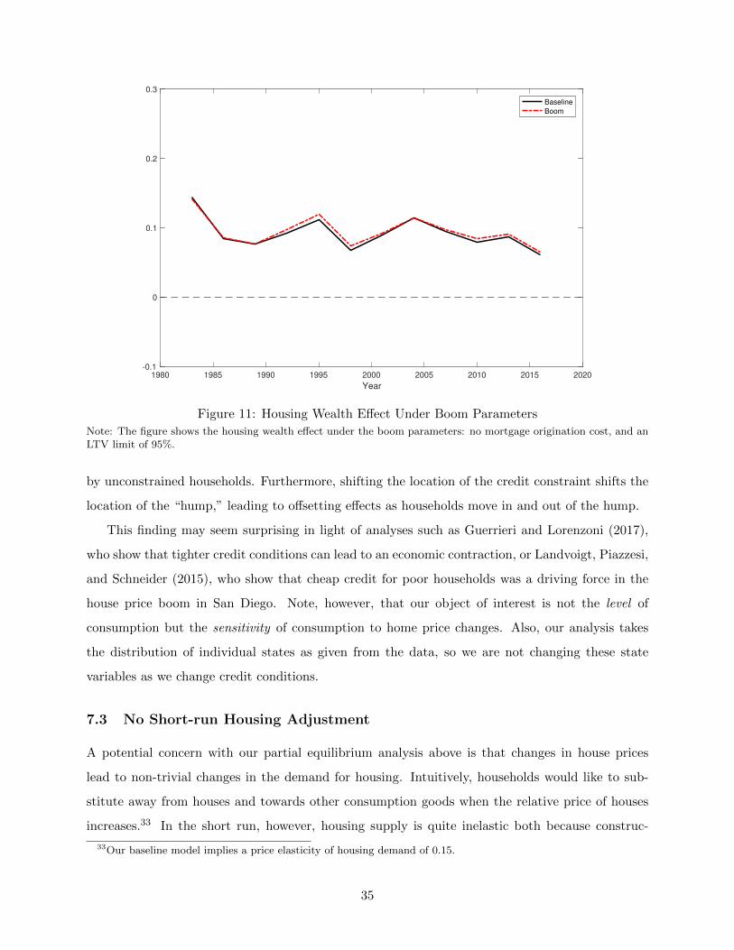
1980 1985 1990 1995 2000 2005 2010 2015 2020
Year
-0.1
0
0.1
0.2
0.3
Baseline
Boom
Figure 11: Housing Wealth Effect Under Boom Parameters
Note: The figure shows the housing wealth effect under the boom parameters: no mortgage origination cost, and anLTV limit of 95%.
by unconstrained households. Furthermore, shifting the location of the credit constraint shifts the
location of the “hump,” leading to offsetting effects as households move in and out of the hump.
This finding may seem surprising in light of analyses such as Guerrieri and Lorenzoni (2017),
who show that tighter credit conditions can lead to an economic contraction, or Landvoigt, Piazzesi,
and Schneider (2015), who show that cheap credit for poor households was a driving force in the
house price boom in San Diego. Note, however, that our object of interest is not the level of
consumption but the sensitivity of consumption to home price changes. Also, our analysis takes
the distribution of individual states as given from the data, so we are not changing these state
variables as we change credit conditions.
7.3 No Short-run Housing Adjustment
A potential concern with our partial equilibrium analysis above is that changes in house prices
lead to non-trivial changes in the demand for housing. Intuitively, households would like to sub-
stitute away from houses and towards other consumption goods when the relative price of houses
increases.33 In the short run, however, housing supply is quite inelastic both because construc-
33Our baseline model implies a price elasticity of housing demand of 0.15.
35

tion of new houses takes time and also because each year’s construction of new houses represents
a small addition of the overall housing stock. This implies that the change in housing demand
implied by our partial equilibrium model is unlikely to be consistent with market clearing in the
housing market.
To address this concern, we consider an alternate experiment in which there is no change in
housing demand in the short run. We compare two cities that both have completely inelastic
housing supply in the short run, but have different long-run housing supply elasticities. These
cities are hit by an aggregate shock that leads house prices to rise by 10% more in the less-elastic
city in the long run. In the short run, house prices are endogenously determined so that housing
demand is unchanged, i.e., the housing market clears with no change in the housing stock. The
short-run equilibrium increase in house prices in the less-elastic city is less than 10%, leaving an
expected capital gain that motivates people in that city to own housing despite its higher relative
price.34
Figure A.28 in the Appendix compares the model-implied housing wealth effect for this alternate
experiment to our baseline model-implied housing wealth elasticity. The demand for housing is
highly sensitive to expected capital gains. Even a small expected capital gain is sufficient to
equilibrate the housing market without any change in quantity of housing. The housing wealth
elasticity in this alternate experiment is virtually identical to our baseline. Hence, while expected
capital gains are a powerful force in affecting the quantity of housing demanded, they have little
effect on the housing wealth elasticity.
7.4 Is the Model Consistent with the Evolution of Household Balance Sheets?
Our theoretical analysis uses the observed distribution of idiosyncratic states instead of the distri-
bution that is generated by the model. Two considerations motivate this approach. First, it allows
us to analyze the consequences of changes in household balance sheets while remaining agnostic
as to the driving forces behind those changes. Second, this approach allows us to match the dis-
tributions of individual states observed in the data as closely as possible. However, a reasonable
question to ask is whether our model is in fact consistent with the observed evolution of household
balance sheets.
To address this question, we simulate the model’s predictions for the evolution of the LTV
34This experiment was motivated in part by the belief shocks of Kaplan, Mitman, and Violante (2017), which raiseexpectations of future housing demand without affecting current preferences. In their general equilibrium model, thebelief shock raises current prices through expectations of future capital gains.
36
distribution in response to the changes in aggregate home prices we observe in the data. We begin
the simulation at each wave of the SCF and ask how the model’s predictions compare to the next
wave of the SCF. For example, we start with the 1983 data and simulate the model using changes
in aggregate home prices for 1983-1986. We then compare the model’s predictions to the SCF data
in 1986. We present the results of this analysis in Figure A.29 in the Appendix. Our baseline
model largely succeeds in fitting the evolution of leverage from the late 1980s until the mid-1990s
and during the Great Recession. The baseline model is less successful during the 1998-2007 period
when the LTV distribution was stable despite a large run-up in house prices.
We can explain the evolution of leverage during the 1998-2007 period if we allow for two addi-
tional plausible features of the housing boom. First, we allow for a relaxation of credit standards
by assuming that the LTV limit rises to 95% and that mortgage origination costs fall to zero for
the years 1998-2007, as in the “boom parameterization” discussed above. Second, we allow for in-
creased optimism of home owners about house prices by assuming one-year expected capital gains
that rise from 0% to 2% from 2004 to 2007. This is motivated by Kaplan, Mitman, and Violante
(2017) who argue that expected capital gains are central to fitting the evolution of house prices
and leverage during the 2000s boom-bust episode.
Figure A.30 shows that if we incorporate these two features, we can fit the stability of the LTV
distribution during the boom despite the large increase in house prices. Intuitively, both features
make households more aggressive in borrowing against their houses, and this explains why house
price appreciation did not mechanically lower LTV’s. Nevertheless, these modifications have a very
limited effect on the housing wealth elasticity. Credit constraints have little effect on the elasticity,
as we discuss in Section 7.2, while allowing for a modest increase in expected capital gains also has
a small effect, increasing the housing wealth effect in 2007 by 16 percent. Appendix E.9 provides
additional details of these simulations. We conclude that modifying our model to fit the evolution of
the states in the boom has little effect on our main conclusions about the housing wealth elasticity.
7.5 Extensions and Robustness
We explore how our results are affected by several other modeling choices in the Appendix. We
show that the housing wealth effect is modestly increasing in mortgage interest rates, which we set
at 3% in our baseline specification (see Figure A.24). At higher interest rates, households are more
likely to downsize their homes and downsizers have large elasticities. This is particularly true of
high-LTV households, who were more common in recent years.
37
Our baseline analysis assumes that rents are proportional to home prices. During the housing
boom of the 2000s, the rent-price ratio fell considerably. Making the polar opposite (and also
unrealistic) assumption that rents remain constant when home prices change yields somewhat
higher housing wealth effects because it leads renters to defer buying a house and spend more on
non-housing consumption. However, this alternate rent assumption does not change the time series
pattern of the wealth effect (see Figure A.25).
A larger cost of selling a home reduces the housing wealth effect in our model. As the transaction
cost increases, homeowners become less willing to realize the capital gain or loss on their houses
and consumption becomes more insulated from price fluctuations. While the moving cost affects
the level of the housing wealth effect, it does not change the time series pattern (see Figure A.27).
Households can default subject to a utility cost in our model, and we set the utility cost at a
level such that the default option is rarely exercised. However, our results are essentially unchanged
if we make default more attractive. This finding is related to the insensitivity of our results to credit
constraints: the housing wealth effect is heavily influenced by low-LTV households.
8 Conclusion
We present new evidence on the housing wealth effect going back to the 1980s. To do so, we develop
a new identification approach that exploits the differential sensitivity of house prices in cities to
regional house price cycles. This allows us to obtain estimates of the housing wealth effect using a
consistent methodology over a long time period. We find no evidence that the elasticity to changes
in house prices was particularly large in the 2000s; if anything, the elasticity was larger prior to
2000. We also find no evidence of a boom-bust asymmetry.
We develop a theoretical framework to interpret our empirical estimates. We show that our
empirical approach yields an estimate of the partial equilibrium effect of house prices on consump-
tion multiplied by a local general equilibrium multiplier that can be approximated by the local
fiscal multiplier. All other general equilibrium effects are soaked up by fixed effects in our regres-
sions. Our empirical approach thus allows us to draw inferences about the effects of house price
fluctuations while remaining agnostic about fundamental shocks that drive house prices. We then
analyze the partial equilibrium multiplier in the context of a “new canonical model” of housing
wealth effects: a standard life-cycle model with borrowing constraints, uninsurable income risk,
illiquid housing, and long-term mortgages.
38
In the model as in the data, there is little response of the housing wealth effect to shifts in the
LTV distribution — even the large run-up in household leverage as house prices fell during the
Great Recession. This arises for two reasons. First, much of the housing wealth elasticity arises
from a substantial housing wealth effect of impatient unconstrained households. Second, while
an increase in the number of highly constrained households during the Great Recession tended to
raise the elasticity, this was offset by an increase in the number of underwater households whose
consumption is very unresponsive to house prices. Both our empirical analysis and model thus
imply that the housing wealth elasticity is a fundamental feature of the economy that was not
driven by special features of the 2000s boom-bust cycle.
39
References
Acemoglu, D., D. Autor, D. Dorn, G. H. Hanson, and B. Price (2016). Import Competition and
the Great U.S. Employment Sag of the 2000s. Journal of Labor Economics 34 (S1), S141–S198.
Adelino, M., A. Schoar, and F. Severino (2015). House Prices, Collateral, and Self-Employment.
Journal of Financial Economics 117 (2), 288–306.
Agarwal, S., G. Amromin, S. Chomsisengphet, T. Landvoigt, T. Piskorski, A. Seru, and V. Yao
(2017). Mortgage Refinancing, Consumer Spending, and Competition: Evidence from the
Home Affordable Refinancing Program.
Aladangady, A. (2017). Housing Wealth and Consumption: Evidence from Geographically-
Linked Microdata. American Economic Review 107 (11), 3415–3446.
Attanasio, O., L. Blow, R. Hamilton, and A. Leicester (2009). Booms and Busts: Consumption,
House Prices, and Expectations. Economica 76 (301), 20–50.
Attanasio, O., A. Leicester, and M. Wakefield (2011). Do House Prices Drive Consumption
Growth? The Coincident Cycles of House Prices and Consumption in the UK. Journal of the
European Economic Association 9 (3), 399–435.
Bailey, M., R. Cao, T. Kuchler, and J. Stroebel (2017). The Economic Effects of Social Networks:
Evidence From the Housing Market.
Berger, D., V. Guerrieri, G. Lorenzoni, and J. Vavra (2017). House Prices and Consumer Spend-
ing.
Bhutta, N. and B. J. Keys (2016). Interest Rates and Equity Extraction During the Housing
Boom. American Economic Review 106 (7), 1742–1774.
Blanchard, O. and L. F. Katz (1992). Regional Evolutions. Brookings Papers on Economic Ac-
tivity 1, 1–75.
Calomiris, C. W., S. D. Longhofer, and W. Miles (2013). The Housing Wealth Effect: The Crucial
Roles of Demographics Wealth Distribution, and Wealth Shares. Critical Finance Review 2,
49–99.
Campbell, J. Y. and J. F. Cocco (2003). Household Risk Management and Optimal Mortgage
Choice. Quarterly Journal of Economics 118 (4), 1449–1494.
40
Campbell, J. Y. and J. F. Cocco (2007). How Do House Prices Affect Consumption? Journal of
Monetary Economics 54 (3), 591–621.
Carroll, C. D., M. Otsuka, and J. Salacalek (2011). How Large Are Housing and Financial Wealth
Effects? A New Approach. Journal of Money, Credit and Banking 43 (1), 55–79.
Case, K. E., R. J. Shiller, and J. M. Quigley (2005). Comparing Wealth Effects: The Stock
Market vs. the Housing Market. Advances in Macroeconomics 5 (1), 1–34.
Case, K. E., R. J. Shiller, and J. M. Quigley (2013). Wealth Effects Revisited, 1975-2012. Critical
Finance Review 2 (1), 101–128.
Chaney, T., D. Sraer, and D. Thesmar (2012). The Collateral Channel: How Real Estate Shocks
Affect Corporate Investment. American Economic Review 102 (6), 2381–2409.
Cloyne, J., K. Huber, E. Ilzetzki, and H. Kleven (2017). The Effect of House Prices on Household
Borrowing: A New Approach.
Cooper, D. (2013). House Price Fluctuations: The Role of Housing Wealth as Borrowing Collat-
eral. The Review of Economics and Statistics 95 (4), 1183–1197.
Davidoff, T. (2016). Supply Constraints Are Not Valid Instrumental Variables for Home Prices
Because They Are Correlated With Many Demand Factors. Critical Finance Review 5 (2),
177–206.
Davis, M. and S. Van Nieuwerburgh (2015). Housing, Finance, and the Macroeconomy. In G. Du-
ranton, J. V. Henderson, and W. C. Strange (Eds.), Handbook of Regional and Urban Eco-
nomics, Volume 5, pp. 753–811. Elsevier.
DeFusco, A. A. (2018). Homeowner Borrowing and Housing Colalteral: New Evidence from
Expiring Price Controls. Journal of Finance 73 (2), 523–573.
Deng, Y., J. M. Quigley, and R. Van Order (2000). Mortgage Terminations, Heterogeneity, and
the Exercise of Mortgage Options. Econometrica 68 (2), 275–307.
Favara, G. and J. Imbs (2015). Credit Supply and the Price of Housing. American Economic
Review 105 (3), 958–992.
Favilukis, J., S. C. Ludvigson, and S. Van Nieuwerburgh (2017). The Macroeconomic Effects of
Housing Wealth, Housing Finance, and Limited Risk-Sharing in General Equilibrium. Journal
of Political Economy 125 (1), 140–223.
41

Flavin, M. and S. Nakagawa (2008). A Model of Housing in the Presence of Adjustment Costs: A
Structural Interpretation of Habit Persistence. American Economic Review 98 (1), 474–495.
Foote, C. L., K. S. Gerardi, and P. S. Willen (2012). Why Did So Many People Make So Many
Ex Post Bad Decisions? The Causes of the Foreclosure Crisis.
Ganong, P. and P. Noel (2017). The Effect of Debt on Default and Consumption: Evidence from
Housing Policy in the Great Recession.
Gilchrist, S. and E. Zakrajsek (2012). Credit Spreads and Business Cycle Fluctuations. American
Economic Review 102 (4), 1692–1720.
Gorea, D. and V. Midrigan (2017). Liquidity Constraints in the U.S. Housing Market.
Guerrieri, L. and M. Iacoviello (2017). Collateral Constraints and Macroeconomic Asymmetries.
Journal of Monetary Economics 90, 28–49.
Guerrieri, V. and G. Lorenzoni (2017). Credit Crises, Precautionary Savings, and the Liquidity
Trap. The Quarterly Journal of Economics 132 (3), 1427–1467.
Guner, N., R. Kaygusuz, and G. Ventura (2014). Income Taxation of U.S. Households: Facts
and Parametric Estimates. Review of Economic Dynamics 17 (4), 559–581.
Guren, A. M., A. Krishnamurthy, and T. McQuade (2018). Mortgage Design in an Equilibrium
Model of the Housing Market.
Guvenen, F. and J. Anthony A. Smith (2014). Inferring Labor Income Risk and Partial Insurance
From Economic Choices. Econometrica 82 (6), 2085–2129.
Guvenen, F., F. Karahan, S. Ozkan, and J. Song (2016). What Do Data on Millions of U.S.
Workers Reveal about Life-Cycle Earnings Dynamics?
Haughwout, A., R. Peach, J. Sporn, and J. Tracy (2013). The Supply Side of the Housing Boom
and Bust of the 2000s. In E. L. Glaeser and T. Sinai (Eds.), Housing and the Financial Crisis,
pp. 69–104. Chicago: University of Chicago Press.
Hurst, E. and F. P. Stafford (2004). Home Is Where the Equity Is: Mortgage Refinancing and
Household Consumption. Journal of Money, Credit, and Banking 36 (6), 985–1014.
Kaplan, G., K. Mitman, and G. L. Violante (2015). Consumption and House Prices in the Great
Recession: Model Meets Evidence.
42
Kaplan, G., K. Mitman, and G. L. Violante (2017). The Housing Boom and Bust: Model Meets
Evidence.
Kaplan, G., G. L. Violante, and G. Kaplan (2016). Non-Durable Consumption and Housing Net
Worth in the Great Recession: Evidence From Easily Accessible Data.
Kaplan, G., G. L. Violante, and J. Weidner (2014). The Wealthy Hand-To-Mouth. Brookings
Papers on Economic Activity (Spring), 77–138.
Kuhn, M., M. Schularick, and U. I. Steins (2017). The Great American Debt Boom, 1949-2013.
Landvoigt, T., M. Piazzesi, and M. Schneider (2015). The Housing Market(s) of San Diego.
American Economic Review 105 (4), 1371–1407.
Li, W. and R. Yao (2007). The Life-Cycle Effects of House Price Changes. Journal of Money,
Credit and Banking 39 (6), 1375–1409.
Liebersohn, J. (2017). Housing Demand, Regional House Prices, and Consumption.
Mallaby, S. (2016). The Man Who Knew: The Life and Times of Alan Greenspan. New York:
Penguin.
Mian, A., K. Rao, and A. Sufi (2013). Household Balance Sheets, Consumption, and the Ecoomic
Slump. Quarterly Journal of Economics 128, 1687–1726.
Mian, A. and A. Sufi (2011). House Prices, Home Equity-Based Borrowing, and the U.S. House-
hold Leverage Crisis. American Economic Review 101 (5), 2132–2156.
Mian, A. and A. Sufi (2014). What Explains the 2007-2009 Drop in Employment? Economet-
rica 82 (6), 2197–2223.
Mian, A. and A. Sufi (2015). House of Debt: How They (and You) Caused the Great Recession,
and How We Can Prevent It from Happening Again. Chicago: University of Chicago Press.
Nakamura, B. E. and J. Steinsson (2014). Fiscal Stimulus in a Monetary Union: Evidence from
US Regions. American Economic Review 104 (3), 753–792.
Nathanson, C. G. and E. Zwick (2017). Arrested Development: Theory and Evidence of Supply-
Side Speculation in the Housing Market.
Palmer, C. (2015). Why Did So Many Subprime Borrowers Default During the Crisis : Loose
Credit or Plummeting Prices ?
43
Piazzesi, M., M. Schneider, and S. Tuzel (2007). Housing, Consumption, and Asset Pricing.
Journal of Financial Economics 83, 531–596.
Roussanov, N., M. Michaux, and H. Chen (2013). Houses as ATMs? Mortgage Refinancing and
Macroeconomic Uncertainty.
Saiz, A. (2010). The Geographic Determinants of Housing Supply Elasticity. Quarterly Journal
of Economics 125 (3), 1253–1296.
Sinai, T. (2013). House Price Moments in Boom-Bust Cycles. In E. L. Glaeser and T. Sinai
(Eds.), Housing and the Financial Crisis, pp. 19–68. Chicago: University of Chicago Press.
Sinai, T. and N. S. Souleles (2005). Owner-Occupied Housing as a Hedge Against Rent Risk.
Quarterly Journal of Economics 120 (2), 763–790.
Wong, A. (2018). Population Aging and the Transmission of Monetary Policy to Consumption.
44
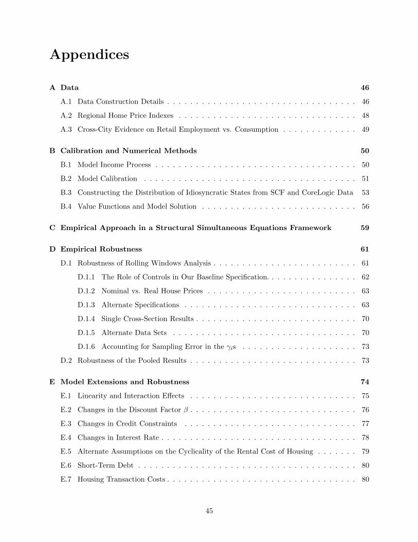
Appendices
A Data 46
A.1 Data Construction Details . . . . . . . . . . . . . . . . . . . . . . . . . . . . . . . . . 46
A.2 Regional Home Price Indexes . . . . . . . . . . . . . . . . . . . . . . . . . . . . . . . 48
A.3 Cross-City Evidence on Retail Employment vs. Consumption . . . . . . . . . . . . . 49
B Calibration and Numerical Methods 50
B.1 Model Income Process . . . . . . . . . . . . . . . . . . . . . . . . . . . . . . . . . . . 50
B.2 Model Calibration . . . . . . . . . . . . . . . . . . . . . . . . . . . . . . . . . . . . . 51
B.3 Constructing the Distribution of Idiosyncratic States from SCF and CoreLogic Data 53
B.4 Value Functions and Model Solution . . . . . . . . . . . . . . . . . . . . . . . . . . . 56
C Empirical Approach in a Structural Simultaneous Equations Framework 59
D Empirical Robustness 61
D.1 Robustness of Rolling Windows Analysis . . . . . . . . . . . . . . . . . . . . . . . . . 61
D.1.1 The Role of Controls in Our Baseline Specification. . . . . . . . . . . . . . . . 62
D.1.2 Nominal vs. Real House Prices . . . . . . . . . . . . . . . . . . . . . . . . . . 63
D.1.3 Alternate Specifications . . . . . . . . . . . . . . . . . . . . . . . . . . . . . . 63
D.1.4 Single Cross-Section Results . . . . . . . . . . . . . . . . . . . . . . . . . . . . 70
D.1.5 Alternate Data Sets . . . . . . . . . . . . . . . . . . . . . . . . . . . . . . . . 70
D.1.6 Accounting for Sampling Error in the γis . . . . . . . . . . . . . . . . . . . . 73
D.2 Robustness of the Pooled Results . . . . . . . . . . . . . . . . . . . . . . . . . . . . . 73
E Model Extensions and Robustness 74
E.1 Linearity and Interaction Effects . . . . . . . . . . . . . . . . . . . . . . . . . . . . . 75
E.2 Changes in the Discount Factor β . . . . . . . . . . . . . . . . . . . . . . . . . . . . . 76
E.3 Changes in Credit Constraints . . . . . . . . . . . . . . . . . . . . . . . . . . . . . . 77
E.4 Changes in Interest Rate . . . . . . . . . . . . . . . . . . . . . . . . . . . . . . . . . . 78
E.5 Alternate Assumptions on the Cyclicality of the Rental Cost of Housing . . . . . . . 79
E.6 Short-Term Debt . . . . . . . . . . . . . . . . . . . . . . . . . . . . . . . . . . . . . . 80
E.7 Housing Transaction Costs . . . . . . . . . . . . . . . . . . . . . . . . . . . . . . . . . 80
45
E.8 No Short Run Housing Adjustment . . . . . . . . . . . . . . . . . . . . . . . . . . . . 82
E.9 Accounting for the Evolution of Household Balance Sheets . . . . . . . . . . . . . . . 84
A Data
A.1 Data Construction Details
Our main data sources are the Quarterly Census of Employment and Wages (QCEW) from 1975 to
2017, the County Business Patterns (CBP) from 1975 to 2016, the 1970-2010 post-Censal county
population estimates, the 2010-2017 inter-Censal county population estimates, and the Freddie
Mac House Price Indices. We also merge in data from a number of other data sources for controls.
Throughout, we use consistent CBSA definitions and assign each CBSA to a census region based
on the majority of its population in the 2000 Census.
The QCEW data provides county-level data for each SIC industry from 1975-2000 and for
each NAICS industry from 1990-2017 and is publicly available on the BLS website. The QCEW
is sometimes missing data due to BLS disclosure requirements, as described by the BLS at:
https://www.bls.gov/osmr/pdf/st040100.pdf. This missing data problem primarily affects smaller
and more narrowly-defined industries in smaller counties where there are few enough employers
within an industry that the BLS’s disclosure criteria are not met. In our baseline analysis, we
only use data for counties within a CBSA that have no missing data for the industry in question
(either retail or manufacturing) over the whole sample. In practice, this means that we drop a few
small outlying counties for a few CBSAs along with the entire Dover, Delaware CBSA. We show
in Appendix D.1.3 that dropping these counties for the entire sample does not affect the results
because they are so small.
The QCEW reports monthly employment and aggregate wages by industry. We take quarterly
averages and use employment for retail or manufacturing employment. We also use the total
wage bill for all employees. We merge in county-level population as estimated annually by the
Census, linearly interpolating to quarters. We then drop counties with missing data at any point
in the sample, aggregate both employment in each industry and population to the CBSA level,
and calculate log changes in employment per capita. The log changes thus begin in 1976 with the
difference between 1976 and 1975 log employment per capita. We create average wages by dividing
total wages by total employment. We then clean the data by removing observations where we
observe an unusually-large jump in employment or employment per capita over a single quarter.
46

We do so because this likely reflects changes such as county realignments or a large employer being
recategorized across industries rather than an actual changes in employment. Appendix D.1.3
shows our results are not sensitive to this data cleaning.
The shift from SIC to NAICS changed the definitions of retail, manufacturing, construction,
and real estate employment. For instance, wholesale employment was included as part of retail
under SIC but separated into its own sector under NAICS. This causes discrete jumps in sectoral
employment. However, for the 1990-2000 period where the BLS provides both SIC and NAICS
data, the two series are almost the same in log changes. We thus splice together the SIC and
NAICS data in Q1 1993. We choose Q1 1993 because this is the first date for which we can splice
together one year and three year log changes. In Appendix D.1.3, we show our results are robust
to splice date
We also use a number of additional variables in constructing controls. We merge in 2-digit
industry shares from the CBP. We use the CBP rather than the QCEW for this because whereas
the QCEW simply omits data when the BLS cannot disclose data, the Census provides employment
ranges for industries that do not satisfy this, which include some 2-digit industries. Because the
CBP data do not provide an overlapping period for SIC and NAICS, we deal with the SIC to
NAICS transition by harmonizing all of the data to consistent 2-digit industry classifications using
an algorithm developed by Acemoglu et al. (2016). We then aggregate to the CBSA level and
create 2-digit industry shares. Because the CBP data are only available through 2016, we assume
that industry shares are constant from 2016 to 2017. Our results are not dependent on this one
year. Since the CBP data are annual, we linearly interpolate to quarters to get a 2-digit industry
share series by quarter. In a robustness check, we also use the annual CBP data rather than the
quarterly QCEW data for the analysis.
We then merge our data set with the Freddie Mac House Price Index. We convert it to a real
index using the GDP deflator downloaded from FRED. In a robustness check, we use FHFA price
indices, which are available for an alternate level of CBSA aggregation. We aggregate everything
to this alternative CBSA definition when using this price index.
We then merge in the Gilchrist and Zakrajsek (2012) excess bond premium. GZ give two
different time series on their website. We use the “ebp oa” measure. This is the excess bond
premium which subtracts a fitted value for “distance to default” from options. We also merge in
the real 30-year mortgage rate, which we create by taking the average 30-year fixed mortgage rate
from FRED and adjusting for inflation using 1-year inflation measured by the BEA’s GDP deflator.
47
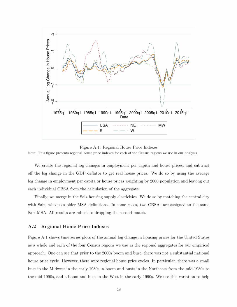
−.2
−.1
0.1
.2A
nn
ua
l L
og
Ch
an
ge
in
Ho
use
Price
s
1975q1 1980q1 1985q1 1990q1 1995q1 2000q1 2005q1 2010q1 2015q1Date
USA NE MW
S W
Figure A.1: Regional House Price Indexes
Note: This figure presents regional house price indexes for each of the Census regions we use in our analysis.
We create the regional log changes in employment per capita and house prices, and subtract
off the log change in the GDP deflator to get real house prices. We do so by using the average
log change in employment per capita or house prices weighting by 2000 population and leaving out
each individual CBSA from the calculation of the aggregate.
Finally, we merge in the Saiz housing supply elasticities. We do so by matching the central city
with Saiz, who uses older MSA definitions. In some cases, two CBSAs are assigned to the same
Saiz MSA. All results are robust to dropping the second match.
A.2 Regional Home Price Indexes
Figure A.1 shows time series plots of the annual log change in housing prices for the United States
as a whole and each of the four Census regions we use as the regional aggregates for our empirical
approach. One can see that prior to the 2000s boom and bust, there was not a substantial national
house price cycle. However, there were regional house price cycles. In particular, there was a small
bust in the Midwest in the early 1980s, a boom and busts in the Northeast from the mid-1980s to
the mid-1990s, and a boom and bust in the West in the early 1990s. We use this variation to help
48
us identify the housing wealth effect prior to 2000.
A.3 Cross-City Evidence on Retail Employment vs. Consumption
In this section, we provide additional evidence on the relationship between retail employment and
consumer expenditures beyond the aggregate evidence presented in the main text by studying
the relationship between city-level consumption and retail employment using data for 17 cities for
which the BLS publishes city-level average consumption per person using data from the Consumer
Expenditure Survey (CEX). Since the aggregated city-level CEX data are available in two-year
averages back to 1986 (e.g., 1986-1987, 1987-1988, and so on), so we construct both the left-hand
side and right-hand side variables as 2-year log differences of the 2-year averaged data.
We estimate:
∆ log Ci,t = ξi + ζt + β∆ log Yi,t + εi,t, (7)
where ∆ log Ci,t is the 2-year log change of 2-year averaged consumption, ∆ log Yi,t is the 2-year log
change of 2-year averaged retail employment, and ξi and ζt are city and time fixed effects respec-
tively. We estimate the equation over the sample period 1986-2014. To construct real consumption,
we deflate consumer expenditures from the CEX by the city-level CPI, which is available from the
BLS for the cities we consider at an annual frequency.
Table A.1 presents the results of this analysis. We estimate this equation both with total
consumption as the dependent variable (columns 1-2) and total consumption excluding imputed
rent (columns 3-4). We first present estimates using OLS. The OLS estimates (column 1 and 3)
show that a 1% increase in retail employment is associated with 0.45-0.55% in total consumption
both including and excluding imputed rent.
However, an important issue in estimating this equation is that the right-hand side variable
(retail employment growth) is measured with substantial error. Hence, the OLS estimate is likely
to be biased downward due to attenuation bias. To account for this, we also present results based
on an IV estimation strategy where we instrument for retail employment using city-level house
price growth. Since the consumption and employment growth rates are for 2-year log changes
in 2-year averages (i.e., the growth rate between say 1997/1996 and 1994/1995) we make use of
3-year log changes in house prices as the instrument (i.e., the house price growth from 1994 to
1997 in this example). It is important to recognize that we are not making any assumption here
about whether variation in the house price index is endogenous or exogenous to business cycle
49
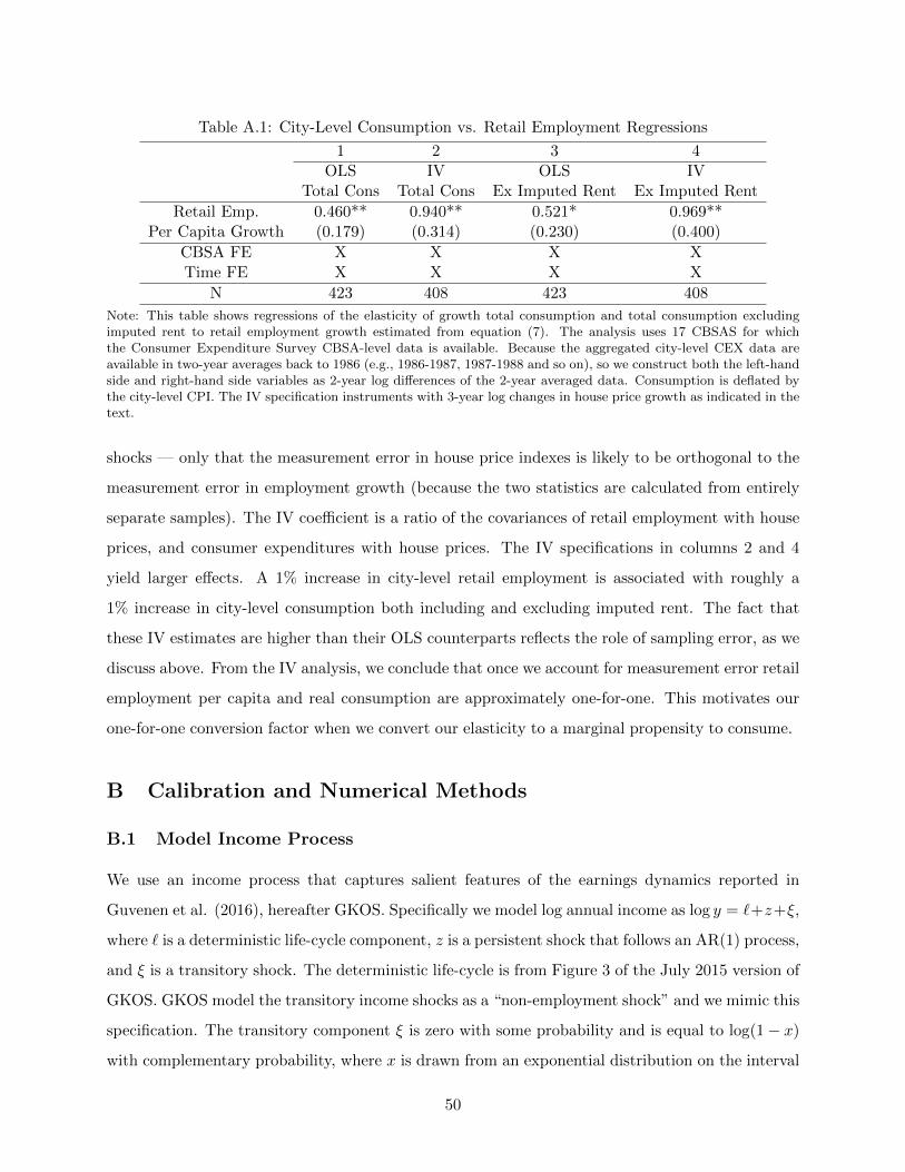
Table A.1: City-Level Consumption vs. Retail Employment Regressions
1 2 3 4OLS IV OLS IV
Total Cons Total Cons Ex Imputed Rent Ex Imputed Rent
Retail Emp. 0.460** 0.940** 0.521* 0.969**Per Capita Growth (0.179) (0.314) (0.230) (0.400)
CBSA FE X X X XTime FE X X X X
N 423 408 423 408
Note: This table shows regressions of the elasticity of growth total consumption and total consumption excludingimputed rent to retail employment growth estimated from equation (7). The analysis uses 17 CBSAS for whichthe Consumer Expenditure Survey CBSA-level data is available. Because the aggregated city-level CEX data areavailable in two-year averages back to 1986 (e.g., 1986-1987, 1987-1988 and so on), so we construct both the left-handside and right-hand side variables as 2-year log differences of the 2-year averaged data. Consumption is deflated bythe city-level CPI. The IV specification instruments with 3-year log changes in house price growth as indicated in thetext.
shocks — only that the measurement error in house price indexes is likely to be orthogonal to the
measurement error in employment growth (because the two statistics are calculated from entirely
separate samples). The IV coefficient is a ratio of the covariances of retail employment with house
prices, and consumer expenditures with house prices. The IV specifications in columns 2 and 4
yield larger effects. A 1% increase in city-level retail employment is associated with roughly a
1% increase in city-level consumption both including and excluding imputed rent. The fact that
these IV estimates are higher than their OLS counterparts reflects the role of sampling error, as we
discuss above. From the IV analysis, we conclude that once we account for measurement error retail
employment per capita and real consumption are approximately one-for-one. This motivates our
one-for-one conversion factor when we convert our elasticity to a marginal propensity to consume.
B Calibration and Numerical Methods
B.1 Model Income Process
We use an income process that captures salient features of the earnings dynamics reported in
Guvenen et al. (2016), hereafter GKOS. Specifically we model log annual income as log y = `+z+ξ,
where ` is a deterministic life-cycle component, z is a persistent shock that follows an AR(1) process,
and ξ is a transitory shock. The deterministic life-cycle is from Figure 3 of the July 2015 version of
GKOS. GKOS model the transitory income shocks as a “non-employment shock” and we mimic this
specification. The transitory component ξ is zero with some probability and is equal to log(1− x)
with complementary probability, where x is drawn from an exponential distribution on the interval
50
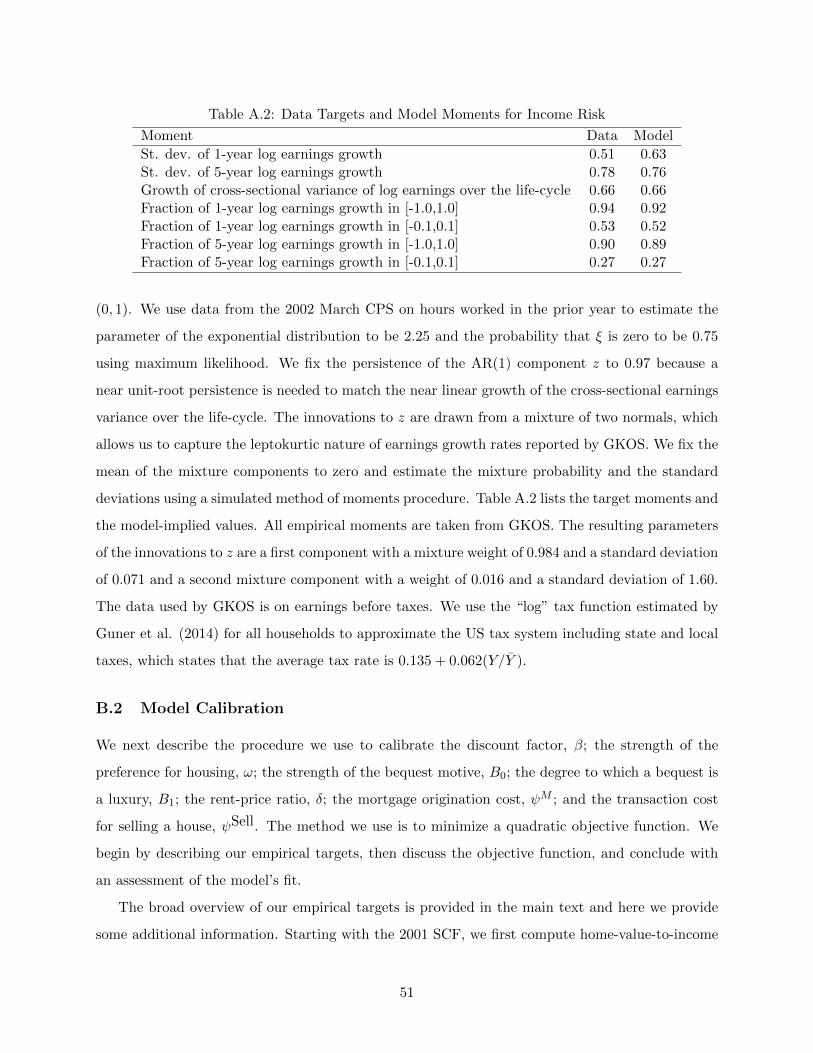
Table A.2: Data Targets and Model Moments for Income Risk
Moment Data Model
St. dev. of 1-year log earnings growth 0.51 0.63St. dev. of 5-year log earnings growth 0.78 0.76Growth of cross-sectional variance of log earnings over the life-cycle 0.66 0.66Fraction of 1-year log earnings growth in [-1.0,1.0] 0.94 0.92Fraction of 1-year log earnings growth in [-0.1,0.1] 0.53 0.52Fraction of 5-year log earnings growth in [-1.0,1.0] 0.90 0.89Fraction of 5-year log earnings growth in [-0.1,0.1] 0.27 0.27
(0, 1). We use data from the 2002 March CPS on hours worked in the prior year to estimate the
parameter of the exponential distribution to be 2.25 and the probability that ξ is zero to be 0.75
using maximum likelihood. We fix the persistence of the AR(1) component z to 0.97 because a
near unit-root persistence is needed to match the near linear growth of the cross-sectional earnings
variance over the life-cycle. The innovations to z are drawn from a mixture of two normals, which
allows us to capture the leptokurtic nature of earnings growth rates reported by GKOS. We fix the
mean of the mixture components to zero and estimate the mixture probability and the standard
deviations using a simulated method of moments procedure. Table A.2 lists the target moments and
the model-implied values. All empirical moments are taken from GKOS. The resulting parameters
of the innovations to z are a first component with a mixture weight of 0.984 and a standard deviation
of 0.071 and a second mixture component with a weight of 0.016 and a standard deviation of 1.60.
The data used by GKOS is on earnings before taxes. We use the “log” tax function estimated by
Guner et al. (2014) for all households to approximate the US tax system including state and local
taxes, which states that the average tax rate is 0.135 + 0.062(Y/Y ).
B.2 Model Calibration
We next describe the procedure we use to calibrate the discount factor, β; the strength of the
preference for housing, ω; the strength of the bequest motive, B0; the degree to which a bequest is
a luxury, B1; the rent-price ratio, δ; the mortgage origination cost, ψM ; and the transaction cost
for selling a house, ψSell. The method we use is to minimize a quadratic objective function. We
begin by describing our empirical targets, then discuss the objective function, and conclude with
an assessment of the model’s fit.
The broad overview of our empirical targets is provided in the main text and here we provide
some additional information. Starting with the 2001 SCF, we first compute home-value-to-income
51
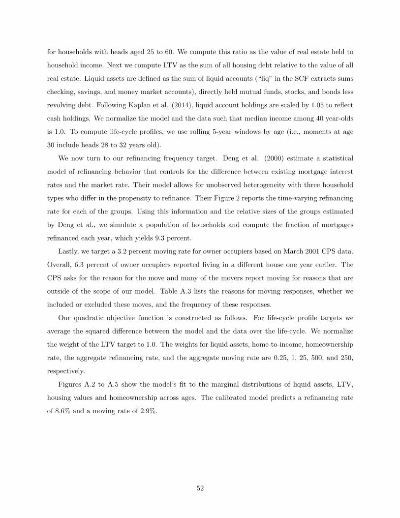
for households with heads aged 25 to 60. We compute this ratio as the value of real estate held to
household income. Next we compute LTV as the sum of all housing debt relative to the value of all
real estate. Liquid assets are defined as the sum of liquid accounts (“liq” in the SCF extracts sums
checking, savings, and money market accounts), directly held mutual funds, stocks, and bonds less
revolving debt. Following Kaplan et al. (2014), liquid account holdings are scaled by 1.05 to reflect
cash holdings. We normalize the model and the data such that median income among 40 year-olds
is 1.0. To compute life-cycle profiles, we use rolling 5-year windows by age (i.e., moments at age
30 include heads 28 to 32 years old).
We now turn to our refinancing frequency target. Deng et al. (2000) estimate a statistical
model of refinancing behavior that controls for the difference between existing mortgage interest
rates and the market rate. Their model allows for unobserved heterogeneity with three household
types who differ in the propensity to refinance. Their Figure 2 reports the time-varying refinancing
rate for each of the groups. Using this information and the relative sizes of the groups estimated
by Deng et al., we simulate a population of households and compute the fraction of mortgages
refinanced each year, which yields 9.3 percent.
Lastly, we target a 3.2 percent moving rate for owner occupiers based on March 2001 CPS data.
Overall, 6.3 percent of owner occupiers reported living in a different house one year earlier. The
CPS asks for the reason for the move and many of the movers report moving for reasons that are
outside of the scope of our model. Table A.3 lists the reasons-for-moving responses, whether we
included or excluded these moves, and the frequency of these responses.
Our quadratic objective function is constructed as follows. For life-cycle profile targets we
average the squared difference between the model and the data over the life-cycle. We normalize
the weight of the LTV target to 1.0. The weights for liquid assets, home-to-income, homeownership
rate, the aggregate refinancing rate, and the aggregate moving rate are 0.25, 1, 25, 500, and 250,
respectively.
Figures A.2 to A.5 show the model’s fit to the marginal distributions of liquid assets, LTV,
housing values and homeownership across ages. The calibrated model predicts a refinancing rate
of 8.6% and a moving rate of 2.9%.
52
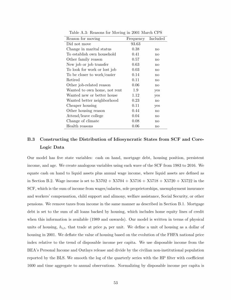
Table A.3: Reasons for Moving in 2001 March CPS
Reason for moving Frequency Included
Did not move 93.63Change in marital status 0.38 noTo establish own household 0.41 noOther family reason 0.57 noNew job or job transfer 0.63 noTo look for work or lost job 0.03 noTo be closer to work/easier 0.14 noRetired 0.11 noOther job-related reason 0.06 noWanted to own home, not rent 1.9 yesWanted new or better house 1.12 yesWanted better neighborhood 0.23 noCheaper housing 0.11 yesOther housing reason 0.44 noAttend/leave college 0.04 noChange of climate 0.08 noHealth reasons 0.06 no
B.3 Constructing the Distribution of Idiosyncratic States from SCF and Core-
Logic Data
Our model has five state variables: cash on hand, mortgage debt, housing position, persistent
income, and age. We create analogous variables using each wave of the SCF from 1983 to 2016. We
equate cash on hand to liquid assets plus annual wage income, where liquid assets are defined as
in Section B.2. Wage income is set to X5702 + X5704 + X5716 + X5718 + X5720 + X5722 in the
SCF, which is the sum of income from wages/salaries, sole proprietorships, unemployment insurance
and workers’ compensation, child support and alimony, welfare assistance, Social Security, or other
pensions. We remove taxes from income in the same manner as described in Section B.1. Mortgage
debt is set to the sum of all loans backed by housing, which includes home equity lines of credit
when this information is available (1989 and onwards). Our model is written in terms of physical
units of housing, hi,t, that trade at price pt per unit. We define a unit of housing as a dollar of
housing in 2001. We deflate the value of housing based on the evolution of the FHFA national price
index relative to the trend of disposable income per capita. We use disposable income from the
BEA’s Personal Income and Outlays release and divide by the civilian non-institutional population
reported by the BLS. We smooth the log of the quarterly series with the HP filter with coefficient
1600 and time aggregate to annual observations. Normalizing by disposable income per capita is
53
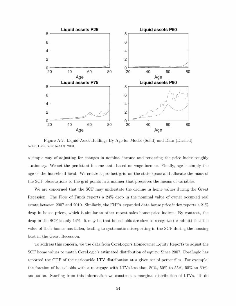
20 40 60 80
Age
0
2
4
6
8Liquid assets P25
20 40 60 80
Age
0
2
4
6
8Liquid assets P50
20 40 60 80
Age
0
2
4
6
8Liquid assets P75
20 40 60 80
Age
0
2
4
6
8Liquid assets P90
Figure A.2: Liquid Asset Holdings By Age for Model (Solid) and Data (Dashed)
Note: Data refer to SCF 2001.
a simple way of adjusting for changes in nominal income and rendering the price index roughly
stationary. We set the persistent income state based on wage income. Finally, age is simply the
age of the household head. We create a product grid on the state space and allocate the mass of
the SCF observations to the grid points in a manner that preserves the means of variables.
We are concerned that the SCF may understate the decline in home values during the Great
Recession. The Flow of Funds reports a 24% drop in the nominal value of owner occupied real
estate between 2007 and 2010. Similarly, the FHFA expanded data house price index reports a 21%
drop in house prices, which is similar to other repeat sales house price indices. By contrast, the
drop in the SCF is only 14%. It may be that households are slow to recognize (or admit) that the
value of their homes has fallen, leading to systematic misreporting in the SCF during the housing
bust in the Great Recession.
To address this concern, we use data from CoreLogic’s Homeowner Equity Reports to adjust the
SCF home values to match CoreLogic’s estimated distribution of equity. Since 2007, CoreLogic has
reported the CDF of the nationwide LTV distribution at a given set of percentiles. For example,
the fraction of households with a mortgage with LTVs less than 50%, 50% to 55%, 55% to 60%,
and so on. Starting from this information we construct a marginal distribution of LTVs. To do
54
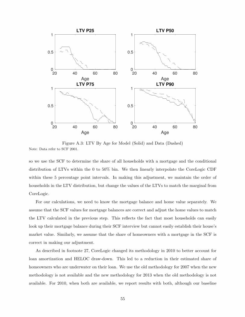
20 40 60 80
Age
0
0.5
1LTV P25
20 40 60 80
Age
0
0.5
1LTV P50
20 40 60 80
Age
0
0.5
1LTV P75
20 40 60 80
Age
0
0.5
1LTV P90
Figure A.3: LTV By Age for Model (Solid) and Data (Dashed)
Note: Data refer to SCF 2001.
so we use the SCF to determine the share of all households with a mortgage and the conditional
distribution of LTVs within the 0 to 50% bin. We then linearly interpolate the CoreLogic CDF
within these 5 percentage point intervals. In making this adjustment, we maintain the order of
households in the LTV distribution, but change the values of the LTVs to match the marginal from
CoreLogic.
For our calculations, we need to know the mortgage balance and home value separately. We
assume that the SCF values for mortgage balances are correct and adjust the home values to match
the LTV calculated in the previous step. This reflects the fact that most households can easily
look up their mortgage balance during their SCF interview but cannot easily establish their house’s
market value. Similarly, we assume that the share of homeowners with a mortgage in the SCF is
correct in making our adjustment.
As described in footnote 27, CoreLogic changed its methodology in 2010 to better account for
loan amortization and HELOC draw-down. This led to a reduction in their estimated share of
homeowners who are underwater on their loan. We use the old methodology for 2007 when the new
methodology is not available and the new methodology for 2013 when the old methodology is not
available. For 2010, when both are available, we report results with both, although our baseline
55
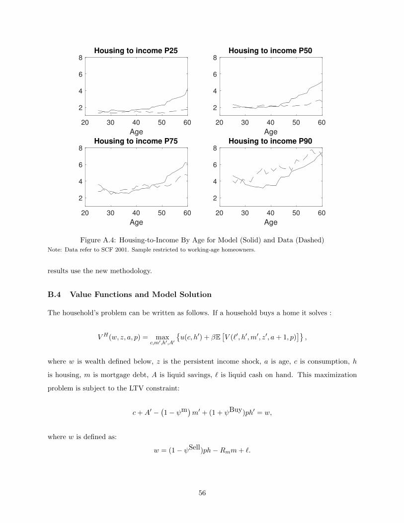
20 30 40 50 60
Age
2
4
6
8Housing to income P25
20 30 40 50 60
Age
2
4
6
8Housing to income P50
20 30 40 50 60
Age
2
4
6
8Housing to income P75
20 30 40 50 60
Age
2
4
6
8Housing to income P90
Figure A.4: Housing-to-Income By Age for Model (Solid) and Data (Dashed)
Note: Data refer to SCF 2001. Sample restricted to working-age homeowners.
results use the new methodology.
B.4 Value Functions and Model Solution
The household’s problem can be written as follows. If a household buys a home it solves :
V H(w, z, a, p) = maxc,m′,h′,A′
u(c, h′) + βE
[V (`′, h′,m′, z′, a+ 1, p)
],
where w is wealth defined below, z is the persistent income shock, a is age, c is consumption, h
is housing, m is mortgage debt, A is liquid savings, ` is liquid cash on hand. This maximization
problem is subject to the LTV constraint:
c+A′ −(1− ψm)m′ + (1 + ψBuy)ph′ = w,
where w is defined as:
w = (1− ψSell)ph−Rmm+ `.
56
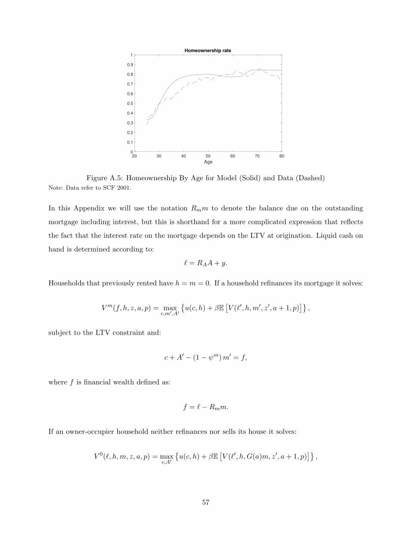
20 30 40 50 60 70 80
Age
0
0.1
0.2
0.3
0.4
0.5
0.6
0.7
0.8
0.9
1Homeownership rate
Figure A.5: Homeownership By Age for Model (Solid) and Data (Dashed)
Note: Data refer to SCF 2001.
In this Appendix we will use the notation Rmm to denote the balance due on the outstanding
mortgage including interest, but this is shorthand for a more complicated expression that reflects
the fact that the interest rate on the mortgage depends on the LTV at origination. Liquid cash on
hand is determined according to:
` = RAA+ y.
Households that previously rented have h = m = 0. If a household refinances its mortgage it solves:
V m(f, h, z, a, p) = maxc,m′,A′
u(c, h) + βE
[V (`′, h,m′, z′, a+ 1, p)
],
subject to the LTV constraint and:
c+A′ − (1− ψm)m′ = f,
where f is financial wealth defined as:
f = `−Rmm.
If an owner-occupier household neither refinances nor sells its house it solves:
V 0(`, h,m, z, a, p) = maxc,A′
u(c, h) + βE
[V (`′, h,G(a)m, z′, a+ 1, p)
],
57
subject to:
c+A′ −m′ = `−Rmm.
A renter solves:
V R(w, z, a, p) = maxc,h′,A′
u(c, h′) + βE
[V (`′, 0, 0, z′, a+ 1, p)
].
Entering the next period, the household has a discrete choice over the adjustment costs:
V (`, h,m, z, a) = maxV H
(((1− ψSell
H )ph−Rmm+ `, z, a, p),
V m (`−Rmm,h, z, a, p) ,
V 0(`, h,m, z, a, p),
V R(
(1− ψsellH − δ)ph+ `−Rmm, z, a, p
),
V D (z, a, p),
with V m and V 0 unavailable to households that previously rented. V D(z, a, p) = V R(ε, z, a, p)− φ
is an option to default on the mortgage, which leaves the household as a renter with a small liquid
asset position ε and incurs a utility cost φ. Defaults play very little role in our analysis (we set
φ = 4 and homeowners are loathe to default), but it is useful to allow this option for homeowners
without alternatives.
We solve the household’s problem using value function iteration. In solving the model we place
a grid on LTV as opposed to mortgage debt. We also specify grids for wealth, financial wealth,
liquid wealth, and income. We allow the household to make continuous choices of consumption,
liquid savings, and mortgage debt, but we restrict housing to discrete values. The output of each
iteration of our Bellman equation is the value on the grid points for (`, h,m, z, a). The most obvious
way of solving this problem is to solve for the optimal actions for each of the discrete adjustment
options for each combination (`, h,m, z, a). A more efficient approach makes use of the fact that, for
example, all households with a certain level of wealth who buy a house will make the same choice
so we can solve the problem on the more compact space of (W, z, a) and then interpolate the value
onto (`, h,m, z, a). This works well for the value functions but there is a small complication for the
decision rules because the housing quantity choice is discrete and so we cannot easily interpolate
the decision rules onto (`, h,m, z, a). To find the decision rules, we cannot avoid solving the problem
58
for the specific combinations of (`, h,m, z, a), but we only need to do this for the households who
choose to buy a new house or rent a house and are therefore making a choice over h′. For households
who refinance, h′ is fixed so there is no problem interpolating the decision rules.
C Empirical Approach in a Structural Simultaneous Equations
Framework
This Appendix explains our identification strategy using a simple simultaneous equations economet-
ric framework. It derives the equation we use to create our instrument structurally and formalizes
our identification assumption.
Consider the following empirical model for the determination of retail employment and house
prices:
∆yi,r,t = ψi + ξr,t + β∆pi,r,t + αiEr,t + εi,r,t, (8)
∆pi,r,t = ϕi + ζr,t + δ∆yi,r,t + γiVr,t + νi,r,t. (9)
We allow for CBSA fixed effects (ψi and ϕi) and region-time fixed effects (ξr,t and ζr,t). Vr,t and
νi,r,t denote regional and idiosyncratic shocks that affect house prices, respectively. Er,t and εi,r,t
denote regional and idiosyncratic shocks that affect retail employment, respectively. These shocks
should be viewed as vectors of more primitive shocks and may be correlated with each other (e.g.,
Vr,t and Er,t may be correlated). Measurement error in retail employment and house prices would
show up in this model as a correlation between νi,r,t and εi,r,t. The model allows for heterogeneity
in sensitivity to regional shocks across CBSAs within region (the i subscripts on αi and γi). This
feature will play an important role. Equation (8) is the analog of equation (1) in the main text and
the coefficient of interest is β, the causal effect of house prices on retail employment measured as
an elasticity.35
Equations (8) and (9) form a system of simultaneous equations. Changes in local house prices
affect local retail employment through the β∆pi,r,t term in equation (8). However, changes in local
employment also affect local house prices through the δ∆yi,r,t term in equation (9). Since causation
between local employment and house prices runs both ways, estimating equation (8) by OLS will
35The empirical model also allows for heterogeneity in the sensitivity to idiosyncratic shocks. This feature iscaptured through heterogeneity in the variances of εi,r,t and νi,r,t in the cross-section. Because this is less importantfor our empirical approach, the notation in equation (8) and (9) is not as explicit about this heterogeneity in sensitivity.
59
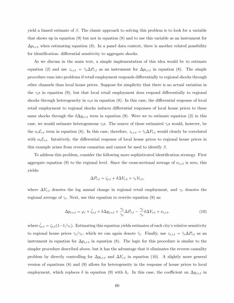
yield a biased estimate of β. The classic approach to solving this problem is to look for a variable
that shows up in equation (9) but not in equation (8) and to use this variable as an instrument for
∆pi,r,t when estimating equation (8). In a panel data context, there is another related possibility
for identification: differential sensitivity to aggregate shocks.
As we discuss in the main text, a simple implementation of this idea would be to estimate
equation (2) and use zi,r,t = γi∆Pr,t as an instrument for ∆pi,r,t in equation (8). The simple
procedure runs into problems if retail employment responds differentially to regional shocks through
other channels than local house prices. Suppose for simplicity that there is no actual variation in
the γis in equation (9), but that local retail employment does respond differentially to regional
shocks through heterogeneity in αis in equation (8). In this case, the differential response of local
retail employment to regional shocks induces differential responses of local house prices to these
same shocks through the δ∆yi,r,t term in equation (9). Were we to estimate equation (2) in this
case, we would estimate heterogeneous γis. The source of these estimated γis would, however, be
the αiEr,t term in equation (8). In this case, therefore, zi,r,t = γi∆Pr,t would clearly be correlated
with αiEr,t. Intuitively, the differential response of local house prices to regional house prices in
this example arises from reverse causation and cannot be used to identify β.
To address this problem, consider the following more sophisticated identification strategy. First
aggregate equation (9) to the regional level. Since the cross-sectional average of νi,r,t is zero, this
yields:
∆Pr,t = ζr,t + δ∆Yr,t + γrVr,t,
where ∆Yr,t denotes the log annual change in regional retail employment, and γr denotes the
regional average of γi. Next, use this equation to rewrite equation (9) as:
∆pi,r,t = ϕi + ζr,t + δ∆yi,r,t +γiγr
∆Pr,t −γiγrδ∆Yr,t + νi,r,t. (10)
where ζr,t = ζr,t(1−1/γr). Estimating this equation yields estimates of each city’s relative sensitivity
to regional house prices γi/γr, which we can again denote γi. Finally, use zi,r,t = γi∆Pr,t as an
instrument in equation for ∆pi,r,t in equation (8). The logic for this procedure is similar to the
simpler procedure described above, but it has the advantage that it eliminates the reverse causality
problem by directly controlling for ∆yi,r,t and ∆Yr,t in equation (10). A slightly more general
version of equations (8) and (9) allows for heterogeneity in the response of house prices to local
employment, which replaces δ in equation (9) with δi. In this case, the coefficient on ∆yi,r,t in
60
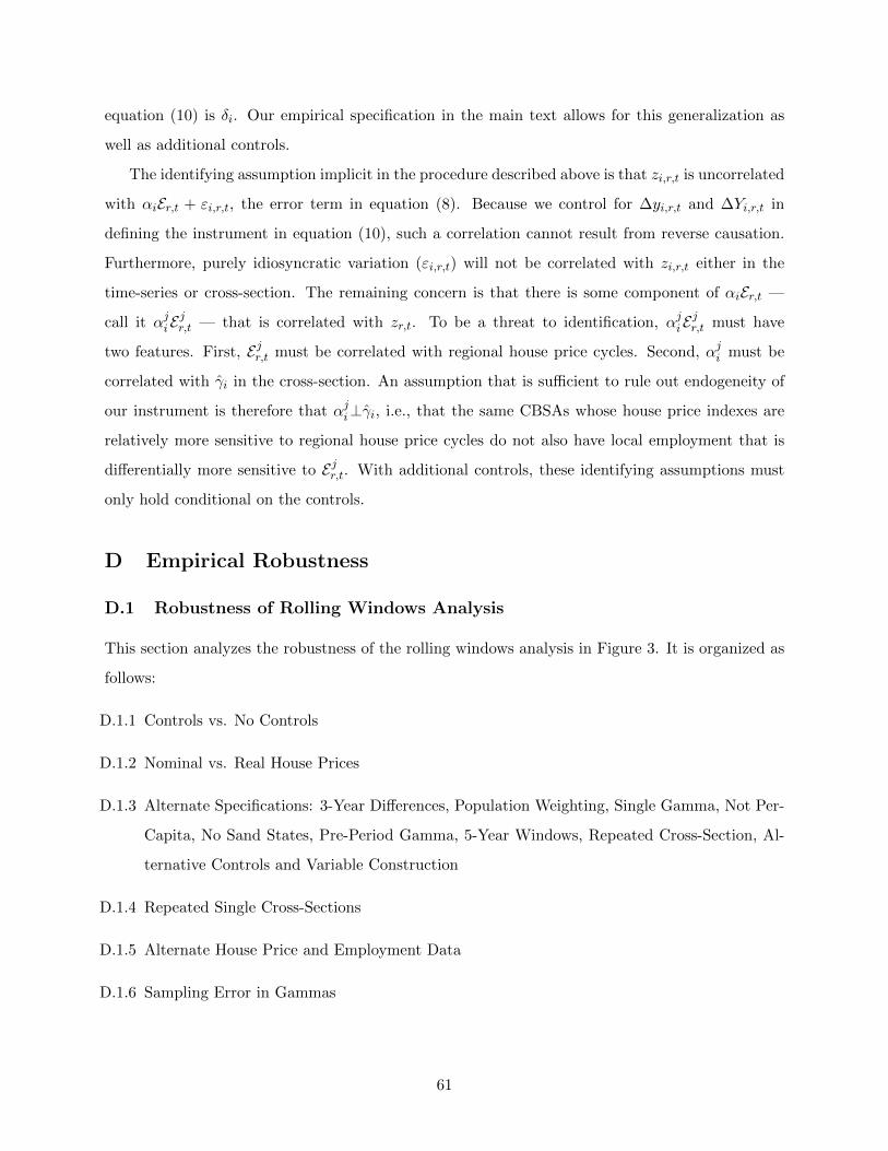
equation (10) is δi. Our empirical specification in the main text allows for this generalization as
well as additional controls.
The identifying assumption implicit in the procedure described above is that zi,r,t is uncorrelated
with αiEr,t + εi,r,t, the error term in equation (8). Because we control for ∆yi,r,t and ∆Yi,r,t in
defining the instrument in equation (10), such a correlation cannot result from reverse causation.
Furthermore, purely idiosyncratic variation (εi,r,t) will not be correlated with zi,r,t either in the
time-series or cross-section. The remaining concern is that there is some component of αiEr,t —
call it αjiEjr,t — that is correlated with zr,t. To be a threat to identification, αjiE
jr,t must have
two features. First, Ejr,t must be correlated with regional house price cycles. Second, αji must be
correlated with γi in the cross-section. An assumption that is sufficient to rule out endogeneity of
our instrument is therefore that αji⊥γi, i.e., that the same CBSAs whose house price indexes are
relatively more sensitive to regional house price cycles do not also have local employment that is
differentially more sensitive to Ejr,t. With additional controls, these identifying assumptions must
only hold conditional on the controls.
D Empirical Robustness
D.1 Robustness of Rolling Windows Analysis
This section analyzes the robustness of the rolling windows analysis in Figure 3. It is organized as
follows:
D.1.1 Controls vs. No Controls
D.1.2 Nominal vs. Real House Prices
D.1.3 Alternate Specifications: 3-Year Differences, Population Weighting, Single Gamma, Not Per-
Capita, No Sand States, Pre-Period Gamma, 5-Year Windows, Repeated Cross-Section, Al-
ternative Controls and Variable Construction
D.1.4 Repeated Single Cross-Sections
D.1.5 Alternate House Price and Employment Data
D.1.6 Sampling Error in Gammas
61
0.1
.2.3
.4.5
IV E
lasticity o
f R
eta
il E
mp to H
ouse P
rices
1990q1 1995q1 2000q1 2005q1 2010q1Midpoint of 10 Year Window
No Controls Controls
Figure A.6: Elasticity of Retail Employment Per Capita to House Prices: No Controls vs. Controls
Note: The figure plots the elasticity of retail employment per capita to real house prices at the CBSA level forrolling 10-year sample periods as in Figure 3 in red (dashed) and a version without the controls used in our baselinespecification in blue. Each point indicates the elasticity for a 10-year sample period with its midpoint in the quarterindicated on the horizontal axis. We use an instrumental variables estimator that is described in Section 3. Confidenceintervals are similar to Figure 3 and are not shown so that the comparison between the two specifications is clearer.
D.1.1 The Role of Controls in Our Baseline Specification.
In our baseline specification, we include a number of controls in the estimation of equations (1) and
(3). These include controls for differential city-level exposure to regional retail employment, real
30-year mortgage rates, and Gilchirst and Zakrajek’s (2012) measure of bond risk premia, controls
for 2-digit industry shares with time-specific coefficients, and, in equation (3), the log change in
average wages with city-specific coefficients.
To evaluate the role of these controls in our results, Figure A.6 shows the point estimates for the
case with controls and the case with no controls (the standard errors do not change significantly).
One can see that the effect is about 25% bigger without controls in the 10-year windows with their
midpoints after 1996. For the 10-year windows with their midpoints prior to 1996, the controls
do much more to reduce the estimated elasticity. Without controls, the pooled estimate of the
elasticity post-1990 is 0.088 rather than 0.071.
Which controls matter the most? In unreported results, we find that the industry shares have
the largest effect, although the control for city-level exposure to regional retail employment does
also explain a significant portion of the gap between the controls and no controls specifications in
the 2000s.
62
−.1
0.1
.2IV
Ela
sticity o
f R
eta
il E
mp to H
ouse P
rices
1990q1 1995q1 2000q1 2005q1 2010q1Midpoint of 10 Year Window
Nominal HPI Real HPI
Figure A.7: Elasticity of Retail Employment Per Capita to House Prices: Real vs. Nominal
Note: The figure plots the elasticity of retail employment per capita to real house prices at the CBSA level for rolling10-year sample periods as in Figure 3 in red (dashed) and a version using nominal house prices in blue. Each pointindicates the elasticity for a 10-year sample period with its midpoint in the quarter indicated on the horizontal axis.We use an instrumental variables estimator that is described in Section 3. Confidence intervals are similar to Figure3 and are not shown so that the comparison between the two specifications is clearer.
D.1.2 Nominal vs. Real House Prices
In our main analysis, we convert to real house prices using the GDP deflator. Figure A.7 compares
our main estimates to an identical specification that uses nominal house prices instead. The results
are broadly similar, although the nominal HPI gives slightly larger results for 10-year windows with
their midpoint in the late-1990s and early 2000s while the real HPI gives slightly larger results for
10-year windows with their midpoint in the late 2000s and early 2010s. On net, the post-1990
pooled elasticity of 0.071 is slightly higher for real house prices than the equivalent elasticity of
0.062 for nominal house prices. These results show that our findings are not due to using a real
house price index.
D.1.3 Alternate Specifications
In this section, we evaluate several alternate specifications. All of the specifications yield a pattern
of declining housing wealth elasticities in rolling windows since 1995. The most important form of
variation across specifications is that several specifications yield lower estimates of the elasticities
in 10-year windows with their midpoint in the early 1990s than in our baseline analysis (though
with large standard errors). This is why we do not put too much emphasis on the 1980s and early
63
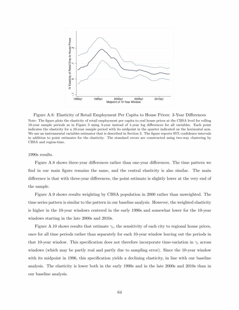
−.1
0.1
.2IV
Ela
sticity o
f R
eta
il E
mp to H
ouse P
rices
1990q1 1995q1 2000q1 2005q1 2010q1Midpoint of 10 Year Window
Figure A.8: Elasticity of Retail Employment Per Capita to House Prices: 3-Year Differences
Note: The figure plots the elasticity of retail employment per capita to real house prices at the CBSA level for rolling10-year sample periods as in Figure 3 using 3-year instead of 1-year log differences for all variables. Each pointindicates the elasticity for a 10-year sample period with its midpoint in the quarter indicated on the horizontal axis.We use an instrumental variables estimator that is described in Section 3. The figure reports 95% confidence intervalsin addition to point estimates for the elasticity. The standard errors are constructed using two-way clustering byCBSA and region-time.
1990s results.
Figure A.8 shows three-year differences rather than one-year differences. The time pattern we
find in our main figure remains the same, and the central elasticity is also similar. The main
difference is that with three-year differences, the point estimate is slightly lower at the very end of
the sample.
Figure A.9 shows results weighting by CBSA population in 2000 rather than unweighted. The
time series pattern is similar to the pattern in our baseline analysis. However, the weighted elasticity
is higher in the 10-year windows centered in the early 1990s and somewhat lower for the 10-year
windows starting in the late 2000s and 2010s.
Figure A.10 shows results that estimate γi, the sensitivity of each city to regional house prices,
once for all time periods rather than separately for each 10-year window leaving out the periods in
that 10-year window. This specification does not therefore incorporate time-variation in γi across
windows (which may be partly real and partly due to sampling error). Since the 10-year window
with its midpoint in 1996, this specification yields a declining elasticity, in line with our baseline
analysis. The elasticity is lower both in the early 1990s and in the late 2000s and 2010s than in
our baseline analysis.
64
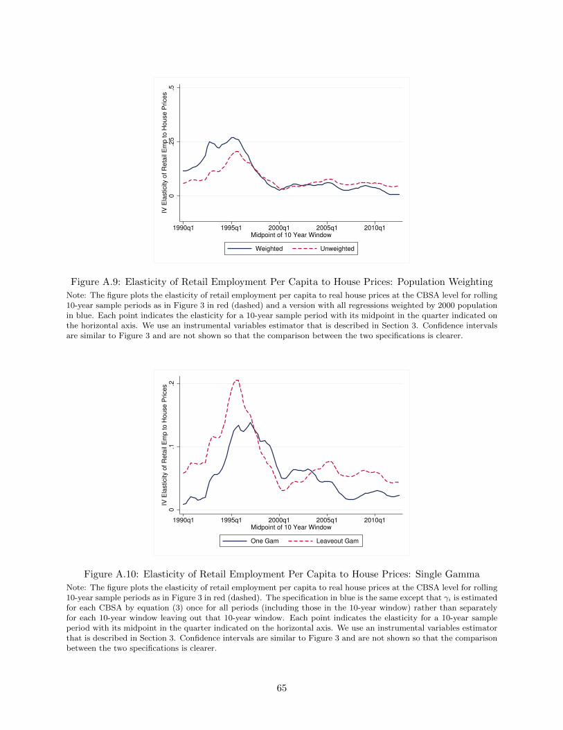
0.2
5.5
IV E
lasticity o
f R
eta
il E
mp to H
ouse P
rices
1990q1 1995q1 2000q1 2005q1 2010q1Midpoint of 10 Year Window
Weighted Unweighted
Figure A.9: Elasticity of Retail Employment Per Capita to House Prices: Population Weighting
Note: The figure plots the elasticity of retail employment per capita to real house prices at the CBSA level for rolling10-year sample periods as in Figure 3 in red (dashed) and a version with all regressions weighted by 2000 populationin blue. Each point indicates the elasticity for a 10-year sample period with its midpoint in the quarter indicated onthe horizontal axis. We use an instrumental variables estimator that is described in Section 3. Confidence intervalsare similar to Figure 3 and are not shown so that the comparison between the two specifications is clearer.
0.1
.2IV
Ela
sticity o
f R
eta
il E
mp to H
ouse P
rices
1990q1 1995q1 2000q1 2005q1 2010q1Midpoint of 10 Year Window
One Gam Leaveout Gam
Figure A.10: Elasticity of Retail Employment Per Capita to House Prices: Single Gamma
Note: The figure plots the elasticity of retail employment per capita to real house prices at the CBSA level for rolling10-year sample periods as in Figure 3 in red (dashed). The specification in blue is the same except that γi is estimatedfor each CBSA by equation (3) once for all periods (including those in the 10-year window) rather than separatelyfor each 10-year window leaving out that 10-year window. Each point indicates the elasticity for a 10-year sampleperiod with its midpoint in the quarter indicated on the horizontal axis. We use an instrumental variables estimatorthat is described in Section 3. Confidence intervals are similar to Figure 3 and are not shown so that the comparisonbetween the two specifications is clearer.
65
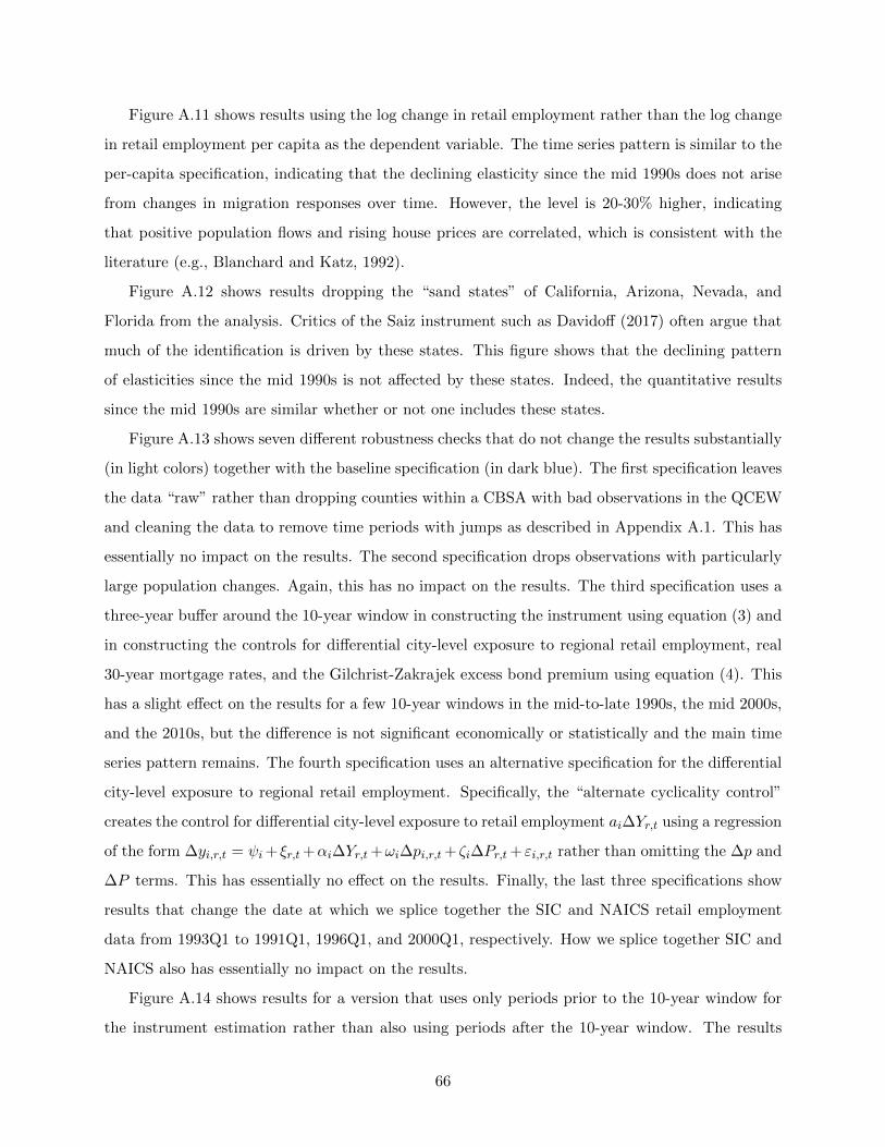
Figure A.11 shows results using the log change in retail employment rather than the log change
in retail employment per capita as the dependent variable. The time series pattern is similar to the
per-capita specification, indicating that the declining elasticity since the mid 1990s does not arise
from changes in migration responses over time. However, the level is 20-30% higher, indicating
that positive population flows and rising house prices are correlated, which is consistent with the
literature (e.g., Blanchard and Katz, 1992).
Figure A.12 shows results dropping the “sand states” of California, Arizona, Nevada, and
Florida from the analysis. Critics of the Saiz instrument such as Davidoff (2017) often argue that
much of the identification is driven by these states. This figure shows that the declining pattern
of elasticities since the mid 1990s is not affected by these states. Indeed, the quantitative results
since the mid 1990s are similar whether or not one includes these states.
Figure A.13 shows seven different robustness checks that do not change the results substantially
(in light colors) together with the baseline specification (in dark blue). The first specification leaves
the data “raw” rather than dropping counties within a CBSA with bad observations in the QCEW
and cleaning the data to remove time periods with jumps as described in Appendix A.1. This has
essentially no impact on the results. The second specification drops observations with particularly
large population changes. Again, this has no impact on the results. The third specification uses a
three-year buffer around the 10-year window in constructing the instrument using equation (3) and
in constructing the controls for differential city-level exposure to regional retail employment, real
30-year mortgage rates, and the Gilchrist-Zakrajek excess bond premium using equation (4). This
has a slight effect on the results for a few 10-year windows in the mid-to-late 1990s, the mid 2000s,
and the 2010s, but the difference is not significant economically or statistically and the main time
series pattern remains. The fourth specification uses an alternative specification for the differential
city-level exposure to regional retail employment. Specifically, the “alternate cyclicality control”
creates the control for differential city-level exposure to retail employment ai∆Yr,t using a regression
of the form ∆yi,r,t = ψi+ ξr,t+αi∆Yr,t+ωi∆pi,r,t+ ζi∆Pr,t+εi,r,t rather than omitting the ∆p and
∆P terms. This has essentially no effect on the results. Finally, the last three specifications show
results that change the date at which we splice together the SIC and NAICS retail employment
data from 1993Q1 to 1991Q1, 1996Q1, and 2000Q1, respectively. How we splice together SIC and
NAICS also has essentially no impact on the results.
Figure A.14 shows results for a version that uses only periods prior to the 10-year window for
the instrument estimation rather than also using periods after the 10-year window. The results
66
−.1
0.1
.2.3
.4IV
Ela
sticity o
f R
eta
il E
mp to H
ouse P
rices
1990q1 1995q1 2000q1 2005q1 2010q1Midpoint of 10 Year Window
Figure A.11: Elasticity of Retail Employment (Not Per Capita) to House Prices
Note: The figure plots the elasticity of retail employment (not per capita) to real house prices at the CBSA level forrolling 10-year sample periods as in Figure 3 except with retail employment rather than retail employment per capitaas the dependent variable. Each point indicates the elasticity for a 10-year sample period with its midpoint in thequarter indicated on the horizontal axis. We use an instrumental variables estimator that is described in Section 3.The figure reports 95% confidence intervals in addition to point estimates for the elasticity. The standard errors areconstructed using two-way clustering by CBSA and region-time.
0.2
5.5
IV E
lasticity o
f R
eta
il E
mp to H
ouse P
rices
1990q1 1995q1 2000q1 2005q1 2010q1Midpoint of 10 Year Window
No Sand States Full Sample
Figure A.12: Elasticity of Retail Employment Per Capita to House Prices: No Sand States
Note: The figure plots the elasticity of retail employment per capita to real house prices at the CBSA level for rolling10-year sample periods as in Figure 3 in red (dashed) and a version dropping the “sand states” of California, Nevada,Arizona, and Florida in blue. Each point indicates the elasticity for a 10-year sample period with its midpoint in thequarter indicated on the horizontal axis. We use an instrumental variables estimator that is described in Section 3.Confidence intervals are similar to Figure 3 and are not shown so that the comparison between the two specificationsis clearer.
67
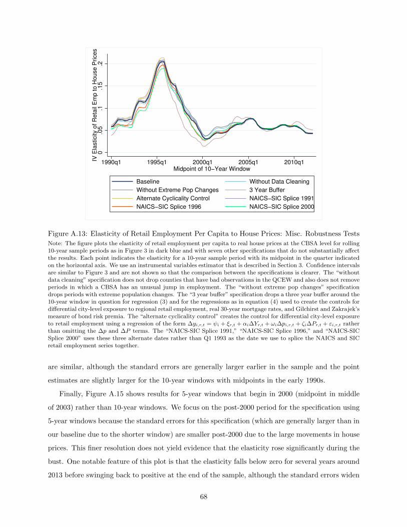
0.0
5.1
.15
.2IV
Ela
sticity o
f R
eta
il E
mp to H
ouse P
rices
1990q1 1995q1 2000q1 2005q1 2010q1Midpoint of 10−Year Window
Baseline Without Data Cleaning
Without Extreme Pop Changes 3 Year Buffer
Alternate Cyclicality Control NAICS−SIC Splice 1991
NAICS−SIC Splice 1996 NAICS−SIC Splice 2000
Figure A.13: Elasticity of Retail Employment Per Capita to House Prices: Misc. Robustness Tests
Note: The figure plots the elasticity of retail employment per capita to real house prices at the CBSA level for rolling10-year sample periods as in Figure 3 in dark blue and with seven other specifications that do not substantially affectthe results. Each point indicates the elasticity for a 10-year sample period with its midpoint in the quarter indicatedon the horizontal axis. We use an instrumental variables estimator that is described in Section 3. Confidence intervalsare similar to Figure 3 and are not shown so that the comparison between the specifications is clearer. The “withoutdata cleaning” specification does not drop counties that have bad observations in the QCEW and also does not removeperiods in which a CBSA has an unusual jump in employment. The “without extreme pop changes” specificationdrops periods with extreme population changes. The “3 year buffer” specification drops a three year buffer around the10-year window in question for regression (3) and for the regressions as in equation (4) used to create the controls fordifferential city-level exposure to regional retail employment, real 30-year mortgage rates, and Gilchirst and Zakrajek’smeasure of bond risk premia. The “alternate cyclicality control” creates the control for differential city-level exposureto retail employment using a regression of the form ∆yi,r,t = ψi + ξr,t + αi∆Yr,t + ωi∆pi,r,t + ζi∆Pr,t + εi,r,t ratherthan omitting the ∆p and ∆P terms. The “NAICS-SIC Splice 1991,” “NAICS-SIC Splice 1996,” and “NAICS-SICSplice 2000” uses these three alternate dates rather than Q1 1993 as the date we use to splice the NAICS and SICretail employment series together.
are similar, although the standard errors are generally larger earlier in the sample and the point
estimates are slightly larger for the 10-year windows with midpoints in the early 1990s.
Finally, Figure A.15 shows results for 5-year windows that begin in 2000 (midpoint in middle
of 2003) rather than 10-year windows. We focus on the post-2000 period for the specification using
5-year windows because the standard errors for this specification (which are generally larger than in
our baseline due to the shorter window) are smaller post-2000 due to the large movements in house
prices. This finer resolution does not yield evidence that the elasticity rose significantly during the
bust. One notable feature of this plot is that the elasticity falls below zero for several years around
2013 before swinging back to positive at the end of the sample, although the standard errors widen
68
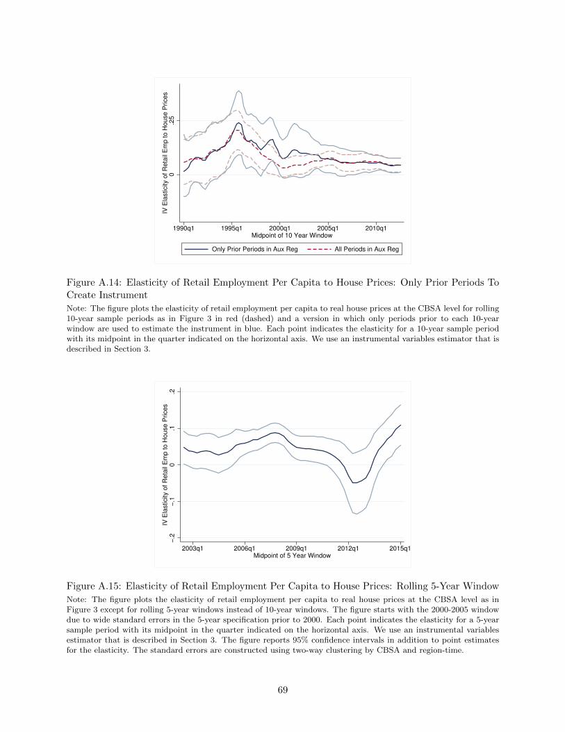
0.2
5IV
Ela
sticity o
f R
eta
il E
mp to H
ouse P
rices
1990q1 1995q1 2000q1 2005q1 2010q1Midpoint of 10 Year Window
Only Prior Periods in Aux Reg All Periods in Aux Reg
Figure A.14: Elasticity of Retail Employment Per Capita to House Prices: Only Prior Periods ToCreate Instrument
Note: The figure plots the elasticity of retail employment per capita to real house prices at the CBSA level for rolling10-year sample periods as in Figure 3 in red (dashed) and a version in which only periods prior to each 10-yearwindow are used to estimate the instrument in blue. Each point indicates the elasticity for a 10-year sample periodwith its midpoint in the quarter indicated on the horizontal axis. We use an instrumental variables estimator that isdescribed in Section 3.
−.2
−.1
0.1
.2IV
Ela
sticity o
f R
eta
il E
mp to H
ouse P
rices
2003q1 2006q1 2009q1 2012q1 2015q1Midpoint of 5 Year Window
Figure A.15: Elasticity of Retail Employment Per Capita to House Prices: Rolling 5-Year Window
Note: The figure plots the elasticity of retail employment per capita to real house prices at the CBSA level as inFigure 3 except for rolling 5-year windows instead of 10-year windows. The figure starts with the 2000-2005 windowdue to wide standard errors in the 5-year specification prior to 2000. Each point indicates the elasticity for a 5-yearsample period with its midpoint in the quarter indicated on the horizontal axis. We use an instrumental variablesestimator that is described in Section 3. The figure reports 95% confidence intervals in addition to point estimatesfor the elasticity. The standard errors are constructed using two-way clustering by CBSA and region-time.
69
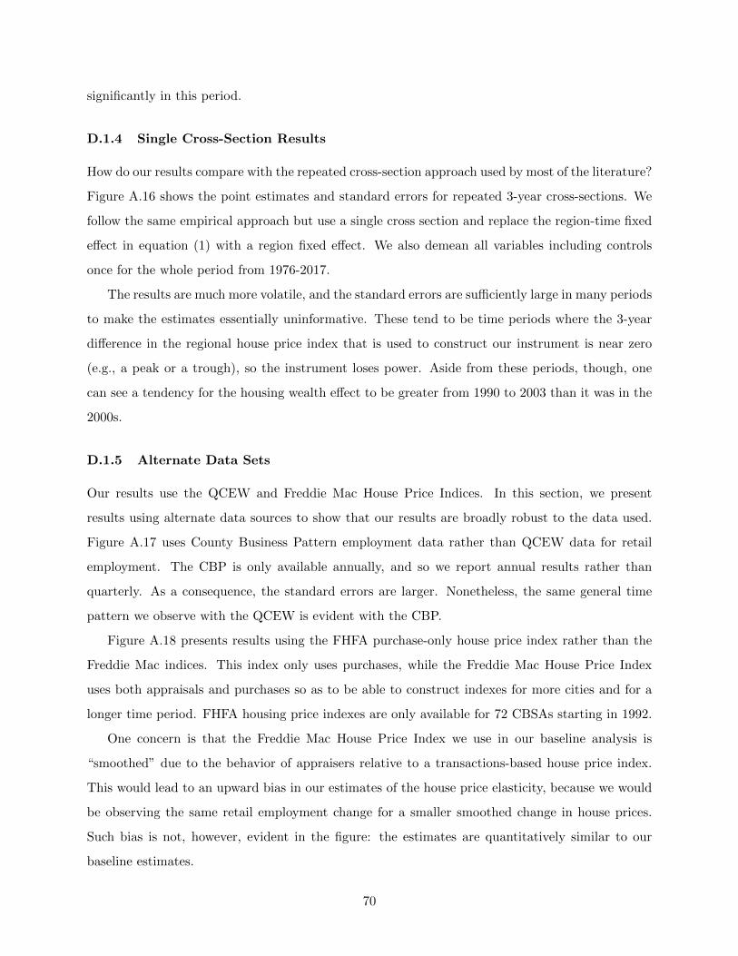
significantly in this period.
D.1.4 Single Cross-Section Results
How do our results compare with the repeated cross-section approach used by most of the literature?
Figure A.16 shows the point estimates and standard errors for repeated 3-year cross-sections. We
follow the same empirical approach but use a single cross section and replace the region-time fixed
effect in equation (1) with a region fixed effect. We also demean all variables including controls
once for the whole period from 1976-2017.
The results are much more volatile, and the standard errors are sufficiently large in many periods
to make the estimates essentially uninformative. These tend to be time periods where the 3-year
difference in the regional house price index that is used to construct our instrument is near zero
(e.g., a peak or a trough), so the instrument loses power. Aside from these periods, though, one
can see a tendency for the housing wealth effect to be greater from 1990 to 2003 than it was in the
2000s.
D.1.5 Alternate Data Sets
Our results use the QCEW and Freddie Mac House Price Indices. In this section, we present
results using alternate data sources to show that our results are broadly robust to the data used.
Figure A.17 uses County Business Pattern employment data rather than QCEW data for retail
employment. The CBP is only available annually, and so we report annual results rather than
quarterly. As a consequence, the standard errors are larger. Nonetheless, the same general time
pattern we observe with the QCEW is evident with the CBP.
Figure A.18 presents results using the FHFA purchase-only house price index rather than the
Freddie Mac indices. This index only uses purchases, while the Freddie Mac House Price Index
uses both appraisals and purchases so as to be able to construct indexes for more cities and for a
longer time period. FHFA housing price indexes are only available for 72 CBSAs starting in 1992.
One concern is that the Freddie Mac House Price Index we use in our baseline analysis is
“smoothed” due to the behavior of appraisers relative to a transactions-based house price index.
This would lead to an upward bias in our estimates of the house price elasticity, because we would
be observing the same retail employment change for a smaller smoothed change in house prices.
Such bias is not, however, evident in the figure: the estimates are quantitatively similar to our
baseline estimates.
70
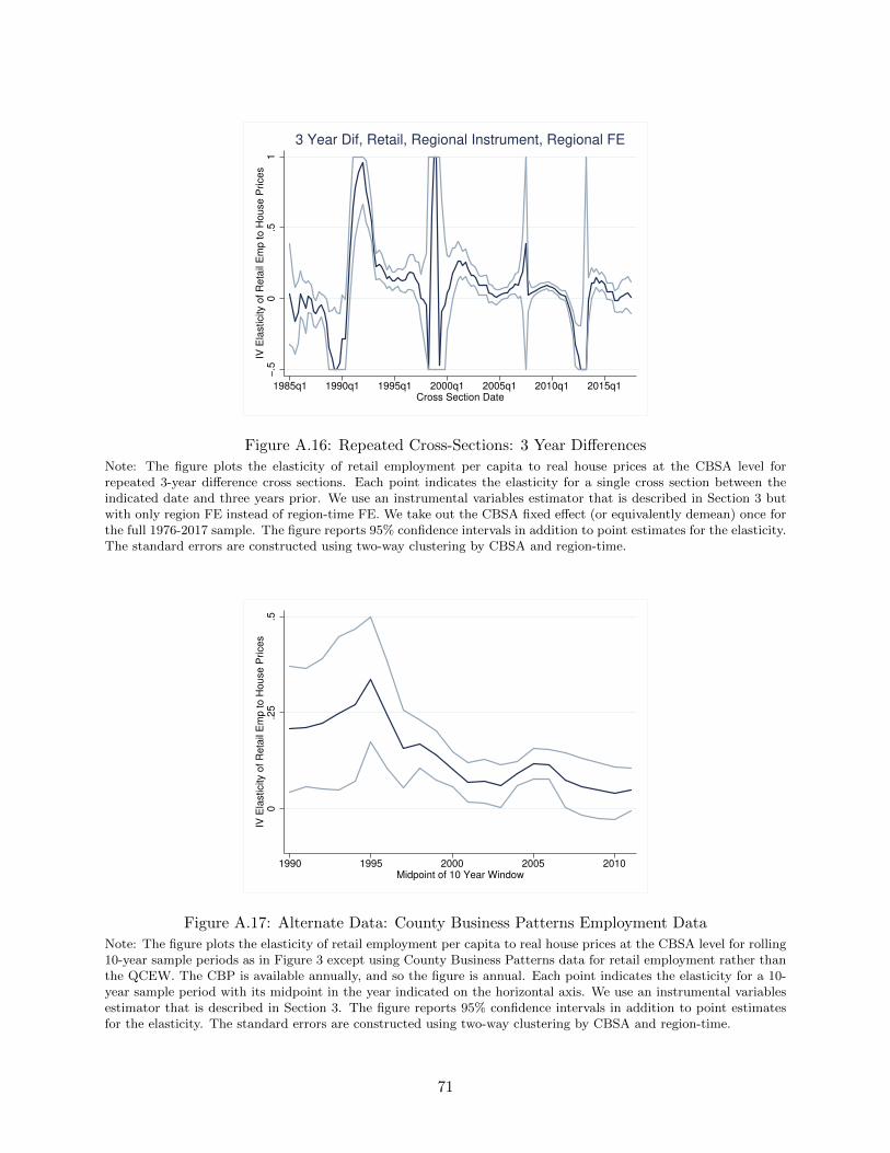
−.5
0.5
1IV
Ela
sticity o
f R
eta
il E
mp to H
ouse P
rices
1985q1 1990q1 1995q1 2000q1 2005q1 2010q1 2015q1Cross Section Date
3 Year Dif, Retail, Regional Instrument, Regional FE
Figure A.16: Repeated Cross-Sections: 3 Year Differences
Note: The figure plots the elasticity of retail employment per capita to real house prices at the CBSA level forrepeated 3-year difference cross sections. Each point indicates the elasticity for a single cross section between theindicated date and three years prior. We use an instrumental variables estimator that is described in Section 3 butwith only region FE instead of region-time FE. We take out the CBSA fixed effect (or equivalently demean) once forthe full 1976-2017 sample. The figure reports 95% confidence intervals in addition to point estimates for the elasticity.The standard errors are constructed using two-way clustering by CBSA and region-time.
0.2
5.5
IV E
lasticity o
f R
eta
il E
mp to H
ouse P
rices
1990 1995 2000 2005 2010Midpoint of 10 Year Window
Figure A.17: Alternate Data: County Business Patterns Employment Data
Note: The figure plots the elasticity of retail employment per capita to real house prices at the CBSA level for rolling10-year sample periods as in Figure 3 except using County Business Patterns data for retail employment rather thanthe QCEW. The CBP is available annually, and so the figure is annual. Each point indicates the elasticity for a 10-year sample period with its midpoint in the year indicated on the horizontal axis. We use an instrumental variablesestimator that is described in Section 3. The figure reports 95% confidence intervals in addition to point estimatesfor the elasticity. The standard errors are constructed using two-way clustering by CBSA and region-time.
71
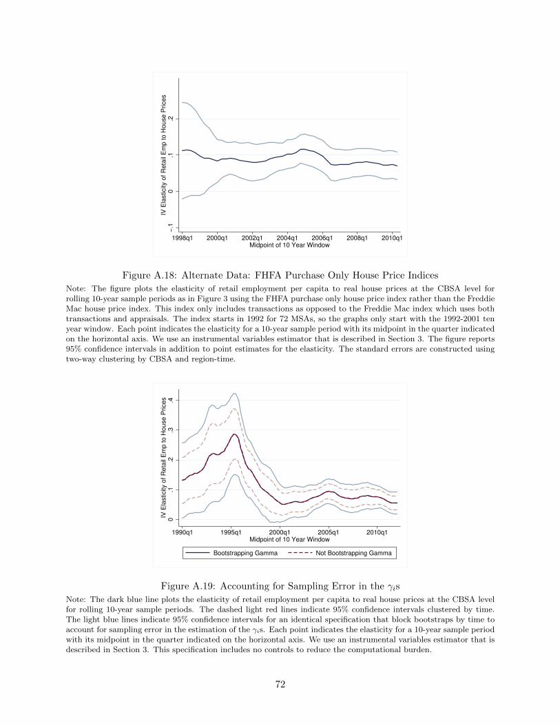
−.1
0.1
.2IV
Ela
sticity o
f R
eta
il E
mp to H
ouse P
rices
1998q1 2000q1 2002q1 2004q1 2006q1 2008q1 2010q1Midpoint of 10 Year Window
Figure A.18: Alternate Data: FHFA Purchase Only House Price Indices
Note: The figure plots the elasticity of retail employment per capita to real house prices at the CBSA level forrolling 10-year sample periods as in Figure 3 using the FHFA purchase only house price index rather than the FreddieMac house price index. This index only includes transactions as opposed to the Freddie Mac index which uses bothtransactions and appraisals. The index starts in 1992 for 72 MSAs, so the graphs only start with the 1992-2001 tenyear window. Each point indicates the elasticity for a 10-year sample period with its midpoint in the quarter indicatedon the horizontal axis. We use an instrumental variables estimator that is described in Section 3. The figure reports95% confidence intervals in addition to point estimates for the elasticity. The standard errors are constructed usingtwo-way clustering by CBSA and region-time.
0.1
.2.3
.4IV
Ela
sticity o
f R
eta
il E
mp to H
ouse P
rices
1990q1 1995q1 2000q1 2005q1 2010q1Midpoint of 10 Year Window
Bootstrapping Gamma Not Bootstrapping Gamma
Figure A.19: Accounting for Sampling Error in the γis
Note: The dark blue line plots the elasticity of retail employment per capita to real house prices at the CBSA levelfor rolling 10-year sample periods. The dashed light red lines indicate 95% confidence intervals clustered by time.The light blue lines indicate 95% confidence intervals for an identical specification that block bootstraps by time toaccount for sampling error in the estimation of the γis. Each point indicates the elasticity for a 10-year sample periodwith its midpoint in the quarter indicated on the horizontal axis. We use an instrumental variables estimator that isdescribed in Section 3. This specification includes no controls to reduce the computational burden.
72
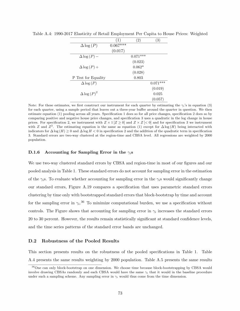
Table A.4: 1990-2017 Elasticity of Retail Employment Per Capita to House Prices: Weighted
(1) (2) (3)
∆ log (P ) 0.067***(0.017)
∆ log (P )− 0.071***
(0.023)
∆ log (P ) + 0.062*
(0.028)
P Test for Equality 0.803
∆ log (P ) 0.071***
(0.019)
∆ log (P )2
0.025
(0.057)
Note: For these estimates, we first construct our instrument for each quarter by estimating the γi’s in equation (3)for each quarter, using a sample period that leaves out a three-year buffer around the quarter in question. We thenestimate equation (1) pooling across all years. Specification 1 does so for all price changes, specification 2 does so bycomparing positive and negative house price changes, and specification 3 uses a quadratic in the log change in houseprices. For specification 2, we instrument with Z × 1 [Z ≥ 0] and Z × Z [< 0] and for specification 3 we instrumentwith Z and Z2. The estimating equation is the same as equation (1) except for ∆ log (H) being interacted withindicators for ∆ log (H) ≥ 0 and ∆ logH < 0 in specification 2 and the addition of the quadratic term in specification3. Standard errors are two-way clustered at the region-time and CBSA level. All regressions are weighted by 2000population.
D.1.6 Accounting for Sampling Error in the γis
We use two-way clustered standard errors by CBSA and region-time in most of our figures and our
pooled analysis in Table 1. These standard errors do not account for sampling error in the estimation
of the γis. To evaluate whether accounting for sampling error in the γis would significantly change
our standard errors, Figure A.19 compares a specification that uses parametric standard errors
clustering by time only with bootstrapped standard errors that block-bootstrap by time and account
for the sampling error in γi.36 To minimize computational burden, we use a specification without
controls. The Figure shows that accounting for sampling error in γi increases the standard errors
20 to 30 percent. However, the results remain statistically significant at standard confidence levels,
and the time series patterns of the standard error bands are unchanged.
D.2 Robustness of the Pooled Results
This section presents results on the robustness of the pooled specifications in Table 1. Table
A.4 presents the same results weighting by 2000 population. Table A.5 presents the same results
36One can only block-bootstrap on one dimension. We choose time because block-bootstrapping by CBSA wouldinvolve drawing CBSAs randomly and each CBSA would have the same γi that it would in the baseline procedureunder such a sampling scheme. Any sampling error in γi would thus come from the time dimension.
73

Table A.5: 1990-2017 Elasticity of Retail Employment Per Capita to House Prices: No Controls
(1) (2) (3)
∆ log (P ) 0.088***(0.012)
∆ log (P )− 0.101***
(0.018)
∆ log (P ) + 0.070***
(0.017)
P Test for Equality 0.215
∆ log (P ) 0.088***
(0.013)
∆ log (P )2
0.000
(0.037)
Note: For these estimates, we first construct our instrument for each quarter by estimating the γi’s in equation (3)for each quarter, using a sample period that leaves out a three-year buffer around the quarter in question. We thenestimate equation (1) pooling across all years. Specification 1 does so for all price changes, specification 2 does so bycomparing positive and negative house price changes, and specification 3 uses a quadratic in the log change in houseprices. For specification 2, we instrument with Z × 1 [Z ≥ 0] and Z × Z [< 0] and for specification 3 we instrumentwith Z and Z2. The estimating equation is the same as equation (1) except for ∆ log (H) being interacted withindicators for ∆ log (H) ≥ 0 and ∆ logH < 0 in specification 2 and the addition of the quadratic term in specification3. Standard errors are two-way clustered at the region-time and CBSA level. All regressions do not include thestandard controls in our baseline specification.
without controls. The point estimates for the weighted regression are somewhat lower, and the
point estimates for the version without controls are somewhat higher. In no specification do we
find any strong evidence of a boom-bust asymmetry.
E Model Extensions and Robustness
This section analyzes the robustness of the model results to various extensions and relaxations of
assumptions. It is organized as follows:
E.1 Linearity and Interaction Effects
E.2 Changes to β
E.3 Changes in Credit Constraints
E.4 Interest Rate Changes
E.5 Rental Cost of Housing
E.6 Short-Term Debt
74
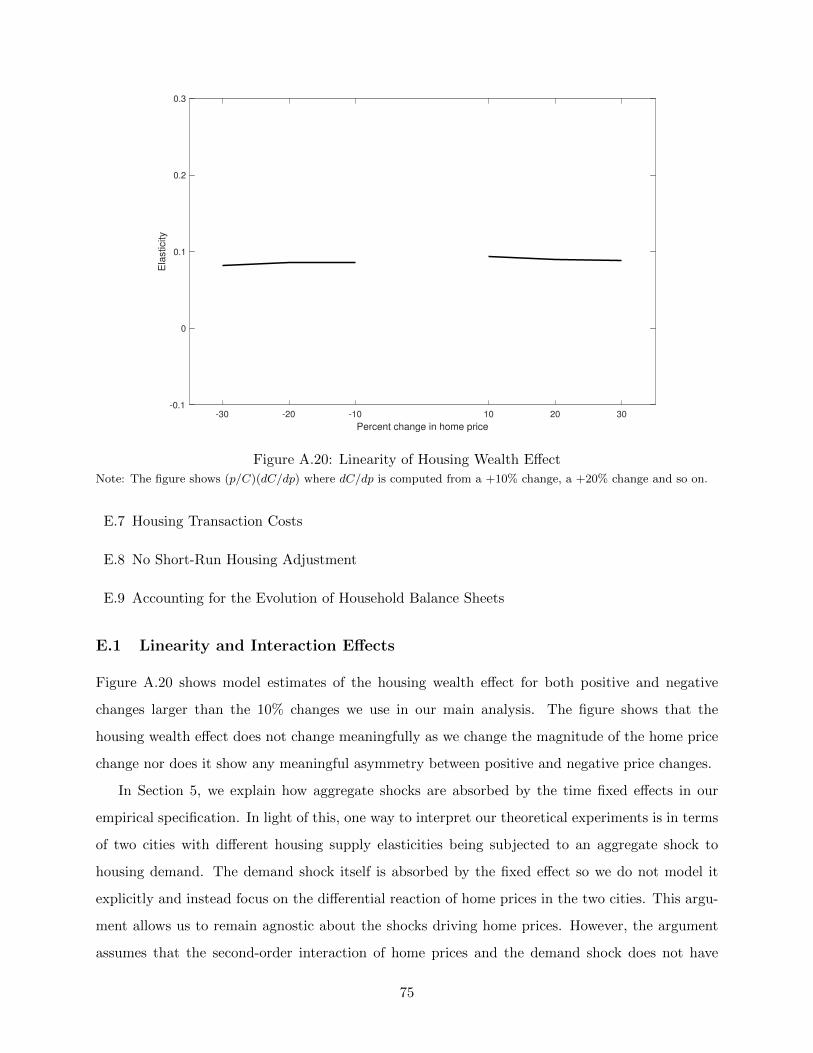
-30 -20 -10 10 20 30
Percent change in home price
-0.1
0
0.1
0.2
0.3
Ela
sticity
Figure A.20: Linearity of Housing Wealth Effect
Note: The figure shows (p/C)(dC/dp) where dC/dp is computed from a +10% change, a +20% change and so on.
E.7 Housing Transaction Costs
E.8 No Short-Run Housing Adjustment
E.9 Accounting for the Evolution of Household Balance Sheets
E.1 Linearity and Interaction Effects
Figure A.20 shows model estimates of the housing wealth effect for both positive and negative
changes larger than the 10% changes we use in our main analysis. The figure shows that the
housing wealth effect does not change meaningfully as we change the magnitude of the home price
change nor does it show any meaningful asymmetry between positive and negative price changes.
In Section 5, we explain how aggregate shocks are absorbed by the time fixed effects in our
empirical specification. In light of this, one way to interpret our theoretical experiments is in terms
of two cities with different housing supply elasticities being subjected to an aggregate shock to
housing demand. The demand shock itself is absorbed by the fixed effect so we do not model it
explicitly and instead focus on the differential reaction of home prices in the two cities. This argu-
ment allows us to remain agnostic about the shocks driving home prices. However, the argument
assumes that the second-order interaction of home prices and the demand shock does not have
75
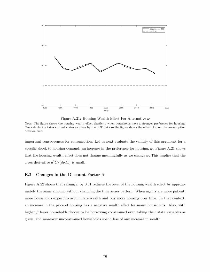
1980 1985 1990 1995 2000 2005 2010 2015 2020
Year
-0.1
0
0.1
0.2
0.3
Baseline: = 0.08
= 0.10
Figure A.21: Housing Wealth Effect For Alternative ω
Note: The figure shows the housing wealth effect elasticity when households have a stronger preference for housing.Our calculation takes current states as given by the SCF data so the figure shows the effect of ω on the consumptiondecision rule.
important consequences for consumption. Let us next evaluate the validity of this argument for a
specific shock to housing demand: an increase in the preference for housing, ω. Figure A.21 shows
that the housing wealth effect does not change meaningfully as we change ω. This implies that the
cross derivative d2C/(dpdω) is small.
E.2 Changes in the Discount Factor β
Figure A.22 shows that raising β by 0.01 reduces the level of the housing wealth effect by approxi-
mately the same amount without changing the time series pattern. When agents are more patient,
more households expect to accumulate wealth and buy more housing over time. In that context,
an increase in the price of housing has a negative wealth effect for many households. Also, with
higher β fewer households choose to be borrowing constrained even taking their state variables as
given, and moreover unconstrained households spend less of any increase in wealth.
76
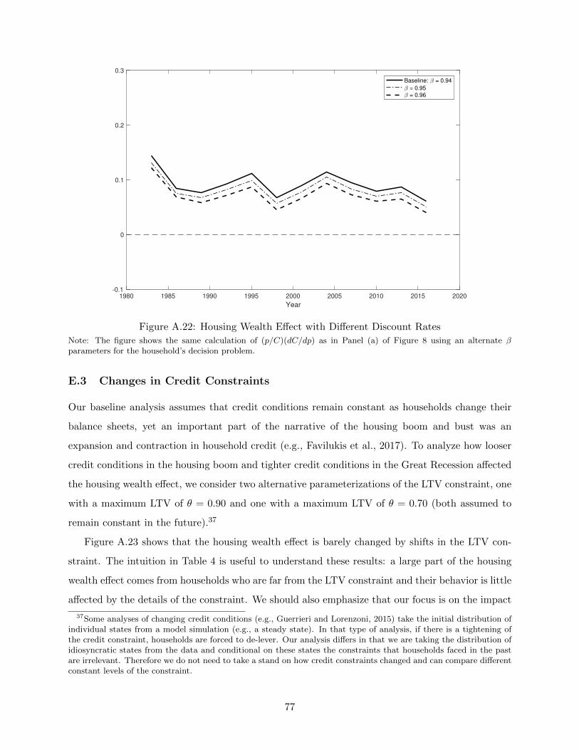
1980 1985 1990 1995 2000 2005 2010 2015 2020
Year
-0.1
0
0.1
0.2
0.3
Baseline: = 0.94
= 0.95
= 0.96
Figure A.22: Housing Wealth Effect with Different Discount Rates
Note: The figure shows the same calculation of (p/C)(dC/dp) as in Panel (a) of Figure 8 using an alternate βparameters for the household’s decision problem.
E.3 Changes in Credit Constraints
Our baseline analysis assumes that credit conditions remain constant as households change their
balance sheets, yet an important part of the narrative of the housing boom and bust was an
expansion and contraction in household credit (e.g., Favilukis et al., 2017). To analyze how looser
credit conditions in the housing boom and tighter credit conditions in the Great Recession affected
the housing wealth effect, we consider two alternative parameterizations of the LTV constraint, one
with a maximum LTV of θ = 0.90 and one with a maximum LTV of θ = 0.70 (both assumed to
remain constant in the future).37
Figure A.23 shows that the housing wealth effect is barely changed by shifts in the LTV con-
straint. The intuition in Table 4 is useful to understand these results: a large part of the housing
wealth effect comes from households who are far from the LTV constraint and their behavior is little
affected by the details of the constraint. We should also emphasize that our focus is on the impact
37Some analyses of changing credit conditions (e.g., Guerrieri and Lorenzoni, 2015) take the initial distribution ofindividual states from a model simulation (e.g., a steady state). In that type of analysis, if there is a tightening ofthe credit constraint, households are forced to de-lever. Our analysis differs in that we are taking the distribution ofidiosyncratic states from the data and conditional on these states the constraints that households faced in the pastare irrelevant. Therefore we do not need to take a stand on how credit constraints changed and can compare differentconstant levels of the constraint.
77
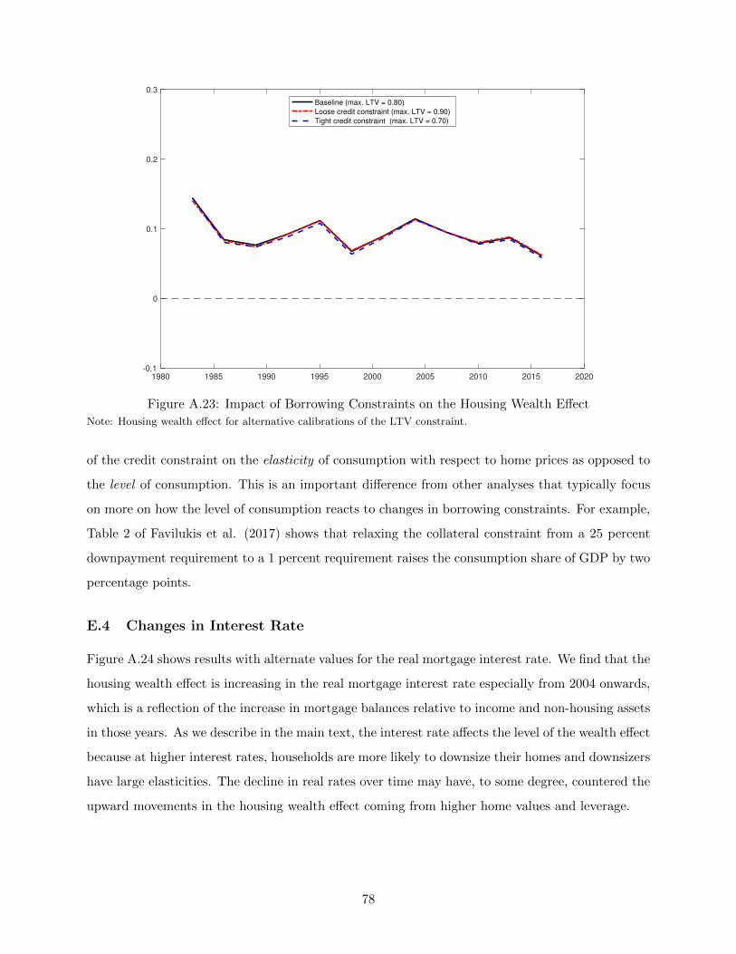
1980 1985 1990 1995 2000 2005 2010 2015 2020-0.1
0
0.1
0.2
0.3
Baseline (max. LTV = 0.80)
Loose credit constraint (max. LTV = 0.90)
Tight credit constraint (max. LTV = 0.70)
Figure A.23: Impact of Borrowing Constraints on the Housing Wealth Effect
Note: Housing wealth effect for alternative calibrations of the LTV constraint.
of the credit constraint on the elasticity of consumption with respect to home prices as opposed to
the level of consumption. This is an important difference from other analyses that typically focus
on more on how the level of consumption reacts to changes in borrowing constraints. For example,
Table 2 of Favilukis et al. (2017) shows that relaxing the collateral constraint from a 25 percent
downpayment requirement to a 1 percent requirement raises the consumption share of GDP by two
percentage points.
E.4 Changes in Interest Rate
Figure A.24 shows results with alternate values for the real mortgage interest rate. We find that the
housing wealth effect is increasing in the real mortgage interest rate especially from 2004 onwards,
which is a reflection of the increase in mortgage balances relative to income and non-housing assets
in those years. As we describe in the main text, the interest rate affects the level of the wealth effect
because at higher interest rates, households are more likely to downsize their homes and downsizers
have large elasticities. The decline in real rates over time may have, to some degree, countered the
upward movements in the housing wealth effect coming from higher home values and leverage.
78
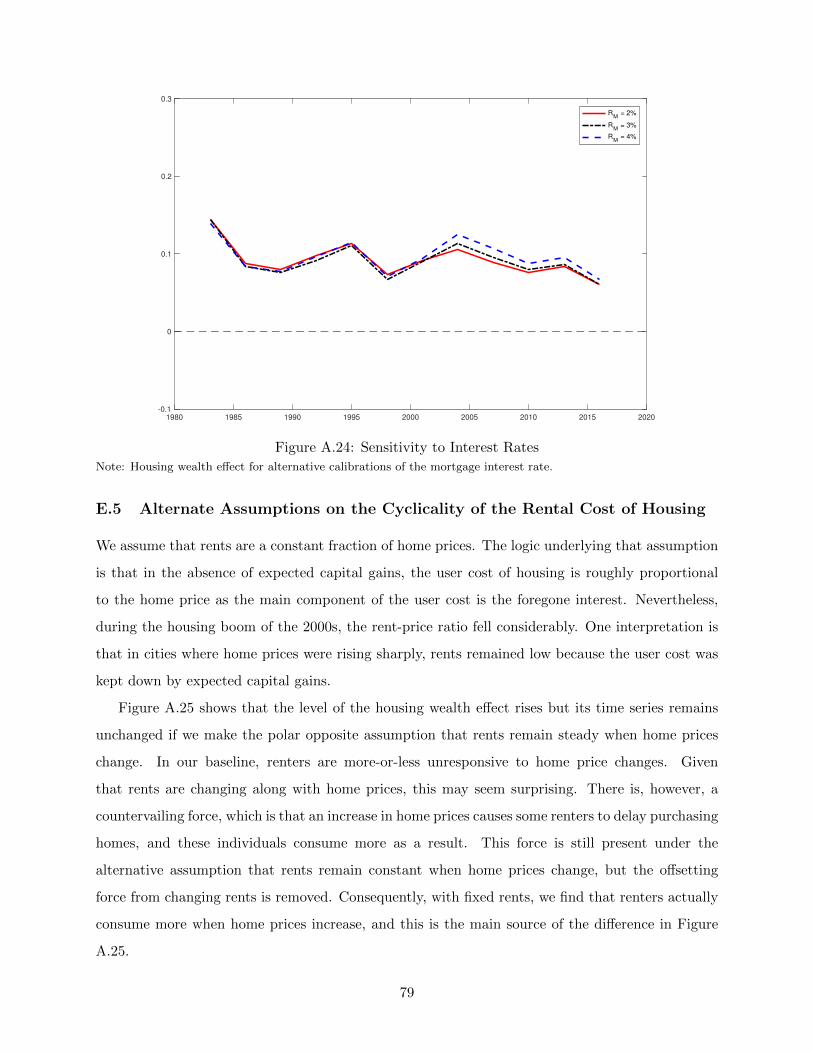
1980 1985 1990 1995 2000 2005 2010 2015 2020
-0.1
0
0.1
0.2
0.3
RM
= 2%
RM
= 3%
RM
= 4%
Figure A.24: Sensitivity to Interest Rates
Note: Housing wealth effect for alternative calibrations of the mortgage interest rate.
E.5 Alternate Assumptions on the Cyclicality of the Rental Cost of Housing
We assume that rents are a constant fraction of home prices. The logic underlying that assumption
is that in the absence of expected capital gains, the user cost of housing is roughly proportional
to the home price as the main component of the user cost is the foregone interest. Nevertheless,
during the housing boom of the 2000s, the rent-price ratio fell considerably. One interpretation is
that in cities where home prices were rising sharply, rents remained low because the user cost was
kept down by expected capital gains.
Figure A.25 shows that the level of the housing wealth effect rises but its time series remains
unchanged if we make the polar opposite assumption that rents remain steady when home prices
change. In our baseline, renters are more-or-less unresponsive to home price changes. Given
that rents are changing along with home prices, this may seem surprising. There is, however, a
countervailing force, which is that an increase in home prices causes some renters to delay purchasing
homes, and these individuals consume more as a result. This force is still present under the
alternative assumption that rents remain constant when home prices change, but the offsetting
force from changing rents is removed. Consequently, with fixed rents, we find that renters actually
consume more when home prices increase, and this is the main source of the difference in Figure
A.25.
79
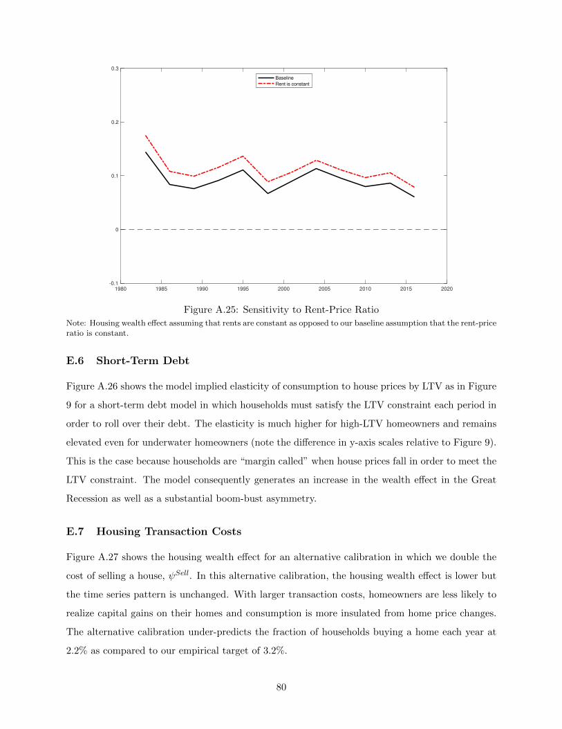
1980 1985 1990 1995 2000 2005 2010 2015 2020
-0.1
0
0.1
0.2
0.3
Baseline
Rent is constant
Figure A.25: Sensitivity to Rent-Price Ratio
Note: Housing wealth effect assuming that rents are constant as opposed to our baseline assumption that the rent-priceratio is constant.
E.6 Short-Term Debt
Figure A.26 shows the model implied elasticity of consumption to house prices by LTV as in Figure
9 for a short-term debt model in which households must satisfy the LTV constraint each period in
order to roll over their debt. The elasticity is much higher for high-LTV homeowners and remains
elevated even for underwater homeowners (note the difference in y-axis scales relative to Figure 9).
This is the case because households are “margin called” when house prices fall in order to meet the
LTV constraint. The model consequently generates an increase in the wealth effect in the Great
Recession as well as a substantial boom-bust asymmetry.
E.7 Housing Transaction Costs
Figure A.27 shows the housing wealth effect for an alternative calibration in which we double the
cost of selling a house, ψSell. In this alternative calibration, the housing wealth effect is lower but
the time series pattern is unchanged. With larger transaction costs, homeowners are less likely to
realize capital gains on their homes and consumption is more insulated from home price changes.
The alternative calibration under-predicts the fraction of households buying a home each year at
2.2% as compared to our empirical target of 3.2%.
80
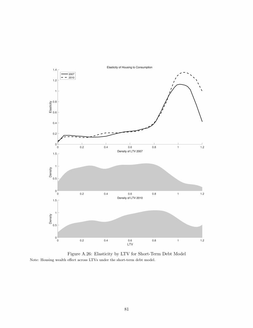
0 0.2 0.4 0.6 0.8 1 1.20
0.2
0.4
0.6
0.8
1
1.2
1.4
Ela
sticity
Elasticity of Housing to Consumption
2007
2010
0 0.2 0.4 0.6 0.8 1 1.20
0.5
1
1.5
De
nsity
Density of LTV 2007
0 0.2 0.4 0.6 0.8 1 1.2
LTV
0
0.5
1
1.5
De
nsity
Density of LTV 2010
Figure A.26: Elasticity by LTV for Short-Term Debt Model
Note: Housing wealth effect across LTVs under the short-term debt model.
81
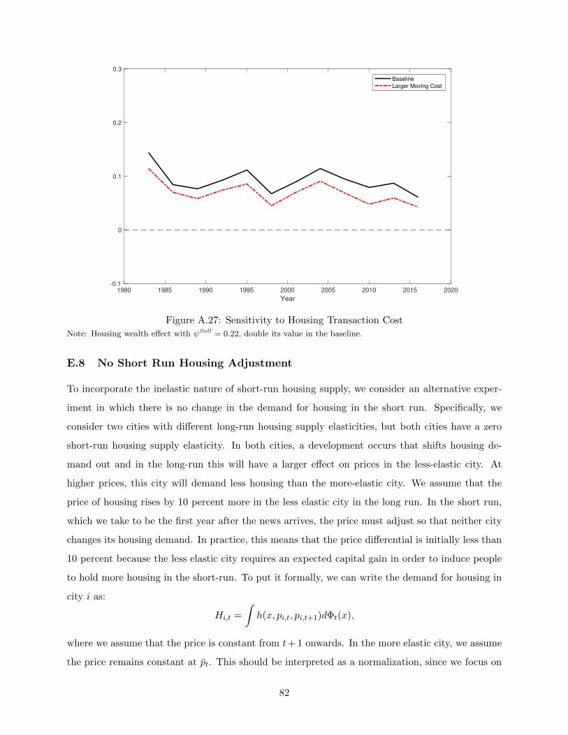
1980 1985 1990 1995 2000 2005 2010 2015 2020
Year
-0.1
0
0.1
0.2
0.3
Baseline
Larger Moving Cost
Figure A.27: Sensitivity to Housing Transaction Cost
Note: Housing wealth effect with ψSell = 0.22, double its value in the baseline.
E.8 No Short Run Housing Adjustment
To incorporate the inelastic nature of short-run housing supply, we consider an alternative exper-
iment in which there is no change in the demand for housing in the short run. Specifically, we
consider two cities with different long-run housing supply elasticities, but both cities have a zero
short-run housing supply elasticity. In both cities, a development occurs that shifts housing de-
mand out and in the long-run this will have a larger effect on prices in the less-elastic city. At
higher prices, this city will demand less housing than the more-elastic city. We assume that the
price of housing rises by 10 percent more in the less elastic city in the long run. In the short run,
which we take to be the first year after the news arrives, the price must adjust so that neither city
changes its housing demand. In practice, this means that the price differential is initially less than
10 percent because the less elastic city requires an expected capital gain in order to induce people
to hold more housing in the short-run. To put it formally, we can write the demand for housing in
city i as:
Hi,t =
∫h(x, pi,t, pi,t+1)dΦt(x),
where we assume that the price is constant from t+ 1 onwards. In the more elastic city, we assume
the price remains constant at pt. This should be interpreted as a normalization, since we focus on
82
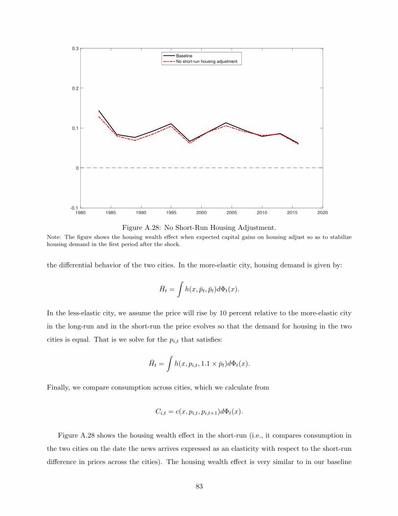
1980 1985 1990 1995 2000 2005 2010 2015 2020-0.1
0
0.1
0.2
0.3
Baseline
No short-run housing adjustment
Figure A.28: No Short-Run Housing Adjustment.
Note: The figure shows the housing wealth effect when expected capital gains on housing adjust so as to stabilizehousing demand in the first period after the shock.
the differential behavior of the two cities. In the more-elastic city, housing demand is given by:
Ht =
∫h(x, pt, pt)dΦt(x).
In the less-elastic city, we assume the price will rise by 10 percent relative to the more-elastic city
in the long-run and in the short-run the price evolves so that the demand for housing in the two
cities is equal. That is we solve for the pi,t that satisfies:
Ht =
∫h(x, pi,t, 1.1× pt)dΦt(x).
Finally, we compare consumption across cities, which we calculate from
Ci,t = c(x, pi,t, pi,t+1)dΦt(x).
Figure A.28 shows the housing wealth effect in the short-run (i.e., it compares consumption in
the two cities on the date the news arrives expressed as an elasticity with respect to the short-run
difference in prices across the cities). The housing wealth effect is very similar to in our baseline
83
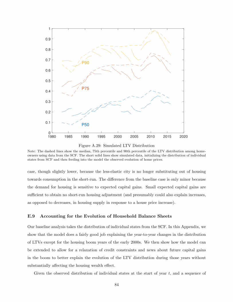
1980 1985 1990 1995 2000 2005 2010 2015 2020
0
0.1
0.2
0.3
0.4
0.5
0.6
0.7
0.8
0.9
1
P50
P75
P90
Figure A.29: Simulated LTV Distribution
Note: The dashed lines show the median, 75th percentile and 90th percentile of the LTV distribution among home-owners using data from the SCF. The short solid lines show simulated data, initializing the distribution of individualstates from SCF and then feeding into the model the observed evolution of home prices.
case, though slightly lower, because the less-elastic city is no longer substituting out of housing
towards consumption in the short-run. The difference from the baseline case is only minor because
the demand for housing is sensitive to expected capital gains. Small expected capital gains are
sufficient to obtain no short-run housing adjustment (and presumably could also explain increases,
as opposed to decreases, in housing supply in response to a house price increase).
E.9 Accounting for the Evolution of Household Balance Sheets
Our baseline analysis takes the distribution of individual states from the SCF. In this Appendix, we
show that the model does a fairly good job explaining the year-to-year changes in the distribution
of LTVs except for the housing boom years of the early 2000s. We then show how the model can
be extended to allow for a relaxation of credit constraints and news about future capital gains
in the boom to better explain the evolution of the LTV distribution during those years without
substantially affecting the housing wealth effect.
Given the observed distribution of individual states at the start of year t, and a sequence of
84
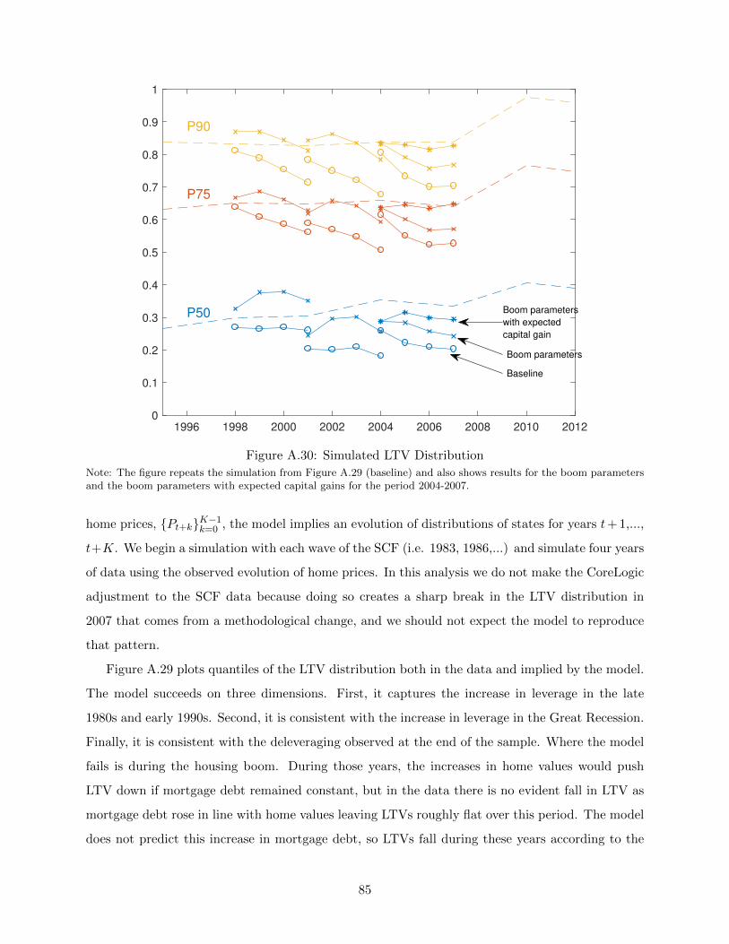
1996 1998 2000 2002 2004 2006 2008 2010 20120
0.1
0.2
0.3
0.4
0.5
0.6
0.7
0.8
0.9
1
P50
P75
P90
Baseline
Boom parameters
Boom parameters
with expected
capital gain
Figure A.30: Simulated LTV Distribution
Note: The figure repeats the simulation from Figure A.29 (baseline) and also shows results for the boom parametersand the boom parameters with expected capital gains for the period 2004-2007.
home prices, Pt+kK−1k=0 , the model implies an evolution of distributions of states for years t+ 1,...,
t+K. We begin a simulation with each wave of the SCF (i.e. 1983, 1986,...) and simulate four years
of data using the observed evolution of home prices. In this analysis we do not make the CoreLogic
adjustment to the SCF data because doing so creates a sharp break in the LTV distribution in
2007 that comes from a methodological change, and we should not expect the model to reproduce
that pattern.
Figure A.29 plots quantiles of the LTV distribution both in the data and implied by the model.
The model succeeds on three dimensions. First, it captures the increase in leverage in the late
1980s and early 1990s. Second, it is consistent with the increase in leverage in the Great Recession.
Finally, it is consistent with the deleveraging observed at the end of the sample. Where the model
fails is during the housing boom. During those years, the increases in home values would push
LTV down if mortgage debt remained constant, but in the data there is no evident fall in LTV as
mortgage debt rose in line with home values leaving LTVs roughly flat over this period. The model
does not predict this increase in mortgage debt, so LTVs fall during these years according to the
85
model.
Next we introduce the “boom” parameterization described in the main text that differs from
the baseline parameters in that the LTV limit increases from 80 percent to 95 percent and refi-
nancing is free. We use this calibration to simulate the years 1998 to 2007. One interpretation of
free refinancing is that the decline in mortgage interest rates following the 2001 recession created
strong incentives for refinancing that offset the transaction costs of doing so. Second, we allow for
expectations of capital gains to be nonzero. Specifically, we assume the one-year expected capital
gain rises from 0 to 2 percent in a linear fashion from 2004 to 2007. That is, in 2004 people expect
home prices to be constant going forward and in 2007 they expect a 2 percent appreciation in 2008
followed by constant prices thereafter. Expected capital gains increase leverage for two reasons:
first, homeowners feel richer and increase consumption due to a wealth effect and, second, the
expected return on housing lowers the user cost of housing and prompts an increase in the demand
for housing financed with mortgage debt.
Figure A.30 shows that these changes to the model give a fairly good account of the LTV distri-
bution during the housing boom. As described in the main text, these changes do not significantly
alter the housing wealth effect. Indeed, in 2007, the baseline parameters lead to a housing wealth
effect of 0.095, the boom parameters lead to 0.098, and the boom parameters with the expected
capital gain leads to 0.114.
86