Housing Demand and Household Saving Rates in China:

Evidence from a Housing Reform

Binkai Chen Xi Yang Ninghua Zhong*

March 30, 2019

Abstract: China’s urban household saving rate has increased markedly since the mid-

1990s, accompanied by a dramatic increase in home ownership. Is there a causal link

between those two phenomena? This paper takes advantage of a unique natural exper-

iment in China, which reformed the nationwide employer-based public housing system

in 1998. This reform created an exogenous variation in housing demand among urban

households. Using a difference-in-differences estimation strategy, we find evidence that

the reform increased household saving rates during the reform period (1998-2001) by

shifting the cost of housing services from the state to households. We also provide

evidence suggesting that the 1998 housing reform affects household saving behaviors

even after the reform period (2002-2009).

Keywords: China, urban housing reform, household saving

JEL Classification: D14, D12, E21

*Binkai Chen, School of Economics, Central University of Finance and Economics, chen-binkai@cufe.edu.cn; Xi Yang, Department of Economics, University of North Texas, xi.yang@unt.edu;Ninghua Zhong, School of Economics and Management, Tongji University, ninghua.zhong@gmail.com.We would like to thank Siqi Zheng, Junfu Zhang, Shihe Fu, and seminar participants at the 2017American Economic Association session “International Real Estate” and the 2017 Chinese EconomistSociety annual conference for their valuable suggestions. We would also like to thank seminar partic-ipants at Texas A&M University, Beijing University, Central University of Finance and Economics,and Tongji University for their helpful comments.

1 Introduction

In the past few decades, the Chinese housing market has dramatically changed. Accord-

ing to the Chinese Urban Household Survey (UHS), the home ownership rate among

urban households was around 20 percent in the early 1990s, when most of the urban

houses were publicly owned. The rate climbed sharply after 1998 and has reached 90

percent in 2009 (Figure 1), which is among the highest in the world. By comparison,

in 2010 the American home ownership rate was only 65.1 percent according to the U.S.

Census Bureau. Such a rapid privatization of the housing market was unprecedented in

Chinese history. During the same period, the average floor area per capita of Chinese

households tripled, from 13 square meters in 1992 to 32 square meters in 2009 (Ta-

ble A1), which indicates significant improvement in living conditions in less than two

decades. This increased housing demand led to soaring prices; housing prices almost

tripled in China’s major cities between 2000 and 2009 (?). As suggested by ?, an 8 to

10 the price-to-income ratio has been reached in major Chinese cities.

Despite such dramatic changes in the housing market, very little is known about

their consequences. This paper fills the gap by linking China’s volatile housing market

with its economic imbalance, especially the country’s unusually high saving rates. China

has witnessed a significant increase in savings rates in the past two decades, with

household saving as a share of disposable income nearly doubling, from 16 percent in

1992 to 30 percent in 2009. This increase resulted in a large current account surplus,

which is considered a major contributor to global macroeconomic imbalances and a

trigger of the recent global financial crisis (?). From a theoretical perspective, the

rising household saving rate seems puzzling because it was accompanied by a rapid

growth in household income; the permanent income hypothesis (PIH) theory suggests

that consumption instead of saving should increase with income. Both the importance

of understanding global current account imbalances and the theoretical conflict have

motivated a growing body of research into this unusual saving behavior. Various reasons

have been given to explain the ”Chinese saving puzzle,” including an aging population,

lack of social safety nets, precautionary saving motives, an underdeveloped financial

market, and a cultural tradition of thrift (???).

Rising housing demand has been mentioned as one of the explanations behind

rising saving rates; however, current evidence on this mechanism is merely descriptive

and suggestive. For example, ? mention that the rising private burden of housing

1

expenditure appears to have created new motives for saving. ? argue that families

with sons tend to save more for buying a house to improve their sons’ competitiveness

in the marriage market. The main challenge of identifying and quantifying the causal

effects of housing expenditures on household saving is the endogenous problem, because

unobserved abilities or preferences could increase housing expenditure and household

savings simultaneously, which creates a spurious correlation.

In this paper, we deal with the endogenous problem by taking advantage of a

unique natural experiment in China that reformed the employer-provided public housing

system in 1998 and, thus, created an exogenous variation in housing demand among

urban households. Before the reform, the majority of urban residents worked for a state-

owned enterprise and were living in public housing units provided by their employers

with zero or highly subsidized rents.1 To transform the public housing system into

a market-based system, the reform abolished the provision of public housing across

the nation, which created sudden and unexpected changes in housing demand among

urban households. Before the reform, public-sector employees who lived in houses that

lacked essential facilities expected their employers to help them improve their living

conditions by allocating them a public house, so they did not need to save much. The

1998 reform eliminated this possibility. Now the only way for employees to improve

their living conditions was to buy a private house on the market, which was usually

expensive and forced them to increase their saving. In a sense, this reform acted like a

negative wealth shock for those households. In contrast, for the public-sector employees

who already lived in good-quality public housing units, the 1998 reform allowed them

to purchase their houses at below-market prices. Because they were satisfied with their

current living conditions, they had fewer incentives to save for housing. Hence, the

reform provided exogenous variations in households’ needs for housing expenditure,

which allows us to better investigate the reform’s impacts on household savings.

The primary data source for this paper is the UHS, which is a repeated cross-

sectional data set that covers more than 230,000 households across 16 provinces between

1992 and 2009. As far as we know, it is the only nationally representative household

data set in China that contains yearly information dating back to the early 1990s. This

feature enables us to study the link between the 1998 housing reform and the rising

household saving rates.

1Unlike public housing in high-income countries, which is provided as a welfare benefit to low-income households, before 1998, public housing in China was an in-kind benefit to employees in thepublic sector.

2

Using this data set and the exogenous variation created by the 1998 reform, we

provide two sets for empirical tests of the housing expenditure hypothesis. First, we

adopt a difference-in-difference (DID) approach and compare public-sector employees’

saving rates before and after the reform for households that had and had not obtained

high-quality housing under the old system.2 We also consider another control group,

which includes households that did not include state employees. Those households did

not expect to receive public housing benefits before or after the reform, so they were

not affected by the reform except through the general equilibrium effect. The DID

model allows us to use the policy shocks by comparing changes in saving rates among

otherwise similar households before and after the housing reform. We find a significantly

larger increase in saving rates of households that lived in low-quality housing units in

1999-2001 compared to those in 1992-1998, which suggests that the sudden increase in

housing demand played an important role in explaining the rising household savings

during the reform period.

More important, because of the rising housing prices and underdeveloped mort-

gage market, we expect that the suddenly generated housing demand kept driving up

China’s saving rates even after the 1998 reform. To test this conjecture, we explore

household saving rates between 2002 and 2009. In particular, we divide households by

whether they obtained their housing from the old system or the private market (public

and private housing residents). We find that private housing residents save about 1.3

percent more than public housing residents, which suggests that housing expenditures

were indeed contributing to the high saving rates in more recent years.

The rest of this paper is structured as follows. Section 2 introduces China’s

household saving rate and the development of its urban housing market over time. Sec-

tion 3 describes the theoretical framework for how the housing reform boosts household

savings. Section 4 describes the UHS data. Section 5 presents our empirical strategies,

estimation results, and robustness checks. Section 6 explores the long-term effects of

the housing reform. We conclude with Section 7.

2High-quality housing includes two or three bedrooms apartments, while low-quality housing mainlyconsists of staff dormitories without individual bathrooms or kitchens.

3

2 Institutional Background and Literature Review

2.1 China’s Rising Saving Rate: Facts and Explanations

China’s household saving rate experienced a significant increase during the past

two decades. As shown in Appendix Figure 1, the average saving rate (as a share

of household disposable income) for urban households in China increased by about 5

percentage points during the 1990s, and then rose sharply by another 10 percentage

points over the next decade, reaching around 30 percent by 2009.

The cross-country comparison in Table 1 further illustrates China’s high saving

rate. In 2011, China’s aggregate saving rate was among the highest in the world. It

was not only higher than rates in developed countries (Germany, the United Kingdom,

and the United States) but also higher than those in countries at a similar stage of

development (Brazil and India), as well as than those with a similar culture (Japan

and South Korea). The results suggest that neither economic development status nor

cultural norms can fully explain China’s high saving rates.

Many other explanations have been put forth in the existing literature. The first

is based on the life-cycle theory (??), which argues that China’s saving rates are driven

up by the rising share of the labor force in the population. However, ? find that this

explanation is inconsistent with the profile of consumption and savings at the house-

hold level in China, since older people save more than middle-aged people. The second

explanation is related to liquidity constraints (??), which suggests that the underdevel-

opment of China’s financial market has forced households to save more. Nevertheless,

the efficiency of these markets improved even as the household saving rate kept rising,

which suggests that the level of financial market development plays, at best, a minor

role in household saving. The third explanation involves precautionary saving motives

(???????). This perspective argues that China’s pension, education, housing system,

and state-owned enterprise (SOE) reforms have increased the uncertainty of household

income and expenditure and, hence, have correspondingly increased household saving.

Housing expenditure has been mentioned as an important contributor to China’s

high saving rates. For example, ? argue that the rapidly rising private burdens of

housing accounts for a 3 percentage point increase in savings rates since the early

1990s. They also find that the saving rate is higher for younger and older households

than for middle-aged households, which is consistent with the narrative that younger

4

and older households are more likely to save for purchasing a house (personally or

for adult children). The housing expenditure explanation also appears in ?, who argue

that, as the sex imbalance rises, families with sons tend to save more for buying a house

to improve their sons’ competitiveness in the marriage market. However, few papers

have directly studied the effect of changes in the housing expenditure on household

savings. Our paper adds to the literature by studying this link using the 1998 reform of

employer-provided housing as a natural experiment. We briefly introduce this reform

next.

2.2 China’s Urban Housing Reform

When the Chinese Communist Party took control in 1949, it established a system that

guaranteed jobs and houses for all urban workers. Under this system, the majority

of urban residents were employed in the public sector 3 and lived in public housing

units. The housing units were allocated, usually free or at a highly subsidized price, to

state employees as in-kind compensation. Since the nominal rent collected did not even

cover the cost of basic maintenance, there was little incentive for housing investment and

improvement. As a result, housing stock was continually shrinking, and urban living

conditions were continuously deteriorating. The per capita living space, for example,

declined from 4.5 square meters in the early 1950s to 3.6 square meters in the late 1970s.

The majority of urban residents had to live in shared dormitories, which were usually

small and lacked necessary facilities. Public employees might move into public housing

with better living conditions, but only after several years of waiting. This scheme

of housing allocation not only largely depressed housing consumption and generated

serious complaints from the public, but also caused a large financial burden for the

central government.4 In the late 1970s, the government was forced to reform the old

system.

In the early stage of urban housing reforms (1979-1988), the government took a

progressive approach. The reforms were implemented in certain selected cities. They

included raising rents and promoting sales of public housing (?). Nationwide housing

reform began in 1991,5 when public housing was allowed to be sold to current ten-

3Public sector employees include SOE and government employees.4As summarized in ?, state-owned housing had other problems including poor management and

corruption with the distribution.5The initial attempt of nationwide housing reform began in 1988. However, it was interrupted in

1989 by a political event, known as the Tiananmen Square protests.

5

ants for the first time. In 1994, the government established a more comprehensive

framework to facilitate the privatization of public housing stocks. On the demand side,

the 1994 reform specified the contracts of purchasing public housing.6 On the supply

side, private-sector firms were allowed to enter the real estate industry and construct

commercial houses for the first time.7

The goal of the 1994 reforms was to establish a functional housing market in

which families could directly purchase housing, so that the government could be re-

lieved from its housing responsibility. Unfortunately, this aim did not happen easily.

Immediately after the 1994 reform, China saw an unprecedented housing construction

boom. However, instead of housing units being sold to individuals, most were pur-

chased by work units, which resold them at deeply discounted prices to their employees

(?). Since many of the units were state-owned and were not subject to hard bud-

get constraints, their purchase behaviors significantly distorted the emerging housing

market.

In 1998, the central government, to speed up urban housing reform and to en-

courage individual participation in the housing market, decided to abolish the public

housing system completely. Work units were prohibited from building or providing

housing units for their employees. Urban employees had to buy either available public

houses from their work units or commercial houses from the market. The 1998 reform

marked the turning point of China’s housing reform. With the reform’s implementa-

tion, China had finally established a market mechanism for both housing production

and housing consumption. Since then, private-market housing transactions have be-

come more and more prevalent for Chinese households. Since 2002, more than 80

percent of public housing had been sold to individuals (?). After 2002, reforms in the

housing sector have been focused on developing and regulating the housing loan market.

Although the consequences of the housing market reforms are widely recognized

in the literature (????????), not much is known about the effects of housing reform

beyond the housing market. To the best of our knowledge, only two other papers

6To be more specific, here are two examples. On the one hand, households could pay the marketprice and have full property rights, including the right to resell on the open market. On the otherhand, households could pay the subsidized price and have partial property rights in which restrictionson the resale of the house are imposed. Homeowners who have partial property rights cannot sell theirhouse within five years, and when they sell the house after five years, they have to share the profitswith their work units.

7While the state owned all the land during this period, private-sector firms purchased land userights for 70 years. Land use rights include the right to participate in secondary markets and to rentout the use of the land to others. See ? for more details on land use rights.

6

have studied the effects of housing reform outside of the housing market, and they

both focus on labor market outcomes. The first is by ?, who estimates the effect of

one housing reform on job mobility and entrepreneurship. The second is by ?, who

examine the effects of the city-specific timing of one reform on labor mobility. Both

papers made use of the 1994 reform in which households became entitled to property

rights by purchasing previously state-owned housing units. Our paper is different for

two reasons. First, we emphasize the effects of the 1998 reform and the abolishment of

public housing. Second, instead of labor mobility, we focus on the effects of the housing

reform on household savings.

3 Analytical Framework

The abolishment of public housing in 1998 created a sudden and unexpected change in

housing demand among urban households, which resulted in divergent saving behaviors

among urban households in the short and long run. Before 1998, most urban households

worked for the public sector and lived in public houses for free or with highly subsidized

rent, so they had no motive to own a house or to save money for purchasing one. The

1998 reform fundamentally changed the way households obtained their housing services

by shifting the financial burden from the government to individual households. De-

pending on their current living conditions and employment status, households reacted

differently to this policy change.

First, public-sector employees who were living in houses that lacked essential

facilities had stronger incentives to improve their living conditions. Before the reform,

they could only wait for their employers to help them, but afterward they could improve

their living conditions by purchasing a private-market house. Those houses, however,

were much more expensive. During the reform period (1998-2001) a decent house in

China’s major cities cost around US$10,000, which might seem low compared to today’s

prices, but was about four times the average annual income at that time. Without

a mature mortgage market, purchasing a house from the private market required a

substantial one-time payment, which forced some households to save disproportionately

more than other households. Thus, the abolishment of public housing created a new

and strong saving motive for public-sector employees who were living in low-quality

houses.

On the contrary, public-sector employees who already lived in good-quality pub-

7

lic housing units had relatively less incentive to save for housing, because they were

already satisfied with their current houses and the 1998 reform allowed them to pur-

chase the houses at below-market prices.8 Even if they wanted to purchase a newer

house, they faced a smaller financial burden because they could sell their privatized

public house at market value and use the sale income to finance a new house.

Private-sector employees were not eligible for those housing benefits, so their

saving behaviors are less likely to have been affected by the abolishment of public hous-

ing except through a general equilibrium effect. Overall, we expect that public-sector

employees living in low-quality public housing experienced a much greater increase

in household saving rates compared to public-sector employees living in better public

housing or to private-sector employees. The fact that different groups of households

reacted differently to the housing reform make it possible for us to identify the causal

link between housing reform and household saving rates through a DID approach, as

detailed in Section 5.

After the reform period, the private burden of housing expenditure continued to

rise because housing prices soared throughout major cities. In recent years, the average

housing price-to-income ratio (for a 30-square-meter living space) has reached 12 in

Beijing and Shanghai, and around 8 in most other cities (?). Considering that China’s

mortgage market is underdeveloped and that personal saving is still the most common

way for home buyers to finance their homes, those numbers suggest that a household

has to save 8 to 10 times its annual disposable income before buying a home. Without

a mortgage, many home buyers rely on borrowing money from parents and immediate

family members. This borrowing could be viewed as a hidden loan; children receive their

parents’ financial support for housing expenditures but must pay it back by supporting

their parents in their old age. Even with a mortgage, housing expenditures could still

consume a substantial fraction of household income. For example, suppose the price-

to-income ratio is 8, and the household made a down payment of 40 percent and took

a loan with a 30-year maturity and a 6 percent annual interest rate, 9 10 buying a home

would require the household to save 3.2 times the annual household income to make

8Data from the Chinese Household Income Project, which covers urban areas in 11 provinces,indicate that the average difference between the market value and the price charged by the governmentwas 24,462 RMB, which is more than 2 times the average annual income of a household. The generousprice subsidies allowed most households to buy their homes outright.

9The annual interest rate of 6 percent is rather low relative to the rate observed in recent years.10According to the UHS, only 2.20 percent of households purchased their homes with mortgages in

2001, and this number only increased to 26.56 percent in 2009.

8

the down payment and another 45 percent of its annual income to service the mortgage

loan.

Given those factors, we expect that the abolishment of public housing in 1998

has had lasting effects on Chinese household saving. To investigate the extent to which

housing-related motives can help explain the high and rising household saving rates

in more recent years, we continue to use the exogenous variation in housing demand

created by the 1998 reform. We hypothesize that with the rising costs of owning a

house, households with housing demands that were satisfied by the old public housing

system were likely to save less than households that needed to purchase houses from the

private market. In particular, we expect to see a growing gap in saving rates between

those two groups of households as housing prices rise. We test the hypotheses in Section

5.

4 Data

The primary data used in this study come from the UHS, which was collected annu-

ally by China’s National Bureau of Statistics. The UHS is a repeated cross-sectional

data set that surveyed urban households from 1995 to 2009. It provides comprehen-

sive information regarding socioeconomic and demographic characteristics among urban

households.11 In particular, it provides detailed information on household income and

expenditures, property type, and housing characteristics that are critical for our paper.

To our knowledge, the UHS is the only nationally representative household data set in

China that contains yearly information dating back to the early 1990s, which enables

us to study the link between the historical changes in the housing market and rising

household saving rates.12

The UHS underwent a major revision in 2002, during which more samples and

survey questions were added. Thus, the number of households covered by the UHS

11The UHS mainly covers households that are registered as urban residences (urban hukou), somigrant populations are excluded from the sample.

12The UHS samples urban households in all 31 provinces in the nation. We use the data from15 of the 31 provinces, including Beijing, Shanxi, Liaoning, Heilongjiang, Jiangsu, Anhui, Jiangxi,Shandong, Henan, Hubei, Guangdong, Chongqing, Sichuanm, Yunnan, and Gansu. The 15 provincesvary considerably in their geography and levels of economic development and, thus, roughly representthe country. At the city level, the UHS covers about 110 cities, which include first-tier cities, suchas Beijing and Guangzhou; and about 20 second-tier cities, which include autonomous municipalities,provincial capitals, and vital industrial or commercial centers; and about 80 third-tier cities.

9

increased from about 11,000 households per year in 1995-2001 to about 20,000 house-

holds per year in 2002-2009. To study the effects of housing reform and the resulting

housing ownership status on household saving rates in the short and long run, we use

both the 1992-2001 and 2002-2009 data sets. We restrict the sample to households in

which the household heads were non-agriculture workers between the ages of 20 and

60. Moreover, we exclude households in which household heads were enrolled in school,

retired, or self-employed, as well as those with missing values for the key variables.

For the 2002-2009 sample, we exclude households in which property types were not

well defined.13 Our final sample includes 71,325 households for 1995-2001 and 166,986

households for 2002-2009.

We calculate household savings as the difference between disposable income and

consumption expenditure. Disposable income includes labor income, property income,

transfers (both social and private, including gifts), and income from household sideline

production. The consumption expenditure covers a broad range of categories including

food, clothing and footwear, household appliances, goods and services, medical care

and health, transportation and communication, recreational activities, and education

expenditures. The household saving rate is then calculated as the ratio of household

saving to disposable income. All monetary variables are deflated to 2009 yuan using

national urban consumer price indices.

A basic summary of statistics for the sampled households is provided in Table

2. The 1992-2001 sample contains household heads with an average age of 41. Almost

51 percent of the heads were men, about 23 percent had a college or higher degree, and

44 percent graduated from high school. The average household size was three persons,

and about 71 percent of the household had one member employed in an SOE. On

average, annual disposable income and consumption were 19,459 and 15,736 yuan, with

18 percent used for savings. The 2002-2009 sample contains household heads who were

13The 2002-2009 UHS categories property types as own a privatized public house, rent a privatehouse and own a commodity house. We define the first group as “public housing residents,” and thelatter two groups as “private housing residents.” Besides the three groups, the UHS defines a fourthgroup as households that rent a public housing unit. This group is 10 percent of the UHS samplebetween 2002 and 2009. After the nationwide abolishment of the employee-based public housingsystem, households still rented public houses for two reasons. First, most public universities kept theold housing system longer than other institutions, so their employees were likely to be renting publichousing during the 2002-2009 period. Moreover, after replacing the employee-based public housingsystem, the government started launching public housing for low-income people, especially after 2007.We cannot distinguish those two groups of households based on questions asked in the UHS. This issuemakes it difficult to interpret the estimation results, so we excluded public housing renters from theregression sample. The main estimation results vary little after adding this group of households.

10

slightly older, with an average age of 42. The education level was much higher with

34 percent of household heads holding a college or higher degree. Annual consumption

and household income have almost doubled between 2001 and 2009 (26,227 yuan and

36,030 yuan), while the saving rate increased to 22 percent.

5 Estimation

5.1 Estimation Strategy

The 1998 housing reform created a sudden and unexpected housing demand shock

among urban households, which enables a DID approach to estimate the effect of

housing-related motives on household saving rates. As discussed in Section 3, house-

holds reacted differently to this housing reform depending on their housing condition

and employment status. First, households living in low-quality houses would have much

more incentive to purchase new houses compared with households living in good quality

houses. The UHS reports housing conditions in four areas: bathroom, water supply,

heating system, and cooking fuel. We define the living condition as poor if the residence

lacked at least two of the four areas.14

Moreover, only public-sector employees are likely to experience changes in hous-

ing demand because private-sector employees would not expect to receive such housing

benefits. Thus, we define the treatment and control groups based on a household’s

housing condition and employment status. Specifically, we define the treatment group

as households that lived in houses of poor condition and that had at least one member

employed in the public sector (household head or spouse).15

We define two control groups. The first control group consists of households

that lived in houses of good condition and that had at least one member who worked in

the public sector. We call this group the “state-employed control group.” The second

control group includes households with both adult members working in the private

14We also used two alternative ways to define poor housing conditions. The first one uses thepresence of a private bathroom as the only criteria. The second one explores housing types and definesa collective dormitory as poor housing. More details about the three definitions are reported in theAppendix. Using the two alternative definitions, we derived similar estimation results to the baselinemeasurement.

15According to policies at that time, as long as one household member was a public-sector employee,the household was qualified for living in a public house. In 1998, the public sector covered about 80percent of households.

11

sector. We call this group the “privately-employed control group.”

In Figure 2, we compare the changes in household saving rates between 1992

and 2001 among households in the treatment and control groups. Before the reform,

the saving rates for all three groups were relatively flat. After 1998, households in the

treatment group experienced the largest growth in saving rates among the three groups.

We identify the effect of the housing reform by comparing changes in household saving

rates before and after the reform for households in the treatment and control groups.

The use of the “state-employed control group” can help us control for unobserved within

sector characteristics that might affect household saving rates, while the “privately-

employed control group” can help us control for unobserved within city characteristics.

Table 3 presents the summary statistics for the treatment and the two control

groups before the 1998 housing reform. The treatment group accounts for about 27 per-

cent of the entire sample. The state-employed control group and the private-employed

control group account for 50 percent and 24 percent, respectively. The treatment group

is statistically similar to the control groups along several dimensions, including age,

years of education, and family size. However, the treatment group is also different from

the control groups in several ways. For example, treatment households have relatively

lower consumption and income.

We implement the DID analysis in the following regression equation:

Sit = α0 + α1Treatmentit ∗ Postt + α3Treatmentit + α4Xit +Dt + εit (1)

where Sit is the household saving rate, Treatmentit identifies the treatment group,

and and Postt is a dummy variable that equals 1 for years after 1998 and 0 for years

before 1998. The vector of covariances, Xit, includes age, education, gender, household

income, household size, and occupation dummies. Dt is the year dummy variable. The

coefficient, α1, is the estimated effect of the housing reform. Throughout the paper,

the standard errors are adjusted to allow for clustering at the city level to account for

correlation in the city-level errors over time. We conduct the DID estimation using one

of the control groups each time.

5.2 Estimation Results

Table 4 summarizes the estimation results from equation (1) using the state-employed

control group. We consider several different regression specifications. In column (1),

12

we report the results for a preliminary DID estimation where the coefficient of interests

is that for the interaction term of Treatment and Post. Columns (2) and (3) control

for unobserved local-level economic factors by including province or city dummies sep-

arately. The estimated coefficients for the interaction term are significantly positive

across all specifications, suggesting that after the 1998 reform, household saving rates

increased more among the treatment group compared with the control groups. We use

the specification in column (3) as the baseline model. According to this specification,

the saving rates of the treatment households increased by about 2.1 percentage points

more after the reform compared to households in the state-employed control group.

Our baseline results are robust to several different specifications. First, although

we have controlled potential time-invariant local economic factors by including province

or city dummies, it is possible that the 1998 reform is accompanied by certain time-

varying macroeconomic shocks that affect our treated and control groups differently.

To further control those characteristics, we include the province and year interaction

dummies in column (4), and find that the estimate of interest hardly changes.

The accuracy of the DID estimate depends on the assumption that the compo-

sition of households in the different groups is unchanged over time. This assumption

might be violated if, for example, only households with limited financial resources lived

in poor-condition houses after the reform. In this case, the DID estimations may under-

estimate the effect of the reform. To deal with this problem, we use data from only one

year (1997) before and after (1999) the reform and repeat the baseline DID regression

in column (5). The idea is that, within a relatively short period, the composition of

households in each group will be relatively stable. As expected, the estimated effects

stay positive and statistically significant, with a slightly smaller magnitude.

Column (6) addresses a concern with the mega city effect. It is well known that

the mega cities in China, such as Beijing and Guangzhou, are significantly different

from other cities regarding government policies and economic development. To ensure

that our results are not driven by the unique features in mega cities, we exclude those

two cities from our sample and repeat our baseline regression. Column (6) reports the

estimation results with mega cities excluded from the estimation sample. The estimates

we obtained are in line with the other specifications, with a slightly smaller coefficient.

Overall, the DID estimates vary little across difference specifications, which suggests

that our baseline results are robust.

Table 5 reports the estimation results from equation (1) using the privately-

13

employed control group. We consider a similar set of specifications as in Table 4. The

estimates suggest that the saving rates of the treatment households increased by about

2.4 percentage points more after the reform, compared to households employed in the

private sector. The results are robust across different specifications, which confirms

our hypothesis that the housing reform increased household saving rates. Because the

two control groups differ substantially from each other in some characteristics, it is

reassuring to derive similar estimates by using the two control groups.

Finally, another potential challenge to the DID strategy is that differential

changes between treatment and control groups may be driven by pre-existing trends.

To address this issue, we conduct placebo tests by pretending that the abolishment of

public housing was enacted in 1996 or 1997 instead of 1998. Specially, we consider the

following estimation equation:

Sit = α0 + α1Treatmentit ∗ PostY eart + α3Treatmentit + α4Xit +Dt + εit (2)

where we consider PostY eart equals 1 for years after 1996/1997 and equals 0 for years

before 1996/1997. We restrict the sample period to 1995-1998 to avoid including the

effects of the 1998 reform. The estimation results with two different control groups are

presented in Table 6. The DID estimates are not significant in these models, which

reveal that there are no systematic differences in pre-trends across the treatment group

and the two control groups meaning our baseline results are not driven by pre-existing

trends.

6 Discussion

In this section, we discuss the effect of housing reform from three more perspectives.

First, considering that there is large geographic heterogeneity in terms of the speed of

housing reform, we investigate whether the speed of housing reform matters in deter-

mining the magnitude of its effect on household saving rates. Second, since the housing

reform took place at the same time as the SOE reform, we study whether the effect of

the housing reform is confounded by the SOE reform. Finally, we discuss the long-term

implications of the 1998 housing reform.

14

6.1 The Speed of Housing Reform

The Chinese government adopted a decentralized approach in implementing the 1998

housing reform. That is, the central government laid out the framework in 1998, while

the local governments implemented specific programs at their own pace (?). As a

result, there has been considerable spatial heterogeneity in the timetable and degree of

the reform (?). To measure the pace of the 1998 reform at the city level, we calculate

the decrease in the proportion of public housing among urban households between

1998 and 2001. Places with rapid reform should experience larger decreases in public

housing. The province-level decreases in public housing among urban households are

listed in Appendix Table 5. It shows that the proportion of public housing decreased

most rapidly in Guangdong and Shandong, which are both located in China’s coastal

areas, and less rapidly in Shaanxi, which is located in China’s hinterlands.

The regional-level variation allows us to identify the effect of reform on household

saving rates at the city level. We expect cities that underwent rapid housing reforms

faced greater increase in housing demand and, therefore, would experience more signif-

icant increases in household saving rates. We investigate the effect of the reform pace

based on the following triple-difference model:

Sit = α0 + α1Treatit ∗ Postt ∗RapidHousingReformi

+ α2Postt ∗ Treatit + α3Postt ∗RapidHousingReformi

+ α4Treatit ∗RapidHousingReformi + α5RapidHousingReformi

+ α6Postt + α7Treatit + α4Xit +Dt + εit.

(3)

We calculate the average decrease in the proportion of public housing between 1998

and 2001 at the city level and define RapidHousingReform as 1 for observations in

cities that experienced a higher than average decrease in the proportion of public hous-

ing and 0 in other cities. Columns (1) and (4) in Table 7 report the estimation results

for the above model with the two different control groups. The estimated coefficient

in front of Treatit ∗ Postt ∗RapidHousingReformi is significantly positive (0.026 and

0.012), which suggests that the estimated effects of housing reform is more evident

in rapid-reform cities. These results confirm our hypothesis that a fast reform could

intensify the effects of housing reform on household saving rates.

15

6.2 The Effect of the SOE Reform

The mid-1990s was a time of continued economic growth, during which the Chinese

government introduced numerous policies to reform the socialist system. Besides the

housing reform, the most important effort was the SOE reform, which led to a large-

scale layoff of SOE employees. Household saving rates may have reacted differently to

the SOE reform and potentially confounded our baseline results (??). For example, if

households in the treatment group were more likely to be laid off in the SOE reform,

they may experience higher saving rates after 1998 because of the growing uncertainties

caused by the SOE reform, and not because of the housing reform. To ensure that the

effect of housing reform is not confounded by the SOE reform, we check the relation

between the two reforms. Appendix Table 5 illustrates the pace of the SOE reform at

the province level, measured by the decline in the proportion of SOE employees among

the labor force in that province. It shows that provinces that experienced a rapid

housing reform (for example, Guangdong and Shandong) may not necessarily have

engaged in rapid SOE reform (for example, Zhejiang and Sichuan). In the meantime,

the correlation between the speed of housing reform and the SOE reform is 0.067 at the

city level and is only significant at the 0.05 level. These results indicate that though

correlated, the 1998 housing reform and the SOE reform were carried out at considerable

different paces at the local level.

While the weak correlation between the speed of housing and SOE reforms at the

province- and city-level alleviates the confounding concern, we conduct further analysis

to address this issue. Specially, we conduct a triple-difference analysis by making use of

the pace of the SOE reform. The pace of the SOE reform is measured by the variable

RapidSOEReform, which equals 1 when a city experienced a relatively larger decrease

(higher than the sample average) in the proportion of SOE employees among the total

workforce in the city and 0 otherwise. Columns (2) and (5) report the estimation

results for the triple-difference estimation. Columns (3) and (6) in Table 6 report the

estimation results for the triple-difference analysis of the pace of housing and SOE

reforms at the same time. The coefficients for the interaction with the pace of the

SOE reform are insignificant in both models, which indicate that the effects of the SOE

reform on household saving rates are limited and cannot confound the effects of the

housing reform we found so far.

16

6.3 The Long Term Implications of the 1998 Housing Reform

The abolishment of public housing in 1998 resulted in an unequal distribution of

original public housing stock among urban households, which created a divergent hous-

ing demand. In this section, we attempt to investigate the long-term implications of

this reform using the UHS 2002-2009 data.

Ideally, if we could identify the groups of households that are and are not the

beneficiaries of the old housing system, then we could estimate the long-term effect of

the 1998 housing reform by comparing the two groups of households in the 2002-2009

period. However, this task is not easy considering that the 1992-2001 sample is not a

panel, so we cannot track back exactly which households received the allocation of the

public housing from the government and which households missed out that opportunity.

To work around this issue, we divide our sample households into three groups depending

on the types of houses they lived in. The first group owned and lived in a housing unit

that used to be public housing but was privatized and purchased at subsidized prices

during the reform period. This group was more likely to be beneficiaries of the old

housing system and have relatively low incentive to save for home purchases compared

with other households. We call this group “privatized public housing residents.”16

The rest of the sample households include “private housing residents,” who live in

commodity housing units and can be divided into “private housing homeowners” and

“private housing renters” depending on their tenure status.

Private housing residents were either not satisfied with the house they had re-

ceived (public-sector employees) or had not received any housing (private-sector em-

ployees) under the old system and, therefore, had to accumulate a substantial amount

of wealth to purchase housing from the private market. Their saving rates were high

and increased more significantly compared with public housing residents (Appendix

Figure 2), which could potentially contribute to the high and rising household saving

rates in China. The private and public housing status was largely determined around

1998, so the difference in the saving rates we found during 2002-2009 could more or less

reflect the long-term effects of this historical event.

We compare household saving rates between privatized public housing residents

16We name this group of households as “privatized public housing residents” instead of “publichousing residents” because they are different from households that live in public housing units thatintend to serve low-income households.

17

and private housing residents using the following regression equation:

Sit = β0 + β1PrivateHomeownerit + β2PrivateRenterit + β3Xi + εijt (4)

where Sit is the saving rate of household i at time t, PrivateHomeownerit is a dummy

variable that equals 1 for a private housing homeowner and 0 for other households, and

PrivateRenterit is a dummy variable that equals 1 for a private housing renter and 0

for other households. The vector of covariances Xi includes a set of individual- and

household-level variables as in equation (1). We are interested in the coefficients β1 and

β2 which estimate whether households that missed out on the housing benefits during

the 1998 reform save more than the beneficiaries no matter what their housing tenure

status.

Table 8 summarizes the ordinary least squares estimation results based on equa-

tion (4). Column (1) shows that private housing homeowners saved about 1.3 percent

more than public housing residents, while private house renters save even more, about

2.2 percent. These results suggest that the 1998 reform may have a long-term impact

on household saving behaviors by imposing different housing demands on households.

The estimation results in column (1) are robust to several different specifications.

First, in column (2), we include gross domestic product (GDP) per capita, along with

the interaction of province and year dummies as additional variables to control for the

effect of local macroeconomic factors. The estimates on private house homeowners and

renters remain positive and significant. In addition, Beijing and Guangzhou have the

highest house prices and household income. To ensure that our results are not driven

by the mega city effect, we estimate the baseline model excluding the two cities. These

estimates are reported in column (3), where the estimated coefficient for private housing

resident remains positive and significant. So, it does not appear that our baseline results

are driven by high house prices in the mega cities alone.

Besides geographic differences, an alternative interpretation is that private and

public housing resident may have different housing preferences, which results in different

saving behaviors. For example, some households may be more willing to sacrifice their

consumption for a larger living space, and this preference causes them to buy a larger

house in the private market and forces them to save more at the same time. To mitigate

the confounding effect, we include per capita living space as an additional controls. The

estimates are reported in column (4), which are qualitatively similar to those in column

18

(1), though the magnitude drops slightly. The estimates for per capita living space and

home ownership are significantly positive, which suggests better living conditions are

associated with higher household saving rates.

Overall, the results in Table 8 suggest that the 1998 housing reform created

long-term divergent saving behaviors among urban households. However, one caveat is

important to remember. Analysis on the long-term effect of the housing reform is based

on the assumption that the “privatized public housing residents” are more likely to be

beneficiaries of the old housing system. This statement is largely true, but it is possible

that those households are not the first owners of the house, therefore, they are not

beneficiaries of the old housing system. In that case, our estimate will underestimate

the long-term effect of the 1998 reform. We leave this issue for future research to better

identify the potential beneficiaries and the long-term effects of the 1998 reform.

7 Conclusion

This paper shows that the abolishment of public housing in China triggered a rise in

the household saving rate. In particular, the reform distributed the original public

housing stocks unequally and, thus, led to divergent saving behaviors among urban

households. Compared with beneficiaries of the old housing system, households that

missed the benefits experienced an increase of about 2.2 percent in annual saving rates

during the reform period (1998-2001). After the reform, with rising housing costs and

an underdeveloped mortgage market, the divergence in saving behaviors continued.

We find that private housing residents saved about 1.3 percent more annually than

privatized public housing residents.

Considering the ongoing nationwide urbanization, the housing-related saving

motives are not likely to disappear anytime soon. A large number of rural migrants are

moving into urban areas, especially into the first- and second-tier cities. Between 1996

and 2005, China’s urban population increased by about 50 percent from 373 million

to 562 million (?). The growth of the urban population will possibly keep housing

expenditure and, thus, household saving at a high level for a certain period under the

current policies.17

17Historically, the inter-province migration in China is largely regulated by the household registrationsystem (hukou). Under this system, households must have official registration to live in a specific cityand to have access to health, education, and other public services. However, the restriction of thissystem has lessened in recent years (?).

19

What are the policy implications of our findings for the debate about how to

rebalance China’s growth by boosting domestic consumption? Since the shift of the

housing financial burden from public to private contributes to the rising savings rates,

government policies that promote housing affordability will help to stimulate consump-

tion and maintain sustainable economic growth. From this perspective, government-

subsidized housing, including affordable housing, low-cost housing, and public rental

housing, may help relieve the financial burdens faced by low-income households, espe-

cially in certain expensive cities and help raise their non-housing consumption.

20

Figure 1: Housing Status and Household Saving Rates: 1992-2009

0.2

.4.6

.81

Hom

e O

wne

rshi

p

1990 1995 2000 2005 2010year

.15

.2.2

5.3

Hou

seho

ld S

avin

g R

ate

1990 1995 2000 2005 2010year

Public Rental Private Rental Owner

Note: In the UHS 1992-2009, property types can be consistently defined as homeowner,public housing renter, and private housing renter. Homeowners can be further dividedinto privatized public housing owner, inherited housing owner, and commodity housingowner. The sub-group definitions of homeowners, however, are not consistent over theyears.

21

Figure 2: Household Saving Rates for Treatment and Control Groups: 1992-2001

.14

.16

.18

.2.2

2S

avi

ng

Ra

te (

%)

1992 1994 1996 1998 2000 2002year

TreatmentControl 1 Control 2

Note: Treatment group includes households that lived in poor-quality housing that haveat least one member employed in the public sector. The first control group consists ofhouseholds that live in good-quality housing that have at least one member employed inthe public sector. We call this group the “state-employed control group.” The secondcontrol group includes households with both members employed in the private sector. Wecall this group the “privately-employed control group.”

22

Table 1: Household Saving Rates of Different Counties (2011)

Country U.S. U.K. Germany Japan South Korea India Brazil China

Total Consumptionas % of GDP 84 85 75 82 66 70 82 51Household Consumptionas % of GDP 68 65 56 61 51 59 62 37Savingas % of GDP 16 15 25 18 34 30 18 49

Source: World Development Indicator (WDI).Available at http://data.worldbank.org/indicator/NE.CON.TETC.ZS..

23

Table 2: Summary of Statistics: 1992-2009

Mean S.D. Min Max

1992-2001Household Head Age 41.34 8.08 20.00 64.00Household Head Female 0.34 0.47 0.00 1.00Household Head College 0.23 0.41 0.00 1.00Household Head High School 0.44 0.49 0.00 1.00Household Head Work in Public Sector 0.71 0.25 0.00 1.00Household Size 3.62 0.66 1.00 8.00Household Consumption (RMB) 15736 7929 4756 49019Household Disposable Income (RMB) 19459 9720 5832 58924Household Saving Rate 0.18 0.20 -0.52 0.59Observations 99,325

2002-2009Household Head Age 42.06 7.59 20.00 64.00Household Head Female 0.29 0.45 0.00 1.00Household Head College 0.34 0.47 0.00 1.00Household Head High School 0.39 0.49 0.00 1.00Household Head Work in Public Sector 0.71 0.28 0.00 1.00Household Size 2.94 0.71 1.00 9.00Household Consumption (RMB) 26227 15935 4488 109450Household Disposable Income (RMB) 36030 21909 5678 134792Household Saving Rate 0.22 0.27 -0.95 0.74Observations 166,986

Source: UHS 1992-2009.Note: The UHS went through a revision in 2002 when more variables andobservations were added. We divide the data into 1992-2001 sample and 2002-2009 sample. We use the 1995-2001 sample to study the effect of the 1998reform on the household saving rate, and the 2002-2009 sample to explorethe long-term implications of the 1998 reform. All monetary variables aredeflated to 2009 yuan using national urban consumer price indices.

24

Table 3: Summary Statistics of the Treatment and Control Groups: 1992-2001

Treatment Group State-Employed Private-EmployedControl Group Control Group

Mean S.D. Mean S.D Mean S.D

Household Head Age 40.26 (8.51) 42.02 (8.02) 46.99 (8.56)Household Head Female 0.34 (0.45) 0.33 (0.44) 0.33 (0.49)Household Head College 0.22 (0.39) 0.24 (0.41) 0.22 (0.44)Household Head High School 0.41 (0.52) 0.44 (0.49) 0.40 (0.47)Household Size 3.49 (0.71) 3.71 (0.63) 3.57 (0.63)Household Consumption (RMB) 13541 (8081) 15332 (7640) 16081 (7755)Household Disposable Income (RMB) 17667 (9032) 19571 (9703) 20629 (9320)Household Saving Rate 0.17 (0.20) 0.18 (0.23) 0.18 (0.29)

Observations 26,817 49,662 22,84427% 50% 23%

Note: Treatment group includes households who lived in poor-quality housing that have at leastone member employed in the public sector; The first control group consists of households who livein good-quality housing that have at least one member employed in the public sector. We call thisgroup the “state-employed control group.” The second control group includes households thatboth members were employed in the private sector. We call this group the “privately-employedcontrol group.” All monetary variables are deflated to 2009 yuan using national urban consumerprice indices.

25

Table 4: The 1998 Reform and Household Saving Rates (1992-2001)DID: State-Employed Control Group

(1) (2) (3) (4) (5) (6)

Post98*Treatment 0.026*** 0.022*** 0.021*** 0.013** 0.018* 0.014***(0.007) (0.007) (0.006) (0.006) (0.009) (0.005)

Treatment 0.019*** 0.028*** 0.013*** 0.016*** 0.017*** 0.011***(0.004) (0.004) (0.003) (0.003) (0.006) (0.003)

log(Income) 0.140*** 0.197*** 0.218*** 0.219*** 0.172*** 0.167***(0.005) (0.004) (0.003) (0.003) (0.005) (0.003)

Age -0.020*** -0.016*** -0.011*** -0.011*** -0.012*** -0.009***(0.001) (0.001) (0.001) (0.001) (0.001) (0.001)

Age squared 0.024*** 0.019*** 0.014*** 0.014*** 0.014*** 0.011***(0.001) (0.001) (0.001) (0.001) (0.002) (0.001)

Female -0.001 -0.004*** -0.003*** -0.003*** -0.002* -0.002***(0.001) (0.001) (0.001) (0.001) (0.001) (0.001)

College -0.008*** -0.018*** -0.014*** -0.014*** -0.011*** -0.012***(0.003) (0.003) (0.003) (0.003) (0.004) (0.002)

High School -0.004* -0.011*** -0.008*** -0.008*** -0.005* -0.007***(0.002) (0.002) (0.002) (0.002) (0.003) (0.001)

Household Size 0.061*** 0.086*** 0.090*** 0.091*** 0.076*** 0.070***(0.003) (0.002) (0.002) (0.002) (0.003) (0.002)

Constant -0.445*** -1.017*** -1.273*** -1.238*** -0.954*** -0.900***(0.082) (0.077) (0.073) (0.072) (0.114) (0.069)

Occupation dummies Yes Yes Yes Yes Yes YesYear dummies Yes Yes Yes Yes Yes YesCity dummies No No Yes Yes Yes YesProv dummies No Yes No No No NoProv*Year dummies No No No Yes No No

Observations 76,479 76,479 76,479 76,479 24,855 67,853R2 0.073 0.111 0.147 0.152 0.141 0.130

Note: Column (3) is the baseline specification. Column (4) adds the interactions of province andyear dummies. Column (5) uses the 1997-1999 sample instead of the 1992-2001 sample. Column(6) mitigates the mega city effect by excluding two mega cities (Beijing and Guangzhou). In theUHS, occupations are divided into seven categories: managers, technicians, public-sector workers,service-sector workers, business sector workers, manufacturing and transportation workers, andothers. Standard errors in brackets are clustered at the city level.* p<0.10, ** p<0.05, *** p<0.01.

26

Table 5: The 1998 Reform and Household Saving Rates (1992-2001)DID: Privately-employed Control Group

(1) (2) (3) (4) (5) (6)

Post98*Treatment 0.025*** 0.024** 0.024*** 0.022*** 0.022* 0.019**(0.007) (0.010) (0.009) (0.009) (0.012) (0.008)

Treatment 0.057*** 0.055*** 0.034*** 0.034*** 0.022** 0.026***(0.006) (0.007) (0.007) (0.007) (0.010) (0.006)

log(Income) 0.152*** 0.208*** 0.226*** 0.228*** 0.176*** 0.172***(0.005) (0.005) (0.005) (0.005) (0.008) (0.004)

Age -0.014*** -0.012*** -0.009*** -0.009*** -0.009*** -0.008***(0.002) (0.002) (0.002) (0.002) (0.003) (0.001)

Age Squared 0.017*** 0.013*** 0.011*** 0.011*** 0.011*** 0.009***(0.002) (0.002) (0.002) (0.002) (0.003) (0.001)

Female -0.002 -0.004** -0.002 -0.002 -0.002 -0.002(0.002) (0.002) (0.001) (0.001) (0.002) (0.001)

College -0.009 -0.020*** -0.014*** -0.015*** -0.006 -0.014***(0.006) (0.005) (0.005) (0.005) (0.008) (0.004)

High School -0.007** -0.014*** -0.013*** -0.012*** -0.003 -0.011***(0.003) (0.003) (0.003) (0.003) (0.005) (0.003)

Household Size 0.064*** 0.087*** 0.090*** 0.090*** 0.077*** 0.069***(0.003) (0.003) (0.003) (0.003) (0.005) (0.003)

Constant -0.697*** -1.209*** -1.370*** -1.340*** -1.016*** -0.890***(0.054) (0.056) (0.055) (0.054) (0.092) (0.049)

Occupation dummies Yes Yes Yes Yes Yes YesYear dummies Yes Yes Yes Yes No NoCity dummies No No Yes Yes Yes YesProv dummies No Yes Yes Yes Yes YesProv*Year dummies No Yes Yes Yes Yes Yes

Observations 49,661 49,661 49,661 49,661 15,331 43,066R2 0.089 0.123 0.156 0.166 0.162 0.135

Note: Column (3) is the baseline specification. Column (4) adds the interactions of provinceand year dummies. Column (5) uses the 1997-1999 sample instead of the 1992-2001 sam-ple. Column (6) mitigates the mega city effect by excluding two mega cities (Beijing andGuangzhou). In the UHS, occupations are divided into seven categories: managers, techni-cians, public-sector workers, service-sector workers, business sector workers, manufacturingand transportation workers, and others. Standard errors in brackets are clustered at the citylevel.* p<0.10, ** p<0.05, *** p<0.01.

27

Table 6: Placebo Checks (1992-1998)

State-employed Control Group Private-employed Control Group

Placebo 1996 Placebo 1997 Placebo 1996 Placebo 1997

Post96*Treatment 0.021 0.019(0.034) (0.015)

Post97*Treatment 0.012 0.013(0.013) (0.011)

Occupation dummies Yes Yes Yes YesCity dummies Yes Yes Yes YesYear dummies Yes Yes Yes Yes

Observations 31,382 31,382 20.377 20.377R2 0.127 0.101 0.114 0.133

Note: For placebo tests, we use the 1995-1998 sample instead of the 1992-2001 sample to avoidincluding the effects of the 1994 and 1998 reforms. All regressions include control variables inthe baseline specification (Table 5 column [3]). Standard errors in brackets are clustered at thecity level.* p<0.10, ** p<0.05, *** p<0.01.

28

Table 7: The Speed of Housing Reform and SOE Reform: Triple Differences (1995-2001)

State-employed Control Group Private-employed Control Group

(1) (2) (3) (4) (5) (6)

Post98*Treat*RapidHR 0.027*** 0.029*** 0.012** 0.014*(0.010) (0.011) (0.07) (0.009)

Treat*RapidHR 0.003 0.002 0.004 0.006(0.004) (0.005) (0.013) (0.013)

Post98*RapidHR 0.018*** 0.026*** 0.034** 0.036**(0.005) (0.005) (0.016) (0.017)

Post98*Treat*RapidSOER -0.004 -0.005 0.012 0.016(0.010) (0.009) (0.014) (0.014)

Treat*RapidSOER 0.006 0.006 -0.006 -0.003(0.005) (0.005) (0.010) (0.010)

Post98*RapidSOER 0.000 0.000 -0.019 -0.016(0.003) (0.004) (0.012) (0.012)

Post98*Treatment 0.013* 0.017** 0.015* 0.022 0.012 0.015(0.08) (0.007) (0.009) (0.015) (0.009) (0.016)

Occupation dummies Yes Yes Yes Yes Yes YesCity dummies Yes Yes Yes Yes Yes YesYear dummies Yes Yes Yes Yes Yes Yes

Observations 76,479 76,479 76,479 49,661 49,661 49,661R2 0.133 0.127 0.125 0.143 0.141 0.137

Note: We define RapidHousingReform = as 1 for cities that experienced a relatively larger de-crease in the proportion of public housing between 1998 and 2001 and 0 for other cities. We defineRapidSOEReform as 1 for cities that experienced a relatively larger decrease in the proportion ofthe SOE employees among the total workforce and 0 for other cities. All regressions include controlvariables in the baseline specification (Table 5 column [3]). Standard errors in brackets are clusteredat the city level.p<0.10, ** p<0.05, *** p<0.01.

29

Table 8: Private Housing Residents and Household Saving Rates:2002-2009

(1) (2) (3) (4)

Private House Homeowner 0.013*** 0.013*** 0.012*** 0.010***(0.003) (0.003) (0.003) (0.002)

Private House Renter 0.022*** 0.023*** 0.022*** 0.017***(0.003) (0.003) (0.006) (0.002)

Log(GDP per Capita) 0.008(0.007)

Log (Housing Area) 0.015***(0.002)

Constant 0.020*** 0.033*** 0.022*** 0.040***(0.007) (0.001) (0.007) (0.001)

Occupation dummies Yes Yes Yes YesCity dummies Yes Yes Yes YesYear dummies Yes Yes Yes YesProv*Year dummies No Yes No No

Observations 166,986 166,986 144,321 166,986R2 0.165 0.181 0.174 0.149

Note: The benchmark group for “private house homeowners” and “privatehouse renters” are “privatized public housing residents” who own and livein a housing unit that used to be public housing but was privatized andpurchased at subsidized prices during the reform period. Column (2) addscity-level log (GDP per capita) and the interactions of province and yeardummies. Column (3) mitigates the mega city effect by excluding twomega cities (Beijing and Guangzhou). Column 4 adds housing size. Allregressions include control variables in the baseline specification (Table 5column [3]). Standard errors in brackets are clustered at the city level.p<0.10, ** p<0.05, *** p<0.01.

30

8 Appendix

8.1 Improved Living Conditions

Along with housing privatization, urban households’ living conditions have been

dramatically improved. The UHS enables us to measure conditions of a housing unit in

three areas: size, structure, and facilities. We measure size by total square meters of the

house. Table A1 shows that the floor area has increased from 13 square meters in 1992

to 32 square meters in 2009. According to structure, our sample can be divided into the

following categories: single-family house, one-bedroom apartment, two-bedroom apart-

ment, three-bedroom apartment, four-bedroom apartment, and collective dormitory.

Junior public-sector employees usually lived in the collective dormitories where they

had to share the bathroom and kitchen with others for years before moving into an

apartment with its own facilities. Single-family houses were not common and were usu-

ally reserved for high-status employees. Columns (2)-(6) of Table A1 show the change

of housing structures over years. In 1992, 42.5 percent urban households lived in the

collective dormitories; this proportion decreased to 25 percent in 1998 and further to

11 percent in 2009. Concurrently, 57 percent of urban households lived in apartments

in 1992; this proportion increased to 74 percent in 1998 and further to 86 percent in

2009.

We can also measure living conditions by facilities within the house: whether an

individual bathroom or kitchen is included in the house, types of water supply, heating

system, and cooking fuel. Table A2 shows the improvement of housing conditions over

years. A larger value corresponds to better living conditions. For example, bathroom

condition is coded as “no bathroom=1,”“shared bathroom=2,”“own bathroom without

shower=3,” and “own bathroom with shower=4.”18 Table A2 shows that only after 2002

did the average housing quality begin to improve, which implies that the large scale of

new construction did not appear until 2002.

We consider three alternative definitions of poor-condition housing. One defini-

tion is if the house lacked at least two basic facilities among the four (bathroom, water

supply, heating system, and cooking fuel). The second definition is if the house is a

collective dormitory. The third definition is if the house did not have a bathroom. Table

18Water supply is coded as “river water=1,”“shared running water=2,” and “own running water=3”;heating system is coded as “no heating system=1,”“stove=2,”“heater=3,” and “air conditioning=4”;and cooking fuel is coded as “no cooking fuel=1,”“coal=2, and ”“liquefied petroleum gas or pipelinegas=3.”

31

A3 presents the proportion of poor-condition housing stocks using the three alternative

definitions. They are quite consistent. Table A4 replicates main DID regressions in

Table 5 with alternative measurements of housing quality. The estimate of interest

hardly changes.

32

Figure A1: Household Saving Rates: 1992-2009

Source: National Bureau of Statistics of China

0

0.1

0.2

0.3

0.4

0.5

0.6

1992 1993 1994 1995 1996 1997 1998 1999 2000 2001 2002 2003 2004 2005 2006 2007 2008 2009

Saving Rate 1 (Household expediture/GDP)

Saving Rate 2 (Household expediture/GNP)

33

Figure A2: Household Saving Rates for Privatized Public Housing Residents andPrivate Housing Residents: 2002-2009

.2.2

2.2

4.2

6.2

8Sa

ving

Rate

(%)

2002 2004 2006 2008 2010year

Privatized Public Housing Residents Private Housing Residents

Note: Privatized public housing residents includes households that own a house that usedto be a public housing unit. Private housing residents include households that own or renta commodity house.

34

Table A1. Floor Area and Housing Structure over Time: 1992-2009

Floor Area Single-Family One-Bedroom Two-Bedroom Three-Bedroom Four-Bedroom Collectiveper capita(sqm) House Apartment Apartment Apartment Apartment Dormitories

1992 12.822 0.005 0.089 0.320 0.144 0.018 0.4231993 13.134 0.004 0.083 0.345 0.155 0.017 0.3961994 13.829 0.009 0.084 0.361 0.164 0.019 0.3631995 14.202 0.008 0.092 0.391 0.171 0.022 0.3171996 14.645 0.008 0.094 0.408 0.181 0.021 0.2871997 15.505 0.011 0.089 0.417 0.193 0.020 0.2701998 16.049 0.009 0.089 0.430 0.203 0.022 0.2471999 16.765 0.010 0.082 0.441 0.214 0.022 0.2322000 17.516 0.011 0.078 0.457 0.218 0.022 0.2132001 18.068 0.012 0.080 0.466 0.217 0.021 0.2052002 25.168 0.019 0.062 0.457 0.265 0.032 0.1652003 26.658 0.024 0.061 0.457 0.270 0.032 0.1572004 27.096 0.024 0.058 0.466 0.275 0.030 0.1472005 28.952 0.020 0.056 0.478 0.292 0.032 0.1212006 29.342 0.020 0.058 0.474 0.301 0.034 0.1132007 29.451 0.021 0.050 0.481 0.308 0.034 0.1072008 31.944 0.028 0.054 0.449 0.326 0.039 0.1052009 31.599 0.027 0.052 0.446 0.335 0.039 0.101

Total 21.040 0.015 0.073 0.429 0.233 0.026 0.225Obs. 266,311

Source: UHS 1992-2009.

35

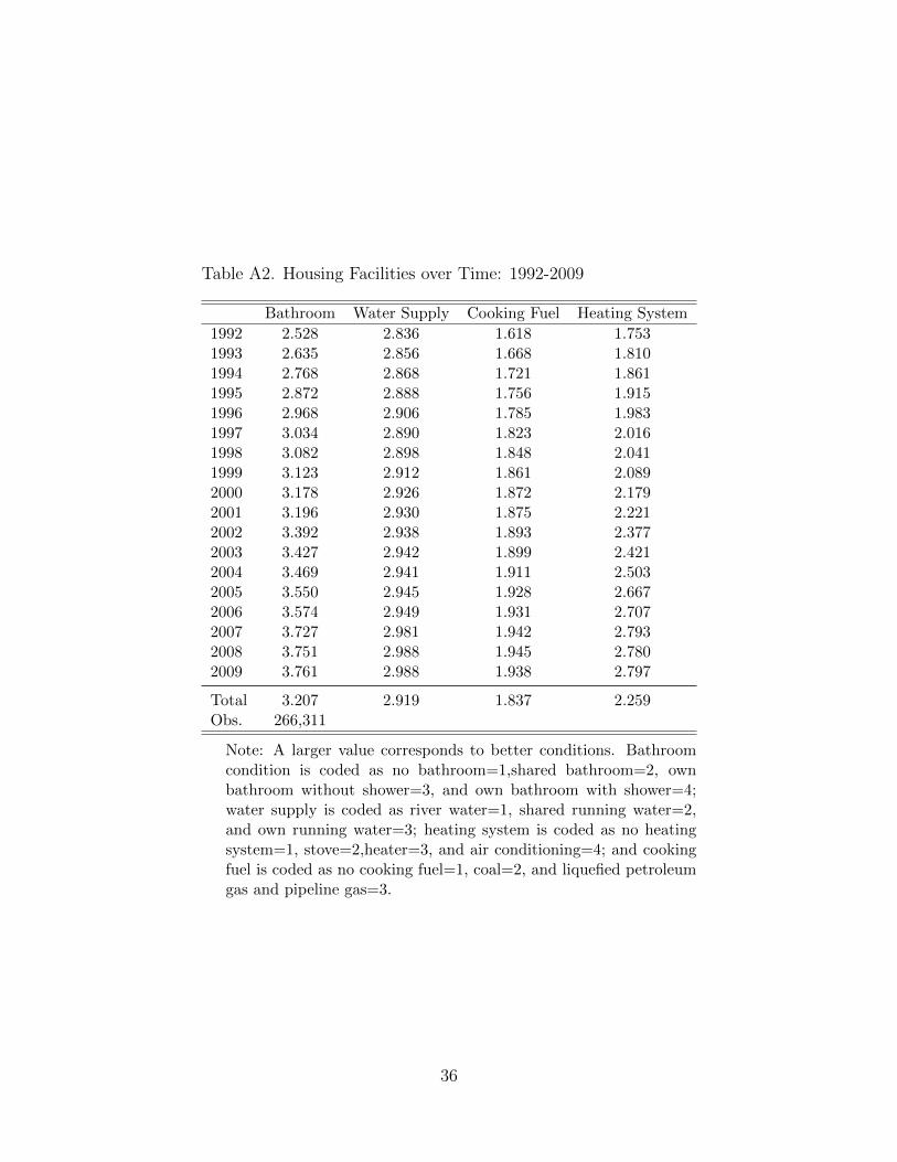
Table A2. Housing Facilities over Time: 1992-2009

Bathroom Water Supply Cooking Fuel Heating System

1992 2.528 2.836 1.618 1.7531993 2.635 2.856 1.668 1.8101994 2.768 2.868 1.721 1.8611995 2.872 2.888 1.756 1.9151996 2.968 2.906 1.785 1.9831997 3.034 2.890 1.823 2.0161998 3.082 2.898 1.848 2.0411999 3.123 2.912 1.861 2.0892000 3.178 2.926 1.872 2.1792001 3.196 2.930 1.875 2.2212002 3.392 2.938 1.893 2.3772003 3.427 2.942 1.899 2.4212004 3.469 2.941 1.911 2.5032005 3.550 2.945 1.928 2.6672006 3.574 2.949 1.931 2.7072007 3.727 2.981 1.942 2.7932008 3.751 2.988 1.945 2.7802009 3.761 2.988 1.938 2.797

Total 3.207 2.919 1.837 2.259Obs. 266,311

Note: A larger value corresponds to better conditions. Bathroomcondition is coded as no bathroom=1,shared bathroom=2, ownbathroom without shower=3, and own bathroom with shower=4;water supply is coded as river water=1, shared running water=2,and own running water=3; heating system is coded as no heatingsystem=1, stove=2,heater=3, and air conditioning=4; and cookingfuel is coded as no cooking fuel=1, coal=2, and liquefied petroleumgas and pipeline gas=3.

36

Table A3: Proportion of Poor-Condition Housing:Alternative Definitions

Definition 1 Definition 2 Definition 3

1992 0.341 0.423 0.4341993 0.293 0.396 0.3911994 0.246 0.363 0.3461995 0.220 0.317 0.3081996 0.193 0.287 0.2701997 0.159 0.270 0.2301998 0.142 0.247 0.2071999 0.130 0.232 0.1912000 0.110 0.213 0.1722001 0.105 0.205 0.162

Total 0.199 0.300 0.277Observations 99,325

Note: Definition 1 defines poor-condition houses as thoselacking at least two of the four essential facilities. Defini-tion 2 defines poor-condition houses as those lacking a pri-vate bathroom. Definition 3 defines poor-condition housesas a collective dormitory.

37

Table A4: The 1998 Reform and Household Saving Rates (1992-2001):Alternative Definitions

State-employed Control Group Private-employed Control Group

Def 2 Def 3 Def 2 Def 3

Post98*Treatment 0.014* 0.017** 0.019*** 0.023***(0.009) (0.009) (0.005) (0.007)

Occupation dummies Yes Yes Yes YesCity dummies Yes Yes Yes YesYear dummies Yes Yes Yes Yes

Observations 76,479 76,479 58,661 58,661R2 0.099 0.117 0.121 0.132

Note: Definition 1 defines poor-condition houses as those lacking at least two of the four essen-tial facilities. Definition 2 defines poor-condition houses as those lacking a private bathroom.Definition 3 defines poor-condition houses as a collective dormitory. Our baseline regressions inTables 5 and 6 use definition 1.

38

A5: The Pace of the 1998 Reform and the SOEReform at the Province Level: 1998-2001

Housing Reform SOE Reform

1997 1998-2001 1997 1998-2001

Beijing 0.88 -0.20 0.47 -0.03Shanxi 0.69 -0.08 0.53 -0.08Liaoning 0.68 -0.37 0.51 -0.06Heilongjiang 0.53 -0.30 0.46 -0.09Jiangsu 0.59 -0.23 0.53 -0.08Zhejiang 0.38 -0.25 0.51 -0.19Anhui 0.62 -0.23 0.56 -0.15Jiangxi 0.71 -0.23 0.56 -0.09Shandong 0.76 -0.40 0.60 -0.09Henan 0.61 -0.10 0.51 -0.10Hubei 0.83 -0.13 0.54 -0.04Guangdong 0.80 -0.52 0.46 -0.06Chongqing 0.76 -0.37 0.58 -0.11Sichuan 0.55 -0.29 0.49 -0.14Yunnan 0.37 -0.19 0.57 -0.08Shaanxi 0.84 -0.00 0.50 -0.09Gansu 0.81 -0.25 0.49 -0.04Total 0.67 -0.24 0.51 -0.09

Note: The pace of the 1998 reform is measured bythe decrease in the proportion of public housingamong urban households from 1998 to 2001. Thepace of the SOE reform is measured by the decreasein the proportion of SOE employees among all ur-ban workers from 1998 to 2001.

39