Household Economic Inequality in Australia · Household Economic Inequality in Australia Rosetta...

Research Discussion Paper

Household Economic Inequality in Australia

Rosetta Dollman, Greg Kaplan, Gianni La Cava and Tahlee Stone

RDP 2015-15

Figures in this publication were generated using Mathematica.

The contents of this publication shall not be reproduced, sold or distributed without the prior consent of the Reserve Bank of Australia and, where applicable, the prior consent of the external source concerned. Requests for consent should be sent to the Head of Information Department at the email address shown above.

ISSN 1448-5109 (Online)

The Discussion Paper series is intended to make the results of the current economic research within the Reserve Bank available to other economists. Its aim is to present preliminary results of research so as to encourage discussion and comment. Views expressed in this paper are those of the authors and not necessarily those of the Reserve Bank. Use of any results from this paper should clearly attribute the work to the authors and not to the Reserve Bank of Australia.

Enquiries:

Phone: +61 2 9551 9830 Facsimile: +61 2 9551 8033 Email: [email protected] Website: http://www.rba.gov.au



Research Discussion Paper2015-15

December 2015

Economic GroupReserve Bank of Australia

We would like to thank Laura Berger-Thomson, Michael Plumb, John Simon,Peter Tulip and Roger Wilkins for useful comments and suggestions. The viewsexpressed in this paper are our own and do not necessarily reflect those of theReserve Bank of Australia. We are solely responsible for any errors.

Authors: dollmanr, lacavag and stonet at domain rba.gov.au

Media Office: [email protected]

Abstract

We document some new stylised facts about consumption and income inequality(or ‘economic inequality’) among households in Australia. Based on household-level information from the Household Expenditure Survey we find thatconsumption inequality is lower on average than income inequality, but thatincome and consumption inequality have both increased a little since the early1990s, with income inequality increasing by more. These findings are broadlysimilar to the changes in income and consumption inequality documented in otherdeveloped economies.

We provide insight into the welfare implications of these changes using paneldata from the Household, Income and Labour Dynamics in Australia Survey. Wedecompose the broad trends in income inequality into four statistical components:(i) changes in observed household characteristics; (ii) changes in the returns tounobserved skills; (iii) changes in the size of persistent income shocks (reflectingevents such as promotions and long-term unemployment); and (iv) changes in thesize of transitory income shocks (reflecting events such as bonuses, short-termunemployment and short-term illness).

The reported trends in income inequality do not appear to be due to changes inobserved household characteristics, but rather to changes in the size of persistentand transitory income shocks. Since the middle of the 2000s, at least some ofthe increase in income inequality has been due to persistent factors, a conclusionthat is consistent with the rise in consumption inequality over the correspondingperiod.

JEL Classification Numbers: D6, D12, D31, E21, H31Keywords: inequality, income, consumption, imputed rent

i

Table of Contents

1. Introduction 1

2. Definitions of Household Consumption and Income 4

2.1 Data 4

2.2 Imputing Housing Expenditure and Income 5

3. Stylised Facts About Household Economic Inequality 8

3.1 Long-run Trends in Consumption and Income Inequality 8

3.2 Wealth Inequality 13

3.3 Housing Prices, Imputed Rent and Inequality Estimates 16

3.4 Consumption Inequality by Type of Household 19

4. Cross-country Comparisons of Income and Consumption Inequality 20

5. Transitory and Persistent Income Inequality 24

5.1 Error Components Model 27

5.2 Income Mobility 29

6. Conclusion 32

Appendix A: Imputed Rent and the Distributions of Household Expenditureand Income 34

Appendix B: Alternative Survey Measures of Inequality 36

Appendix C: Income Inequality Estimates Using Tax Records 40

References 43

Copyright and Disclaimer Notices 47

ii



1. Introduction

Since the early 1990s, real per capita consumption and disposable income inAustralia have both risen by an average of close to 2 per cent annually. However,aggregate trends can mask important changes over time in the distribution ofincome and spending across households.

We explore how the distribution of living standards has evolved over recentdecades by examining trends in household income and consumption inequality(which we will refer to as ‘household economic inequality’). We also explore someshort-run trends in wealth inequality.

Most of the empirical research to date, particularly for Australia, has focused oninequality in current income. But current income is not necessarily a good guideto welfare. Since most individuals experience a period of growing income duringtheir early working years, and a period of lower income as they transition toretirement, and since individuals can borrow and save to smooth out temporaryfluctuations in income, overall living standards depend more on lifetime incomethan on current income. To gauge inequality in living standards, it is better to focuson that part of household income which is due to factors that are likely to persistthrough time, since this persistent component of income (reflecting things likepromotions and long-term unemployment) is likely to be more strongly correlatedwith lifetime income than the transitory component of income (reflecting thingslike bonuses, short-term illness and temporary lay-offs).

These underlying factors are not easily observed in available datasets. We thus taketwo indirect approaches to estimate the degree of inequality in the persistent (andhence welfare-relevant) component of income for Australia. First, we follow otherstudies that suggest that consumption is a more appropriate measure of household

2

wellbeing than current income or wealth (see, for example, Slesnick (1998)).1

Under this approach, we use repeated cross-sections of the Australian Bureauof Statistics (ABS) Household Expenditure Survey (HES) to examine howconsumption inequality has evolved, relative to inequality in current income andwealth, over recent decades. We also explore some of the drivers of these changesover time.

Our second approach to estimating persistent income inequality is to exploit thepanel dimension of the Melbourne Institute’s Household, Income and LabourDynamics in Australia (HILDA) Survey. By tracking the same households acrosstime we are able to estimate a statistical model of household income dynamics thatallows the distribution of temporary and persistent income to evolve separatelyover time. Through the lens of the estimated model, we can then measure theevolution of each type of inequality.

Our paper is motivated by the recent shift in focus in macroeconomics from thetime series dynamics of household consumption and income to an explorationof the cross-sectional distributions of these variables across households and howthe distributions change over time. Research into the distributions of householdincome and spending is an important input into identifying emerging risks tofinancial stability. It can also broaden our understanding of how monetary andfiscal policies affect the economy. The sensitivity (or resilience) of the householdsector to shocks can be affected by which households are saving and which areborrowing at a given time. For example, aggregate spending will be particularlysensitive to changes in interest rates if there is a relatively large share ofhouseholds that are constrained from borrowing.

Australian research on inequality has increased of late. For instance, Fletcherand Guttmann (2013), Greenville, Pobke and Rogers (2013) and Wilkins (2015)document trends in current income inequality in Australia using household surveydata. They find that there has been a slight increase in income inequality overrecent years which has largely been driven by an increase in capital income atthe top of the distribution. Some Australian studies have also examined trends

1 As consumption is a choice variable, it is more closely connected with the lifetime wealthconstraint faced by households than is current income. If some households smooth temporaryfluctuations in income by borrowing and saving, then income will tend to be more variablethan consumption at a point in time and hence income will overstate the level of inequality inhousehold welfare.

3

in expenditure inequality (e.g. Harding and Greenwell 2002; Bray 2014) andnon-durable consumption inequality (Barrett, Crossley and Worswick 1999).Bray (2014) finds that expenditure inequality has been lower and more stable thanincome inequality over the past three decades, although it appears to have beenincreasing since the late 1990s.

We construct estimates of household economic inequality using several sourcesof data. Our consumption inequality estimates primarily come from the HES.Nevertheless, we explore measures of inequality using other data sources,including the HILDA Survey, the ABS Survey of Income and Housing (SIH) anddata based on individual income tax records provided by the Australian TaxationOffice (ATO).

We will consider a wide range of inequality measures, including indicators thatare specifically designed to measure inequality, such as the Gini coefficient, alongwith simpler measures that are advocated in Piketty (2014), such as the share oftotal household income held by the highest-earning households and the varianceof the logarithm of income. Our paper makes the following contributions:

1. To the best of our knowledge, we are the first to quantify the extent to whichthe trends in income inequality in Australia are due to changes in observablecharacteristics and to changes in the distribution of unobserved persistent andtemporary income shocks.2

2. We construct estimates of consumption inequality that are broader thanprevious Australian studies.

3. We examine in detail how housing prices can affect estimates of householdeconomic inequality. In particular, we show how it can have different effectson estimates of wealth inequality as compared with income and consumptioninequality.

2 We focus on trends in inequality for household income in this paper in order to allow for directcomparisons with the consumption trends, which are only available at a household level. Wehave also examined the trends in individual income inequality, but the key results are basicallythe same.

4

Our key findings are that:

1. Consumption inequality is lower on average than income inequality and hasrisen by less since at least the early 1990s.

2. The rise in consumption inequality has reflected a relatively large increase inspending by the highest-spending households (within the top 1 per cent of thedistribution).

3. The increase in income inequality over the past decade has not been dueto observable factors, such as an ageing population or rising educationalattainment. Instead, it has reflected an increase in the variance of unobservedshocks, particularly since the middle of the 2000s. At least some of theincrease in income inequality has been persistent, implying higher inequalityin household welfare.

2. Definitions of Household Consumption and Income

2.1 Data

The analysis in this paper is primarily based on unit record data from the HESfor six different surveys: 1984, 1988/89, 1993/94, 1998/99, 2003/04 and 2009/10.The HES is the most comprehensive source of cross-sectional informationon household expenditure in Australia.3 For comparability with the spendingestimates, we focus on the HES estimates of income. To examine the driversof inequality we also examine measures based on the HILDA Survey. In theAppendices, we provide alternative estimates of inequality using tax records.

It is not straightforward to use the HES to derive a long time series of eitherexpenditure or income. A key obstacle to making time series comparisons ofincome inequality is that the ABS has developed more sophisticated ways tomeasure income over time. For example, in 2003/04, the ABS incorporatedinformation on salary sacrificed income into their household income estimatesfor the first time. This is likely to have boosted measured inequality relative

3 The HILDA Survey also collects annual estimates of expenditure. However, the expendituredefinitions have changed over time and are not as complete as the HES.

5

to earlier surveys as high-income earners are more likely to engage in salarysacrificing. Despite this, in each HES, the ABS provides estimates of income basedon definitions from earlier surveys. This helps us match the income measures overtime to generate a reasonably comparable time series. Moreover, we have foundthat the income definitions can affect the estimated level of inequality in any givensurvey, but the broad trends in measured inequality are similar regardless of thedefinition of income.4

In this paper we examine inequality in both gross and disposable householdincome. This allows us to examine the role of government taxes and transfersin affecting inequality. We follow the ABS in defining disposable income as grossincome after deducting personal income tax and the Medicare levy. In additionto changes in the definitions of income, the ABS also changed the way it collectshousehold-level tax data. Prior to the late 1980s, the tax data are calculated using acombination of actual reported taxes and imputations, but the tax data for the latersurveys are entirely imputed, which is now the preferred method of the ABS forestimating taxes in household surveys. This complicates comparisons of inequalityin disposable income before and after the early 1990s (Barrett et al 1999). Partlyfor this reason, we mainly focus our analysis on the period since the early 1990s.

2.2 Imputing Housing Expenditure and Income

To construct our preferred estimates of household consumption and income weadjust the raw data. Most importantly, we add a service-flow equivalent of housingexpenditure for owner-occupiers (or ‘net imputed rent’) to both the consumptionand income estimates. Imputed rent is the value of housing services that owner-occupiers receive from living in a rent-free dwelling and it constitutes a significantcomponent of non-cash household income and consumption.

Most guidelines for the compilation of income distribution statistics recommendthe inclusion of imputed rent in both consumption and income. Conceptually, theinclusion of imputed rent as part of income treats owner-occupiers as if they wererenting the home from themselves, so they are simultaneously paying rent and

4 Despite these caveats, the ABS publishes its own time series of income inequality estimatesbased on the SIH. The trends in the SIH estimates broadly align with those identified in thispaper. Wilkins (2013) provides a very detailed discussion of the relative merits of the inequalityestimates obtained from the various data sources.

6

earning rental income (Saunders and Siminski 2005). The imputed rent adjustmentessentially makes estimates of consumption and income for renters comparable tothose of owner-occupiers. Doing otherwise can lead to unintuitive results.

To see this, consider the following example. Persons A and B live next door toeach other in identical homes. They are the same in all respects; they pay thesame amount of rent, spend the same amount on other goods and services, andthey have the same income and wealth. Suppose that person A decides to buythe home they currently rent by running down their savings in a bank deposit.In contrast, person B continues to rent. Without any imputed rent adjustment,person A’s measured expenditure falls relative to person B because they no longerpay rent. And their measured income also falls relative to person B because theylose the interest earnings on their deposit account. In a sense, without adjusting forimputed rent, person A would appear ‘worse off’ than person B simply becausethey became a home owner.

In contrast, with an imputed rent adjustment, person A’s consumption isunchanged as, under reasonable assumptions, the rent that is imputed is the sameas the existing market rent. Their income is also unchanged to the extent that theimputed rent is the same as the interest they previously earned on their savingsaccount.5 In other words, with the adjustment for imputed rent, persons A andB are still basically in the same welfare position as before, despite person Abecoming a home owner.6

Net imputed rent is equal to the estimated market rent of a dwelling (‘grossimputed rent’) less housing costs normally paid by a landlord such as mortgageinterest, rates, insurance and repairs. Total household ‘consumption’ is then equal

5 This requires some ‘hand waving’, as standard theory would suggest the returns on the homeand the bank deposit need not be the same every period but only over the lives of the two assets.

6 Similar logic applies if person A borrows the full amount to buy the home rather thanselling an existing asset. For simplicity, assume it is an interest-only mortgage loan. Withoutthe imputed rent adjustment, person A’s measured expenditure falls relative to person Bbecause the home owner pays interest rather than rent, and interest payments are not part ofconsumption. Person A’s measured income also falls as interest payments are deducted fromincome (otherwise interest earnings and interest payments are treated differently). With theimputed rent adjustment, person A’s consumption is unchanged by the home ownership decision(as before). And their income is unchanged to the extent that the imputed rent is equal to theinterest paid on the loan. If the imputed rent is larger (smaller) than the interest paid thenperson A’s income rises (falls) relative to person B.

7

to total household ‘expenditure’ on goods and services plus net imputed rent.Similarly, ‘adjusted’ income is equal to reported income plus net imputed rent.In Appendix A, we provide a more detailed description of the differences betweenhousehold consumption and expenditure.

The gross imputed rent estimates are based on the self-reported value of eachowner-occupier’s dwelling; weekly gross imputed rent is defined to be equal to5 per cent of the self-reported value of the owner-occupier’s dwelling (dividedby 52 weeks). The choice of 5 per cent for the ‘imputed rental yield’ is basedon previous Australian research (Yates 1994; Saunders and Siminski 2005). Thebenefit of this approach to estimating imputed rent is that it is straightforward toimplement and it fully utilises the available self-reported data on dwelling values.As the ABS has only made information on the reported dwelling value publiclyavailable from 1993/94 onwards, we concentrate on the most recent four surveys:1993/94, 1998/99, 2003/04 and 2009/10.

In Appendix B, we provide estimates of inequality using an alternative measure ofimputed rent based on a hedonic modelling framework. This modelling approachestimates the market value of the rental equivalent for owner-occupied dwellingsusing information on comparable rented dwellings. This alternative approachallows the implied rental yield to vary over time. A comparison of the twoapproaches highlights the fact that measures of inequality are somewhat sensitiveto the treatment of housing income and expenditure. Nevertheless, the generaltrends in household economic inequality are fairly similar under this alternativeapproach. We find that consumption and income inequality have increased sincethe early 1990s using either the baseline or alternative approach to estimatingimputed rent. For a more detailed discussion of the inequality estimates using thisalternative approach, see Beech et al (2014).

Our estimates of consumption deduct both mortgage interest payments and interestpayments on other forms of debt (e.g. personal loans and credit cards) fromtotal expenditure. Interest payments do not represent a flow of services to thehousehold. All income and consumption estimates are population weighted anddivided by an equivalence factor to control for household size and composition.7

7 The estimated trends in inequality presented in this paper are largely unaffected by the use ofan equivalence factor.

8

There are some caveats to our consumption estimates. First, consumption is abetter guide to living standards than current income, but it is still not a completemeasure of household wellbeing. Most notably, our estimates do not includemeasures of consumption of public goods (e.g. recreational facilities), socialtransfers in kind (e.g. government-funded goods and services such as publichealth care and education), or goods that are produced within the home. Datalimitations prevent us from constructing these broader estimates of consumption.By excluding items such as social transfers in kind, we will tend to overstate thelevel of economic inequality (Barrett et al 1999).8 But it is less clear whether theexclusion of these items affects the estimated trends in inequality. Second, we donot convert all durable goods expenditure to a service-flow equivalent because wedo not have long-run household-level data on the stock of such durable goods.However, we have found that excluding spending on particular durable goods,such as motor vehicles, has little discernible effect on our inequality estimates.9

Third, we also do not examine trends in the distribution of leisure time, which isanother indicator of household wellbeing (Attanasio, Hurst and Pistaferri 2014).

3. Stylised Facts About Household Economic Inequality

3.1 Long-run Trends in Consumption and Income Inequality

There are several different indicators of inequality that are typically used in theliterature. The most common measure of inequality is the Gini coefficient, which isderived from the Lorenz curve. The Lorenz curve shows the share of spending (orincome) by households ranked by spending (or income). The further the curve isbelow the 45 degree line, the less equal the distribution. Correspondingly, the Ginicoefficient is calculated as the area between the Lorenz curve and the 45 degreeline divided by the total area under the 45 degree line. The Gini coefficientranges from zero to one, where zero represents perfect equality and one representscomplete inequality.

8 The most recent HES for 2009/10 provides estimates of social transfers in kind. The inclusionof such transfers reduces disposable income inequality by about one-quarter, on average.

9 The 2003/04 and 2009/10 HES provide information on the total (net) value of the stock ofvehicles owned by households. Replacing the reported expenditure on motor vehicles with theservice-flow equivalent (measured as 10 per cent of the net value of the stock of vehicles)slightly reduces the estimates of expenditure inequality for the two survey years, and leads to alarger increase in measured inequality between the two periods.

9

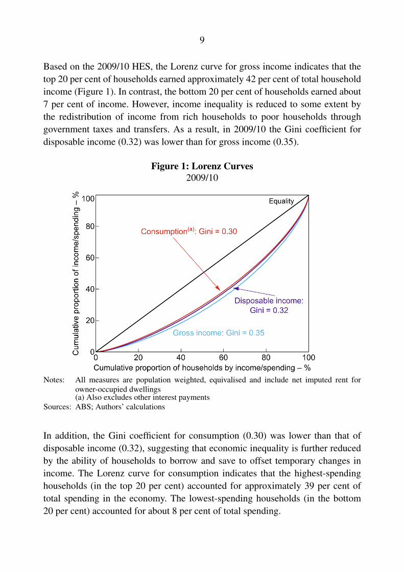
Based on the 2009/10 HES, the Lorenz curve for gross income indicates that thetop 20 per cent of households earned approximately 42 per cent of total householdincome (Figure 1). In contrast, the bottom 20 per cent of households earned about7 per cent of income. However, income inequality is reduced to some extent bythe redistribution of income from rich households to poor households throughgovernment taxes and transfers. As a result, in 2009/10 the Gini coefficient fordisposable income (0.32) was lower than for gross income (0.35).

Figure 1: Lorenz Curves2009/10

Notes: All measures are population weighted, equivalised and include net imputed rent forowner-occupied dwellings(a) Also excludes other interest payments

Sources: ABS; Authors’ calculations

In addition, the Gini coefficient for consumption (0.30) was lower than that ofdisposable income (0.32), suggesting that economic inequality is further reducedby the ability of households to borrow and save to offset temporary changes inincome. The Lorenz curve for consumption indicates that the highest-spendinghouseholds (in the top 20 per cent) accounted for approximately 39 per cent oftotal spending in the economy. The lowest-spending households (in the bottom20 per cent) accounted for about 8 per cent of total spending.

10

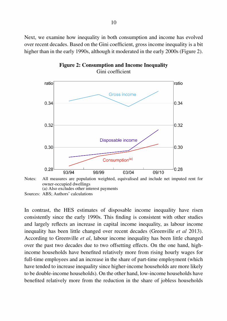
Next, we examine how inequality in both consumption and income has evolvedover recent decades. Based on the Gini coefficient, gross income inequality is a bithigher than in the early 1990s, although it moderated in the early 2000s (Figure 2).

Figure 2: Consumption and Income InequalityGini coefficient



In contrast, the HES estimates of disposable income inequality have risenconsistently since the early 1990s. This finding is consistent with other studiesand largely reflects an increase in capital income inequality, as labour incomeinequality has been little changed over recent decades (Greenville et al 2013).According to Greenville et al, labour income inequality has been little changedover the past two decades due to two offsetting effects. On the one hand, high-income households have benefited relatively more from rising hourly wages forfull-time employees and an increase in the share of part-time employment (whichhave tended to increase inequality since higher-income households are more likelyto be double-income households). On the other hand, low-income households havebenefited relatively more from the reduction in the share of jobless households

11

(which has tended to reduce inequality), which is consistent with the substantialtrend decline in the unemployment rate since the early 1990s.

Consumption inequality has been consistently lower than both gross anddisposable income inequality. Furthermore, the increase in consumption inequalityhas also been less pronounced than the increase in disposable income inequalitysince the early 1990s. In Section 4 we show that these trends have also beenobserved in other advanced economies. We explore drivers of these changes inthe next section of the paper.

The Gini coefficient is a useful indicator for summarising distributions. However,it does not identify which parts of the distribution are responsible for anychanges over time. It is also not a particularly intuitive measure of inequality. Tocomplement the analysis, we examine how much of aggregate household incomeis earned by the high-income households (as a proxy for income inequality) and,similarly, how much of aggregate household consumption is accounted for by thehigh-spending households (for consumption inequality).

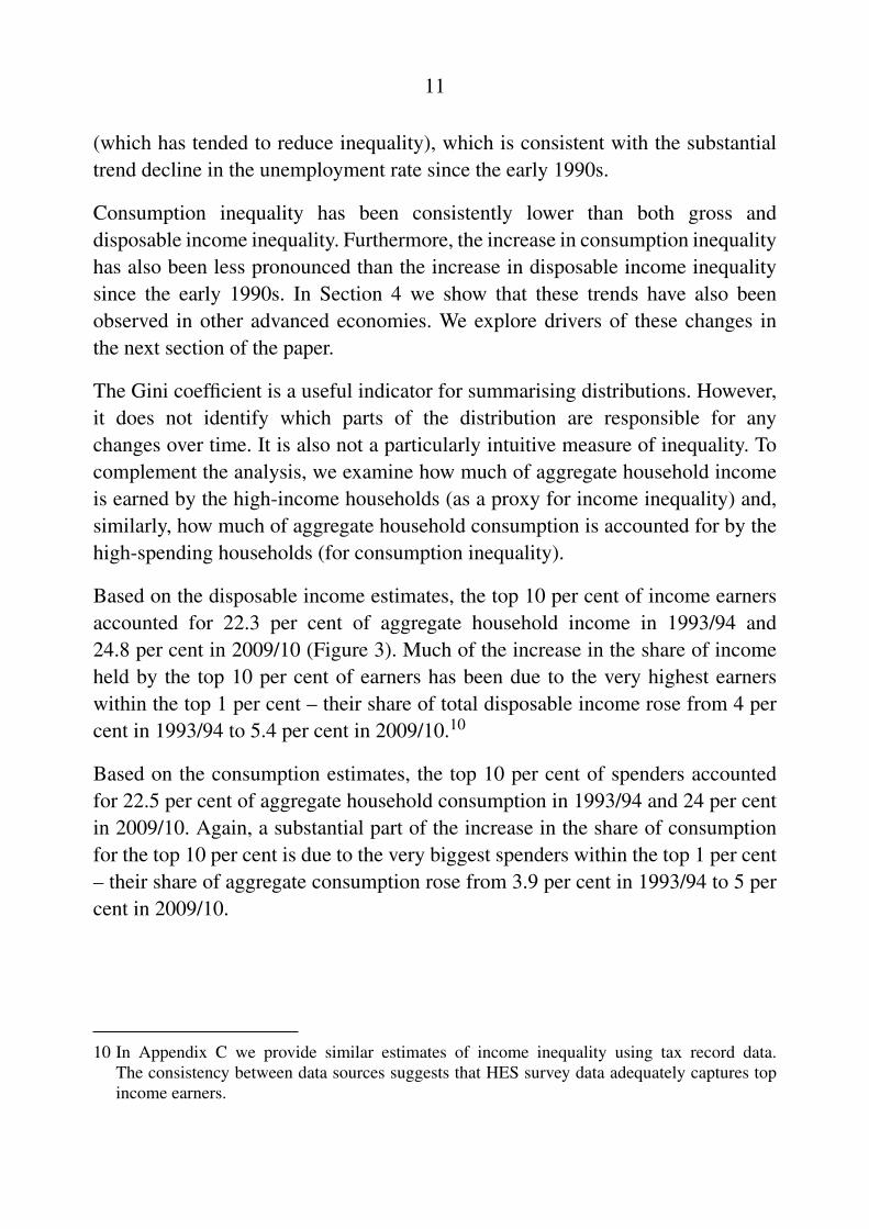
Based on the disposable income estimates, the top 10 per cent of income earnersaccounted for 22.3 per cent of aggregate household income in 1993/94 and24.8 per cent in 2009/10 (Figure 3). Much of the increase in the share of incomeheld by the top 10 per cent of earners has been due to the very highest earnerswithin the top 1 per cent – their share of total disposable income rose from 4 percent in 1993/94 to 5.4 per cent in 2009/10.10

Based on the consumption estimates, the top 10 per cent of spenders accountedfor 22.5 per cent of aggregate household consumption in 1993/94 and 24 per centin 2009/10. Again, a substantial part of the increase in the share of consumptionfor the top 10 per cent is due to the very biggest spenders within the top 1 per cent– their share of aggregate consumption rose from 3.9 per cent in 1993/94 to 5 percent in 2009/10.

10 In Appendix C we provide similar estimates of income inequality using tax record data.The consistency between data sources suggests that HES survey data adequately captures topincome earners.

12

Figure 3: Top Income Earners/ConsumersShare of total household income/consumption



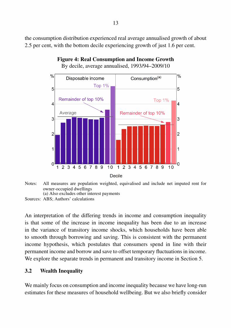
To further examine different parts of the income and consumption distributions,we break down each distribution into deciles and separate out the top 1 per cent.We then examine the relative growth in income and consumption for each decileand the top 1 per cent. Based on this, the top 1 per cent of earners experienceda relatively large increase in real disposable income of just over 5 per cent perannum between 1993/94 and 2009/10 (Figure 4). In contrast, the bottom 99 percent of households experienced real annualised income growth of about 3 percent, with the bottom decile experiencing much lower growth than the rest ofthe distribution. The top 1 per cent of spenders have also experienced fastergrowth in real consumption than other households over recent decades, though thedifference in growth is less pronounced than in the case of income (Figure 4). Morespecifically, the top 1 per cent of spenders experienced real growth in consumptionof a bit over 4 per cent. In contrast, households in the bottom 99 per cent of

13

the consumption distribution experienced real average annualised growth of about2.5 per cent, with the bottom decile experiencing growth of just 1.6 per cent.

Figure 4: Real Consumption and Income GrowthBy decile, average annualised, 1993/94–2009/10



An interpretation of the differing trends in income and consumption inequalityis that some of the increase in income inequality has been due to an increasein the variance of transitory income shocks, which households have been ableto smooth through borrowing and saving. This is consistent with the permanentincome hypothesis, which postulates that consumers spend in line with theirpermanent income and borrow and save to offset temporary fluctuations in income.We explore the separate trends in permanent and transitory income in Section 5.

3.2 Wealth Inequality

We mainly focus on consumption and income inequality because we have long-runestimates for these measures of household wellbeing. But we also briefly consider

14

wealth inequality for two reasons. First, wealth is a potentially important indicatorof wellbeing in its own right. Second, it highlights the important role of housingprices in affecting measured inequality. To develop the most complete picture weconsider estimates of wealth inequality from both the HES and SIH.

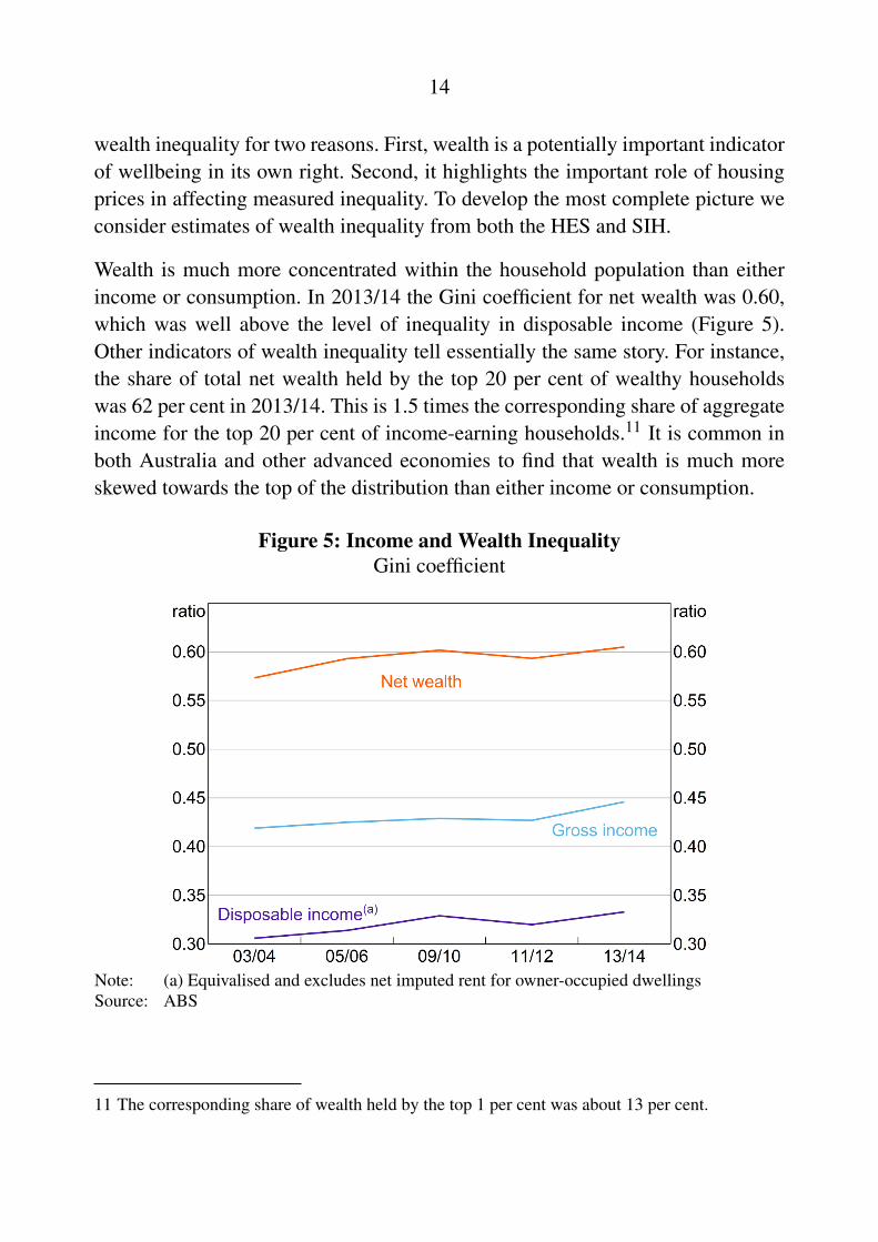
Wealth is much more concentrated within the household population than eitherincome or consumption. In 2013/14 the Gini coefficient for net wealth was 0.60,which was well above the level of inequality in disposable income (Figure 5).Other indicators of wealth inequality tell essentially the same story. For instance,the share of total net wealth held by the top 20 per cent of wealthy householdswas 62 per cent in 2013/14. This is 1.5 times the corresponding share of aggregateincome for the top 20 per cent of income-earning households.11 It is common inboth Australia and other advanced economies to find that wealth is much moreskewed towards the top of the distribution than either income or consumption.

Figure 5: Income and Wealth InequalityGini coefficient

Note: (a) Equivalised and excludes net imputed rent for owner-occupied dwellingsSource: ABS

11 The corresponding share of wealth held by the top 1 per cent was about 13 per cent.

15

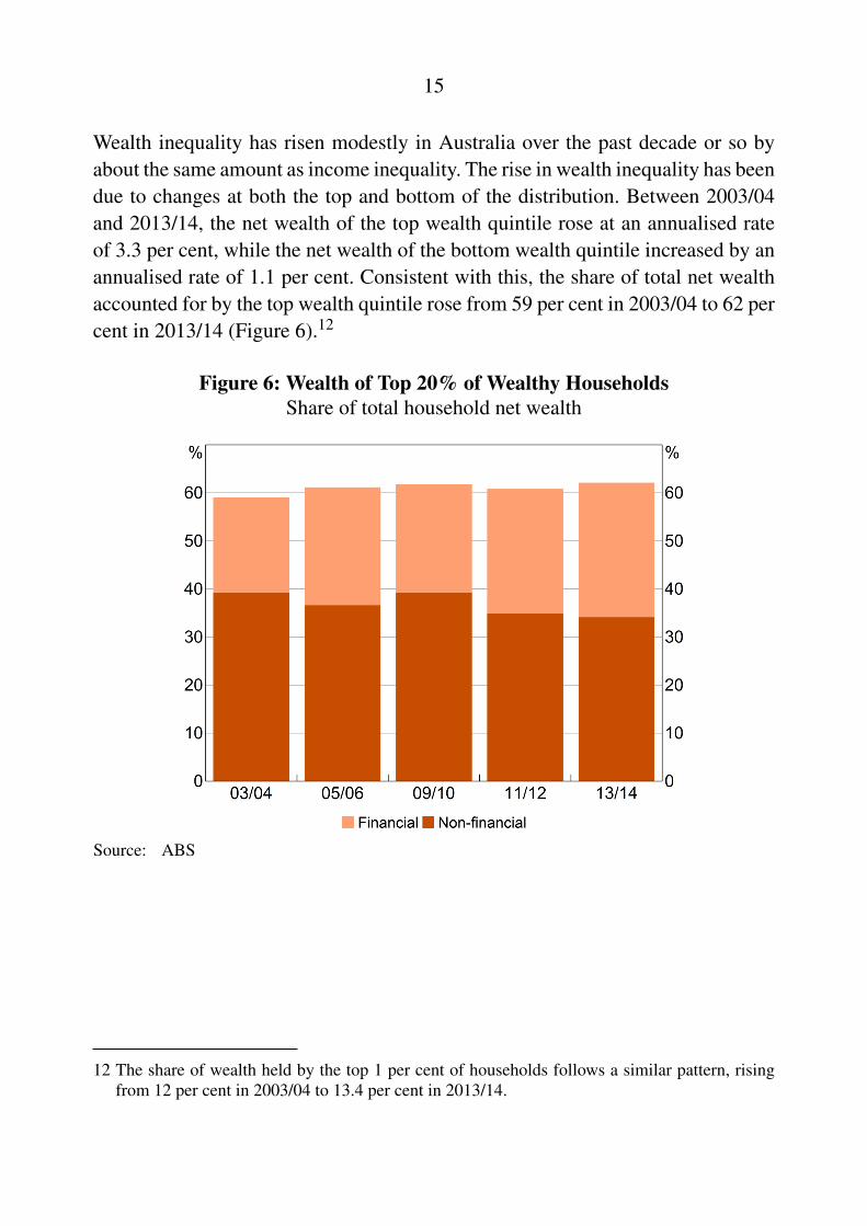
Wealth inequality has risen modestly in Australia over the past decade or so byabout the same amount as income inequality. The rise in wealth inequality has beendue to changes at both the top and bottom of the distribution. Between 2003/04and 2013/14, the net wealth of the top wealth quintile rose at an annualised rateof 3.3 per cent, while the net wealth of the bottom wealth quintile increased by anannualised rate of 1.1 per cent. Consistent with this, the share of total net wealthaccounted for by the top wealth quintile rose from 59 per cent in 2003/04 to 62 percent in 2013/14 (Figure 6).12

Figure 6: Wealth of Top 20% of Wealthy HouseholdsShare of total household net wealth

Source: ABS

12 The share of wealth held by the top 1 per cent of households follows a similar pattern, risingfrom 12 per cent in 2003/04 to 13.4 per cent in 2013/14.

16

As in most advanced economies, housing wealth is the largest component ofaggregate household wealth in Australia. Somewhat surprisingly though, changesin housing prices have not been the main determinants of changes in wealthinequality over the past decade. Instead, the rise in wealth inequality has been dueto a rise in inequality in financial wealth and, in particular, an increase in the valueof holdings of private superannuation and debt instruments (such as debenturesand bonds) for the wealthiest households.

3.3 Housing Prices, Imputed Rent and Inequality Estimates

The estimates of household consumption and income inequality presented in theprevious section include a service-flow equivalent of housing expenditure forowner-occupiers (or ‘net imputed rent’). It is worth discussing the adjustment fornet imputed rent in detail as it has a significant effect on estimates of both the leveland cross-sectional distribution of consumption and income in the economy.

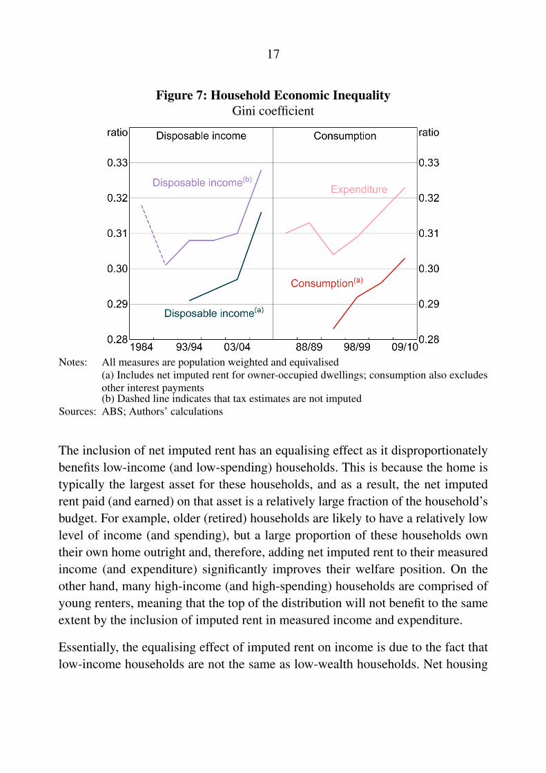
The household surveys show that the inclusion of net imputed rent significantlyreduces the level of inequality in both income and spending. Based on theGini coefficient, the addition of net imputed rent reduces measured inequalityin spending by a bit over 6 per cent, on average. This is shown by the fact thattotal consumption is more equally distributed across households than goods andservices expenditure, on average (Figure 7). (Recall that household ‘consumption’is the sum of household ‘expenditure’ and net imputed rent.) Similarly, theaddition of net imputed rent reduces inequality in disposable income by just under5 per cent on average.

17

Figure 7: Household Economic InequalityGini coefficient

Notes: All measures are population weighted and equivalised(a) Includes net imputed rent for owner-occupied dwellings; consumption also excludesother interest payments(b) Dashed line indicates that tax estimates are not imputed


The inclusion of net imputed rent has an equalising effect as it disproportionatelybenefits low-income (and low-spending) households. This is because the home istypically the largest asset for these households, and as a result, the net imputedrent paid (and earned) on that asset is a relatively large fraction of the household’sbudget. For example, older (retired) households are likely to have a relatively lowlevel of income (and spending), but a large proportion of these households owntheir own home outright and, therefore, adding net imputed rent to their measuredincome (and expenditure) significantly improves their welfare position. On theother hand, many high-income (and high-spending) households are comprised ofyoung renters, meaning that the top of the distribution will not benefit to the sameextent by the inclusion of imputed rent in measured income and expenditure.

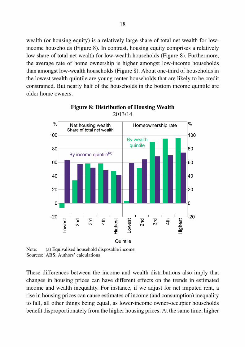
Essentially, the equalising effect of imputed rent on income is due to the fact thatlow-income households are not the same as low-wealth households. Net housing

18

wealth (or housing equity) is a relatively large share of total net wealth for low-income households (Figure 8). In contrast, housing equity comprises a relativelylow share of total net wealth for low-wealth households (Figure 8). Furthermore,the average rate of home ownership is higher amongst low-income householdsthan amongst low-wealth households (Figure 8). About one-third of households inthe lowest wealth quintile are young renter households that are likely to be creditconstrained. But nearly half of the households in the bottom income quintile areolder home owners.

Figure 8: Distribution of Housing Wealth2013/14

Note: (a) Equivalised household disposable incomeSources: ABS; Authors’ calculations

These differences between the income and wealth distributions also imply thatchanges in housing prices can have different effects on the trends in estimatedincome and wealth inequality. For instance, if we adjust for net imputed rent, arise in housing prices can cause estimates of income (and consumption) inequalityto fall, all other things being equal, as lower-income owner-occupier householdsbenefit disproportionately from the higher housing prices. At the same time, higher

19

housing prices cause estimated wealth inequality to rise as wealthier householdsbenefit disproportionately.

3.4 Consumption Inequality by Type of Household

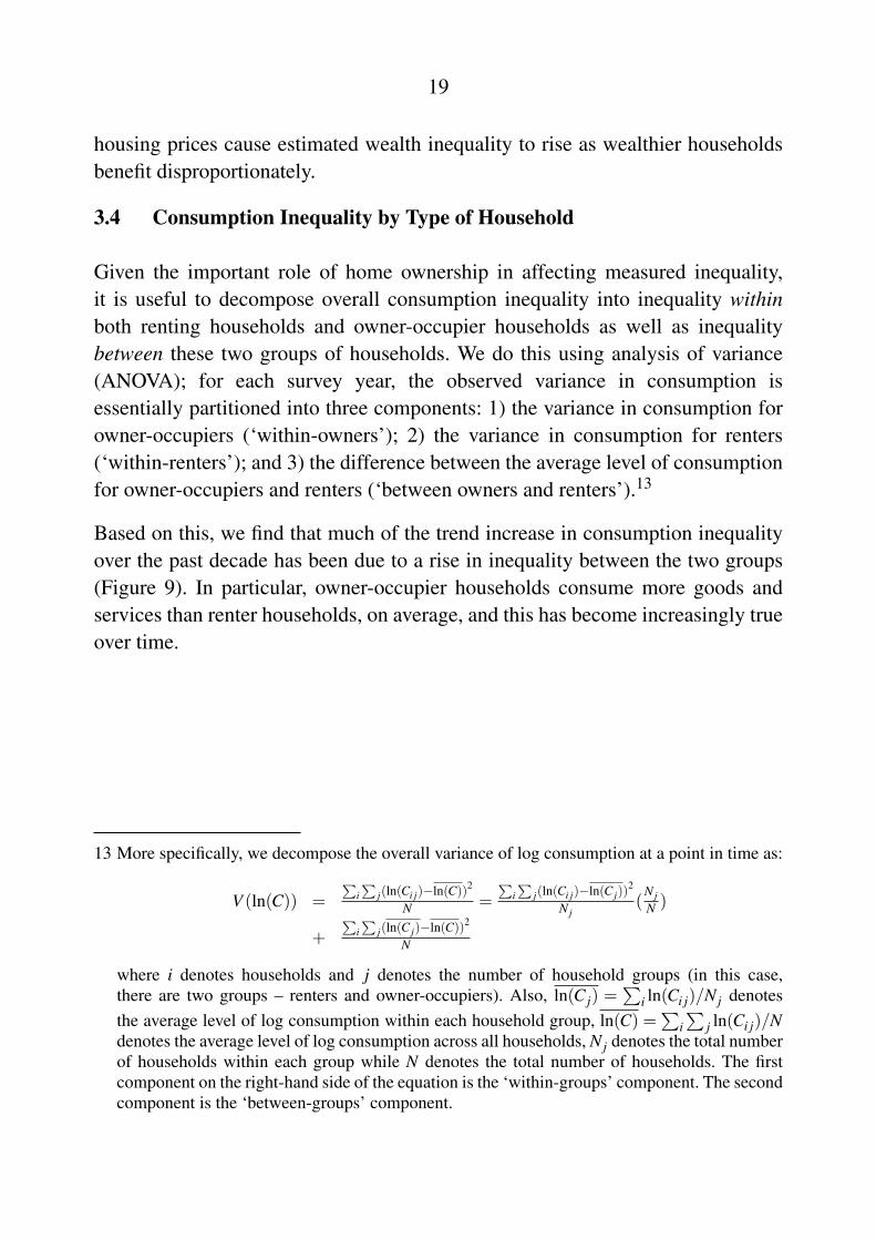
Given the important role of home ownership in affecting measured inequality,it is useful to decompose overall consumption inequality into inequality withinboth renting households and owner-occupier households as well as inequalitybetween these two groups of households. We do this using analysis of variance(ANOVA); for each survey year, the observed variance in consumption isessentially partitioned into three components: 1) the variance in consumption forowner-occupiers (‘within-owners’); 2) the variance in consumption for renters(‘within-renters’); and 3) the difference between the average level of consumptionfor owner-occupiers and renters (‘between owners and renters’).13

Based on this, we find that much of the trend increase in consumption inequalityover the past decade has been due to a rise in inequality between the two groups(Figure 9). In particular, owner-occupier households consume more goods andservices than renter households, on average, and this has become increasingly trueover time.

13 More specifically, we decompose the overall variance of log consumption at a point in time as:

V (ln(C)) =∑

i∑

j(ln(Ci j)−ln(C))2

N =∑

i∑

j(ln(Ci j)−ln(C j))2

N j(

N jN )

+∑

i∑

j(ln(C j)−ln(C))2

N

where i denotes households and j denotes the number of household groups (in this case,there are two groups – renters and owner-occupiers). Also, ln(C j) =

∑i ln(Ci j)/N j denotes

the average level of log consumption within each household group, ln(C) =∑

i∑

j ln(Ci j)/Ndenotes the average level of log consumption across all households, N j denotes the total numberof households within each group while N denotes the total number of households. The firstcomponent on the right-hand side of the equation is the ‘within-groups’ component. The secondcomponent is the ‘between-groups’ component.

20

Figure 9: Decomposition of Consumption Inequality

Notes: Decomposition of the variance of the logarithm of consumption; includes net imputedrent for owner-occupied dwellings and excludes other interest payments

Source: ABS; Authors’ calculations

4. Cross-country Comparisons of Income and ConsumptionInequality

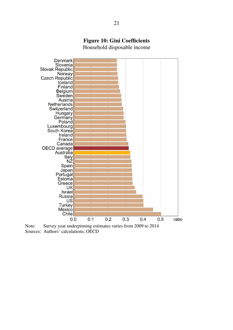
We can compare the inequality estimates for Australia with correspondingestimates in other countries. The Organisation for Economic Co-operation andDevelopment (OECD) has produced estimates of income inequality based on theGini coefficient that allow for comparisons across countries. According to thelatest estimates, the level of inequality in Australia is only slightly higher thanthe OECD average (Figure 10).

21

Figure 10: Gini CoefficientsHousehold disposable income

Note: Survey year underpinning estimates varies from 2009 to 2014Sources: Authors’ calculations; OECD

22

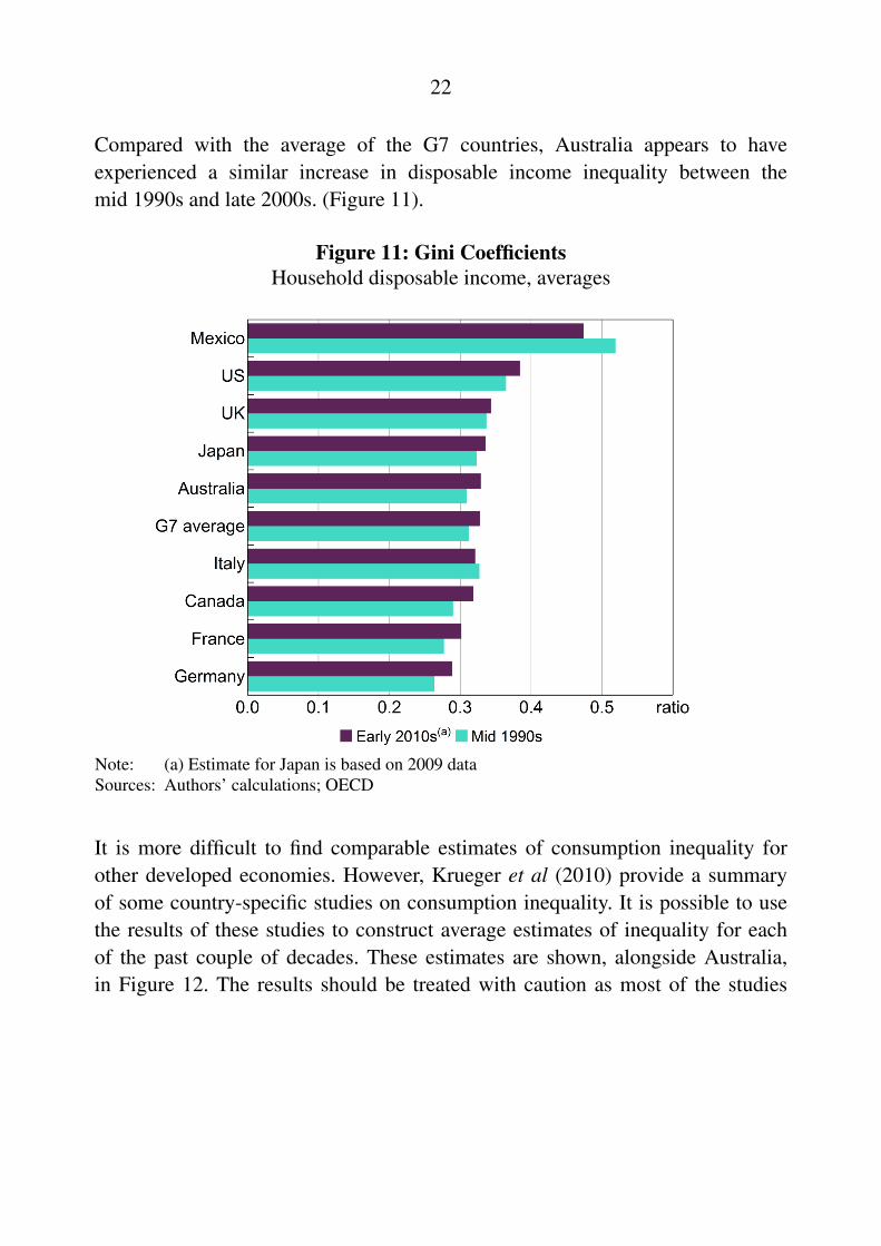
Compared with the average of the G7 countries, Australia appears to haveexperienced a similar increase in disposable income inequality between themid 1990s and late 2000s. (Figure 11).

Figure 11: Gini CoefficientsHousehold disposable income, averages

Note: (a) Estimate for Japan is based on 2009 dataSources: Authors’ calculations; OECD

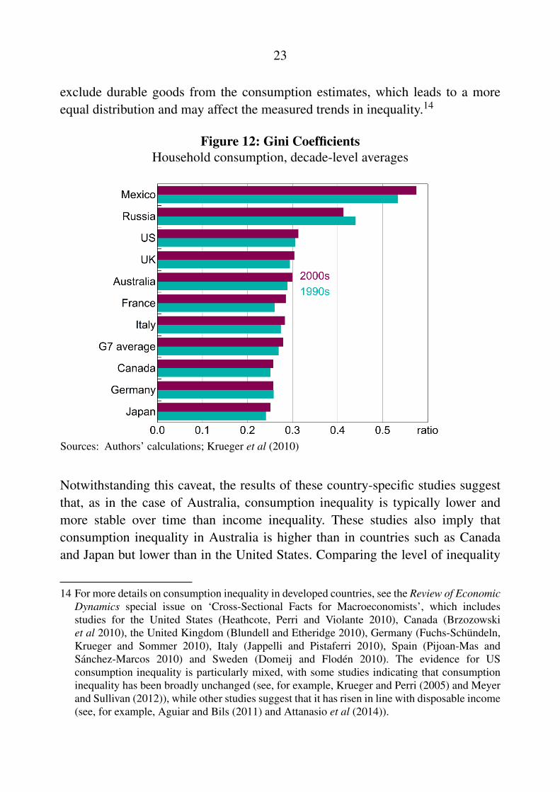
It is more difficult to find comparable estimates of consumption inequality forother developed economies. However, Krueger et al (2010) provide a summaryof some country-specific studies on consumption inequality. It is possible to usethe results of these studies to construct average estimates of inequality for eachof the past couple of decades. These estimates are shown, alongside Australia,in Figure 12. The results should be treated with caution as most of the studies

23

exclude durable goods from the consumption estimates, which leads to a moreequal distribution and may affect the measured trends in inequality.14

Figure 12: Gini CoefficientsHousehold consumption, decade-level averages

Sources: Authors’ calculations; Krueger et al (2010)

Notwithstanding this caveat, the results of these country-specific studies suggestthat, as in the case of Australia, consumption inequality is typically lower andmore stable over time than income inequality. These studies also imply thatconsumption inequality in Australia is higher than in countries such as Canadaand Japan but lower than in the United States. Comparing the level of inequality

14 For more details on consumption inequality in developed countries, see the Review of EconomicDynamics special issue on ‘Cross-Sectional Facts for Macroeconomists’, which includesstudies for the United States (Heathcote, Perri and Violante 2010), Canada (Brzozowskiet al 2010), the United Kingdom (Blundell and Etheridge 2010), Germany (Fuchs-Schundeln,Krueger and Sommer 2010), Italy (Jappelli and Pistaferri 2010), Spain (Pijoan-Mas andSanchez-Marcos 2010) and Sweden (Domeij and Floden 2010). The evidence for USconsumption inequality is particularly mixed, with some studies indicating that consumptioninequality has been broadly unchanged (see, for example, Krueger and Perri (2005) and Meyerand Sullivan (2012)), while other studies suggest that it has risen in line with disposable income(see, for example, Aguiar and Bils (2011) and Attanasio et al (2014)).

24

in the 2000s to that in the 1990s, it appears that Australia experienced a slightincrease in inequality very similar to that of the G7 countries.

5. Transitory and Persistent Income Inequality

According to Friedman’s (1957) permanent income hypothesis, the distributionof household consumption should closely resemble the distribution of permanentincome. So an alternative way to examine how household economic inequality hasevolved, and to understand its welfare implications, is to explore whether changesin income inequality have been driven by persistent or transitory shocks to income.

The distinction between persistent and transitory income can be important for acouple of reasons (outlined in DeBacker et al (2013)). First, the distinction mayhelp to understand the determinants of higher annual cross-sectional inequality.For example, if higher inequality is due to more persistent shocks to income,then potential explanations could include structural changes in the labour marketand institutional changes that affect employers’ remuneration policies. If, instead,higher inequality is due to temporary income fluctuations, then this could reflectchanges in factors such as job mobility, workplace flexibility or the developmentof a bonus culture. Second, the distinction helps to inform welfare evaluationsof changes in inequality. A change in income inequality that persists over timewill have a larger welfare effect than a change in income inequality that is onlytemporary, especially if there are no constraints on households that prevent themfrom smoothing their consumption.

To separately identify the persistent and transitory income shocks drivinginequality, we need to be able to track individual households over time. The HESsurveys a different cross-section of households every time, so it is not useful forthis. Instead, to explore the dynamics of household income, we turn to longitudinalhousehold-level data from the HILDA Survey.

Our analysis takes two separate approaches to investigate household incomedynamics. We first adopt an error components model to fully specify the processthat generates income over time and decompose income into a highly persistentcomponent and another transitory component that allows for some (limited) serialcorrelation. We then present estimates of income mobility as another way toconsider dynamic changes in income using a household panel.

25

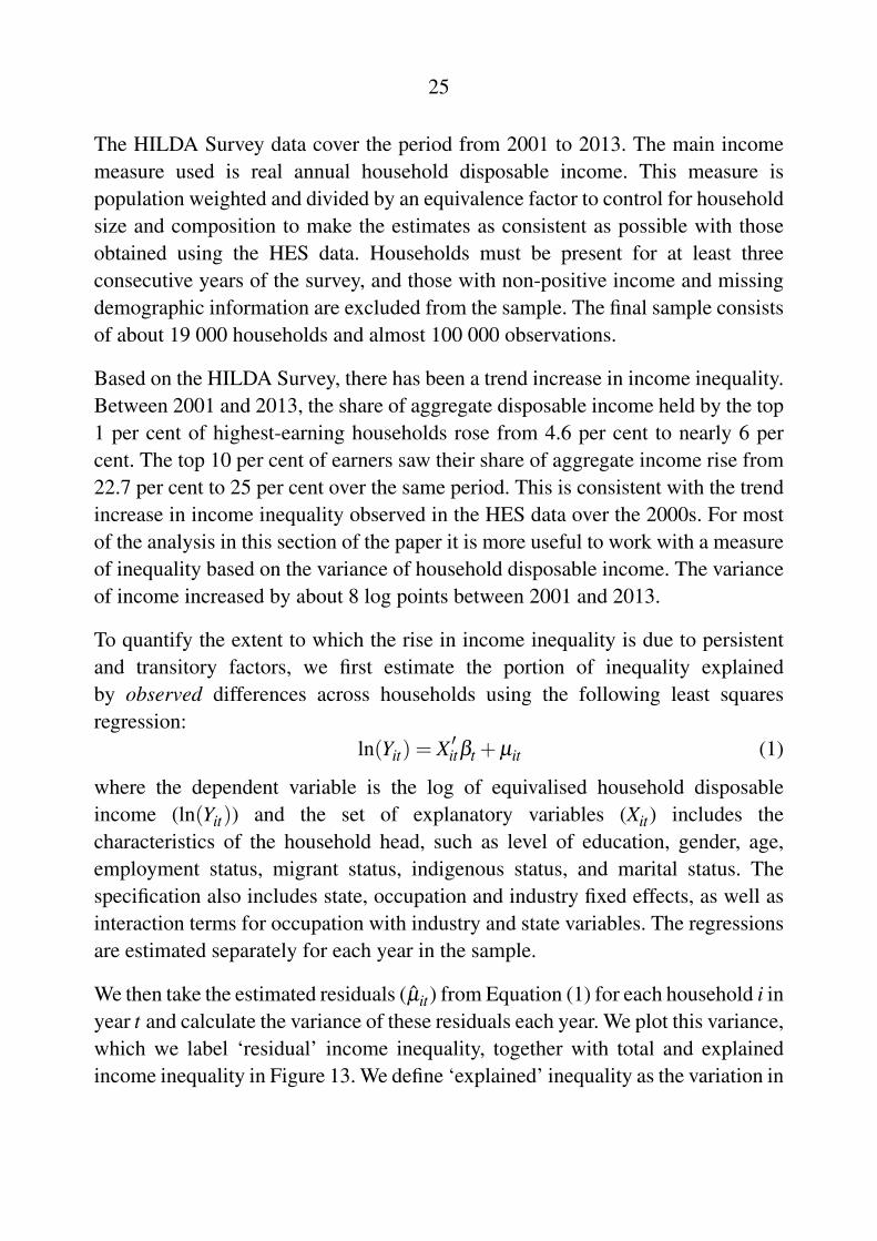
The HILDA Survey data cover the period from 2001 to 2013. The main incomemeasure used is real annual household disposable income. This measure ispopulation weighted and divided by an equivalence factor to control for householdsize and composition to make the estimates as consistent as possible with thoseobtained using the HES data. Households must be present for at least threeconsecutive years of the survey, and those with non-positive income and missingdemographic information are excluded from the sample. The final sample consistsof about 19 000 households and almost 100 000 observations.

Based on the HILDA Survey, there has been a trend increase in income inequality.Between 2001 and 2013, the share of aggregate disposable income held by the top1 per cent of highest-earning households rose from 4.6 per cent to nearly 6 percent. The top 10 per cent of earners saw their share of aggregate income rise from22.7 per cent to 25 per cent over the same period. This is consistent with the trendincrease in income inequality observed in the HES data over the 2000s. For mostof the analysis in this section of the paper it is more useful to work with a measureof inequality based on the variance of household disposable income. The varianceof income increased by about 8 log points between 2001 and 2013.

To quantify the extent to which the rise in income inequality is due to persistentand transitory factors, we first estimate the portion of inequality explainedby observed differences across households using the following least squaresregression:

ln(Yit) = X ′itβt +µit (1)

where the dependent variable is the log of equivalised household disposableincome (ln(Yit)) and the set of explanatory variables (Xit) includes thecharacteristics of the household head, such as level of education, gender, age,employment status, migrant status, indigenous status, and marital status. Thespecification also includes state, occupation and industry fixed effects, as well asinteraction terms for occupation with industry and state variables. The regressionsare estimated separately for each year in the sample.

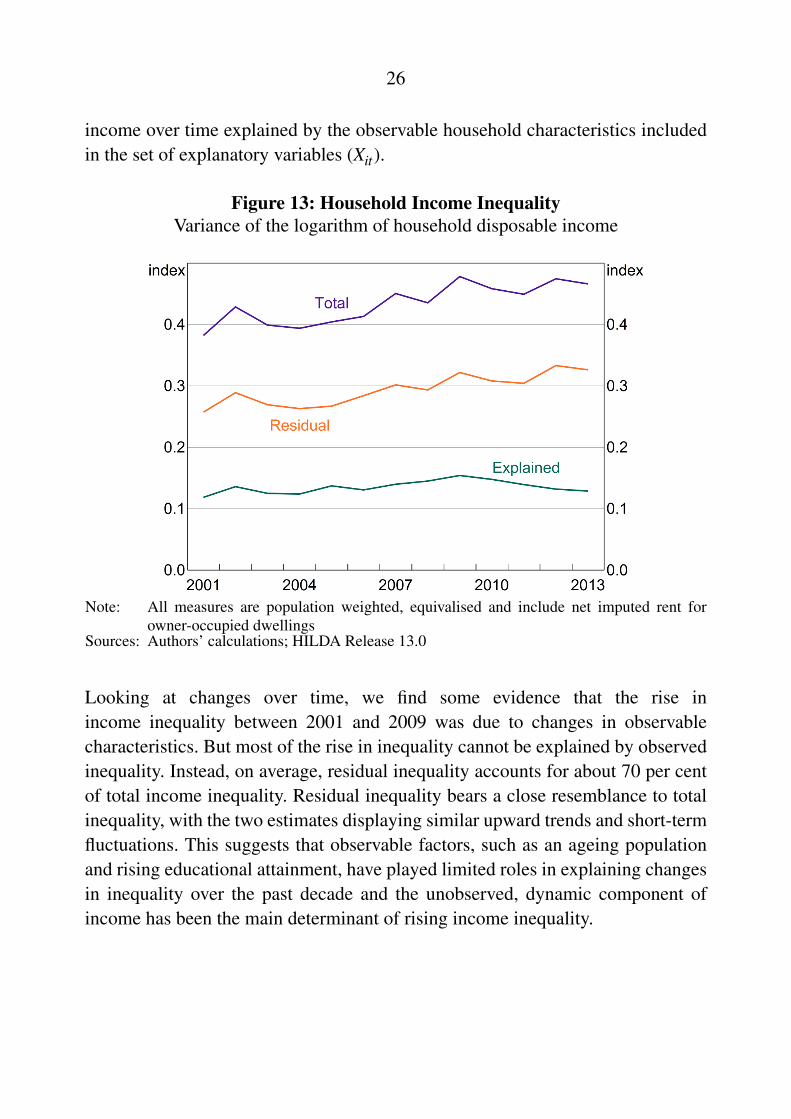
We then take the estimated residuals (µit) from Equation (1) for each household i inyear t and calculate the variance of these residuals each year. We plot this variance,which we label ‘residual’ income inequality, together with total and explainedincome inequality in Figure 13. We define ‘explained’ inequality as the variation in

26

income over time explained by the observable household characteristics includedin the set of explanatory variables (Xit).

Figure 13: Household Income InequalityVariance of the logarithm of household disposable income

Note: All measures are population weighted, equivalised and include net imputed rent forowner-occupied dwellings

Sources: Authors’ calculations; HILDA Release 13.0

Looking at changes over time, we find some evidence that the rise inincome inequality between 2001 and 2009 was due to changes in observablecharacteristics. But most of the rise in inequality cannot be explained by observedinequality. Instead, on average, residual inequality accounts for about 70 per centof total income inequality. Residual inequality bears a close resemblance to totalinequality, with the two estimates displaying similar upward trends and short-termfluctuations. This suggests that observable factors, such as an ageing populationand rising educational attainment, have played limited roles in explaining changesin inequality over the past decade and the unobserved, dynamic component ofincome has been the main determinant of rising income inequality.

27

5.1 Error Components Model

We next use an error components model (ECM) to decompose residual incomeinequality. The ECM has been standard in the inequality literature sinceGottschalk and Moffitt (1994). Many international studies have used this modelto estimate the dynamics of inequality over time, particularly for the United Statesusing the Panel Study of Income Dynamics Survey.15 To date, this approach hasnot been possible for Australia due to the absence of a sufficiently long paneldataset.

To address this, we use the panel structure of the HILDA Survey and a flexiblespecification of the ECM to examine the dynamics of household income inequalityfor Australia.

As before, the residual of log equivalised disposable income for household i inyear t is estimated from the regression described by Equation (1). The dynamicsof the residual are then modelled by the following process:

µit = λtαi + zit + vitzit = ρzit−1 +ηitvit = εit +θεit−1

(2)

where the ‘persistent’ component of inequality is a combination of a householdfixed effect (αi) that has a time-varying coefficient (λt), with total variance ofλ

2t σ

2α , and a highly persistent term (zit) that follows an autoregressive AR(1)

process and has variance of σ2z . The household fixed effect captures unobserved

time-invariant factors such as skill or ability (i.e. human capital). The time-varyingcoefficient captures the ‘market price’ for human capital. The AR(1) term (zit)captures other shocks to income that persist over time, such as promotions thataffect the level of wage income or possibly a long-term health condition. Thetemporary component (vit) is specified as a moving average MA(1) process. Thisspecification allows temporary income factors, such as lay-offs and bonuses, tohave effects that persist for more than a year. This is motivated by empiricalobservation of the autocovariances of household income in the HILDA data.

15 Prominent examples include MaCurdy (1982), Abowd and Card (1989), Blundell, Pistaferriand Preston (2008) and Heathcote et al (2010).

28

The ηit and εit terms are the respective persistent and transitory shocks to incomewith mean zero and time-varying variances, σ

2ηt and σ

2εt , respectively. These

shocks are assumed to be uncorrelated with each other and independently andidentically distributed across households over time. Under this error scheme,changes in residual inequality can be driven by changes in three different factors:1) the variance of persistent shocks; 2) the variance of temporary shocks; and/or3) changes in the market price of a household’s fixed human capital.

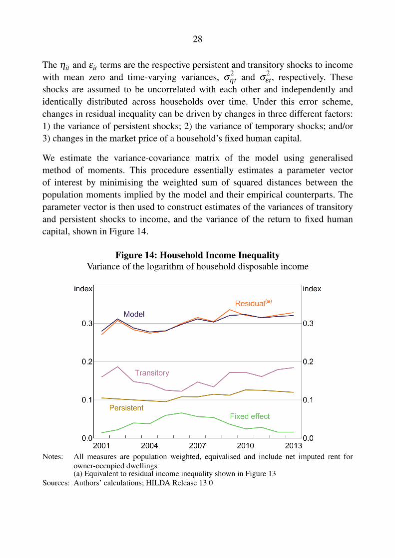
We estimate the variance-covariance matrix of the model using generalisedmethod of moments. This procedure essentially estimates a parameter vectorof interest by minimising the weighted sum of squared distances between thepopulation moments implied by the model and their empirical counterparts. Theparameter vector is then used to construct estimates of the variances of transitoryand persistent shocks to income, and the variance of the return to fixed humancapital, shown in Figure 14.

Figure 14: Household Income InequalityVariance of the logarithm of household disposable income

Notes: All measures are population weighted, equivalised and include net imputed rent forowner-occupied dwellings(a) Equivalent to residual income inequality shown in Figure 13

Sources: Authors’ calculations; HILDA Release 13.0

29

Our preferred estimates indicate that about two-thirds of the level of residualinequality is due to the variance in transitory income shocks. Given that about70 per cent of the variation in total income across households is due to unobservedcharacteristics, this suggests that temporary shocks explain close to one-half ofthe total cross-sectional variation in household income. The remaining variationin income across households is mainly due to variation in persistent shocks, thoughsome inequality is also explained by variation in unobserved fixed human capital.

The model also indicates that the first half of the sample period (2001 to 2006)was characterised by a slight decline in transitory income inequality and a small(and largely offsetting) increase in persistent income inequality (due to an increasein the variance of the fixed effect). This appears to reflect developments in theAustralian labour market over that period. In particular, the unemployment ratefell noticeably between 2001 and 2006 and this is likely to have disproportionatelybenefited lower-income workers who may be more exposed to temporary incomeshocks. The increase in the variance of the fixed effect in the early to mid 2000sreflects a rise in the ‘price’ that the market was willing to pay for unobservedability, which may also be due to the relatively strong labour market at the time.

The trend in overall income inequality in the latter half of the sample periodappears to reflect an increase in the variance of both transitory and persistentincome shocks. There also appears to be a slight jump in transitory incomeinequality around the time of the global financial crisis. This suggests that thecrisis had a limited effect on the distribution of consumption across households.In general, households are more able to insulate their consumption from transitoryrather than persistent shocks to income. The slight rise in the variance of persistentincome shocks since the middle of the 2000s is consistent with the small increasein consumption inequality reported in the HES over a similar period.

5.2 Income Mobility

To further quantify the extent to which the trends in inequality are persistent wenext estimate the degree of mobility in the income distribution. Income mobilityhas a direct bearing on the degree of persistence in inequality. For example, ifhousehold income is relatively immobile and the same households are rankedas high-income from one year to the next, then this suggests that the inequalityis persistent. In contrast, if household income is fairly mobile on average then

30

high-income households may move down the income rankings the following year,suggesting that the inequality is temporary.

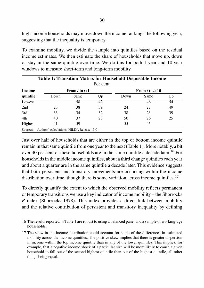
To examine mobility, we divide the sample into quintiles based on the residualincome estimates. We then estimate the share of households that move up, downor stay in the same quintile over time. We do this for both 1-year and 10-yearwindows to measure short-term and long-term mobility.

Table 1: Transition Matrix for Household Disposable IncomePer cent

Income From t to t+1 From t to t+10quintile Down Same Up Down Same UpLowest 58 42 46 542nd 23 38 39 24 27 493rd 33 34 32 38 23 394th 40 37 23 50 26 25Highest 41 59 55 45Sources: Authors’ calculations; HILDA Release 13.0

Just over half of households that are either in the top or bottom income quintileremain in that same quintile from one year to the next (Table 1). More notably, a bitover 40 per cent of these households are in the same quintile a decade later.16 Forhouseholds in the middle income quintiles, about a third change quintiles each yearand about a quarter are in the same quintile a decade later. This evidence suggeststhat both persistent and transitory movements are occurring within the incomedistribution over time, though there is some variation across income quintiles.17

To directly quantify the extent to which the observed mobility reflects permanentor temporary transitions we use a key indicator of income mobility – the ShorrocksR index (Shorrocks 1978). This index provides a direct link between mobilityand the relative contribution of persistent and transitory inequality by defining

16 The results reported in Table 1 are robust to using a balanced panel and a sample of working-agehouseholds.

17 The skew in the income distribution could account for some of the differences in estimatedmobility across the income quintiles. The positive skew implies that there is greater dispersionin income within the top income quintile than in any of the lower quintiles. This implies, forexample, that a negative income shock of a particular size will be more likely to cause a givenhousehold to fall out of the second highest quintile than out of the highest quintile, all otherthings being equal.

31

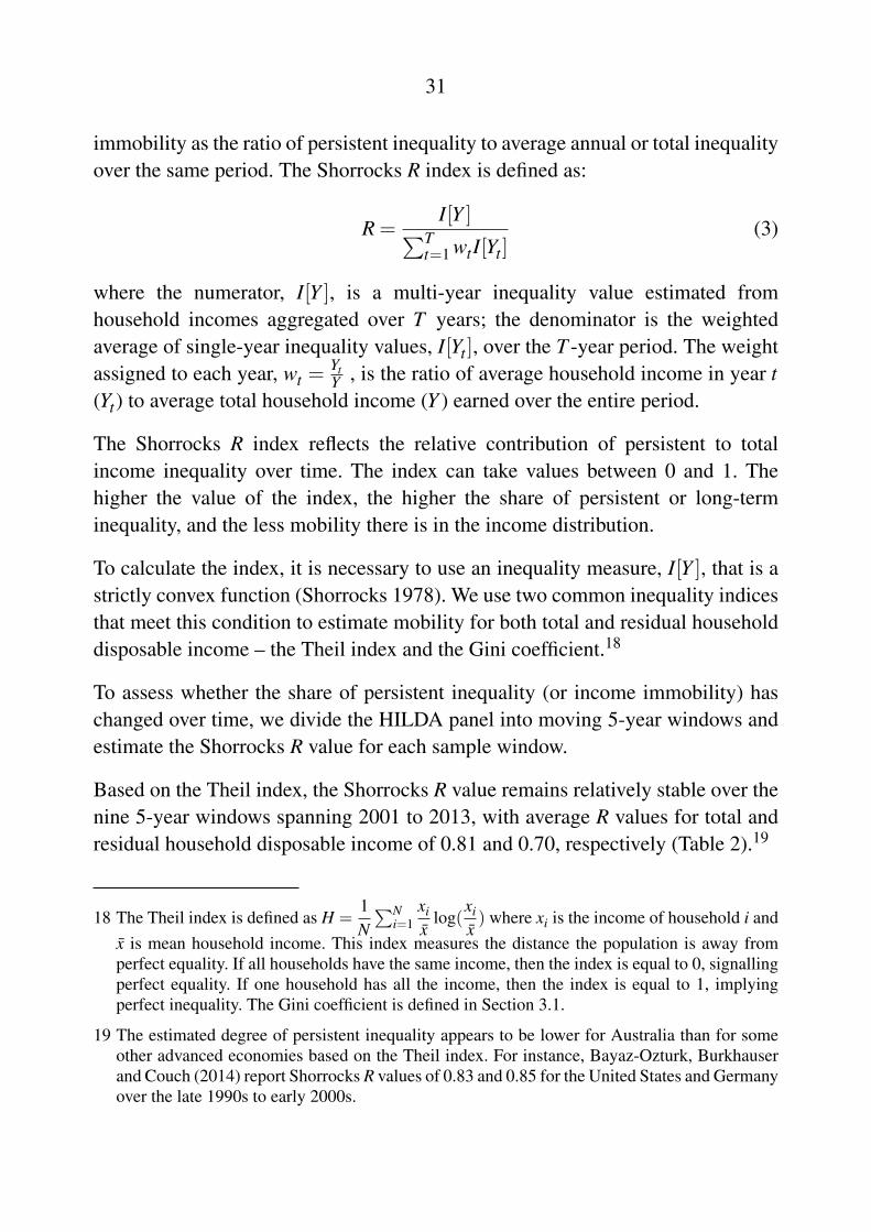
immobility as the ratio of persistent inequality to average annual or total inequalityover the same period. The Shorrocks R index is defined as:

R =I[Y ]∑T

t=1 wtI[Yt ](3)

where the numerator, I[Y ], is a multi-year inequality value estimated fromhousehold incomes aggregated over T years; the denominator is the weightedaverage of single-year inequality values, I[Yt ], over the T -year period. The weightassigned to each year, wt =

YtY , is the ratio of average household income in year t

(Yt) to average total household income (Y ) earned over the entire period.

The Shorrocks R index reflects the relative contribution of persistent to totalincome inequality over time. The index can take values between 0 and 1. Thehigher the value of the index, the higher the share of persistent or long-terminequality, and the less mobility there is in the income distribution.

To calculate the index, it is necessary to use an inequality measure, I[Y ], that is astrictly convex function (Shorrocks 1978). We use two common inequality indicesthat meet this condition to estimate mobility for both total and residual householddisposable income – the Theil index and the Gini coefficient.18

To assess whether the share of persistent inequality (or income immobility) haschanged over time, we divide the HILDA panel into moving 5-year windows andestimate the Shorrocks R value for each sample window.

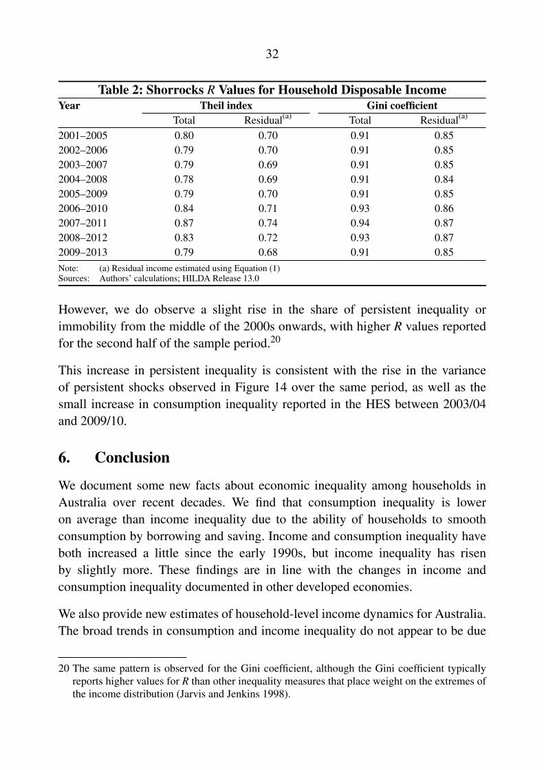
Based on the Theil index, the Shorrocks R value remains relatively stable over thenine 5-year windows spanning 2001 to 2013, with average R values for total andresidual household disposable income of 0.81 and 0.70, respectively (Table 2).19

18 The Theil index is defined as H =1N∑N

i=1xi

xlog(

xi

x) where xi is the income of household i and

x is mean household income. This index measures the distance the population is away fromperfect equality. If all households have the same income, then the index is equal to 0, signallingperfect equality. If one household has all the income, then the index is equal to 1, implyingperfect inequality. The Gini coefficient is defined in Section 3.1.

19 The estimated degree of persistent inequality appears to be lower for Australia than for someother advanced economies based on the Theil index. For instance, Bayaz-Ozturk, Burkhauserand Couch (2014) report Shorrocks R values of 0.83 and 0.85 for the United States and Germanyover the late 1990s to early 2000s.

32

Table 2: Shorrocks R Values for Household Disposable IncomeYear Theil index Gini coefficient

Total Residual(a) Total Residual(a)

2001–2005 0.80 0.70 0.91 0.852002–2006 0.79 0.70 0.91 0.852003–2007 0.79 0.69 0.91 0.852004–2008 0.78 0.69 0.91 0.842005–2009 0.79 0.70 0.91 0.852006–2010 0.84 0.71 0.93 0.862007–2011 0.87 0.74 0.94 0.872008–2012 0.83 0.72 0.93 0.872009–2013 0.79 0.68 0.91 0.85Note: (a) Residual income estimated using Equation (1)Sources: Authors’ calculations; HILDA Release 13.0

However, we do observe a slight rise in the share of persistent inequality orimmobility from the middle of the 2000s onwards, with higher R values reportedfor the second half of the sample period.20

This increase in persistent inequality is consistent with the rise in the varianceof persistent shocks observed in Figure 14 over the same period, as well as thesmall increase in consumption inequality reported in the HES between 2003/04and 2009/10.

6. Conclusion

We document some new facts about economic inequality among households inAustralia over recent decades. We find that consumption inequality is loweron average than income inequality due to the ability of households to smoothconsumption by borrowing and saving. Income and consumption inequality haveboth increased a little since the early 1990s, but income inequality has risenby slightly more. These findings are in line with the changes in income andconsumption inequality documented in other developed economies.

We also provide new estimates of household-level income dynamics for Australia.The broad trends in consumption and income inequality do not appear to be due

20 The same pattern is observed for the Gini coefficient, although the Gini coefficient typicallyreports higher values for R than other inequality measures that place weight on the extremes ofthe income distribution (Jarvis and Jenkins 1998).

33

to changes in observed household characteristics, but rather to changes in thedistribution of unobserved shocks. The increase in income inequality over thepast decade has reflected similar-sized increases in the variance of transitory andpersistent income shocks. The rise in persistent income inequality since the middleof the 2000s is consistent with the rise in consumption inequality over the sameperiod.

Our results also suggest that monetary policy can affect inequality to the extentthat changes in interest rates influence asset prices, and such interest-sensitiveassets are not distributed equally across the household population. But our resultsalso indicate that the direction of these effects is unclear a priori. For instance,lower interest rates may lead to higher housing prices which, in turn, boostwealth inequality given that wealthy households are more likely to own theirhomes. But if income and spending are adjusted to account for imputed rent, ourresults also imply that lower interest rates could boost imputed rent (relative tomarket rents) and disproportionately benefit relatively low-income home owners,reducing measured inequality in income and consumption, at least in the shortterm.

34

Appendix A: Imputed Rent and the Distributions of HouseholdExpenditure and Income

To understand how the addition of imputed rent affects the measured distributionsof consumption and income it helps to consider some simple accounting exercises.

Suppose a renter has the following single period budget constraint:

E +R = (Y −T )−S

Where total expenditure consists of non-housing expenditure (E) and expenditureon housing services which, for the renter, is simply the value of market rent paid(R). The total resources available each period consist of non-housing income (Y ),such as wages and salaries, less net government taxes (T ) and saving (S).

A home owner has a corresponding budget constraint:

E +M = (Y −T )−S

This expression is essentially the same as that of the renter, except that the housingexpenditure of the home owner is given by mortgage interest payments (and othercosts of maintaining a home) (M). Now suppose we add gross imputed rent (IR) toboth sides of the home owner’s budget constraint (and just move mortgage interestpayments to the right of the constraint):

E + IR = (Y −T )+(IR−M)−S

Now the home owner spends an amount equal to gross imputed rent on housingservices and earns ‘housing income’ measured by net imputed rent (which is justgross imputed rent less mortgage interest payments) (NIR= IR−M). The additionof gross imputed rent to both sides of the household budget constraint does notaffect aggregate household saving. But it affects the distribution of both spendingand income if home owners are not identical to renters.21

In essence, we add net imputed rent to non-housing expenditure when we redefinehousehold ‘expenditure’ as ‘consumption’. In other words, we replace mortgage

21 We could also write down the budget constraint for a housing investor but it does not affect theoverall story.

35

interest payments (and associated housing costs, such as maintenance) with grossimputed rent. This causes measured inequality to fall because it affects low-spending households by more than high-spending households.

To demonstrate how consumption and expenditure inequality can follow differenttrends over time, consider the following simple decomposition.

Suppose that the level of imputed rent (IR) is simply given by the imputed rentalyield (r) multiplied by the housing price (HP):

IR = r ∗HP

Correspondingly, the level of mortgage interest payments (M) is equal to themortgage interest rate (i) multiplied by the outstanding stock of mortgage debt(D):

M = i∗D

It follows that we can write net imputed rent (as a share of income) as:

NIR/(Y +NIR) = (r− i∗D)/HP∗ (HP/(Y +NIR))

This decomposition shows that the distribution of net imputed rent (relative to totalincome) is a function of the distribution of three factors:

1. The ‘spread’ between the imputed rental yield and the mortgage interest rate(r− i)

2. The housing debt-to-price (or ‘leverage’) ratio (D/HP)

3. The house price-to-income ratio (HP/(Y +NIR)).

Changes in any of these factors can drive differential changes in measures ofinequality based on consumption and expenditure over time. Furthermore, theydrive changes in measures of income, depending on whether the estimates adjustfor net imputed rent or not.

36

Appendix B: Alternative Survey Measures of Inequality

In this Appendix we adopt an alternative definition of imputed rent to cross-checkthe results for consumption and income inequality in the paper.

B.1 Hedonic Estimates of Imputed Rent

The alternative measure of imputed rent is calculated using the ABS hedonicmodelling methodology, which estimates the market value of the rental equivalentfor owner-occupied dwellings using the dwelling characteristics available in theHES.

The dependent variable is the logarithm of gross imputed rent for the sample ofowner-occupier households.22 There are two types of explanatory variables in themodel – Type I and Type II variables.

The Type I variables describe the characteristics of the dwelling, including:23

• State

• Section of state (i.e. capital city or balance of state)

• Type of dwelling structure

• Number of bedrooms.

The Type II variables describe the households renting the dwellings, including:24

• Household income

• Type of landlord (i.e. public or private landlord).

22 The explanatory variables used to estimate the market rent are not as extensive as those used bythe ABS as we only have access to the basic confidentialised unit record files.

23 Prior to the 2003/04 survey, the ‘section of state’ variable is not included. The ‘state’ variableis not included in the 1988/89 survey.

24 Prior to the 2003/04 survey, landlord type is not included so we use tenure type to capturesimilar information.

37

The model for market renters is:

ln(Ri) = α0 +J∑

j=1

β jXi j +K∑

k=1

δkZik +φMi + εi

where ln(Ri) is the natural logarithm of the weekly rent of household i, Xi j is theset of Type I variables and Zik is the set of Type II variables for each household,Mi is the estimated Inverse Mills ratio and εi is a normally distributed error termwith a mean of zero and a standard deviation of σ .

The Inverse Mills ratio is calculated using the Heckman procedure. This adjusts forpossible bias that could result from non-random selection. The Inverse Mills ratiois the ratio of the probability distribution function and the cumulative distributionfunction of the standard Z-score estimated in the probit model:

P(i ∈ ‘renter’) = Φ(Xβ )

where X is a set of dwelling and household characteristics (e.g. age andeducational attainment of household head) that determine whether a householdrents or not.25

Next, we make an adjustment to the intercept to control for the Type II variables.Specifically, the intercept is adjusted to the mean for renters:

αad j0 = α0 +

K∑k=1

δkZk

where αad j0 is the adjusted intercept for imputation, α0 is the intercept estimate of

the basic model, δk is the estimated coefficient for each Type II variable, and Zk isthe mean of each Type II variable.

A scaling factor is then applied to preserve the relationship between the observedand model rent estimates for private market renters. The imputed rent distributionis re-positioned to the original median rent observed in the private market renters’data.

ScalingFactor = median(R)−median(Rrenter)

25 Prior to 1998/99, the education variable is not included.

38

and so:ROODad j

i = ROODi +ScalingFactor

where ROODi is the estimated gross imputed rent for owner-occupier household i.

Since the model does not fully explain the variation in rent for high-valuedwellings, an extrapolation method is used to adjust gross imputed rent forhigh-value dwellings. A ceiling rent is determined by a visual inspection of themodelled results. The ceiling rent is divided by the estimated annual average rateof return for all owners. A regression model is fitted to owners below the housevalue cut-off:

ri = θ0 +θ11hi+θ2(

1hi)2 + εi

where ri =ROODad j

ihi

is the rental rate of return for owner-occupier household i andhi is the value of that household’s dwelling.

The gross imputed rent for owners with house values above the cut-off wererecalculated using the statistically significant coefficients in the above equation.The extrapolated imputed rent is given by:26

ROODhighvaluej = p jr j

where ROODhighvaluej is the adjusted gross imputed rent for the jth owner-occupied

dwelling, p j is the jth home value and r j is the estimated rental rate of return. Forfurther details, see Australian Bureau of Statistics (2008).

B.2 Alternative Estimates of Inequality

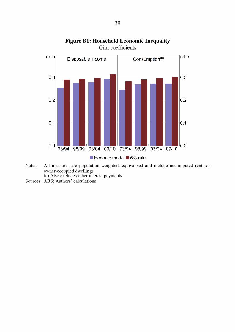
Using the alternative measure of imputed rent results in a lower level of inequalityfor both income and consumption (as measured by the Gini coefficient) comparedwith the simple approach in the main paper (Figure B1). The upward trend fordisposable income inequality is apparent under both approaches. However, the risein consumption inequality is less apparent under the hedonic modelling approach.

26 We are not able to use this extrapolation method for the 1975/76, 1984 and 1988/89 surveysbecause the estimated housing value of the dwelling is not included.

39

Figure B1: Household Economic InequalityGini coefficients



40

Appendix C: Income Inequality Estimates Using Tax Records

Income tax records provide an alternative way of measuring income inequality.These estimates are useful because tax records typically cover a broaderpopulation of individuals than household surveys (and hence better capture topincome earners). There is also a long and consistent history of tax records,providing us with a sense of long-run trends. The main limitations of tax datarelative to household surveys are that we generally cannot examine the underlyingcharacteristics that are driving any changes over time and we can only measureinequality in individual incomes.

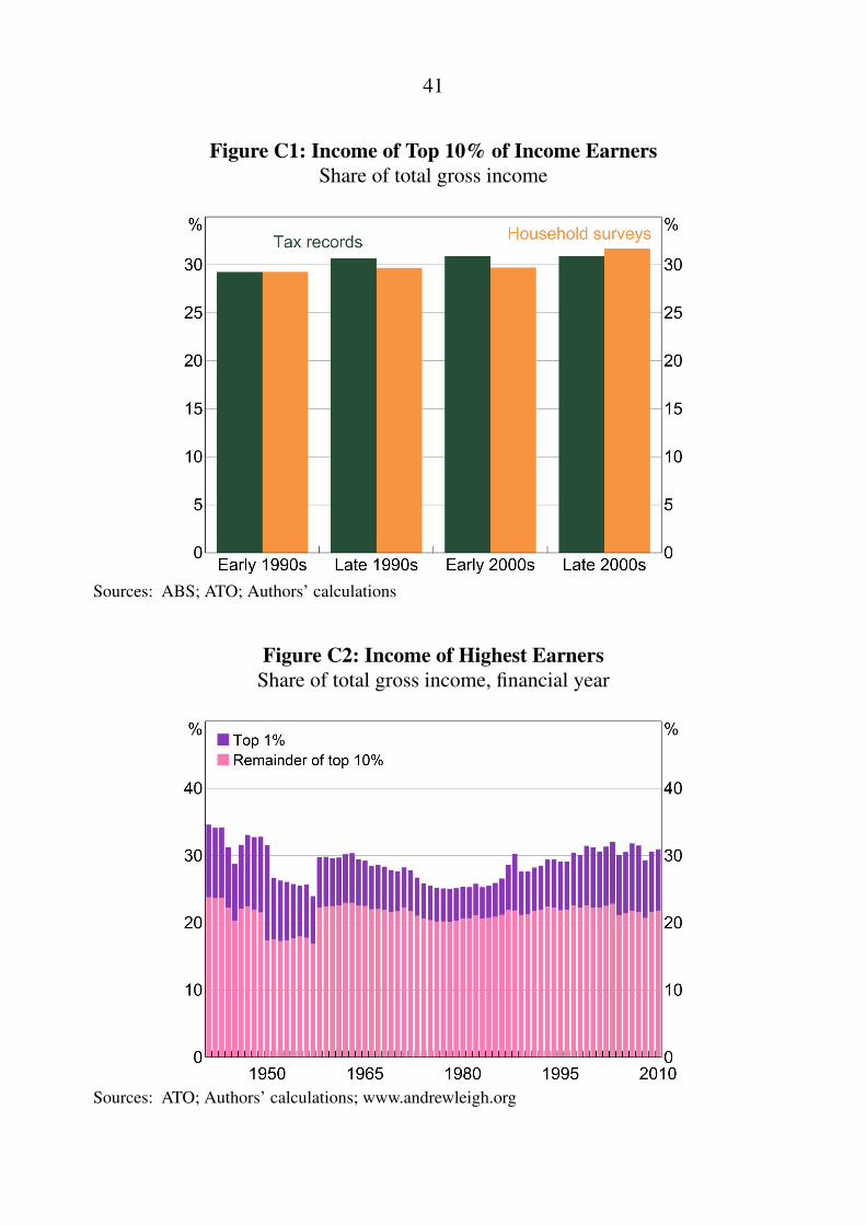
Estimates of individual income inequality based on tax records are very similar tothose based on the SIH data (Figure C1). Since the early 1990s, relative to the taxrecords, the survey data has underestimated the share of income going to the top 10per cent of earners by about 0.4 percentage points, on average. This suggests thatthe analysis based on the survey data is reasonably representative of the broaderpopulation of individuals covered by the tax data. Moreover, the consistency overtime between the two series suggests that the survey data captures genuine trendsin income inequality.27

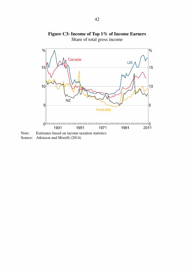
Using the Australian tax data, Leigh (2013) shows that the top shares in grossincome follow a U-shape, decreasing from the early 1940s to the 1980s andthen increasing after this period (Figure C2). To put this in an internationalcontext, cross-country comparisons can be made using the tax data collected byAtkinson and Morelli (2014). It is clear from Figure C3 that the U-shape pattern iscommon to several developed Anglo-Saxon countries, such as the United States,the United Kingdom, New Zealand and Canada (Atkinson and Morelli 2014). Incontrast, the share of aggregate income accruing to the highest income earners hasremained fairly steady since the 1950s in countries such as France, Germany andJapan (Piketty 2014).

27 For a more complete discussion of the uses and limitations of tax and survey data, seeWilkins (2013).

41

Figure C1: Income of Top 10% of Income EarnersShare of total gross income

Sources: ABS; ATO; Authors’ calculations

Figure C2: Income of Highest EarnersShare of total gross income, financial year

Sources: ATO; Authors’ calculations; www.andrewleigh.org

42

Figure C3: Income of Top 1% of Income EarnersShare of total gross income

Note: Estimates based on income taxation statisticsSource: Atkinson and Morelli (2014)

43

References

Abowd JM and D Card (1989), ‘On the Covariance Structure of Earnings andHours Changes’, Econometrica, 57(2), pp 411–445.

Aguiar MA and M Bils (2011), ‘Has Consumption Inequality Mirrored IncomeInequality?’, NBER Working Paper No 16807.

Atkinson AB and S Morelli (2014), ‘Chartbook of Economic Inequality’, Societyfor the Study of Economic Inequality Working Paper ECINEQ WP 20014 - 324.

Attanasio O, E Hurst and L Pistaferri (2014), ‘The Evolution of Income,Consumption, and Leisure Inequality in the United States, 1980–2010’, inCD Carroll, TF Crossley and J Sabelhaus (eds), Improving the Measurement ofConsumer Expenditures, NBER Studies in Income and Wealth, Vol 74, Universityof Chicago Press, Chicago, pp 100–140.

Australian Bureau of Statistics (2008), ‘Experimental Estimates of ImputedRent, Australia, 2003-04 and 2005-06’, ABS Cat No 6525.0.

Barrett G, TF Crossley and C Worswick (1999), ‘Consumption and IncomeInequality in Australia’, Australian National University Centre for EconomicPolicy Research Discussion Paper No 404.

Bayaz-Ozturk G, RV Burkhauser and KA Couch (2014), ‘Consolidatingthe Evidence on Income Mobility in the Western States of Germany and theUnited States from 1984 to 2006’, Economic Inquiry, 52(1), pp 431–443.

Beech A, R Dollman, R Finlay and G La Cava (2014), ‘The Distribution ofHousehold Spending in Australia’, RBA Bulletin, March, pp 13–22.

Blundell R and B Etheridge (2010), ‘Consumption, Income and EarningsInequality in Britain’, Review of Economic Dynamics, 13(1), pp 76–102.

Blundell R, L Pistaferri and I Preston (2008), ‘Consumption Inequality andPartial Insurance’, The American Economic Review, 98(5), pp 1887–1921.

44

Bray JR (2014), ‘Changes in Inequality in Australia and the RedistributionalImpacts of Taxes and Government Benefits’, in A Podger and D Trewin (eds),Measuring and Promoting Wellbeing: How Important is Economic Growth?:Essays in Honour of Ian Castles AO and a Selection of Castle’s Papers, Australiaand New Zealand School of Government Monograph, ANU Press, Canberra,pp 423–475.

Brzozowski M, M Gervais, P Klein and M Suzuki (2010), ‘Consumption,Income, and Wealth Inequality in Canada’, Review of Economic Dynamics, 13(1),pp 52–75.

DeBacker J, B Heim, V Panousi, S Ramnath and I Vidangos (2013), ‘RisingInequality: Transitory or Persistent? New Evidence from a Panel of U.S. TaxReturns’, Brookings Papers on Economic Activity, Spring, pp 67–122.

Domeij D and M Floden (2010), ‘Inequality Trends in Sweden 1978–2004’,Review of Economic Dynamics, 13(1), pp 179–208.

Fletcher M and B Guttmann (2013), ‘Income Inequality in Australia’, EconomicRoundup, 2, pp 35–54.

Friedman M (1957), A Theory of the Consumption Function, NBER GeneralSeries, No 63, Princeton University Press, Princeton.

Fuchs-Schundeln N, D Krueger and M Sommer (2010), ‘Inequality Trends forGermany in the Last Two Decades: A Tale of Two Countries’, Review of EconomicDynamics, 13(1), pp 103–132.

Gottschalk P and R Moffitt (1994), ‘The Growth of Earnings Instabilityin the U.S. Labor Market’, Brookings Papers on Economic Activity, 1994(2),pp 217–254, 270–272.

Greenville J, C Pobke and N Rogers (2013), Trends in the Distribution ofIncome in Australia, Productivity Commission Staff Working Paper, ProductivityCommission, Canberra.

Harding A and H Greenwell (2002), ‘Trends in Income and ConsumptionInequality in Australia’, Paper presented at the 27th General Conference ofthe International Association for Research in Income and Wealth, Stockholm,18–24 August.

45

Heathcote J, F Perri and GL Violante (2010), ‘Unequal We Stand: An EmpiricalAnalysis of Economic Inequality in the United States: 1967–2006’, Review ofEconomic Dynamics, 13(1), pp 15–51.

Jappelli T and L Pistaferri (2010), ‘Does Consumption Inequality Track IncomeInequality in Italy?’, Review of Economic Dynamics, 13(1), pp 133–153.

Jarvis S and SP Jenkins (1998), ‘How Much Income Mobility is There inBritain?’, The Economic Journal, 108(447), pp 428–443.

Krueger D and F Perri (2005), ‘Does Income Inequality Lead to ConsumptionEquality? Evidence and Theory’, Federal Reserve Bank of Minneapolis ResearchDepartment Staff Report No 363.

Krueger D, F Perri, L Pistaferri and GL Violante (2010), ‘Cross-SectionalFacts for Macroeconomists’, Review of Economic Dynamics, 13(1), pp 1–14.

Leigh A (2013), Battlers & Billionaires: The Story of Inequality in Australia,Redback, Collingwood.

MaCurdy TE (1982), ‘The Use of Time Series Processes to Model the ErrorStructure of Earnings in a Longitudinal Data Analysis’, Journal of Econometrics,18(1), pp 83–114.

Meyer BD and JX Sullivan (2012), ‘Winning the War: Poverty from the GreatSociety to the Great Recession’, Brookings Papers on Economic Activity, Fall,pp 133–183.

Pijoan-Mas J and V Sanchez-Marcos (2010), ‘Spain is Different: Falling Trendsof Inequality’, Review of Economic Dynamics, 13(1), pp 154–178.

Piketty T (2014), Capital in the Twenty-First Century, trans A Goldhammer, TheBelknap Press of Harvard University Press, Cambridge.

Saunders P and P Siminski (2005), ‘Home Ownership And Inequality:Imputed Rent And Income Distribution In Australia’, Economic Papers, 24(4),pp 346–367.

Shorrocks A (1978), ‘Income Inequality and Income Mobility’, Journal ofEconomic Theory, 19(2), pp 376–393.

46

Slesnick DT (1998), ‘Empirical Approaches to the Measurement of Welfare’,Journal of Economic Literature, 36(4), pp 2108–2165.

Wilkins R (2013), ‘Evaluating the Evidence on Income Inequality in Australia inthe 2000s’, Melbourne Institute Working Paper Series No 26/13.

Wilkins R (2015), ‘Measuring Income Inequality In Australia’, The AustralianEconomic Review, 48(1), pp 93–102.

Yates J (1994), ‘Imputed Rent and Income Distribution’, The Review of Incomeand Wealth, 40(1), pp 43–66.

47

Copyright and Disclaimer Notices

HILDA

The following Disclaimer applies to data obtained from the HILDA Survey andreported in this RDP.

Disclaimer

The Household, Income and Labour Dynamics in Australia (HILDA) Surveywas initiated and is funded by the Australian Government Department of SocialServices (DSS), and is managed by the Melbourne Institute of Applied Economicand Social Research (Melbourne Institute). The findings and views based on thesedata should not be attributed to either DSS or the Melbourne Institute.

Household Economic Inequality in Australia · Household Economic Inequality in Australia Rosetta...

Documents

Transcript of Household Economic Inequality in Australia · Household Economic Inequality in Australia Rosetta...