Household Demand and Supply - London School of...

Frank Cowell: Household Demand & Supply

HOUSEHOLD DEMAND AND SUPPLYMICROECONOMICSPrinciples and AnalysisFrank Cowell

Almost essential Consumer: Optimisation

Useful, but optionalFirm: Optimisation

Prerequisites

July 2017 1

Note: the detail in slides marked “ * ” can only be seen if you run the slideshow


Working out consumer responsesThe analysis of consumer optimisation gives us some

powerful tools:• The primal problem of the consumer is what we are really

interested in• Related dual problem can help us understand it• The analogy with the firm helps solve the dual

Use earlier work to map out the consumer's responses• to changes in prices • to changes in income

July 2017 2


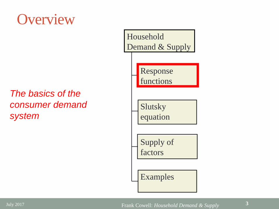
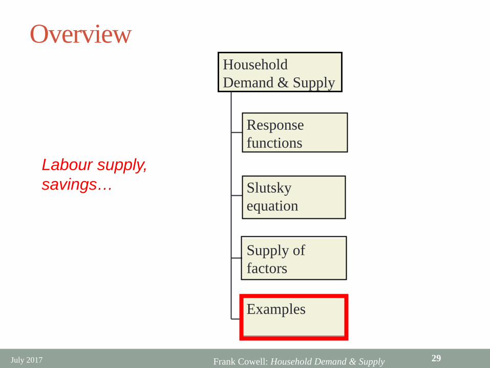
Overview

Response functions

Slutsky equation

Supply of factors

Examples

Household Demand & Supply

The basics of the consumer demand system

July 2017 3


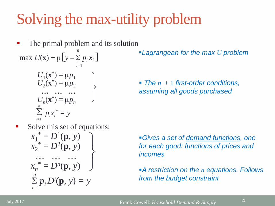
Solving the max-utility problem

n

Σ pixi* = y

i=1

U1(x*) = µp1U2(x*) = µp2

… … … Un(x*) = µpn

x1* = D1(p, y)

x2* = D2(p, y)

… … … xn

* = Dn(p, y)nΣ pi Di(p, y) = yi=1

The n + 1 first-order conditions, assuming all goods purchased

Gives a set of demand functions, one for each good: functions of prices and incomes

A restriction on the n equations. Follows from the budget constraint

Solve this set of equations:

The primal problem and its solutionn

max U(x) + µ[y – Σ pi xi ]i=1

Lagrangean for the max U problem

July 2017 4


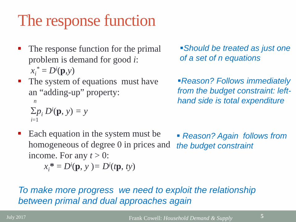
The response function The response function for the primal

problem is demand for good i:xi

* = Di(p,y)

Should be treated as just one of a set of n equations

The system of equations must have an “adding-up” property:

n

Σpi Di(p, y) = yi=1

Reason? Follows immediately from the budget constraint: left-hand side is total expenditure

Each equation in the system must be homogeneous of degree 0 in prices and income. For any t > 0:

xi* = Di(p, y )= Di(tp, ty)

Reason? Again follows from the budget constraint

To make more progress we need to exploit the relationship between primal and dual approaches again

July 2017 5


How you would use this in practice Consumer surveys

• data on expenditure for each household • over a number of categories of goods• perhaps income, hours worked as well

Market data are available on pricesGiven some assumptions about the structure of preferences

• estimate household demand functions for commodities• from this recover information about utility functions

July 2017 6


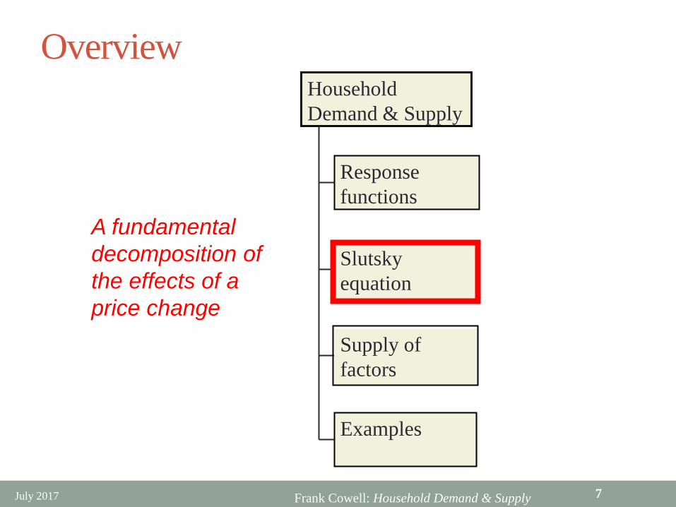
Overview

Response functions

Slutskyequation

Supply of factors

Examples


A fundamental decomposition of the effects of a price change

July 2017 7


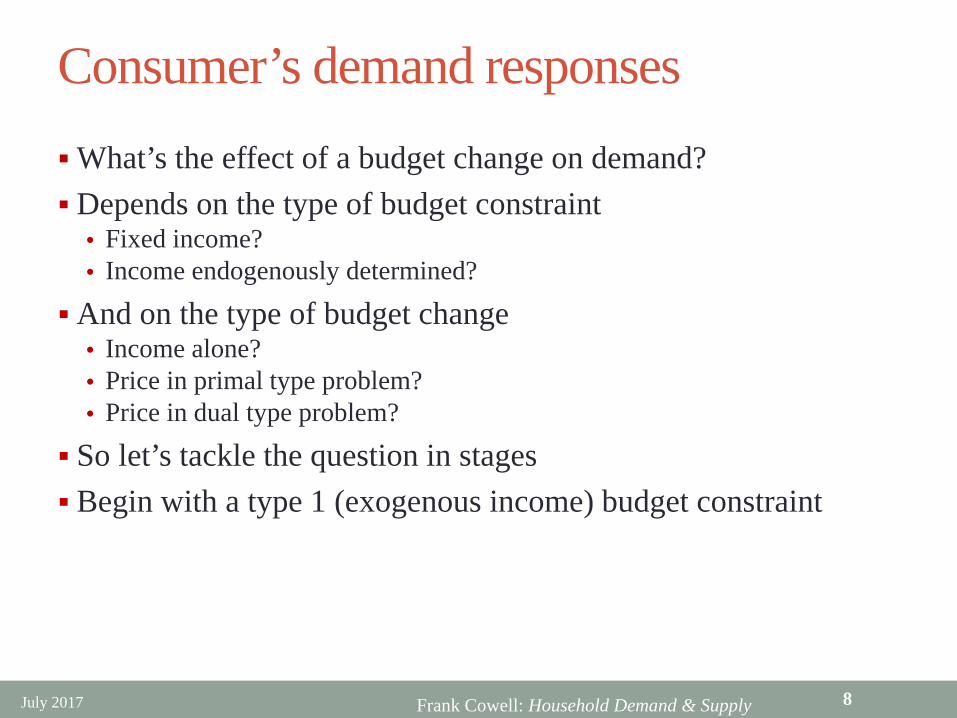
Consumer’s demand responsesWhat’s the effect of a budget change on demand? Depends on the type of budget constraint

• Fixed income?• Income endogenously determined?

And on the type of budget change• Income alone? • Price in primal type problem?• Price in dual type problem?

So let’s tackle the question in stages Begin with a type 1 (exogenous income) budget constraint

July 2017 8


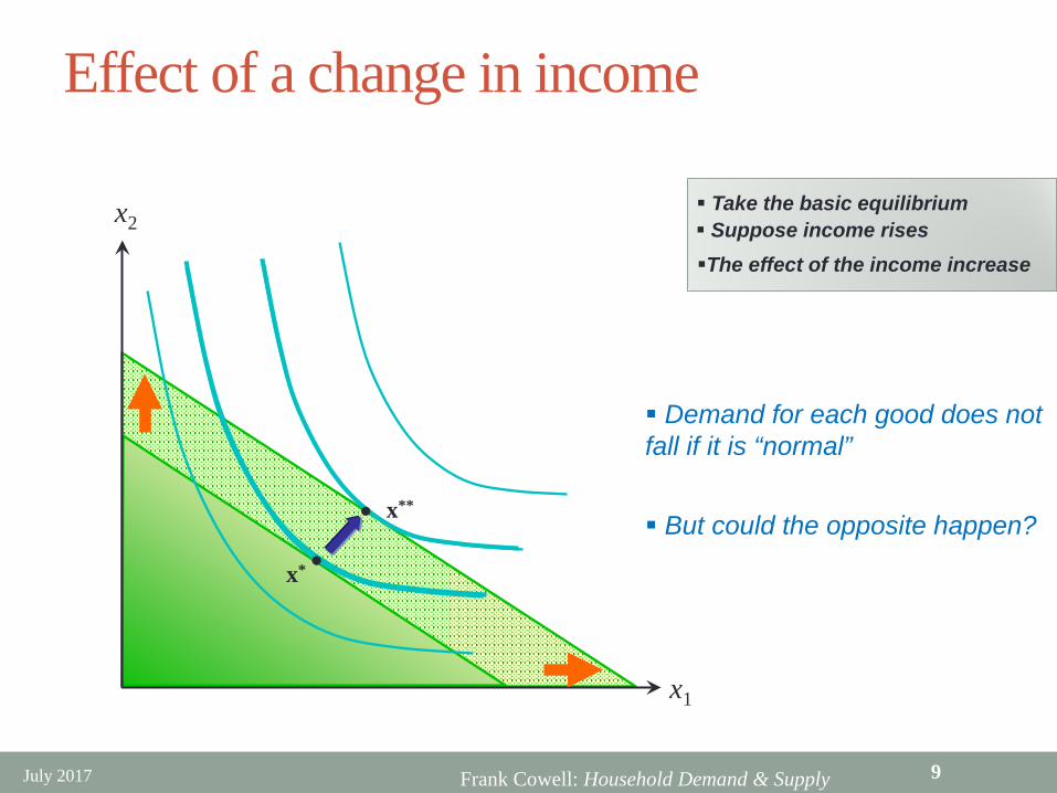
Effect of a change in income

x1

x*

Take the basic equilibrium Suppose income risesThe effect of the income increase

•

x**•

x2

Demand for each good does not fall if it is “normal”

But could the opposite happen?

July 2017 9


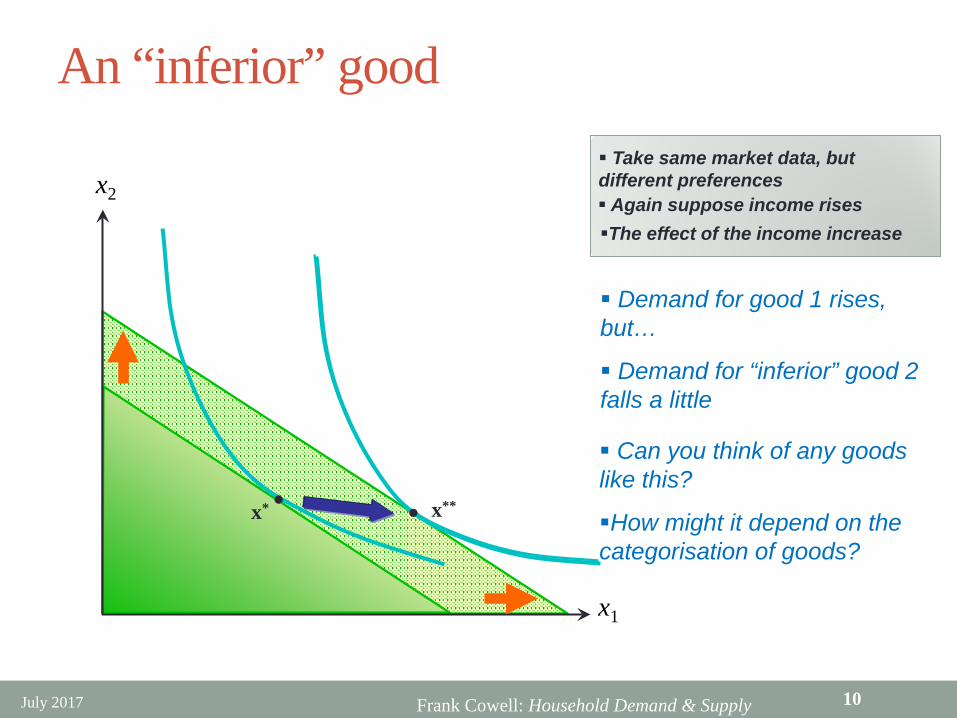
An “inferior” good

x1

x*

Take same market data, but different preferences Again suppose income risesThe effect of the income increase

•

x2

Demand for good 1 rises, but…

Demand for “inferior” good 2 falls a little

Can you think of any goods like this?

How might it depend on the categorisation of goods?

x**•

July 2017 10


A glimpse ahead…We can use the idea of an “income effect” in many applications Basic to an understanding of the effects of prices on the

consumer Because a price cut makes a person better off, as would an

income increase

July 2017 11


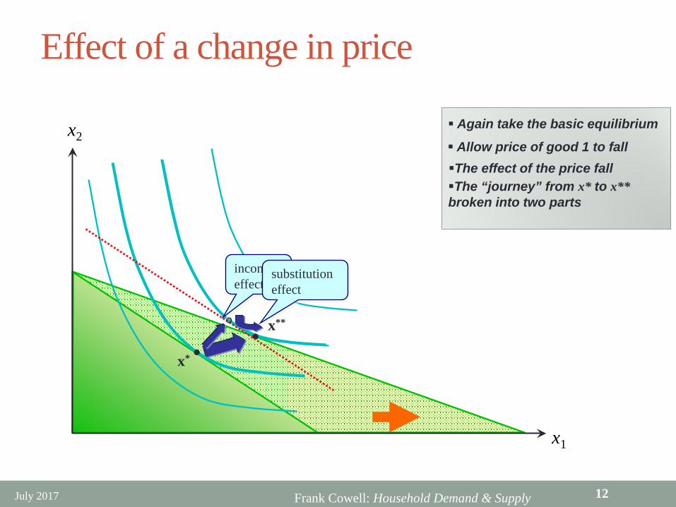
Effect of a change in price

x1

x*

Again take the basic equilibrium

Allow price of good 1 to fallThe effect of the price fall

•

x**•

x2

The “journey” from x* to x** broken into two parts

°

income effect

substitution effect

July 2017 12


And now let’s look at it in mathsWe want to take both primal and dual aspects of the problem……and work out the relationship between the response

functions…… using properties of the solution functions (Yes, it’s time for Shephard’s lemma again…)

July 2017 13


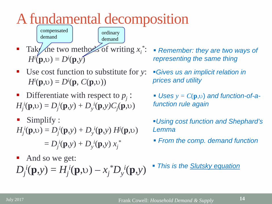
A fundamental decomposition

Take the two methods of writing xi*:

Hi(p,υ) = Di(p,y)

compensated demand

ordinary demand

Remember: they are two ways of representing the same thing

Use cost function to substitute for y:Hi(p,υ) = Di(p, C(p,υ))

Differentiate with respect to pj : Hj

i(p,υ) = Dji(p,y) + Dy

i(p,y)Cj(p,υ)

Gives us an implicit relation in prices and utility

Simplify : Hj

i(p,υ) = Dji(p,y) + Dy

i(p,y) Hj(p,υ)

Uses y = C(p,υ) and function-of-a-function rule again

Using cost function and Shephard’sLemma

= Dji(p,y) + Dy

i(p,y) xj* From the comp. demand function

And so we get:Dj

i(p,y) = Hji(p,υ) – xj

*Dyi(p,y) This is the Slutsky equation

July 2017 14


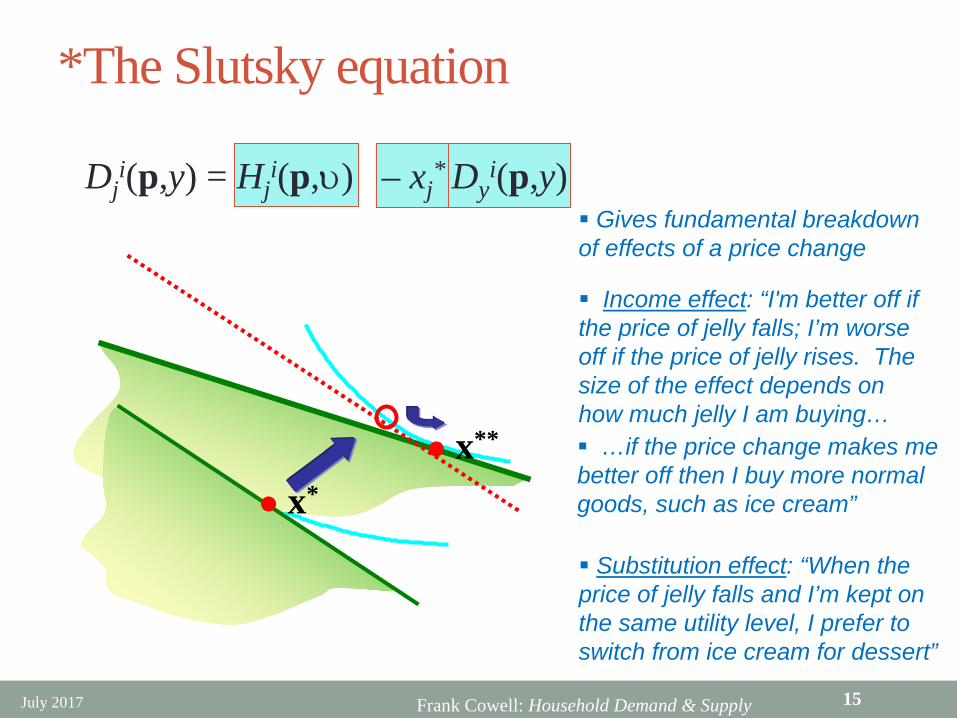
*The Slutsky equation

Gives fundamental breakdown of effects of a price change

Income effect: “I'm better off if the price of jelly falls; I’m worse off if the price of jelly rises. The size of the effect depends on how much jelly I am buying…

Substitution effect: “When the price of jelly falls and I’m kept on the same utility level, I prefer to switch from ice cream for dessert”

x**

Dji(p,y) = Hj

i(p,υ) – xj* Dy

i(p,y)

x*

July 2017 15

…if the price change makes me better off then I buy more normal goods, such as ice cream”


Slutsky: Points to watch Income effects for some goods may have “wrong” sign

• for inferior goods…• …get opposite effect to that on previous slide

For n > 2 the substitution effect for some pairs of goods could be positive • net substitutes• apples and bananas?

While that for others could be negative• net complements• gin and tonic?

Neat result is available if we look at special case where j = i

July 2017 16


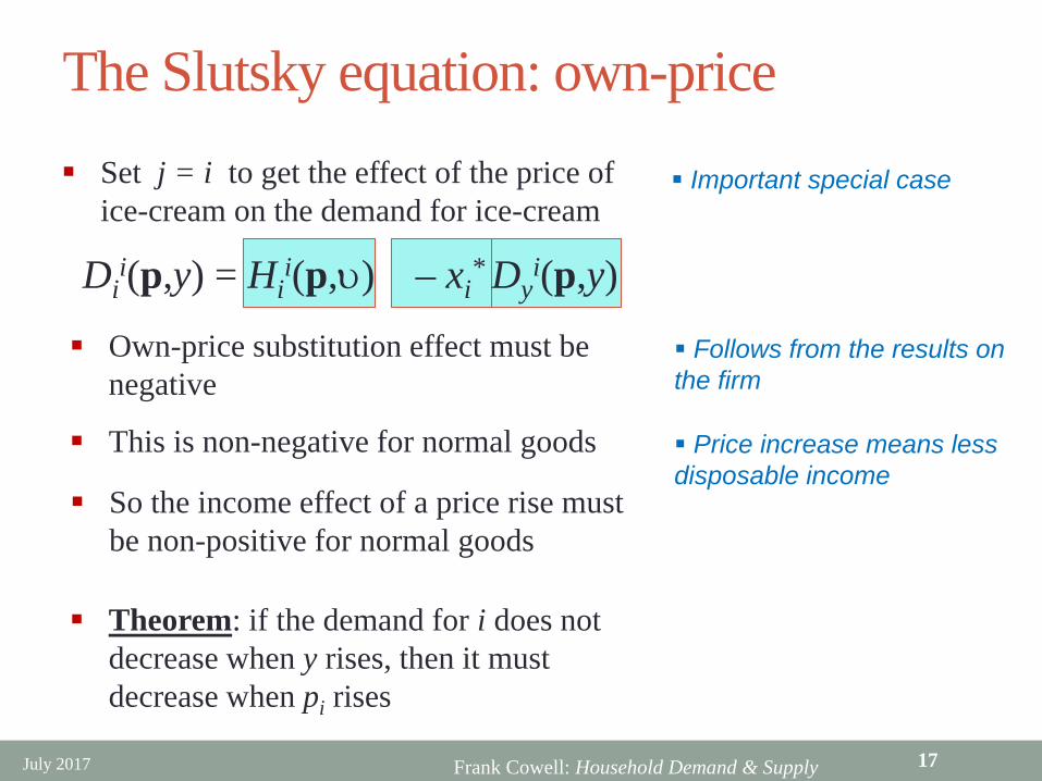
The Slutsky equation: own-price

Dii(p,y) = Hi

i(p,υ) – xi* Dy

i(p,y)

Set j = i to get the effect of the price of ice-cream on the demand for ice-cream

Own-price substitution effect must be negative

This is non-negative for normal goods

Theorem: if the demand for i does not decrease when y rises, then it must decrease when pi rises

Follows from the results on the firm

Price increase means less disposable income

July 2017 17

So the income effect of a price rise must be non-positive for normal goods

Important special case


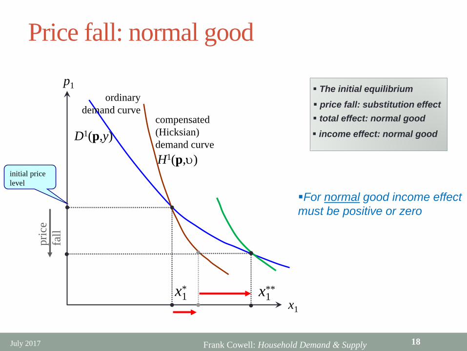
Price fall: normal good

compensated (Hicksian) demand curve

pric

e fa

ll

x1

p1

H1(p,υ)

*x1

The initial equilibrium price fall: substitution effect total effect: normal good

initial price level

For normal good income effect must be positive or zero

ordinary demand curve

x1**

income effect: normal goodD1(p,y)

July 2017 18


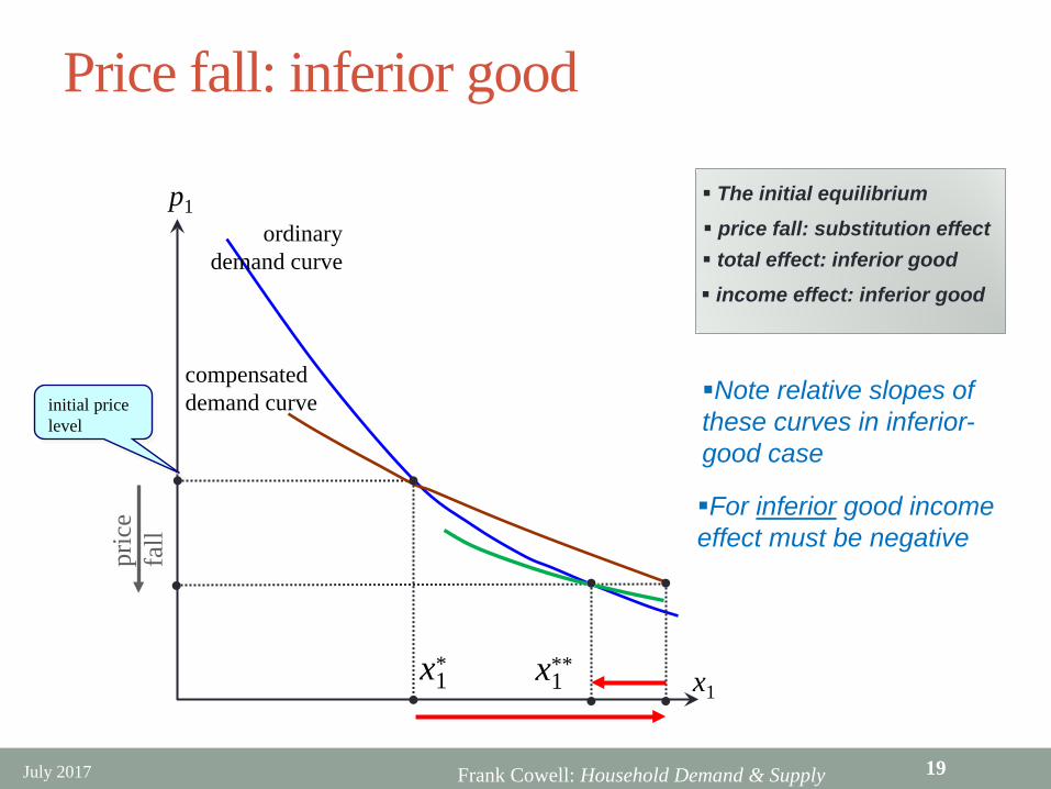
Price fall: inferior good

compensated demand curve

pric

e fa

ll

x1

p1

*x1

The initial equilibrium price fall: substitution effect total effect: inferior good

initial price level

For inferior good income effect must be negative

ordinary demand curve

x1**

income effect: inferior good

Note relative slopes of these curves in inferior-good case

July 2017 19


Features of demand functionsHomogeneous of degree zero Satisfy the “adding-up” constraint Symmetric substitution effectsNegative own-price substitution effects Income effects could be positive or negative:

• in fact they are nearly always a pain

July 2017 20


Overview

Response functions

Slutskyequation

Supply of factors

Examples


Extending the Slutsky analysis

July 2017 21


Consumer demand: alternative approachNow for an alternative way of modelling consumer responses Take a type-2 budget constraint

• endogenous income• determined by value of resources you own

Analyse the effect of price changes• will get usual income and substation effect• but an additional effect• arises from the impact of price on the valuation of income

July 2017 22


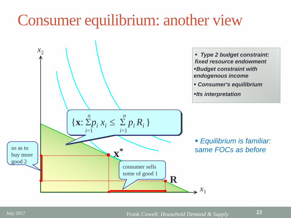
Consumer equilibrium: another view

Rx1

x2

x*

Type 2 budget constraint: fixed resource endowmentBudget constraint with endogenous income Consumer's equilibriumIts interpretation

Equilibrium is familiar: same FOCs as before

n n{x: Σpi xi ≤ Σ pi Ri }

i=1 i=1

so as to buy more good 2

consumer sells some of good 1

July 2017 23


Two useful concepts

From the analysis of the endogenous-income case derive two other tools:

1. The offer curve:• Path of equilibrium bundles mapped out by prices• Depends on “pivot point” - the endowment vector R

2. The household’s supply curve: • The “mirror image” of household demand • Again the role of R is crucial

July 2017 24


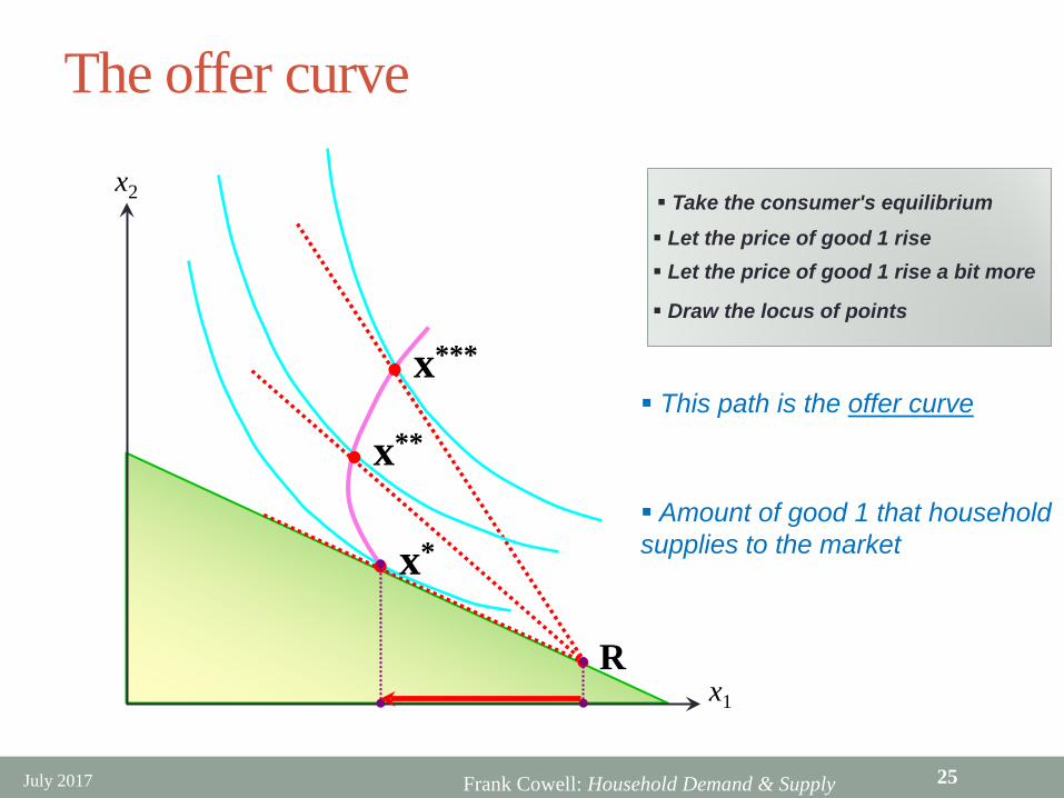
The offer curve

Rx1

x2

x*

x***

x**

Take the consumer's equilibrium Let the price of good 1 rise Let the price of good 1 rise a bit more

Draw the locus of points

This path is the offer curve

Amount of good 1 that household supplies to the market

July 2017 25


supply of good 1

p1

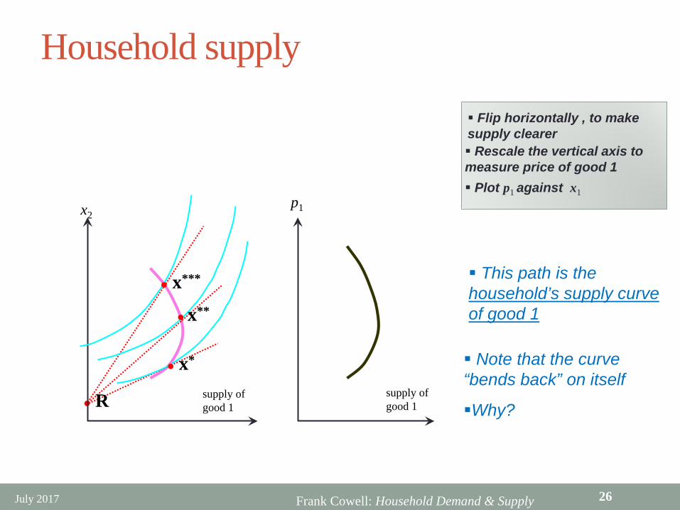
Household supply

Flip horizontally , to make supply clearer Rescale the vertical axis to measure price of good 1 Plot p1 against x1

This path is the household’s supply curve of good 1

R supply of good 1

x2

x*

x***

x**

Note that the curve “bends back” on itself

Why?

July 2017 26


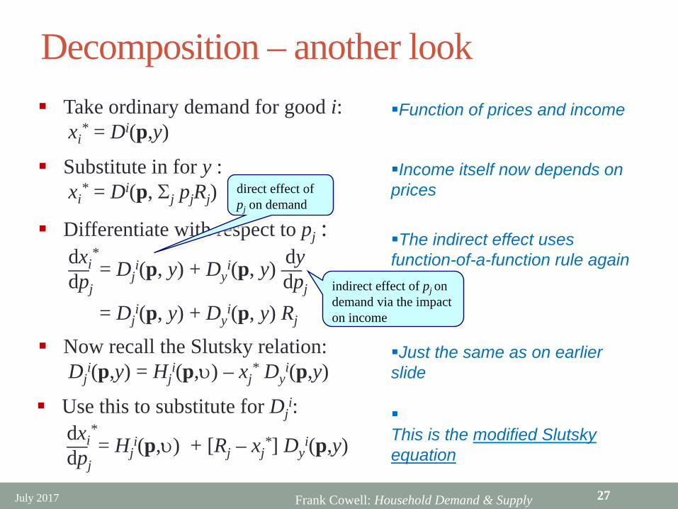
Decomposition – another lookFunction of prices and income

Differentiate with respect to pj : dxi

* dy— = Dji(p, y) + Dy

i(p, y) —dpj dpj

= Dji(p, y) + Dy

i(p, y) Rj

Income itself now depends on prices

Now recall the Slutsky relation: Dj

i(p,y) = Hji(p,υ) – xj

* Dyi(p,y)

The indirect effect uses function-of-a-function rule again

Just the same as on earlier slide

Use this to substitute for Dji:

dxi*

— = Hji(p,υ) + [Rj – xj

*] Dyi(p,y)dpj

This is the modified Slutskyequation

Take ordinary demand for good i:xi

* = Di(p,y)

Substitute in for y :xi

* = Di(p, Σj pjRj) direct effect of pj on demand

indirect effect of pj on demand via the impact on income

July 2017 27


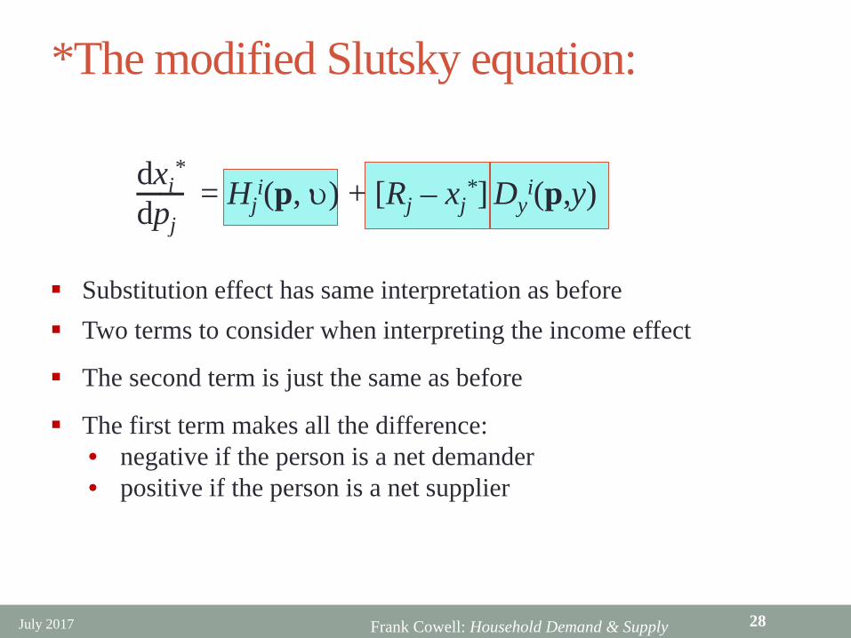
*The modified Slutsky equation:

Substitution effect has same interpretation as before Two terms to consider when interpreting the income effect

The second term is just the same as before

The first term makes all the difference:• negative if the person is a net demander• positive if the person is a net supplier

dxi*

── = Hji(p, υ) + [Rj – xj

*] Dyi(p,y)dpj

July 2017 28


Overview

Response functions

Slutskyequation

Supply of factors

Examples


Labour supply, savings…

July 2017 29


Some examplesMany important economic issues fit this type of model :

• Subsistence farming• Saving• Labour supply

It's important to identify the components of the model• How are the goods to be interpreted?• How are prices to be interpreted?• What fixes the resource endowment?

To see how key questions can be addressed• How does the agent respond to a price change?• Does this depend on the type of resource endowment?

July 2017 30


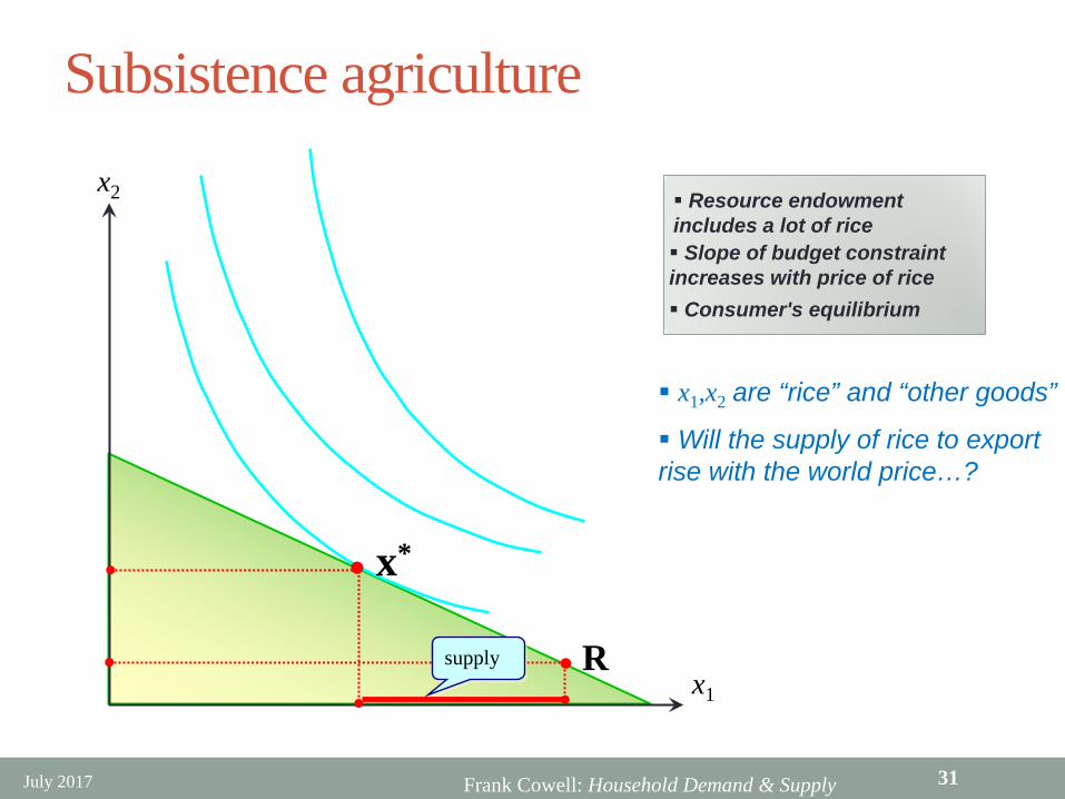
Subsistence agriculture

Rx1

x2

x*

Resource endowment includes a lot of rice Slope of budget constraint increases with price of rice Consumer's equilibrium

supply

Will the supply of rice to export rise with the world price…?

x1,x2 are “rice” and “other goods”

July 2017 31


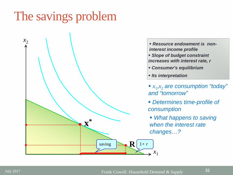
The savings problem

Rx1

x2

x*

Resource endowment is non-interest income profile Slope of budget constraint increases with interest rate, r Consumer's equilibrium Its interpretation

Determines time-profile of consumption

saving 1+ r

What happens to saving when the interest rate changes…?

x1,x2 are consumption “today” and “tomorrow”

July 2017 32


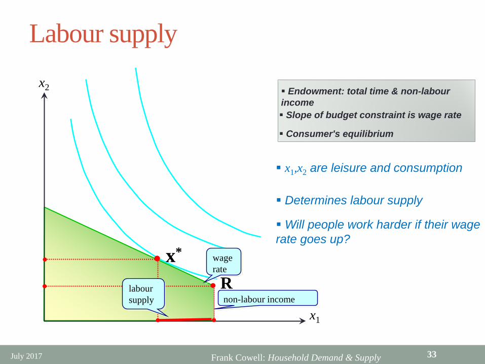
Labour supply

R

x1

x2

x*

Endowment: total time & non-labour income Slope of budget constraint is wage rate

Consumer's equilibrium

Determines labour supply

labour supply

wage rate

Will people work harder if their wage rate goes up?

x1,x2 are leisure and consumption

non-labour income

July 2017 33


Modified Slutsky: labour supply

Let ℓ:=[Ri – xi*] be the supply of labour

and s the share of earnings in total income y, Then we get: dxi

*— = Hi

i(p,υ) + ℓ Diy(p,y)dpi

The general form. We are going to make a further simplifying assumption

Rearranging :pi dxi

* pi y– — — = – — Hii(p,υ) – s — Di

y(p,y)ℓ dpi ℓ ℓ

Suppose good i is labour time; then Ri – xi is the labour you sell in the market (leisure time not consumed); pi is the wage rate

Divide by labour supply; multiply by (-) wage rate

Write as elasticities of labour supply:εtotal = εsubst + s εincome

The Modified Slutsky equation in a simple form

Take the modified Slutsky:dxi

*— = Hi

i(p,υ) + [Ri – xi*] Di

y(p,y)dpi

.

.

July 2017 34


SummaryHow it all fits together:

Compensated (H) and ordinary (D) demand functions can be hooked together. Slutsky equation breaks down effect of price i on demand for j Endogenous income introduces a new twist when prices change

July 2017 35


What next? The welfare of the consumerHow to aggregate consumer behaviour in the market

July 2017 36

Household Demand and Supply - London School of...

Documents

Transcript of Household Demand and Supply - London School of...