
HOUSEHOLD DEBT AND BUSINESS CYCLES WORLDWIDE Atif R. … · Atif R. Mian, Amir Sufi, and Emil...
64
NBER WORKING PAPER SERIES HOUSEHOLD DEBT AND BUSINESS CYCLES WORLDWIDE Atif R. Mian Amir Sufi Emil Verner Working Paper 21581 http://www.nber.org/papers/w21581 NATIONAL BUREAU OF ECONOMIC RESEARCH 1050 Massachusetts Avenue Cambridge, MA 02138 September 2015 This research was supported by funding from the Initiative on Global Markets at Chicago Booth, the Fama-Miller Center at Chicago Booth, and Princeton University. We thank Giovanni Dell'Ariccia, Andy Haldane, Óscar Jordá, Anil Kashyap, Guido Lorenzoni, Virgiliu Midrigan, Emi Nakamura, Jonathan Parker, Chris Sims, Andrei Shleifer, Paolo Surico, Alan Taylor, and seminar participants at Princeton University, Northwestern University, Harvard University, NYU, NYU Abu Dhabi, UCLA, the Swedish Riksbank conference on macro-prudential regulation, Danmarks Nationalbank, the Central Bank of the Republic of Turkey, Wharton, the Bank of England, the Nova School of Business and Economics, the NBER Monetary Economics meeting, and the NBER Lessons from the Crisis for Macroeconomics meeting for helpful comments. Elessar Chen and Seongjin Park provided excellent research assistance. The views expressed herein are those of the authors and do not necessarily reflect the views of the National Bureau of Economic Research. NBER working papers are circulated for discussion and comment purposes. They have not been peer-reviewed or been subject to the review by the NBER Board of Directors that accompanies official NBER publications. © 2015 by Atif R. Mian, Amir Sufi, and Emil Verner. All rights reserved. Short sections of text, not to exceed two paragraphs, may be quoted without explicit permission provided that full credit, including © notice, is given to the source.
Transcript of HOUSEHOLD DEBT AND BUSINESS CYCLES WORLDWIDE Atif R. … · Atif R. Mian, Amir Sufi, and Emil...

NBER WORKING PAPER SERIES
HOUSEHOLD DEBT AND BUSINESS CYCLES WORLDWIDE
Atif R. MianAmir Sufi
Emil Verner
Working Paper 21581http://www.nber.org/papers/w21581
NATIONAL BUREAU OF ECONOMIC RESEARCH1050 Massachusetts Avenue
Cambridge, MA 02138September 2015
This research was supported by funding from the Initiative on Global Markets at Chicago Booth, the Fama-Miller Center at Chicago Booth, and Princeton University. We thank Giovanni Dell'Ariccia, Andy Haldane, Óscar Jordá, Anil Kashyap, Guido Lorenzoni, Virgiliu Midrigan, Emi Nakamura, Jonathan Parker, Chris Sims, Andrei Shleifer, Paolo Surico, Alan Taylor, and seminar participants at Princeton University, Northwestern University, Harvard University, NYU, NYU Abu Dhabi, UCLA, the Swedish Riksbank conference on macro-prudential regulation, Danmarks Nationalbank, the Central Bank of the Republic of Turkey, Wharton, the Bank of England, the Nova School of Business and Economics, the NBER Monetary Economics meeting, and the NBER Lessons from the Crisis for Macroeconomics meeting for helpful comments. Elessar Chen and Seongjin Park provided excellent research assistance. The views expressed herein are those of the authors and do not necessarily reflect the views of the National Bureau of Economic Research.
NBER working papers are circulated for discussion and comment purposes. They have not been peer-reviewed or been subject to the review by the NBER Board of Directors that accompanies official NBER publications.
© 2015 by Atif R. Mian, Amir Sufi, and Emil Verner. All rights reserved. Short sections of text, not to exceed two paragraphs, may be quoted without explicit permission provided that full credit, including © notice, is given to the source.

Household Debt and Business Cycles Worldwide Atif R. Mian, Amir Sufi, and Emil Verner NBER Working Paper No. 21581September 2015, Revised July 2016JEL No. E17,E2,E21,E32,E44,G01,G21
ABSTRACT
An increase in the household debt to GDP ratio in the medium run predicts lower subsequent GDP growth, higher unemployment, and negative growth forecasting errors in a panel of 30 countries from 1960 to 2012. Consistent with the “credit supply hypothesis,” we show that low mortgage spreads predict an increase in the household debt to GDP ratio and a decline in subsequent GDP growth when used as an instrument. The negative relation between the change in household debt to GDP and subsequent output growth is stronger for countries that face stricter monetary policy constraints as measured by a less flexible exchange rate regime, proximity to the zero lower bound, or more external borrowing. A rise in the household debt to GDP ratio is contemporaneously associated with a consumption boom followed by a reversal in the trade deficit as imports collapse. We also uncover a global household debt cycle that partly predicts the severity of the global growth slowdown after 2007. Countries with a household debt cycle more correlated with the global household debt cycle experience a sharper decline in growth after an increase in domestic household debt.
Atif R. MianPrinceton UniversityBendheim Center For Finance26 Prospect AvenuePrinceton, NJ 08540and [email protected]
Amir SufiUniversity of ChicagoBooth School of Business5807 South Woodlawn AvenueChicago, IL 60637and [email protected]
Emil VernerPrinceton UniversityBendheim Center For Finance26 Prospect AvenuePrinceton, NJ [email protected]
The Great Recession has sparked new questions about the relation between household debt and
the macroeconomy. Recent theoretical and empirical research recognizes that a sudden and large
increase in household debt could lower subsequent output growth in the presence of monetary and
fiscal policy constraints. Moreover, households may not internalize the macroeconomic effects of
their own borrowing, making the economy susceptible to “excessive” credit growth.1
However, empirical evidence on increases in household debt and subsequent economic perfor-
mance is largely limited to the United States and the most recent global recession. A more system-
atic evaluation of the empirical relation between household debt and business cycles worldwide is
needed in order to understand if recent events are representative of a broader pattern. This is im-
portant given the dramatic rise in household debt to GDP ratios over the last 50 years documented
by Jorda et al. (2014a).
This paper compiles data for 30 countries from 1960 to 2012 and provides several new results
that highlight the importance of household credit shocks in driving business cycles worldwide.
There are two broad hypotheses that relate household debt to business cycles. The “credit de-
mand hypothesis” posits a positive relationship between current household borrowing and future
income. Household borrowing in this view is driven by productivity or technology shocks that
increase expected future income, spurring higher consumption and borrowing in anticipation. On
the other hand, the “credit supply hypothesis” holds that higher household borrowing is driven by
an expansion in the availability of credit. If there are plausible frictions such as nominal rigidities
or monetary policy constraints, then households may borrow excessively which leads to an eventual
slowdown in GDP growth.
Distinguishing the credit demand and credit supply hypotheses is important for our under-
standing of economic fluctuations and for guiding policy. For example, the relation between house-
hold debt and the business cycle is spuriously generated by expected income shocks in the credit
demand hypothesis, leaving no special role for regulation. However, under the credit supply hy-
pothesis, households may over-extend themselves when borrowing during a credit supply boom,
necessitating the need for macro-prudential regulation.
We present a number of results that reject the credit demand hypothesis and support the credit
1See, e.g., Mian and Sufi (2014) and IMF (2012) for empirical evidence and Eggertsson and Krugman (2012), Guerrieriand Lorenzoni (2015), Farhi and Werning (2015), Korinek and Simsek (2016), Schmitt-Grohe and Uribe (2016), andMartin and Philippon (2014) for theoretical analysis.
1
supply hypothesis. We show that an increase in the household debt to GDP ratio over a three
year period2 in a given country predicts subsequently lower output growth.3 The magnitude of the
predictive relation is large – a one standard deviation increase in the household debt to GDP ratio
over the last 3 years (6.2 percentage points) is associated with a 2.1 percentage point decline in
GDP over the next three years. This relation is robust across time and space. The strong negative
relation between changes in household debt and subsequent income growth is unique to household
debt. There is no such relation for non-financial firm debt.
The slowdown in GDP in response to an increase in household debt to GDP is not anticipated
by professional forecasters at the IMF and OECD. Consequently, an increase in the household
debt to GDP ratio from four years ago to last year predicts negative GDP growth forecast errors
from this year to three years forward. This finding suggests that the negative correlation between
household debt booms and subsequently lower output growth is unlikely to be driven by news or
income shocks seen by agents in the economy but unobservable to us as econometricians.
We also put together a new cross-country panel series on mortgage credit spreads to show
that low credit spreads predict an increase in household debt to GDP. If an increase in household
debt were driven by credit demand shocks, then we would expect the opposite relation. Using
the mortgage spread as an “imperfect instrument” in the spirit of Nevo and Rosen (2012), we
set-identify the negative effect of a credit supply-induced increase in household debt on subsequent
GDP growth.
The credit supply hypothesis also predicts that the negative relation between the change in
household debt and subsequent GDP growth is stronger when certain constraints on adjustment
are present, such as restrictions on monetary policy. We find that this is indeed the case in the
data. The negative relation between the change in household debt and subsequent GDP growth
is stronger under more rigid exchange rate regimes, or when a country is close to the zero lower
bound on nominal interest rates, or when a country borrows from abroad. Similarly, an increase in
the household debt to GDP ratio predicts an increase in the future unemployment rate, showing
2As we explain below, the three year period is not chosen ad hoc. It is based on what the data tell us about thelength of credit cycles.
3We follow standard time-series econometrics semantics and use the term “predict” to refer to the predicted value ofan outcome using the entire sample used to estimate the regression. This is in contrast to the term “forecast” thatrefers to the estimated value of the outcome variable for an observation that is not in the sample used to estimatethe regression coefficients. See Stock and Watson (2011), chapter 14.
2
evidence of underutilization of resources. Further, consistent with the credit supply hypothesis,
the expansion in debt is used to fuel consumption as opposed to investment. The trade balance
deteriorates, and the consumption share of imports rises sharply.
We explore the global dimension of the household debt cycle by first showing that a rise in
household debt to GDP leads to a subsequent reduction in the trade deficit as imports decline.
The resulting increase in net exports partially offsets the large negative effect of the household debt
boom on consumption and investment, and it points to the importance of external spillovers to
other countries.
We find that countries with a household debt to GDP cycle that is more strongly correlated with
the global debt cycle see a stronger decline in future output growth after a rise in the household
debt to GDP ratio. This is driven by the inability of countries to boost net exports when many
countries are suffering from a household debt hangover at the same time. Trade linkages lead to a
global debt cycle: there is a stronger negative relation between the rise in global household debt to
GDP and subsequent global growth.
The relation between a rise in global household debt and subsequent slowdown in global GDP
growth is not driven by the post-2000 period alone. In fact, using estimates from only pre-2000
data, we show that our regression model forecasts (out-of-sample) quite accurately the slowdown
in global growth during the late 2000s given the dramatic rise in global household debt during the
mid-2000s.
Our paper follows the recent influential work by Jorda et al. (2014a), Schularick and Taylor
(2012), Jorda et al. (2013), and Jorda et al. (2014b) on the role of private debt in the macroe-
conomy. The authors put together long-run historical data for advanced economies to show that
credit growth, especially mortgage credit growth, predicts financial crises (also see Dell’Ariccia
et al. (2012)). Moreover, conditional on having a recession, stronger credit growth predicts deeper
recessions.4
4There is also cross-sectional evidence from the recent recession in the United States and Europe (see, e.g., Mianand Sufi (2014), Glick and Lansing (2010), and IMF (2012)) showing that areas with the largest rise in householddebt during the boom saw the biggest decline in economic activity during the bust. Baron and Xiong (2016) showthat a large increase in bank credit to GDP predicts lower equity returns, and Cecchetti and Kharroubi (2015)find that the growth in the financial sector is correlated with lower productivity growth. Cecchetti et al. (2011)estimate country-level panel regressions relating economic growth from t to t + 5 to the level of government, firm,and household debt in year t. They do not find strong evidence that the level of private debt predicts growth.Reinhart and Rogoff (2009) provides an excellent overview of the patterns of financial crises throughout history.
3
Our methodological point of departure from the above literature is that we focus on estimating
the unconditional relation between changes in household debt and subsequent GDP growth, while
earlier work focuses on the effect of increases in credit on recession severity conditional on having
a recession. Further, our analysis provides a number of results that should guide the nascent theo-
retical literature on private credit and business cycles. For example, our results on the asymmetry
between household debt and non-financial firm debt, predictability of labor market slackness, as
well as predictability of GDP forecast errors help rule out spurious factors that could produce a
relation between changes in household debt and subsequent GDP growth. Our findings regard-
ing the consumption boom, heterogeneity with respect to monetary regimes, and the influence of
credit supply shocks on household debt changes are important for understanding the mechanisms
that generate the negative relation between household debt changes and subsequent GDP growth.
Finally, our results on the external margin spillovers highlight the importance of the “global house-
hold debt cycle,” which was also an important precursor to the most recent global recession. We
believe all of these results are novel to the literature.
While the existing literature in macro-finance has made important contributions in understand-
ing the “investment” channel for business cycle dynamics (see e.g., Bernanke and Gertler (1989),
Kiyotaki and Moore (1997), Caballero and Krishnamurthy (2003), Brunnermeier and Sannikov
(2014) and Lorenzoni (2008)), our results highlight the importance of a debt-driven “consumption”
channel for business cycle dynamics. We hope our results will help guide the burgeoning theoret-
ical literature in this area, such as Eggertsson and Krugman (2012), Farhi and Werning (2015),
Guerrieri and Lorenzoni (2015), Korinek and Simsek (2016), Martin and Philippon (2014), and
Schmitt-Grohe and Uribe (2016).5
The remainder of the paper is structured as follows. The next section presents the data and
summary statistics. Section 2 presents the empirical specification. Sections 3 and 4 provide empir-
ical estimates of the relation between household debt changes, output growth and GDP forecasts.
Section 5 presents evidence on heterogeneity with respect to monetary policy frictions, and section
5While we have restricted our attention here to models where over-borrowing is driven by an externality, we donot argue that behavioral biases are unimportant. For example, households may overborrow due to hyperbolicpreferences as in Laibson (1997) or a“neglected risk” as in Gennaioli et al. (2012). Such excessive borrowing canthen lead to a slowdown in output growth, as in Barro (1999). Further, we do not take a stand on what drives thevariation in credit supply, which could be driven by behavioral biases such as sentiment shifts. We do, however,believe that debt is an important part of the story. We discuss this point further in the conclusion.
4
6 considers alternative hypotheses. Section 7 presents evidence on the global household debt cycle,
and section 8 concludes.
1 Data and Summary Statistics
1.1 Data
We build a country-level unbalanced panel dataset that includes information on household and non-
financial firm debt to GDP, national accounts, unemployment, professional GDP forecasts, credit
spreads, and international trade. The countries in the sample and the years covered are summarized
in Table 1. The data are annual and range from 1960 to 2012, providing over 900 country-years.
Details on variable definitions and data sources are provided in the online data appendix. Here we
briefly describe the key variables measuring expansions in household and non-financial firm debt.
We measure the level of household and non-financial firm debt as household debt to GDP
ratio and non-financial firm debt to GDP ratio respectively. Likewise, we measure the change
in household and firm debt from year t − k to year t as ∆k(HHD/Y )t and ∆k(FD/Y )t, where
HHD and FD are the outstanding levels of credit to households and non-financial corporations,
respectively. Credit is defined as loans and debt securities financed by domestic and foreign banks,
as well as non-bank financial institutions. Outstanding credit to households and non-financial
corporations are from the Bank for International Settlement’s (BIS) “Long series on credit to the
private non-financial sector” database. Household and firm debt together constitute total credit to
the private sector in a country.6
1.2 Summary Statistics
Table 2 displays summary statistics for the change in total private, household, and non-financial
firm debt to GDP, as well as the other variables.7 Our empirical analysis uses both the level of debt
to GDP in panel vector autoregressions (VARs) and changes over three years in a single equation
6The series on credit to households and non-financial firms are available for 34 countries. We exclude China, India,and South Africa, as the decomposed credit series only start in 2006 for China and South Africa and 2007 forIndia. We also exclude Luxembourg, as the data on non-financial firm credit for Luxembourg is highly volatile, withchanges of similar magnitude as annual GDP in some years.
7With the exception of the serial correlation, all statistics are computed by pooling observations from all countries.The serial correlation is a weighted average of the serial correlations for each country, with the underlying numberof observations for each country as weights.
5
estimation framework. Table 2 shows that total private sector debt to GDP, PD/Y , has been
increasing by 3.11 percentage points per year on average, with household debt to GDP increasing
slightly more quickly than non-financial firm debt. The change in non-financial firm debt is about
two times as volatile as household debt, and both series are reasonably persistent. Other patterns
documented in Table 2 are consistent with the small open economy business cycle literature. Total
consumption expenditure is approximately as volatile as output, while durable consumption and
investment are about 2.8 and 3.6 times as volatile as output, respectively. Imports and exports are
roughly four times more volatile than output.
2 Conceptual Framework and Empirical Methodology
Our empirical analysis centers on estimating the predictive relation between the expansion in house-
hold debt and subsequent GDP growth. For a given country, let ∆hyt+h measure the change in
the logarithm of real GDP from year t to t + h, and let ∆kdHHt refer to a change in a measure of
household debt from t− k to the end of t. Our empirical specification in its simplest form can be
written as:
∆hyt+h = αh + βhHH∆kdHHt + εt+h. (1)
Estimating (1) for increasing values of h traces out the Jorda (2005) local projection impulse
response function {βhHH} for the change in household debt on subsequent growth.
Since household debt expansion and future GDP growth are endogenous variables, an estimate
of βhHH cannot be interpreted as a causal or structural relation at face value. In this section we
highlight two different classes of theories regarding the fundamental shocks that drive the correlation
between changes in debt and subsequent output growth. We refer to these as “credit demand” and
“credit supply” hypotheses, respectively. We then specify our empirical methodology to separate
these two hypotheses.
6

2.1 The Credit Demand Hypothesis
A natural reason for household debt to expand today is in anticipation of higher income tomor-
row, as in the standard permanent income hypothesis. We refer to this as the “credit demand
hypothesis.” The anticipation of higher income tomorrow could be driven by shocks ranging from
technology shocks to natural resource discovery and terms of trade shocks. A technological shock
may raise future output directly through higher productivity, or indirectly by relaxing borrowing
constraints through financial innovation. Justiniano et al. (2015) model shocks to credit demand
in this manner. Another related example would be a self-reinforcing “rational bubble” shock as in
Martin and Ventura (2012) that raises agents’ borrowing capacity today and translates into higher
output tomorrow.
Abstracting away from the deeper source of higher output tomorrow, consider a small open
economy with exogenously given output and a continuum of infinitely lived households. Output
yt follows a stochastic process with ψt+jt = Et∆yt+j representing the expected change in income j
periods forward at time t. Households face no borrowing constraints and maximize,
E0
∞∑t=0
βtu(ct).
There is a risk-free one period bond that can be traded internationally with each household facing
a sequential budget constraint,
ct + (1 + r)dt−1 = yt + dt, (2)
and a no-Ponzi game constraint,
limj→∞
Etdt+j
(1 + r)j= 0. (3)
The Euler equation of this problem can be written as u′(ct) = β(1 + r)Etu′(ct+1). Assuming
β(1 + r) = 1 and quadratic utility with U(c) = −12(c − c)2 with c ≤ c, makes marginal utility
linear and hence consumption a random walk with ct = Etct+1. Iterating forward (2) and using (3)
and ct = Etct+1, we get that consumption equals expected permanent income Etypt minus interest
7

payments on outstanding debt rdt−1 in equilibrium,
ct = Etypt − rdt−1 =
r
(1 + r)Et
∞∑j=0
yt+j(1 + r)j
− rdt−1. (4)
Plugging ct = Etypt − rdt−1 into equation (2), we can write down the change in debt at time t in
terms of the present value of expected changes in future income:
∆dt =
∞∑j=1
ψt+jt
(1 + r)j. (5)
Growth in debt is driven by higher demand for credit in response to expected future income
growth and a desire to smooth consumption.8 Since credit supply is considered fixed in this thought
experiment, as long as the credit supply schedule is upward sloping we get the additional prediction
that credit growth is associated with rising spreads as in Justiniano et al. (2015).
To summarize the “credit demand hypothesis”: household credit expansions driven by credit
demand shocks predict stronger future output growth and (weakly) higher interest rates on household
credit.
2.2 The Credit Supply Hypothesis
An alternative interpretation of credit expansions is that they are driven by credit supply shocks.
A credit supply shock represents relaxation in lending constraints. For a given interest rate and
potential borrower, lenders are willing to lend more or on cheaper terms. Lenders may expand the
supply of available credit due to the adoption of a securitization technology as in Justiniano et al.
(2015). Alternatively supply may expand because of increased demand for saving, an exogenous
decline in the risk spread as in Schmitt-Grohe and Uribe (2016), or a decline in the risk spread due
to “diagnostic expectations” as in Bordalo et al. (2015).
If household debt expands because of credit supply shocks, then the implications are different
from those of the credit demand hypothesis outlined above. First, an increase in the supply of credit
8Strictly speaking, the debt in this small open economy model represents net foreign debt. This is due to theassumption of a representative agent. More broadly, one could introduce heterogeneity where some agents withina country receive a positive productivity shock and borrow from other agents in the same economy. Our empiricalsection uses total gross private debt, whether borrowed domestically or from abroad. But we also show results fornet foreign debt.
8
will be associated with a decline in credit spreads as opposed to an increase. Second, a credit supply
shock can potentially break the positive association between credit growth today and subsequent
output growth. The association may even become negative, following the intuition in Eggertsson
and Krugman (2012), Korinek and Simsek (2016), and Schmitt-Grohe and Uribe (2016).
There are two key ingredients needed to generate a negative correlation between credit-supply-
induced household debt growth and subsequent output growth. The first ingredient is the presence
of certain frictions, such as the zero lower bound (ZLB) on nominal interest rates that translates
a high level of household indebtedness into lower GDP in response to a financial shock. Second,
there is an externality in that households fail to fully internalize the potentially negative macroeco-
nomic consequences of their individual borrowing decisions. The result is that there is “excessive”
household borrowing in response to credit supply expansion, resulting in predictably lower GDP
going forward.
Formally, consider the same representative agent set up as above, except that there are only
two periods, t and t + 1. The output capacity of the economy is fixed at y, with yt = y. The
economy is hit by a financial shock at the beginning of t+ 1, and its response to the shock depends
on the overall level of debt that households borrowed in period t, Dt, and the extent of “frictions”,
Φ, present in the economy. In particular,
yt+1 =
y if Dt ≤ D
y − f(DtD,Φ) with f(1, .) = 0, f1 > 0 and f12 > 0, otherwise.
(6)
Equation (6) implies that if households choose to take on “excessive” debt (Dt > D) in period t,
then the economy cannot operate at full capacity in period t+1. The output shortfall will be larger
for higher levels of household debt and more severe macroeconomic frictions (i.e. higher Φ).
Equation (6) can be motivated by Schmitt-Grohe and Uribe (2016), among others. The friction,
Φ, in their model is a combination of downward wage rigidity and a monetary policy constraint due
to a fixed exchange rate. The financial shock in their model is the reversal of a temporary interest
rate decline, which causes domestic demand for non-tradables to fall. However, the combination of
downward wage rigidity and restricted monetary policy prevents the economy from adjusting fully,
resulting in unemployment and decline in output.
9
A related but separate rationale for (6) is provided by Eggertsson and Krugman (2012) and
Korinek and Simsek (2016). These are closed economy models where the financial shock is a
tightening of borrowing constraint faced by the impatient consumer. The authors show that if debt
levels are sufficiently high, the deleveraging shock will tip the economy into a zero lower bound
constraint and recession.9
While the financial shock in both Schmitt-Grohe and Uribe (2016) and Korinek and Simsek
(2016) is fully anticipated, households do not internalize the negative macroeconomic consequences
of their borrowing due to an externality. The result is that there is “excessive” borrowing ex-ante
if households are given a chance to borrow due to an expansionary credit supply shock.
We can see this formally by closing the model and solving for the level of debt chosen by
consumers in period t. For simplicity, assume that the economy enters t with no debt at all, and
there is a credit supply shock at the beginning of the period that enables households to borrow.
There is a continuum of identical households of measure one. Each household chooses consumption
ct, ct+1, and debt dt to maximize utility u(ct)+βu(ct+1), subject to budget constraints yt = ct− dt1+rt
and yt+1(Dt) = ct+1 + dt.
Since there is measure one of total households, dt = Dt in equilibrium. However, each household
will choose dt, taking as given their equilibrium expectation of Dt. This observation gives rise to
a “demand externality” in the model: households do not internalize the fact that their choice of
debt could lead to lower output next period, leading to excessive borrowing relative to the social
optimum.
The demand externality becomes transparent by comparing the private Euler equation of each
household, in which a household takes Dt as given, with the social planner’s Euler equation who
internalizes the effect of her choice of dt on Dt. The private Euler equation is u′(ct)u′(ct+1) = β(1 + rt),
while the social Euler equation is u′(ct)u′(ct+1) = β(1+rt)(1+f1D
−1). Thus private consumption ct (and
hence borrowing dt) is too high in the decentralized equilibrium relative to the social optimum.
Assuming log utility, households take on debt, dt = 11+β (yt+1(Dt) − β(1 + rt)y).10 If the
9There are other papers in the macro-finance literature that share some of the features detailed here, includingJustiniano et al. (2015), Favilukis et al. (2015)), Martin and Philippon (2014), and Guerrieri and Lorenzoni (2015).There are additional models based on pecuniary or fire sales externalities that focus on the potential for excessiveleverage among non-financial firms. Examples include Shleifer and Vishny (1992), Kiyotaki and Moore (1997),Lorenzoni (2008), and Davila (2015). Pecuniary externalities can also amplify the effect of household debt, especiallyfor collateralized borrowing such as mortgages.
10We assume D < y(1−β)1+β
, which guarantees that there exists a low enough rt that generates an output slump in
10
borrowing rate rt is low enough (a correlate of the strength of the credit supply shock as in Schmitt-
Grohe and Uribe (2016)) then Dt > D, and the economy dips into a recession next period. While
the model here emphasizes a demand externality to rationalize excessive borrowing ex-ante, an
alternative rationale would be psychological factors such as the “diagnostic expectations” in Bordalo
et al. (2015) that lead people to neglect the future correction.
To summarize the “credit supply hypothesis”: An expansion in household debt driven by a
credit supply shock is associated with a decline in credit spreads on loans to households. There is
“excessive” borrowing ex-ante and a sufficiently large expansion in household debt predicts lower
subsequent output growth. This relationship is stronger when frictions such as monetary policy
constraints are present.
2.3 Empirical Methodology and Identification
This section develops the empirical methodology that allows us to understand the extent to which
credit demand versus credit supply shocks drive household credit and business cycles. Our method-
ology exploits the three predictions where the two hypotheses differ: (i) the correlation of changes
in debt with credit spreads, (ii) the correlation of changes in debt and subsequent output growth,
and (iii) the dependence of the correlation in (ii) on the presence of frictions.
We augment equation (1) to allow for multiple countries in a panel setting and a richer set
of controls variables as is typical in the local projection method (Jorda (2005)). Let yit be the
dependent variable of interest, such as log real GDP. We estimate the IRF for an innovation in
debt using:
∆hyit+h = αhi + βhHH∆3dHHit−1 + βhF∆3d
Fit−1 +X ′i,t−1Γh + εhit, (7)
where αi are country fixed effects, ∆3 refers to the difference over three years, i.e., ∆3dHHit =
(dHHit − dHHit−3), dHHit and dFit correspond to the household debt to GDP ratio and the non-financial
firm debt to GDP ratio, respectively, and h = 1, 2, ... is the forecast horizon. The vector Xit
includes additional control variables such as several lags in the dependent variable in the spirit of
the local projection method. The coefficients βhHH and βhF trace out the IRF for y of a change in
period t+ 1.
11
household and non-financial firm debt, respectively. Initially, we do not include year fixed effects:
we introduce these in the Section 7 in the context of the global credit cycle.
We difference the right-hand-side debt to GDP ratios over a three year period. This is motivated
by the VAR analysis in Figure 7(a) below which shows that a shock to the household debt to GDP
ratio persists for a three to four year period before dissipating. We also lag right hand side variables
by one year to ensure that variables on the right hand side are observable at time t by forecasters.
Appendix Table A1 shows that our results are not sensitive to either of these exact choices.
It is important to normalize debt so that dHHit and dFit refer to debt normalized by the size of
the economy. In theory, it is the growth of debt relative to the size of the economy that matters.
The danger in not normalizing debt is that episodes of large real debt growth from a small base
can appear large without being economically meaningful.
We use two different normalization methods. The first method normalizes debt by GDP, with
dHHit = HHDitYit
and dFit = FDitYit
, where HHD and FD refer to nominal household debt and non-
financial firm debt respectively, and Y refers to nominal GDP. A potential drawback of this nor-
malization is that the change in debt to GDP variable also captures innovations to GDP, and not
just debt. We therefore also adopt a second normalization method, where the change in debt is
computed relative to a fixed base year GDP, i.e., ∆3dHHit = HHDit−HHDit−3
Yit−3. Our empirical results
are similar regardless of the normalization method used.
The single equation local projections (LP) method offers certain advantages. First, it is flexible
in that it does not constrain the shape of the IRF between horizons h and h+1 (unlike a structural
vector auto regression, or SVAR). Second, it does not necessarily require that all variables enter all
equations simultaneously and therefore can provide a more parsimonius specification. Third, the LP
approach is flexible and allows for the estimation of state-dependent βhHH . For example, we can test
if the coefficient is stronger in fixed exchange rate regimes that face tight monetary constraints.11
Nonetheless, we also present results identifying a credit supply shock within a structural VAR.
Our key coefficient of interest in (7) is βhHH . Let ∆hyit+h and ∆3dHHit−1 be the residuals from a
11See Ramey and Zubairy (2014) as another example of estimating state-dependent impulse responses using localprojections.
12
regression on the other regressors (∆3dFit−1, X
′it−1), so that (7) can equivalently be written as,
∆hyit+h = αh + βhHH∆3dHHit−1 + uhit (8)
We are interested in isolating and identifying the effect of credit supply shocks on ∆hyit+h. The
identification problem is that ∆3dHHit−1 may be influenced by both credit supply and credit demand
shocks. The concern is that the error term uhit contains shocks to credit demand such as news of
higher future income, and ∆3dHHit−1 might be spuriously correlated with the error term. Formally,
the OLS coefficient in (8) can be written as,
βhOLS = βhHH +cov(∆3d
HHit−1, u
hit)
var(uhit). (9)
where βhHH is the true effect of credit supply shocks on future output. The key intuition from our
earlier discussion is that while the last covariance term is not observable, we can still sign this term
under the credit demand hypothesis: credit demand induces a positive correlation between future
income shocks and household credit growth today, socov(∆3dHHit−1,u
hit)
var(uhit)> 0. As a result, the OLS
estimate of the credit supply relation, βhHH , is biased upward. In other words, the credit supply
coefficient is set-identified with βhHH as the upper bound. This insight turns out to be useful in
our context since the OLS estimatation of (8) results in a strong and robust negative estimate for
βhHH .
This particular set-identification strategy comes under threat if cov(∆3dHHit−1, u
hit) < 0, so that
credit demand increases even though expected growth is lower going forward. This could be the
case if agents see a negative shock coming and borrow to hoard liquidity in anticipation. Several
of our results below contradict this alternative explanation for a negative correlation.
Identification of credit supply shocks in the OLS exploits the opposing predictions of credit
supply and credit demand hypotheses with regard to the correlation between household debt growth
and subsequent output growth. We can further adopt an “imperfect IV” approach in the spirit of
Nevo and Rosen (2012) by using the additional observation that while credit demand shocks are
associated with an increase in household credit spreads, credit supply shocks are associated with
lower spreads. This observation can be embedded in an “imperfect IV” framework to set-identify
13
the credit supply effect.
Let Zi,t−4 be the instrument that represents the household credit spread at the beginning of
the period when ∆3dHHit−1 is measured. Let σdz be the covariance between Zi,t−4 and ∆3d
HHit−1. If
the change in household debt is driven by credit supply shocks, then σdz < 0. We can test this in
the data, and if confirmed, σdz forms the “first stage” of our imperfect IV specification.12
Lower credit spreads are also unlikely to be associated with lower expected output growth. In
fact it is reasonable to assume that σuz ≤ 0, where σuz represents the covariance between the lagged
household credit spread and expected future output growth. Using Zi,t−4 as an instrument, the IV
coefficient in (8) is,
βhIV = βhHH +σuzσdz
(10)
Since the last term is weakly positive, βhIV provides an upper bound on the true credit supply effect,
which is once again set-identified. We shall adopt this IV methodology in both single equation and
VAR approaches.
We have so far focused on the identification of the coefficient βhHH . However, comparing the
estimated βhHH with βhF provides additional insights. As we will see, it turns out that there is
an important asymmetry in that βhHH is negative while βhF is close to zero. If estimated βhHH
were driven by spurious unobserved common shocks, such as productivity shocks, one would have
expected such spurious shocks to impact both the household debt and firm debt coefficients equally.
In other words, examining whether there are different correlations of household debt changes and
non-financial firm debt changes with subsequent growth can help “difference away” the effect of
these fundamental shocks.
While we have focused on the single equation local projections method here, the empirical
section also repeats the analysis within a VAR framework. We discuss these details in the empirical
section.
12An alternative instrument for credit supply shifts would be the share of total debt issuances by low credit qualitycorporations, as proposed in Greenwood and Hanson (2013). Their measure is only available for the United States.
14
3 Household Debt Expansions and Output Growth
3.1 Basic Result and Robustness
Table 3 presents estimates of equation (7) with output growth measured at a 3 year horizon, i.e.,
∆3yit+3. Column 1 sums household debt and non-financial firm debt and uses the overall change in
private debt to GDP on the right hand side. Columns 2 through 4 separate out the two components
of total private debt. There is a significant negative correlation between changes in private debt
and future output growth. Moreover, this negative correlation is entirely driven by the growth in
household debt (column 4). The magnitude of the negative correlation is large, with a one standard
deviation increase in the change in household debt to GDP ratio (6.2 percentage points) associated
with a 2.1 percentage point lower growth rate during the subsequent three years.
Figure 1 plots the coefficients from equation (7) to trace out the entire impulse response func-
tion. The negative relation between changes in private debt and subsequent output growth comes
exclusively from the rise in household debt. Moreover, the magnitude of the relation increases over
time. Expansions in household debt are associated with a protracted period of low output growth.
Figure 2 focuses on the three-year horizon and shows the scatter plot of Table 3, labeling each
country-year in our sample. There is a strong negative relation, and this relation is not driven
by outliers. Moreover, the relation is non-linear, a point which we return to in section 4. Ireland
and Greece during the Great Recession show up in the bottom right part of the scatter plot, but
several other episodes including Finland from 1989 to 1990 and Thailand during the East Asian
financial crisis also help explain the robust correlation. Panels b and c show the partial correlation
between future output growth and the change in household debt to GDP and non-financial firm
debt to GDP ratios, respectively. As already shown in column 4 of Table 3, the partial correlation
is negative for household debt, but flat for non-financial firm debt.
Column 5 of Table 3 includes lagged one-year GDP growth variables over the same period as
the change in debt, ∆yi,t−1, ∆yi,t−2 and ∆yi,t−3. The estimate of βhHH is robust to the inclusion
of lagged GDP growth controls, which shows that this result is not driven by some spurious mean
reversion in the output growth process.
Column 6 adds the change in government debt to GDP over the same period on the right hand
side. A rise in government debt to GDP is associated with moderately stronger growth over the
15
following three years, but the coefficient is small and not statistically significant.13 The negative
relation between future output growth over the medium run and past changes in debt to GDP
ratios is unique to household debt.
Is the negative overall estimate of β3HH representative of a broad set of countries, or only driven
by a select few? Figure 3 provides coefficients from estimating equation (7) separately for each
country. The coefficient on the household debt to GDP ratio is negative for twenty-four of the
thirty countries in our sample, and none of the country coefficients are significantly positive with
the exception of Turkey.14 The cross-country average of the estimates is -0.36 and the precision
weighted average is -0.40.
Table 4 provides some additional robustness checks on sample selection, standard errors, and
functional form of our debt variables. Columns 1 and 2 show that the βhHH estimate is larger in
absolute value for developed economies (-0.37), but the relation is also strong for emerging market
economies (-0.24). Columns 3 and 4 exclude the post-1990 period and the post-2000 period, showing
that the boom and bust cycle of the Great Recession of 2008 is not uniquely responsible for our
results. Column 5 focuses only on the last 30 years, and finds a similar result. While we adjust all
our standard errors to account for the overlapping nature of our differenced data, column 6 performs
another robustness check by only using non-overlapping years for the left-hand-side variable to
ensure that our findings are not driven by repeat observations. The estimate and standard errors
are similar for this sample.
The combination of country fixed effects and lagged dependent variables as controls introduces
a potential “Nickell bias” in (7). The bias is likely to be small given the relatively long average
panel length of 23 years in our sample. Nonetheless, column 7 uses the Arellano and Bond (1991)
GMM estimator for the sample in column 6 and shows essentially similar results. The Arellano-
Bond estimator uses all the lags of three-year GDP growth as instruments for ∆3yit−1, and we also
instrument ∆3(HHD/Y )it−1 and ∆3(FD/Y )it−1 with their lag.
13In Figure A2 in the online appendix we show that this result holds at all horizons between one and five years.14The coefficient for Turkey is significantly positive at the 10% level. Japan represents an interesting case and helps
reveal the difficulty in specifying a “timing” of the recessionary effects of a household debt boom. As we show inFigure A3 in the online appendix, the relation between the change in household debt to GDP ratio and subsequentgrowth for Japan is negative and strong if we use a sample period of 1964 to 1995, which includes the beginning ofthe lost decades period. But after 1995, the Japanese economy continued to exhibit very low growth, and householddebt was shrinking during this period of anemic growth, inducing a positive relation. Related to this observation,controlling for lagged GDP growth mitigates the positive coefficient for Japan when using the full sample period.
16
As another check, column 8 estimates equation (7) without country fixed effects. The coefficient
estimate on the change in the household debt to GDP ratio is similar. In all specifications, standard
errors are clustered at the country level to allow for arbitrary correlation between errors within
countries, including correlation induced by overlapping observations. Column 9 goes a step further
and dually clusters standard errors within countries and within years. This takes into account any
correlation in the error term that is common within countries and across countries within a given
year. The standard error on the household debt estimate rise on marginally, from 0.068 to 0.077,
and the estimate remains highly statistically significant.
Column 10 uses the alternative definition of growth in household debt by scaling the change
in household debt and non-financial firm debt from four years ago to last year with GDP from
four years ago (i.e., for household debt, ∆3dHHi,t−1 =
HHDi,t−1−HHDit−4
Yit−4). The coefficient estimate is
unchanged, showing that our results are not driven by any spurious movement in the denominator
of the debt to GDP variable.
3.2 Controlling for GDP Forecasts
A change in household debt to GDP ratio robustly predicts lower subsequent output growth.
Section 2 shows that any spurious credit demand shock would give us the opposite result. As a
result, the coefficient on the change in the household debt to GDP ratio should be viewed as an
under-estimate of the true credit supply effect. However, as mentioned earlier, if cov(∆3dHHit−1, u
hit) <
0, so that credit demand increases when expected growth is lower going forward, then we may
over-estimate the effect of credit supply shifts on output growth. Liquidity hoarding would be the
most reasonable explanation of such a negative correlation: in anticipation of lower future growth,
households increase demand for credit presently to smooth future consumption.
We can formally test this concern by regressing the time t forecast of future output growth
on the right hand side variables. If periods of high household debt growth are also periods when
agents expect lower subsequent output growth, then we should expect a negative coefficient on the
change in the household debt to GDP ratio. Figure 4 conducts this test, using GDP forecast data
from the IMF World Economic Outlook (WEO) and the OECD Economic Outlook publications.
The IMF forecasts growth five years out since 1990 for all countries in our sample, and also has
one-year ahead forecasts for the G7 countries from 1972 onward. The OECD has one year growth
17

forecasts since 1973 and two year forecasts since 1987 for OECD countries.
The left panel of Figure 4 shows that an increase in the household debt to GDP ratio from four
years ago to the end of last year is uncorrelated with the forecast of growth over the next one to five
years. Column 1 of Table 5 shows the corresponding coefficient for the two year out WEO GDP
forecast, and column 2 does the same for the OECD forecast. There is no evidence that the change
in the household debt to GDP ratio is associated with lower output growth forecasts on average.
Of course, we know from Table 3 that the change in the household debt to GDP ratio predicts
lower growth, and so a rise in household debt to GDP must also predict negative GDP forecast
errors. The right panel of Figure 4 confirms this result by replacing the IMF growth forecast with
the forecast error at the one to five year horizon. The forecast error is defined as the difference
between realized and forecasted growth. The figure shows that larger increases in the household
debt to GDP ratio are associated with overoptimistic growth expectations and hence negative
forecast errors at the one to five year horizon. It is important to emphasize that the previous rise
in the household debt to GDP ratio is already known by forecasters when they make their forecast.
Table 5 columns 3 through 5 report coefficient estimates corresponding to the first three years
of the right panel of Figure 4. Columns 6 and 7 shows that this relation also holds at different
forecasting horizons for OECD forecasts. Columns 8 and 9 report the estimates for the pre-2000
period that does not include the recession. The point estimates are identical in the pre-2000 period,
although the estimate for the IMF forecast error is no longer significant. Focusing on a fixed horizon,
the top panel of Figure 5 plots the IMF growth forecast error over the next three years against
∆3(HHD/Y )it−1. The bottom panel of Figure 5 shows the same negative relationship for OECD
forecast errors.15
In Table A3 of the online appendix we estimate the same regression but replace the forecast
error with the forecast revision between t and t + 1, and between t + 1 and t + 2. If forecasts are
optimal, then forecast revisions should not be predictable with information available at the time
of the original forecast. But columns 1-4 of Table A3 show that lagged increases in the household
debt to GDP ratio known at time t predict several subsequent downward forecast revisions. An
implication is that time t forecasts can be improved by adjusting them downward in response to
15We also analyzed the correlation between growth forecasts prior to household debt expansion and subsequent creditgrowth (see Figure A1 in the online appendix), but we find that the rise in household debt is not associated withex ante optimistic views on GDP growth by professional forecasters.
18
higher household debt growth from t− 4 to t− 1. This is true for both IMF and OECD forecasts.
The fact that lagged changes in household debt predict forecasting errors of the IMF and
OECD shows that it is unlikely that a news shock seen by economic agents and not by us can ex-
plain the negative correlation between lagged household debt changes and subsequent growth.16 It
is therefore unlikely that liquidity hoarding in anticipation of a negative shock is responsible for the
predictive power of household debt changes on subsequent output growth. More generally, these
findings suggest that the role of household debt in business cycles is not properly incorporated
by professional forecasters. This is consistent with the observation that only recent macroeco-
nomic models have incorporated household debt dynamics into the explanation of business cycle
fluctuations.
3.3 Controlling for Potential Mean-Reversion in Productivity Shocks
Equation (5) under the credit demand hypothesis implies that if output growth is mean-reverting
then this can potentially generate a negative correlation between household debt changes and sub-
sequent growth. Mean reverting productivity shocks that temporarily relax borrowing constraints
would further help explain the negative growth predictability. However, Table 3 shows that in-
cluding distributed lagged output growth on the right hand side does not change our coefficient of
interest. Moreover, GDP growth is actually positively serially correlated in our sample, which calls
into question the view that productivity shocks are strongly mean-reverting. VAR results in the
next section also show that output dynamics in our sample are not strongly mean reverting after a
shock to output.
Potential mean reversion in productivity also has difficulty explaining the asymmetry in our
results between household debt and non-financial firm debt: why should household debt changes
be more sensitive to positive productivity shocks relative to firm debt? Finally, predictable mean
reversion would be anticipated by professional forecasters, at least under the assumption forecasters
and households share the same expectations.
16We are not arguing that the IMF and OECD forecasts are bad forecasts in an absolute sense. For example, theIMF and OECD forecasts do better than the random walk forecast, and they do a marginally better job forecastingfuture growth than a forecast based on the panel VAR using GDP growth, the change in household debt to GDP,and the change in the firm debt to GDP (see online appendix Table A2). Our central point is that these forecastscould be improved by taking into account the change in private debt to GDP ratios.
19
3.4 Mortgage Spread as an Instrument
An important distinction between the credit demand and credit supply hypotheses is that while
credit growth is associated with higher spreads in the former, the opposite is true in the latter. We
can therefore isolate a credit-supply-driven increase in household debt by focusing on the increase
in debt that is driven by low mortgage spreads.
We begin by showing that the decline in sovereign spread relative to U.S. Treasuries can be a
useful proxy of a credit supply shock for the Eurozone in the years leading up to the Great Recession.
The introduction of the euro led to a convergence of sovereign spreads between Eurozone core and
peripheral countries because of decreased currency and other risk premia. This in turn translated
into an increase in credit supply in peripheral countries, who disproportionately benefited from
converging sovereign spreads.17 We use the convergence in sovereign spreads over 10 year U.S.
Treasuries as an instrument for household debt expansion across eurozone economies in a two stage
least squares (2SLS) estimation:
∆02−07dHHi = αf + βf ∗ zi + ufi (11)
∆07−10yi = αs + βs ∗∆dHHi + usi (12)
Columns 1 through 4 of Table 6 and Figure 6 confirm this narrative using the decline in the real
spread from 1996 to 1999 between a Eurozone country’s 10 year government bond and that of the
United States as the credit supply shock zit in equation (11). Countries that saw the largest decline
in their real sovereign yield spread from 1996 to 1999 also saw the strongest expansion in household
debt to GDP from 2002 to 2007 (column 2).18 The top left panel of Figure 6 suggests that the
first stage is strong, and the change in the sovereign spread explains 52.6% of the variation in the
change in the household debt to GDP ratios from 2002 to 2007. The rise in household leverage
predicted by the interest rate convergence, in turn, predicts a more severe recession from 2007 to
2010 (column 3). These results are robust to controlling for the rise in firm debt and GDP growth
17Changes in the sovereign yield spread are often due to changes in the risk premia (Remolona et al. (2007) andLongstaff et al. (2011)), and some recent evidence from the European Union suggests that changes in the sovereignspread have an independent effect on domestic credit supply to firms and households (e.g., Bofondi et al. (2013)).
18The result is similar if we consider the rise in household debt to GDP from 1999 to 2007. The fall in spreads doesnot, however, predict stronger growth in government debt to GDP ratios in this sample of 12 economies.
20

during the boom.
Columns 5 through 8 of Table 6 and Figure 6(b) consider the spread between mortgage loans
and 10-year government bond (MS spread) as a credit supply shock to household debt in a broader
sample of countries during the 2000s boom. We use the decline in the MS spread from 2000 to
2004 as the instrument zit, as spreads bottomed between 2003-2005 in most countries. Column
6 shows a strong first stage, with lower spreads predicting significantly stronger household credit
expansion. Countries like Spain, Denmark, and Portugal saw both the largest declines in the MS
spread and the largest increases in household debt (top left panel of Figure 6(b)). This correlation
supports the importance of credit supply in explaining the large increase in household debt in many
countries during the 2000s. Column 7 shows that this expansion in household debt predicted by
the fall in MS spread led to significantly slower growth from 2007 to 2010.
4 SVAR and Proxy SVAR Analysis
One disadvantage of the single equation approach is that it does not trace out the full dynamic
relationship between credit supply shocks and GDP. For example, we have seen that an increase in
the household debt to GDP ratio over a 3 year period leads to a subsequent decline in GDP. But is
there an increase in GDP during the course of the household debt boom that compensates for the
subsequent decline? A VAR analysis is helpful to answer such questions as it traces out the entire
dynamic path in response to a shock.
4.1 Recursive SVAR
We start with a standard recursive VAR specification with impulse responses from a Cholesky
identification scheme. We estimate a VAR in the level of household debt to GDP, non-financial
firm debt to GDP, and log real GDP, Yit = (yit, dFit , d
HHit ). We normalize the debt variables by
one-year-lagged GDP to avoid capturing innovations to GDP in the debt equations.19 The VAR in
levels with country fixed effects is given by
AYt = ai +
p∑j=1
αjYit−j + εit,
19The results are qualitatively and quantitatively similar if we normalize by same-period GDP.
21
where ai is a vector of country fixed effects and εit is an n × 1 vector of structural shocks with
E[εitε′it] = I,E[εtε
′s] = 0 for for s 6= t, and I is the identity matrix. We set p = 5 based on the
Akaike Information Criterion. The reduced form representation can then be written as
Yit = ci +
p∑j=1
δjYit−j + uit, (13)
where S = A−1, ci = Sai, δj = Sαj , and uit = Sεit is the vector of reduced form shocks with
covariance matrix E[uitu′it] = SS′ = Σ. The matrix S maps the structural shocks into the reduced
form residuals.
We identify the structural shocks through Cholesky decomposition, with real log GDP ordered
first, followed by non-financial debt to lagged GDP, and household debt to lagged GDP. Figure 7(a)
plots the impulse responses.20 Shocks to household debt are assumed not to raise GDP within the
same period by construction. Productivity shocks that raise output and potentially credit demand
will be captured by shocks to the GDP equation.
We estimate the reduced form VAR on the full sample and employ an iterative bootstrap
procedure to correct for potential Nickell bias from the inclusion of country fixed effects ai in the
VAR. The bias-corrected reduced form VAR estimates are only slightly different from the OLS
estimates, and none of the results we present are sensitive to this procedure.21 Dashed lines around
the impulse responses are 95% confidence intervals computed using the bootstrap technique.
The middle-left panel of Figure 7(a) shows a small short-run negative effect of non-financial firm
debt on GDP which does not survive at a longer horizon. In contrast, the lower-left panel shows
that an increase in household debt initially increases GDP. But the long-run response of GDP to
the initial increase in household debt is negative and large. The cumulative long-run (i.e. after 10
years) effect of a one percentage point increase in household debt to GDP is 0.34 percentage point
lower GDP. VAR evidence shows that the net cumulative impact of a household debt shock also
remains negative and large in magnitude.
The responses to an output shock also show several interesting patterns and are depicted in the
20The IRF has the same general shape when the VAR is estimated in first differences (Figure A5 in the onlineappendix). One notable difference is that the medium-term response of log output to a household debt shock ismore negative for the VAR in differences.
21We do not expect the bias to be severe, as the average sample length in the VAR is 23 years. Figure A3 in theappendix compares the IRF for the original and bias-corrected VAR, showing that the bias is small in this context.
22
top row of Figure 7(a). An output shock permanently raises the level of GDP. Household and firm
debt also rise immediately with an increase in output and remain at a higher level. This appears
somewhat consistent with higher output raising credit demand as households and firms to borrow
higher productivity. The timing, however, is not entirely consistent with the permanent income
hypothesis because output does not continue to expand but instead remains at the higher level and
even declines slightly after the initial shock. In the basic version of the credit demand hypothesis,
as in equation (5), a permanent increase in the level of output without future growth does not lead
to a rise in debt.
Finally, the bottom right panel of Figure 7(a) shows that a shock to the household debt to GDP
ratio persists for three to four years before declining. This justifies our use of a three-year increase
in the household debt to GDP ratio in the single equation estimations above.22
4.2 Proxy SVAR
A disadvantage of the recursive VAR approach is that it is difficult to understand the source of
the structural shocks. We can improve our understanding of the fundamental source following the
Proxy SVAR approach of Mertens and Ravn (2013). The identification of a credit supply shock to
household debt amounts to identifying the third column of S, which we denote s and partition as
s = (s1:2′ , s3)′. An external instrument Zit is valid to identify a credit supply shock if E[Zitε3it] 6= 0
and E[Zitεjit] = 0, j = 1, 2. The first condition requires that Zit is correlated with the household
credit supply shock ε3it. The second condition states that it is uncorrelated with shocks to the
non-financial firm debt and GDP equations, such as productivity shocks.
The Proxy SVAR procedure is as follows. First, use OLS to estimate the reduced form VAR
residuals uit of (13). Then run the first stage regression of u3it on the mortgage minus sovereign
(MS) spread instrument. In the second stage estimate the ratio s1:2
s3from the 2SLS regression of
u1:2it on u3
it using the MS spread instrument Zit. s3 here is the response u3it to the credit supply
shock ε3it, and s1:2 is a vector that contains the response of (u1it, u2it)′ to the credit supply shock.
This step isolates variation in the non-financial firm debt and GDP equation residuals that is driven
by credit supply shocks to household debt. With an estimate of s1:2
s3in hand, we can then identify
22Many other researchers have used a three to four year horizon of private credit changes to examine the effectof credit expansion on outcomes, e.g., Mian and Sufi (2014), King (1994), Baron and Xiong (2016), Jorda et al.(2014a). We believe we are the first to justify this horizon in a VAR setting.
23
s3 using the additional restrictions imposed by the reduced form variance-covariance matrix Σ.
As in any macroeconomic setting, it is difficult to convincingly for a potential instrument to
convincingly satisfy the exclusion restriction. In our setting, it may be that the decline in the MS
spread has an effect on output or firm debt independent of its effect on household debt. But Table
7 presents evidence showing why the Proxy SVAR estimation is a useful exercise. More specifically,
it presents regressions of the reduced form VAR residuals for household debt and non-financial firm
debt on the MS spread instrument. We estimate the VAR on the full sample, but identify the
credit supply shock using the subsample where the MS spread is not missing, as in Gertler and
Karadi (2015).23 The regressions in Table 7 use the MS spread directly and an indicator that equals
one if the within-country standardized MS spread is below the sample median. Both variables are
residuals from a regression on the full set of VAR independent variables and fixed effects.
Columns 1 and 2 show the first stage and reveal that a low MS spread is statistically significantly
correlated with a higher household debt reduced-form residual. The low MS spread indicator is
particularly strong, with an F-statistic of 11.7. On the other hand, columns 3 and 4 show that
the low MS spread is uncorrelated with the residual from the firm debt equation. This helps us
to understand the source of identification in the recursive VAR: the reduced form residuals for
household debt are negatively correlated with the MS spread, indicating the importance of credit
supply shocks.
In the analysis that follows we rely on the low MS spread indicator variable as our instrument
Zit because we primarily want to capture positive shocks to credit supply. Both theoretically, and
in the empirical results so far, it is the positive credit supply shocks that matter for future GDP
(see the non-linearity in Figure 2). We do not want to capture large spikes in the MS spread that
capture recessions and periods of financial distress.24
Panel (b) of Figure 7 presents the responses to a household credit supply shock identified using
the low mortgage spread indicator. As we saw in column 2 of Table 7, a low mortgage spread
predicts a positive household debt equation residual. Figure 7(b) shows that a one unit shock
to household debt identified using the low mortgage spread instrument raises output by a small
23The reduced form VAR is estimated on 752 observations and identification using the MS spread uses 580 of thesecountry-years.
24See Gilchrist and Zakrajsek (2012) and Krishnamurthy and Muir (2015) for an analysis of the impact of spikes incorporate credit spreads on economic activity.
24
0.05% on impact. Output then rises for two periods, before reversing and falling sharply for several
periods as before. A one percentage point increase in household debt leads to 0.28 percent lower
GDP after 10 years, compared to 0.34 in the Cholesky identification scheme.
The general shape of the output response from the Proxy SVAR mirrors the response using the
Cholesky scheme. The key difference is the extent to which a credit supply shock raises output
in the period of the shock and thus the subsequent level of the response. In experiments using
the raw MS spread and other cutoffs for low MS spread indicator we found that the shape and
level of the IRF was generally similar. The MS spread is an “imperfect” instrument in the sense of
Nevo and Rosen (2012), as low spreads may be associated with times of strong fundamentals and
improved creditworthiness. In this sense, we view the patterns in the left panel of Figure 7(b) as a
conservative estimate of the effect of a pure shock to credit supply such as an exogenous relaxation
in financial intermediary lending constraints.
The VAR analysis also shows that growth may contemporaneously increase while household
debt is expanding, but that pattern reverses once the increase in household debt stalls. The largest
increase in GDP occurs in the initial periods when debt grows fastest and the decline in GDP
accelerates once debt stops increasing. One rationale for the positive but short-lived effect of a
credit supply shock on output is that the lending boom transfers resources to borrowers with a
higher marginal propensity consume, thereby raising aggregate demand. In our stylized model in
section 3.2, this expansion in aggregate demand would translate into an increase in prices. In a
more general model where prices adjust slowly, then the expansion in demand will temporarily raise
output.
Overall, both the single-equation and VAR evidence point to the following mechanism: a positive
credit supply shock (captured in lower spreads) boosts the household debt to GDP ratio and output
growth. However, by three to four years after the initial shock, growth declines sharply, leaving
output lower than before the initial shock.
5 The Role of Macroeconomic Frictions
The credit supply hypothesis requires frictions to translate an increase in household debt into
subsequently lower output growth. This section provides evidence on these frictions.
25
5.1 Non-linearity
As we discussed in section 2.2, the credit supply hypothesis predicts a non-linear relationship
between the change in household debt and subsequent GDP: a large increase in household debt
requires a large subsequent adjustment in monetary policy, which increases the probability of hitting
monetary policy constraints. The non-parametric relation between a change in the household debt
to GDP ratio and subsequent GDP growth in Figure 2 confirms the presence of such a non-
linearity25. Household debt expansion predicts lower growth once the three year change in the
household debt to GDP ratio exceeds about 5 percentage points, which corresponds to the 60th
percentile of the distribution of ∆3(HHD/Y ).
5.2 Heterogeneity across Exchange Rate Regimes
Another key prediction of the credit supply hypothesis is that the negative relation between house-
hold debt changes and subsequent output growth is stronger in the presence of nominal rigidities
and monetary policy constraints. Monetary policy may be constrained because a country follows
a fixed exchange rate regime, because it is close to the zero lower bound, or because the debt is
financed from abroad, possibly in a foreign currency.
Figure 8 shows that the negative relation is indeed significantly stronger when a country follows
a more rigid exchange rate system. It divides our sample into fixed, intermediate, and freely-
floating exchange rate regimes using the de facto classification from Reinhart and Rogoff (2004)
and updated by Ilzetzki et al. (2010).26 A rise in the household debt to GDP ratio predicts the
largest decline in growth in fixed regimes, followed by intermediate regimes, and the predicted
decline in growth is smallest for floating regimes.27 This result is consistent with models arguing
that the decline in output growth is driven by a fall in demand that is not offset by looser monetary
policy.
Table 8 columns 1 through 3 show the regressions corresponding to Figure 8 for the three-year
25Alternatively, including a quadratic term for the increase in household debt to GDP yields a negative estimate thatis significant at the 6% level in a fixed effects regression.
26Fixed regimes cover arrangements with no separate legal tender, currency boards, pegs, and narrow horizontalbands (coarse code 1 from Ilzetzki et al. (2010)). Intermediate regimes include crawling pegs, crawling bands,moving bands, and managed floats (coarse codes 2 and 3). We exclude 11 country-years in which the de factoarrangement is classified as freely falling (cases where 12-month inflation is greater than 40%).
27The volatility of ∆3(HHD/Y ) is 7.5, 5.3, and 5.0 in fixed, intermediate, and floating regimes respectively.
26
horizon case. The difference between the coefficient estimate on changes in the household debt to
GDP ratio for the fixed and freely floating sample is significant at the 5% level. Column 4 interacts
household debt with an indicator for whether the economy is at the zero lower bound in any year
between t and t+3. A rise in household debt does not predict significantly lower growth in floating
regimes, except when the rise in household debt happens prior to a period when the country finds
itself at the zero lower bound. Of course, it may be that this estimate is partly driven by other
adverse shocks that send the economy to the zero lower bound, but it is consistent with idea that
the zero lower bound limits the ability to cushion the fall in demand following a rise in household
debt.
Column 5 tests if the negative predictive effect of household debt on output is stronger when a
country accumulates net foreign debt. We include an indicator variable for whether a given country
has accumulated additional net foreign debt from t−4 to t−1, and we interact the indicator variable
with the change in the household debt to GDP ratio from t − 4 to t − 1. Results show that the
negative association of household debt on subsequent growth is larger if the rise in household debt
is partly funded by borrowing from abroad. However, it is also present even for countries that do
not borrow from abroad during the boom.
5.3 Rise in Household Debt Predicts Unemployment
The credit supply hypothesis not only predicts a fall in GDP in the aftermath of a large positive
household credit shock, but also an increase in unemployment. Table 9 replaces GDP growth over
the next three years as the left hand side variable with the change in the unemployment rate over
the same horizon. Column 1 shows that a rise in the household debt to GDP ratio predicts higher
unemployment, and the magnitude is large. A one standard deviation increase in ∆3HHDit−1
Yit−1(6.2)
predicts 0.82 percentage point higher unemployment, which is one-third a standard deviation of
the left hand side variable. Column 2 shows that the results are robust to adding lagged annual
changes in the unemployment rate to control for any dynamic structure.28
The rise in unemployment following household credit expansion is strongest in fixed exchange
rate regimes, followed by intermediate and floating regimes. This relation is also stronger when
28These results are also robust to using only subsample of OECD harmonized unemployment rate observations, whichare more internationally comparable than the series collected using different methodologies.
27
countries face the zero lower bound, or have accumulated external debt (columns 6 and 7). Table 9
corroborates the evidence presented above that monetary policy flexibility matters for adjustment.
5.4 Household Debt Expansion and Consumption Booms
Household credit booms under the credit supply hypothesis are typically associated with consump-
tion booms and trade deficits. Table 10 shows that this is indeed the case empirically. Changes
in the household debt to GDP ratio are positively correlated with contemporaneous changes in
consumption to GDP ratio (column 1), but uncorrelated with overall investment to GDP (column
2).
Household credit booms are negatively associated with changes in both the net export and
current account to GDP ratio (columns 3 and 4). A country increases its imports relative to
exports as household debt rises. What type of goods are imported? Columns 5 shows that the
share of total imports that are consumption goods increases, while there is no such equivalent
increase in the consumption share of export goods (column 6). In short, a rise in household debt to
GDP is associated with a significant increase in the consumption to GDP ratio, a fall in the trade
balance, and an increase in the consumption goods share of total imports.
6 Additional Robustness Checks
In this section, we relate our results to other known predictors of GDP growth and show that the
effect of an increase in household debt on future GDP is not driven by factors already highlighted
in the existing literature.
6.1 Does Household Debt Expansion Spuriously Reflect Consumption Booms,
Durables Expansion, Overvaluation, or Other Predictors of GDP Growth?
One concern with our results is that they are driven by a more fundamental shock to durable goods
demand that does not require an active role for household debt. The buildup of excess durable
goods purchases substitutes for current durable demand once the durable demand shock wanes.
In the presence of frictions such as the zero lower bound, over-accumulation of durable goods can
generate a recession (see, e.g., Rognlie et al. (2015)). The logic of this alternative view is close to
28

the credit supply hypothesis, except that it does not necessarily require an expansion in household
debt for the purchase of durable goods. More generally, perhaps consumption booms always end
badly, regardless of whether they are financed with debt?
Columns 7 through 9 of Table 10 show that an increase in household debt does not exclusively
fuel an increase in durable consumption. The non-durable goods and services consumption shares
of output also rise during the boom. Alternatively, in columns 1 and 2 in Table A4 of the online
appendix, we control for the change in the consumption to GDP ratio and the durable consumption
to GDP ratio over the same period as the change in the household debt to GDP ratio. Higher
durable consumption to GDP actually predicts stronger growth, but the estimate is not significant.
More importantly, our coefficient of interest on household debt is unchanged. The lower panel of
Figure A2 plots the coefficient on the change in the consumption to GDP ratio for horizons one to
five years and shows that innovations in the consumption to GDP ratio are not responsible for our
core result. Controlling for the increase in the residential investment to GDP ratio also does not
affect the estimate on household debt (Table A4 column 3). A consumption boom alone does not
predict a decline in growth. Debt seems critical.
A second concern with our findings is that the predictability result is driven by real exchange rate
overvaluation. Existing research shows that real exchange rate appreciation is a robust predictor
of financial crises (Gourinchas and Obstfeld (2012)), and real exchange rate overvaluation has in
certain episodes been labelled as the culprit of slow growth and crises. However, column 4 in Table
A4 in the appendix shows that controlling for the 3-year change in the real exchange rate change
does not change the coefficient on change in household debt to GDP. Moreover, the coefficient on
the real exchange rate is close to zero and insignificant in this sample of mostly advanced economies.
Finally, Krishnamurthy and Muir (2015) show that a heightened corporate credit spread predicts
lower GDP growth the following year in a cross-country panel. We replicate the Krishnamurthy and
Muir (2015) finding in our sample (column 8 and 10 in Table A4). We also see that including the
corporate credit spread does not affect the estimated coefficient on household debt (columns 7 to
10), which suggests that the household credit expansion effect is not simply capturing a subsequent
spike in corporate credit spreads related to banking-sector loan losses and distressed firm balance
sheets.
29
6.2 House Price Shocks
There is a close connection between household debt and house prices. Growth in household debt is
often associated with an increase in house prices. There is also evidence on the feedback between
the two: an expansion in credit supply tends to raise house prices, and an increase in house prices
allows homeowners to borrow more (see Mian and Sufi (2016)). There is indeed a strong positive
correlation between house price growth and the change in the household debt to GDP ratio in our
sample (column 1 of Table A5).
Columns 2 through 5 of Table A5 add the lagged change in house price growth in our main
regression specification. Both lagged house price growth and lagged changes in the household
debt to GDP ratio predict lower subsequent output growth, and the coefficient on the change in
household debt to GDP ratio declines slightly (by less than one third). However, the inclusion of
time fixed effects or a focus on the pre-2000 data reveals that the rise in the household debt to
GDP ratio is a more robust predictor of lower subsequent output growth than house prices.
In appendix Figure A6 we explore the relation between house prices and household debt in a bi-
variate recursive VAR. Interestingly, while house prices and household debt are strongly positively
correlated, the data show an asymmetry between the effect of house price shocks and household
debt shocks. House price shocks are associated with a gradual rise in household debt to a perma-
nently higher level that begins roughly four quarters after the shock to house prices. Household
debt shocks, in contrast, lead to a large and immediate increase in house prices, followed by sub-
stantial mean reversion starting roughly 4 years after the shock to household debt. While caution is
warranted in the interpretation, the impulse response functions suggest that the chain of causality
is more likely to run from credit supply shocks to house prices rather than vice versa.
It is clear that the housing market is an important consideration when exploring the effect of
household debt on subsequent growth. More work is needed to separately identify the effect of
household debt and house price movements, but the results presented in Table A5 suggest that
household debt robustly predicts lower subsequent growth even taking house prices into account.
Nonetheless we do not view house price shocks as truly independent, and would not want to
“control” for these in our base specification: the same underlying credit shock may move both the
quantity of credit and the price of housing, with an eventual decline in GDP due to the interaction
30
of financial shocks and macroeconomic frictions already discussed.
7 The Global Household Debt Cycle
The analysis above focuses on the relation between household debt and GDP growth within a given
country. In this section, we explore the global dimension of household debt changes and GDP
growth. Such an exploration is motivated by two factors. First, it is well known that credit cycles
are often correlated across countries (e.g., Rey (2015) and Miranda-Agrippino and Rey (2014)),
highlighting the potential importance of a global component in debt expansions. Second, to the
extent a country is adversely affected by its own credit cycle, it may rely on the global economy
to export its way out of trouble. However, whether a country can use the external adjustment
mechanism to cushion negative domestic shocks depends on the extent to which its own credit
cycle is correlated with the global cycle.
7.1 Household Debt and External Adjustment
Table 11 shows that an increase in household debt to GDP predicts an improvement in net exports.
Column 1 shows an increase in net exports relative to initial GDP after a rise in household debt.29
Column 2 shows that growth in exports relative to imports increases as well. Columns 3 and 4
separate the two components of net exports and the regression coefficients show that the increase
in net exports is driven by a decline in imports rather than an increase in exports. Column 5
shows that the consumption share of imports falls. This evidence of a reversal in the external
balance driven by a fall in imports is consistent with an increase in household debt leading to a
consumption-driven growth slowdown. The change in non-financial firm debt has little predictive
power for the net-export margin.
Household debt positively predicts a change in the net export margin, while it negatively pre-
dicts overall GDP growth and unemployment. This suggests that the external margin is useful in
“cushioning” some of the negative consequences associated with a large increase in the household
debt to GDP ratio. One would expect that the ability to cushion the decline in GDP through net
29We present results for the change in net exports relative to initial GDP,∆3NXit+3
Yit, instead of the change in the net
exports to GDP ratio in order to highlight the reversal of net exports. The pattern also holds using the change inthe net export to GDP ratio.
31
exports is stronger for countries that are more open in terms of their reliance on external trade.
Columns 6 and 7 test this hypothesis by interacting the change in household debt to GDP with
“openness.” Openness is defined as the sample period average of total exports plus imports scaled
by GDP for a given country. The interaction term is positive and significant, suggesting that
countries that rely more on trade adjust more on the external margin.
7.2 Predicting Global Growth
The fact that imports contract along with the fall in GDP suggests that household debt may have
negative spillover effects on other countries, and growth in household debt may have even stronger
consequences if many countries increase household debt at the same time. If there is a global cycle
in household debt to GDP, the global cycle might prove to be even more destructive because the
cutback in imports following a rise in debt will lower the demand for other countries’ exports.
In Table 12, we explore whether there is a global household debt cycle that predicts subsequent
global growth. We construct a single time series by calculating the sample average of all variables
for all countries for each year, and estimate the following global time series regression:
∆yt+3 = α+ β ∗∆3HHDt−1
Yt−1+ γ ∗∆3
FDt−1
Yt−1+ εt.
Table 12 presents the estimates. As column 1 shows, there is a strong global household debt
cycle. An increase in global household debt from four years ago to last year predicts a decline
in world GDP growth from this year to three years into the future. In terms of magnitudes, the
coefficient estimate implies that a one standard deviation increase in global household debt to GDP
ratio (2.0) predicts a 2.2% decline in GDP growth over the next three years. Similar to the results
above, the global debt cycle is driven by changes in household debt; non-financial firm debt has
no predictive power at the medium-run horizon we examine (columns 2 and 3). Column (4) shows
robustness to controlling for distributed lags of the dependent variable.
Figure 9 plots each year in a scatter-plot of global changes in household debt to GDP (∆3HHDt−1
Yt−1)
against subsequent global GDP growth (yt+3 − yt). The global changes are equally-weighted av-
erages across countries. The top panel shows the univariate relation between changes in global
household debt to GDP and subsequent GDP growth, whereas the bottom two panels show the
32
partial correlations of increases in household debt and non-financial firm debt after controlling
for the other. As the figure shows, changes in household debt to GDP are strongly related to
subsequent GDP growth.
One important pattern that emerges from both Table 12 and Figure 9 is that the relation
between global GDP growth and changes in household debt is not driven exclusively by the Great
Recession. Column 5 of Table 12 shows that a regression of subsequent GDP growth on changes
in household debt to GDP using only pre-2000 data produces a coefficient estimate that is almost
identical to the full sample estimate. Taken together, these results suggest that the regression
model relating changes in household debt to subsequent GDP forecasts the collapse in global GDP
growth during the 2007 to 2012 period. The Great Recession was not an extreme outlier; instead,
it followed a pattern we would expect given the tremendous rise in global household debt that
preceded it.
The coefficient estimate on the change in global household debt is about three times as large
as the coefficient on the change in household debt in the country-level analysis. This reflects the
“spillover” effect highlighted earlier as it incorporates the sharp fall in demand faced by exporting
countries due to a fall in imports of countries experiencing a debt hangover.
7.3 Time Fixed Effects and Loading on the Global Debt Cycle
We have not included year fixed effects in the country-level regressions in section 3 because year
fixed effects mask the global household debt cycle that is documented in Table 12 and Figure 9. In
this sense, year fixed effects can “over-control” for the cycle. We now separate the global household
debt cycle and the country-specific household debt cycle by first estimating the correlation of each
country’s household debt cycle with the global household debt cycle as:
ρGlobali = corr
(∆3HHD
Y
)it
,1
N − 1
∑j 6=i
(∆3
HHD
Y
)jt
. (14)
The correlation tells us how much a change in household debt in country i is correlated with
the contemporaneous change in global household debt, where the latter variable is constructed
excluding country i. Figure 10 presents the correlation for each country in the sample. Earlier
evidence on external adjustment suggests that countries for which the household debt cycle is more
33
correlated with the global household debt cycle experience a stronger slowdown in GDP in response
to a household debt shock. This is confirmed by column 1 of Table 13 that interacts the correlation
with the global cycle with the change in household debt to GDP.
Column 2 helps us understand why: the ability of a country to use net exports to boost economic
activity after a rise in household debt is substantially weaker for countries that load more heavily
on the global household debt cycle. For a country that is perfectly correlated with the global cycle
(ρGlobali = 1), subsequent net exports do not adjust at all after an increase in the household debt to
GDP ratio. Perfect correlation with the global credit cycle completely removes a country’s ability
to export its way out of difficulties.
In column 3, we add year fixed effects to our main specification, and the coefficient on the
change in the household debt to GDP ratio is weakened from -0.34 in column 4 of Table 3 -0.22.30
This is not surprising. Year fixed effects remove the global debt cycle component, which we know
plays an important role in explaining why changes in household debt predict GDP growth at the
country level.
Taken together, these results motivate the specification in column 4:
yit+3 − yit = αi + βHH∆3HHDit−1
Yit−1+ βF∆3
FDit−1
Yit−1+ βGGlobal−i∆3
HHDt−1
Yt−1+ εit
where the third term is the global change in the household debt to GDP ratio excluding country i.
The specification does not include year fixed effects, and we are interpreting the global change in
the household debt to GDP ratio as the time series variable that matters most for GDP growth in a
given country i. In other words, we are putting an economic interpretation on the year fixed effects.
As column 4 shows, the global household debt variable has strong predictive power for GDP growth
in country i. But the increase in the household debt to GDP ratio for country i also has predictive
power in addition to the global factor. Both the global and country-specific debt cycle matter for
growth in a given country. Further, once we control for the global effect, the effect of a rise in
household debt in a given country on its own subsequent GDP growth is no longer stronger for
countries that load more heavily on the global debt cycle. In other words, the coefficient estimate
30In Table A4 column 6 of online appendix we show that this estimate is -0.21 when adding country specific timetrends, which pick up secular changes in growth within countries over time. Hence, this result is not driven by aspurious correlation between an expansion in credit markets and a secular decline in growth.
34
on the interaction term in column 1 is only statistically significantly negative because countries
that load more heavily on the global debt cycle have recessions when global household debt is high.
8 Conclusion
An increase in the household debt to GDP predicts lower subsequent GDP growth, higher unem-
ployment, and negative forecast errors in a panel of 30 countries from 1960 to 2012. These results
are stronger in countries that face stricter monetary policy constraints due to a fixed exchange rate
regime, proximity to the zero lower bound constraint, or a reliance on external borrowing. Low
mortgage credit spreads predict an increase in household debt to GDP. An increase in household
debt to GDP also leads to a slowdown in GDP growth when the mortgage spread is used as an
instrument. There is a global household debt cycle that partly predicts the severity of the global
recession from 2007 to 2012, given the large increase in household debt in the mid-2000s. Countries
with a household debt cycle more correlated with the global cycle experience a sharper decline in
GDP growth in response to rise in household debt.
Collectively, these findings point to credit supply shocks as an important driver of economic
fluctuations, as opposed to productivity shocks. The findings also show that credit supply shocks
work through the household sector, as opposed to the firm sector. We believe that almost all of these
findings are new to the literature and highlight an important role of household debt for business
cycles worldwide that was mostly ignored prior to the Great Recession. We believe our results offer
useful guidance for further work aimed at understanding the connections between household credit
and the macroeconomy.
Some caveats are in order. Our sample period focuses on the years since 1960, a period that has
seen “an unprecedented surge in the scale and scope of financial activities in advanced economies”
(Jorda et al. (2014a)). The household debt channel we uncover in this paper may be a relatively new
phenomena that reflects heightened financialization. Further, our focus is on short- to medium-run
business cycle frequency. As such our results do not necessarily speak to the literature that compares
cross-country differences in financial development and growth. There are multiple institutional
factors that drive differences across countries in their financial dependence and level of economic
development. Our focus is instead on within-country business cycles and their relationship with
35
household debt.
Our paper is related to some promising avenues of research. First, while we use variation in
the mortgage credit spread as an instrument for household debt growth, we do not take a stand
on why credit spreads vary over time. Some scholars have pointed to monetary policy in core
countries such as the United States as a potential fundamental driver (Bruno and Shin (2015),
Miranda-Agrippino and Rey (2014), and Rey (2015)). Others such as Bordalo et al. (2015) have
highlighted behavioral factors, and the topic remains an active area of research. Second, households
that borrow aggressively during booms may do so because of flawed expectations about income or
house prices, or dynamically inconsistent behavior such as hyperbolic discounting. We cannot
currently discriminate between such possibilities. However, whatever behavioral biases are present,
we believe that household debt plays a crucial role in explaining why credit supply shocks are
related to subsequent output growth. Third, and perhaps related to the behavioral bias point, we
show that the real effects of credit supply shocks come through the household sector as opposed to
the firm sector. Why do credit supply shocks boost household debt and consumption as opposed
to firm debt and investment? We look forward to research examining these questions.
36
References
Arellano, M. and S. Bond (1991). Some tests of specification for panel data: Monte Carlo evidenceand an application to employment equations. Review of Economic Studies 58 (2), 277–297.
Baron, M. and W. Xiong (2016). Credit expansion and neglected crash risk. Working Paper.
Barro, R. J. (1999). Ramsey meets laibson in the neoclassical growth model. The Quarterly Journalof Economics 114 (4), 1125–1152.
Bernanke, B. and M. Gertler (1989). Agency costs, net worth, and business fluctuations. AmericanEconomic Review 79 (1), 14–31.
Bofondi, M., L. Carpinelli, and E. Sette (2013). Credit supply during a sovereign debt crisis.Working Paper.
Bordalo, P., N. Gennaioli, and A. Shleifer (2015). Diagnostic expectations and credit cycles. Work-ing Paper.
Brunnermeier, M. K. and Y. Sannikov (2014). A macroeconomic model with a financial sector.American Economic Review 104 (2), 379–421.
Bruno, V. and H. S. Shin (2015). Capital flows and the risk-taking channel of monetary policy.Journal of Monetary Economics 71, 119 – 132.
Caballero, R. J. and A. Krishnamurthy (2003). Excessive dollar debt: Financial development andunderinsurance. The Journal of Finance 58 (2), 867–893.
Cecchetti, S. G. and E. Kharroubi (2015). Why does financial sector growth crowd out real economicgrowth? BIS Working Paper.
Cecchetti, S. G., M. S. Mohanty, and F. Zampolli (2011). The real effects of debt. BIS WorkingPaper.
Davila, E. (2015). Dissecting fire sales externalities. Working Paper.
Dell’Ariccia, G., L. Laeven, D. Igan, and H. Tong (2012, June). Policies for macrofinancial stability:How to deal with credit booms. IMF Staff Discussion Note.
Eggertsson, G. B. and P. Krugman (2012). Debt, deleveraging, and the liquidity trap: A Fisher-Minsky-Koo approach. Quarterly Journal of Economics 127 (3), 1469–1513.
Farhi, E. and I. Werning (2015). A theory of macroprudential policies in the presence of nominalrigidities. Working Paper.
Favilukis, J., S. C. Ludvigsson, and S. Van Nieuwerburgh (2015). The macroeconomic effects ofhousing wealth, housing finance, and limited risk-sharing in general equilibrium. Working Paper.
Gennaioli, N., A. Shleifer, and R. Vishny (2012). Neglected risks, financial innovation, and financialfragility. Journal of Financial Economics 104 (3), 452–468.
Gertler, M. and P. Karadi (2015, January). Monetary policy surprises, credit costs, and economicactivity. American Economic Journal: Macroeconomics 7 (1), 44–76.
37
Gilchrist, S. and E. Zakrajsek (2012, June). Credit spreads and business cycle fluctuations. Amer-ican Economic Review 102 (4), 1692–1720.
Glick, R. and K. J. Lansing (2010). Global household leverage, house prices, and consumption.FRBSF Economic Letter (11).
Gourinchas, P.-O. and M. Obstfeld (2012). Stories of the twentieth century for the twenty-first.American Economic Journal: Macroeconomics 4 (1), 226–65.
Greenwood, R. and S. G. Hanson (2013). Issuer quality and corporate bond returns. Review ofFinancial Studies 26 (6), 1483–1525.
Guerrieri, V. and G. Lorenzoni (2015). Credit crises, precautionary savings and the liquidity trap.Working Paper.
Ilzetzki, E., C. M. Reinhart, and K. S. Rogoff (2010). Exchange rate arrangements entering the21st century: Which anchor will hold? Working Paper.
IMF (2012, April). Dealing with household debt. In World Economic Outlook, April.
Jorda, O. (2005). Estimation and inference of impulse responses by local projections. AmericanEconomic Review 95 (1), 161–182.
Jorda, O., M. Schularick, and A. M. Taylor (2013). When credit bites back. Journal of Money,Credit and Banking 45 (s2), 3–28.
Jorda, O., M. Schularick, and A. M. Taylor (2014a). Betting the house. Federal Reserve Bank ofSan Francisco Working Paper.
Jorda, O., M. Schularick, and A. M. Taylor (2014b, September). The great mortgaging: Housingfinance, crises, and business cycles. Working Paper 20501, National Bureau of Economic Research.
Justiniano, A., G. E. Primiceri, and A. Tambalotti (2015, January). Credit supply and the housingboom. Working Paper 20874, National Bureau of Economic Research.
King, M. (1994). Debt deflation: Theory and evidence. European Economic Review 38, 419–445.
Kiyotaki, N. and J. Moore (1997). Credit cycles. The Journal of Political Economy 105 (2), 211–248.
Korinek, A. and A. Simsek (2016, March). Liquidity trap and excessive leverage. American Eco-nomic Review 106 (3), 699–738.
Krishnamurthy, A. and T. Muir (2015). Credit spreads and the severity of financial crises. WorkingPaper.
Laibson, D. (1997). Golden eggs and hyperbolic discounting. The Quarterly Journal of Eco-nomics 112 (2), 443–478.
Longstaff, F. A., J. Pan, L. H. Pedersen, and K. J. Singleton (2011). How sovereign is sovereigncredit risk? American Economic Journal: Macroeconomics 3 (2), 75–103.
Lorenzoni, G. (2008). Inefficient credit booms. The Review of Economic Studies 75 (3), 809–833.
Martin, A. and J. Ventura (2012, May). Economic growth with bubbles. American EconomicReview 102 (6), 3033–58.
38
Martin, P. and T. Philippon (2014). Inspecting the mechanism: Leverage and the Great Recessionin the Eurozone. Working Paper.
Mertens, K. and M. O. Ravn (2013, June). The dynamic effects of personal and corporate incometax changes in the united states. American Economic Review 103 (4), 1212–47.
Mian, A. and A. Sufi (2014). House of Debt: How They (and You) Caused the Great Recession andHow We Can Prevent It From Happening Again. University of Chicago Press: Chicago.
Miranda-Agrippino, S. and H. Rey (2014). World asset markets and the global financial cycle.Technical report, Technical Report, Working Paper, London Business School.
Nevo, A. and A. M. Rosen (2012). Identification with imperfect instruments. The Review ofEconomics and Statistics 94 (3), 659–671.
Ramey, V. A. and S. Zubairy (2014, November). Government spending multipliers in good timesand in bad: Evidence from U.S. historical data. NBER Working Paper 20719.
Reinhart, C. M. and K. S. Rogoff (2004). The modern history of exchange rate arrangements: Areinterpretation. Quarterly Journal of Economics 119 (1), 1–48.
Reinhart, C. M. and K. S. Rogoff (2009). This Time is Different: Eight Centuries of FinancialFolly. Princeton University Press.
Remolona, E. M., M. Scatigna, and E. Wu (2007, March). Interpreting sovereign spreads. BISQuarterly Review , 27–39.
Rey, H. (2015, May). Dilemma not trilemma: The global financial cycle and monetary policyindependence. Working Paper 21162, National Bureau of Economic Research.
Rognlie, M., A. Shleifer, and A. Simsek (2015). Investment hangover and the great recession.Working Paper 20569, National Bureau of Economic Research.
Schmitt-Grohe, S. and M. Uribe (2016). Downward nominal wage rigidity, currency pegs, andinvoluntary unemployment. Journal of Political Economy .
Schularick, M. and A. M. Taylor (2012). Credit booms gone bust: Monetary policy, leverage cycles,and financial crises, 1870-2008. American Economic Review 102 (2), 1029–1061.
Shleifer, A. and R. W. Vishny (1992). Liquidation values and debt capacity: A market equilibriumapproach. The Journal of Finance 47 (4), 1343–1366.
Stock, J. H. and M. W. Watson (2011). Introduction to Econometrics (3 ed.). Pearson.
39
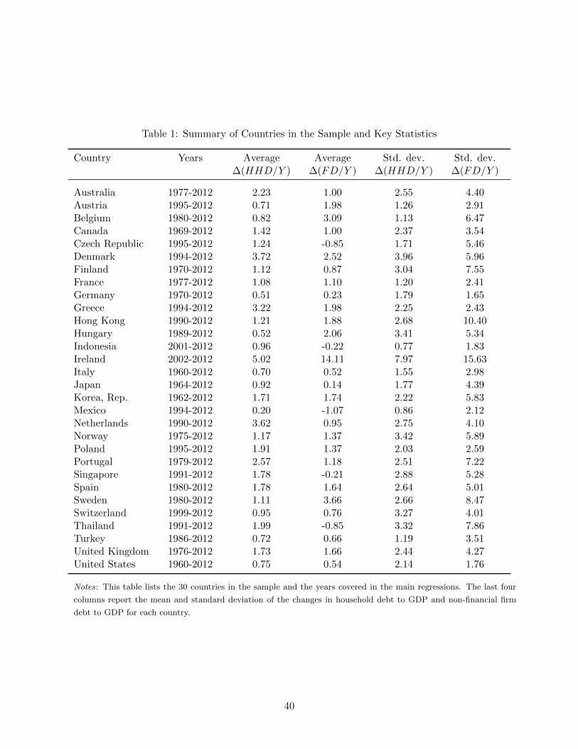
Table 1: Summary of Countries in the Sample and Key Statistics
Country Years Average∆(HHD/Y )
Average∆(FD/Y )
Std. dev.∆(HHD/Y )
Std. dev.∆(FD/Y )
Australia 1977-2012 2.23 1.00 2.55 4.40Austria 1995-2012 0.71 1.98 1.26 2.91Belgium 1980-2012 0.82 3.09 1.13 6.47Canada 1969-2012 1.42 1.00 2.37 3.54Czech Republic 1995-2012 1.24 -0.85 1.71 5.46Denmark 1994-2012 3.72 2.52 3.96 5.96Finland 1970-2012 1.12 0.87 3.04 7.55France 1977-2012 1.08 1.10 1.20 2.41Germany 1970-2012 0.51 0.23 1.79 1.65Greece 1994-2012 3.22 1.98 2.25 2.43Hong Kong 1990-2012 1.21 1.88 2.68 10.40Hungary 1989-2012 0.52 2.06 3.41 5.34Indonesia 2001-2012 0.96 -0.22 0.77 1.83Ireland 2002-2012 5.02 14.11 7.97 15.63Italy 1960-2012 0.70 0.52 1.55 2.98Japan 1964-2012 0.92 0.14 1.77 4.39Korea, Rep. 1962-2012 1.71 1.74 2.22 5.83Mexico 1994-2012 0.20 -1.07 0.86 2.12Netherlands 1990-2012 3.62 0.95 2.75 4.10Norway 1975-2012 1.17 1.37 3.42 5.89Poland 1995-2012 1.91 1.37 2.03 2.59Portugal 1979-2012 2.57 1.18 2.51 7.22Singapore 1991-2012 1.78 -0.21 2.88 5.28Spain 1980-2012 1.78 1.64 2.64 5.01Sweden 1980-2012 1.11 3.66 2.66 8.47Switzerland 1999-2012 0.95 0.76 3.27 4.01Thailand 1991-2012 1.99 -0.85 3.32 7.86Turkey 1986-2012 0.72 0.66 1.19 3.51United Kingdom 1976-2012 1.73 1.66 2.44 4.27United States 1960-2012 0.75 0.54 2.14 1.76
Notes: This table lists the 30 countries in the sample and the years covered in the main regressions. The last four
columns report the mean and standard deviation of the changes in household debt to GDP and non-financial firm
debt to GDP for each country.
40

Table 2: Summary Statistics
N Mean Median SD SDSD(∆y) Ser. Cor.
∆y 695 2.90 3.08 2.98 1.00 0.29∆3y 695 8.40 8.65 6.56 2.21 0.71∆(PD/Y ) 695 3.11 2.52 6.96 2.34 0.39∆3(PD/Y ) 695 8.52 7.28 16.04 5.39 0.74∆(HHD/Y ) 695 1.62 1.33 2.56 0.86 0.43∆3(HHD/Y ) 695 4.58 3.68 6.24 2.10 0.79∆(FD/Y ) 695 1.48 1.04 5.66 1.90 0.30∆3(FD/Y ) 695 3.89 3.11 12.21 4.10 0.69∆c 678 2.81 2.90 2.84 0.95 0.33∆cdur 469 4.91 5.35 9.27 3.12 0.21∆cnondur 469 1.53 1.47 2.53 0.85 0.26∆C/Y 690 -0.06 -0.01 1.17 0.39 0.04∆i 678 2.66 3.67 10.79 3.63 0.15∆g 688 2.84 2.60 2.79 0.94 0.26∆x 695 8.64 9.30 12.29 4.13 0.15∆m 695 8.08 9.55 13.87 4.66 0.12∆NX/Y 695 0.14 -0.01 2.11 0.71 0.03∆CA/Y 648 0.08 -0.02 2.29 0.77 -0.01∆sXC 695 -0.15 -0.07 1.80 0.61 0.04∆sMC 695 0.16 0.15 1.67 0.56 0.00∆reer 614 -0.03 0.59 6.75 2.27 0.05∆u 669 0.08 -0.01 1.08 0.36 0.34∆3u 662 0.19 -0.01 2.43 0.82 0.67∆3y
WEOt+3|t 484 9.41 8.60 3.76 1.26 0.50
∆3(yt+3 − yWEOt+3|t ) 484 -2.53 -1.79 5.35 1.80 0.54
∆3hpi 514 6.56 7.16 17.42 5.85 0.72∆3(GD/Y ) 627 1.73 1.16 9.92 3.33 0.71sprreal 622 0.43 0.40 2.11 0.71 0.42sprMS 517 1.15 0.99 1.52 0.51 0.45sprcorp 460 0.76 0.65 1.03 0.35 0.42
Notes: Log changes and ratios are multiplied by 100 to report changes in percentages or percent-
age points. ∆ and ∆3 denote to one-year and three-year changes, respectively. The variables
y, PD/Y,HHD/Y, FD/Y, c, cdur, cnondur, C/Y, i, g, x,m,NX/Y,CA/Y, sXC , sMC , reer, u, yWEOt+3|t , hpi,GD/Y, spr
real,
sprMS , and sprcorp denote log real GDP, private non-financial debt to GDP, household debt to GDP, non-financial
firm debt to GDP, log real consumption, log real durable consumption, log real nondurable consumption, consump-
tion to GDP, log real investment, log real government consumption, log nominal exports, log nominal imports,
net exports to GDP, current account to GDP, the share of consumption exports to total exports, the share of
consumption imports to total imports, log real effective exchange rate, the unemployment rate, the IMF Fall World
Economic Outlook time t forecast of growth from t to t+3, the log house price index, government debt to GDP, the
real 10 year government bond yield spread with respect to the United States, mortgage-sovereign spread, and the
corporate-sovereign spread, respectively.
41
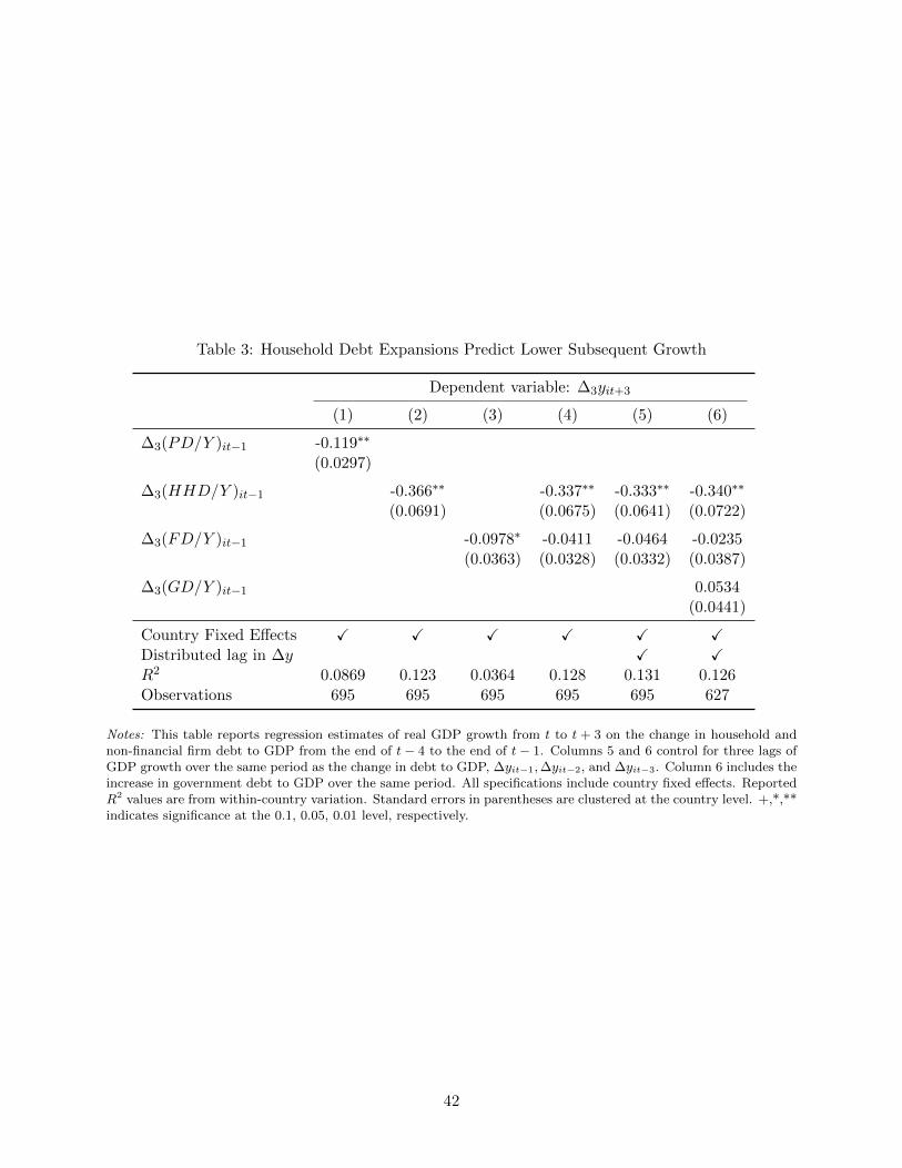
Table 3: Household Debt Expansions Predict Lower Subsequent Growth
Dependent variable: ∆3yit+3
(1) (2) (3) (4) (5) (6)
∆3(PD/Y )it−1 -0.119∗∗
(0.0297)
∆3(HHD/Y )it−1 -0.366∗∗ -0.337∗∗ -0.333∗∗ -0.340∗∗
(0.0691) (0.0675) (0.0641) (0.0722)
∆3(FD/Y )it−1 -0.0978∗ -0.0411 -0.0464 -0.0235(0.0363) (0.0328) (0.0332) (0.0387)
∆3(GD/Y )it−1 0.0534(0.0441)
Country Fixed Effects X X X X X XDistributed lag in ∆y X XR2 0.0869 0.123 0.0364 0.128 0.131 0.126Observations 695 695 695 695 695 627
Notes: This table reports regression estimates of real GDP growth from t to t + 3 on the change in household andnon-financial firm debt to GDP from the end of t− 4 to the end of t− 1. Columns 5 and 6 control for three lags ofGDP growth over the same period as the change in debt to GDP, ∆yit−1,∆yit−2, and ∆yit−3. Column 6 includes theincrease in government debt to GDP over the same period. All specifications include country fixed effects. ReportedR2 values are from within-country variation. Standard errors in parentheses are clustered at the country level. +,*,**indicates significance at the 0.1, 0.05, 0.01 level, respectively.
42
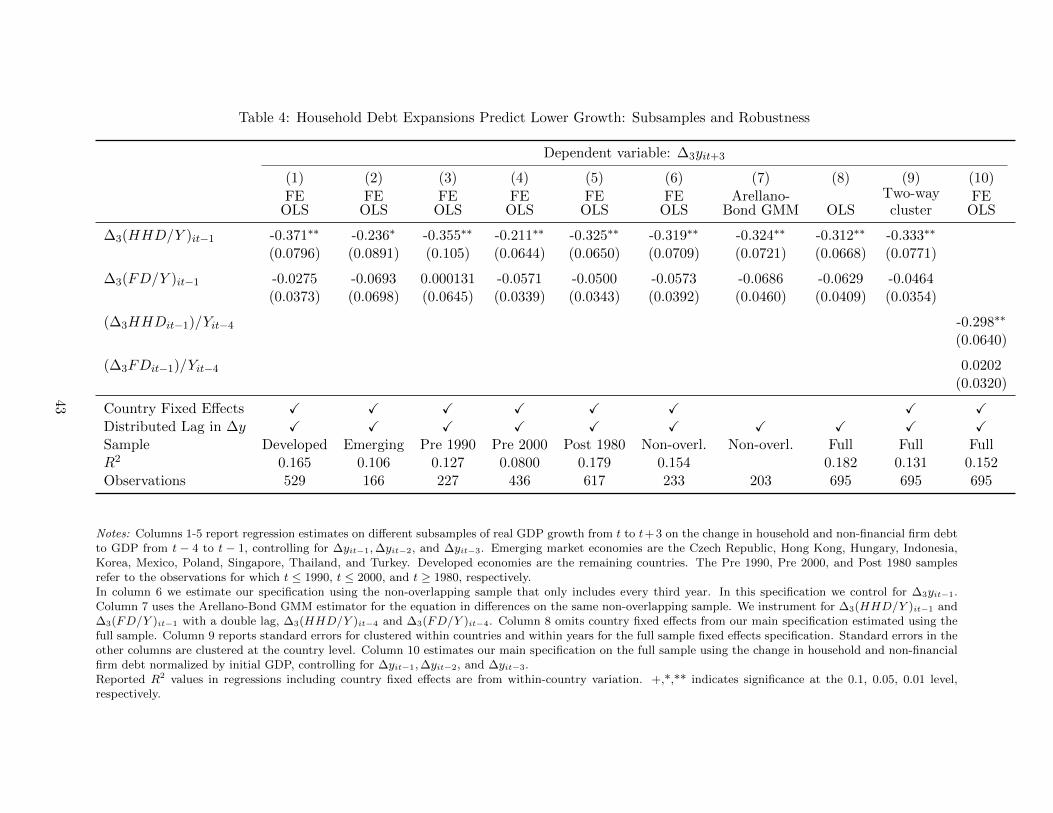
Table 4: Household Debt Expansions Predict Lower Growth: Subsamples and Robustness
Dependent variable: ∆3yit+3
(1) (2) (3) (4) (5) (6) (7) (8) (9) (10)
FEOLS
FEOLS
FEOLS
FEOLS
FEOLS
FEOLS
Arellano-Bond GMM OLS
Two-waycluster
FEOLS
∆3(HHD/Y )it−1 -0.371∗∗ -0.236∗ -0.355∗∗ -0.211∗∗ -0.325∗∗ -0.319∗∗ -0.324∗∗ -0.312∗∗ -0.333∗∗
(0.0796) (0.0891) (0.105) (0.0644) (0.0650) (0.0709) (0.0721) (0.0668) (0.0771)
∆3(FD/Y )it−1 -0.0275 -0.0693 0.000131 -0.0571 -0.0500 -0.0573 -0.0686 -0.0629 -0.0464(0.0373) (0.0698) (0.0645) (0.0339) (0.0343) (0.0392) (0.0460) (0.0409) (0.0354)
(∆3HHDit−1)/Yit−4 -0.298∗∗
(0.0640)
(∆3FDit−1)/Yit−4 0.0202(0.0320)
Country Fixed Effects X X X X X X X XDistributed Lag in ∆y X X X X X X X X X XSample Developed Emerging Pre 1990 Pre 2000 Post 1980 Non-overl. Non-overl. Full Full FullR2 0.165 0.106 0.127 0.0800 0.179 0.154 0.182 0.131 0.152Observations 529 166 227 436 617 233 203 695 695 695
Notes: Columns 1-5 report regression estimates on different subsamples of real GDP growth from t to t+3 on the change in household and non-financial firm debtto GDP from t − 4 to t − 1, controlling for ∆yit−1,∆yit−2, and ∆yit−3. Emerging market economies are the Czech Republic, Hong Kong, Hungary, Indonesia,Korea, Mexico, Poland, Singapore, Thailand, and Turkey. Developed economies are the remaining countries. The Pre 1990, Pre 2000, and Post 1980 samplesrefer to the observations for which t ≤ 1990, t ≤ 2000, and t ≥ 1980, respectively.In column 6 we estimate our specification using the non-overlapping sample that only includes every third year. In this specification we control for ∆3yit−1.Column 7 uses the Arellano-Bond GMM estimator for the equation in differences on the same non-overlapping sample. We instrument for ∆3(HHD/Y )it−1 and∆3(FD/Y )it−1 with a double lag, ∆3(HHD/Y )it−4 and ∆3(FD/Y )it−4. Column 8 omits country fixed effects from our main specification estimated using thefull sample. Column 9 reports standard errors for clustered within countries and within years for the full sample fixed effects specification. Standard errors in theother columns are clustered at the country level. Column 10 estimates our main specification on the full sample using the change in household and non-financialfirm debt normalized by initial GDP, controlling for ∆yit−1,∆yit−2, and ∆yit−3.Reported R2 values in regressions including country fixed effects are from within-country variation. +,*,** indicates significance at the 0.1, 0.05, 0.01 level,respectively.
43
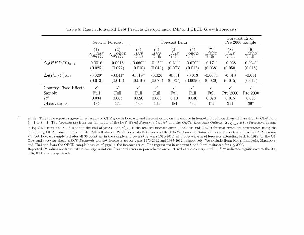
Table 5: Rise in Household Debt Predicts Overoptimistic IMF and OECD Growth Forecasts
Growth Forecast Forecast ErrorForecast Error
Pre 2000 Sample
(1) (2) (3) (4) (5) (6) (7) (8) (9)∆2y
IMFt+2|t ∆2y
OECDt+2|t eIMF
t+1|t eIMFt+2|t eIMF
t+3|t eOECDt+1|t eOECDt+2|t eIMFt+1|t eOECDt+1|t
∆3(HHD/Y )it−1 0.0016 0.0013 -0.060∗∗ -0.17∗∗ -0.31∗∗ -0.070∗∗ -0.17∗∗ -0.068 -0.064∗∗
(0.025) (0.022) (0.018) (0.043) (0.073) (0.013) (0.038) (0.050) (0.018)
∆3(FD/Y )it−1 -0.029∗ -0.041∗ -0.019+ -0.026 -0.031 -0.013 -0.0084 -0.013 -0.014(0.013) (0.015) (0.010) (0.025) (0.037) (0.0090) (0.020) (0.015) (0.012)
Country Fixed Effects X X X X X X X X XSample Full Full Full Full Full Full Full Pre 2000 Pre 2000R2 0.034 0.064 0.026 0.063 0.13 0.040 0.073 0.015 0.026Observations 484 471 590 484 484 594 471 331 367
Notes: This table reports regression estimates of GDP growth forecasts and forecast errors on the change in household and non-financial firm debt to GDP fromt − 4 to t − 1. The forecasts are from the fall issues of the IMF World Economic Outlook and the OECD Economic Outlook. ∆hy
ft+h|t is the forecasted change
in log GDP from t to t + h made in the Fall of year t, and eft+h|t is the realized forecast error. The IMF and OECD forecast errors are constructed using therealized log GDP change reported in the IMF’s Historical WEO Forecasts Database and the OECD Economic Outlook reports, respectively. The World EconomicOutlook forecast sample includes all 30 countries in the sample and covers the years 1990-2012, with one-year-ahead forecasts extending back to 1972 for the G7.One- and two-year-ahead OECD Economic Outlook forecasts are for years 1973-2012 and 1987-2012, respectively. We exclude Hong Kong, Indonesia, Singapore,and Thailand from the OECD sample because of gaps in the forecast series. The regressions in columns 8 and 9 are estimated for t ≤ 2000.Reported R2 values are from within-country variation. Standard errors in parentheses are clustered at the country level. +,*,** indicates significance at the 0.1,0.05, 0.01 level, respectively.
44
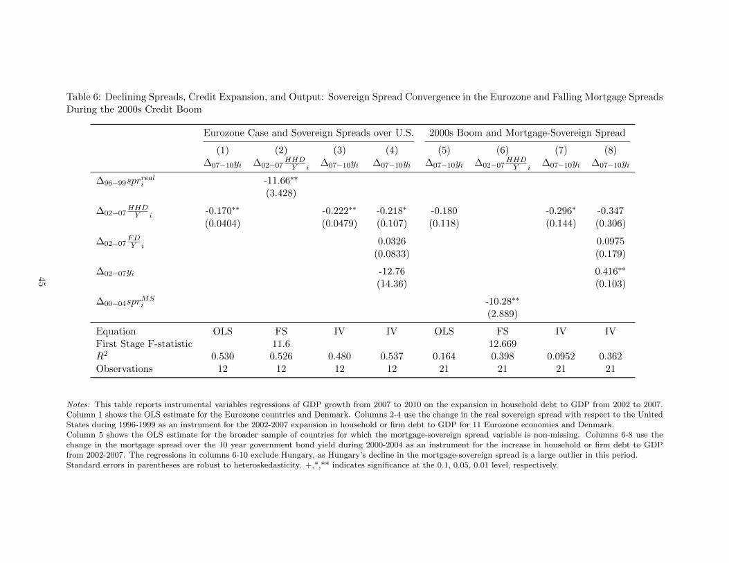
Table 6: Declining Spreads, Credit Expansion, and Output: Sovereign Spread Convergence in the Eurozone and Falling Mortgage SpreadsDuring the 2000s Credit Boom
Eurozone Case and Sovereign Spreads over U.S. 2000s Boom and Mortgage-Sovereign Spread
(1) (2) (3) (4) (5) (6) (7) (8)
∆07−10yi ∆02−07HHDY i
∆07−10yi ∆07−10yi ∆07−10yi ∆02−07HHDY i
∆07−10yi ∆07−10yi
∆96−99sprreali -11.66∗∗
(3.428)
∆02−07HHDY i
-0.170∗∗ -0.222∗∗ -0.218∗ -0.180 -0.296∗ -0.347
(0.0404) (0.0479) (0.107) (0.118) (0.144) (0.306)
∆02−07FDY i
0.0326 0.0975
(0.0833) (0.179)
∆02−07yi -12.76 0.416∗∗
(14.36) (0.103)
∆00−04sprMSi -10.28∗∗
(2.889)
Equation OLS FS IV IV OLS FS IV IVFirst Stage F-statistic 11.6 12.669R2 0.530 0.526 0.480 0.537 0.164 0.398 0.0952 0.362Observations 12 12 12 12 21 21 21 21
Notes: This table reports instrumental variables regressions of GDP growth from 2007 to 2010 on the expansion in household debt to GDP from 2002 to 2007.Column 1 shows the OLS estimate for the Eurozone countries and Denmark. Columns 2-4 use the change in the real sovereign spread with respect to the UnitedStates during 1996-1999 as an instrument for the 2002-2007 expansion in household or firm debt to GDP for 11 Eurozone economies and Denmark.Column 5 shows the OLS estimate for the broader sample of countries for which the mortgage-sovereign spread variable is non-missing. Columns 6-8 use thechange in the mortgage spread over the 10 year government bond yield during 2000-2004 as an instrument for the increase in household or firm debt to GDPfrom 2002-2007. The regressions in columns 6-10 exclude Hungary, as Hungary’s decline in the mortgage-sovereign spread is a large outlier in this period.Standard errors in parentheses are robust to heteroskedasticity. +,*,** indicates significance at the 0.1, 0.05, 0.01 level, respectively.
45
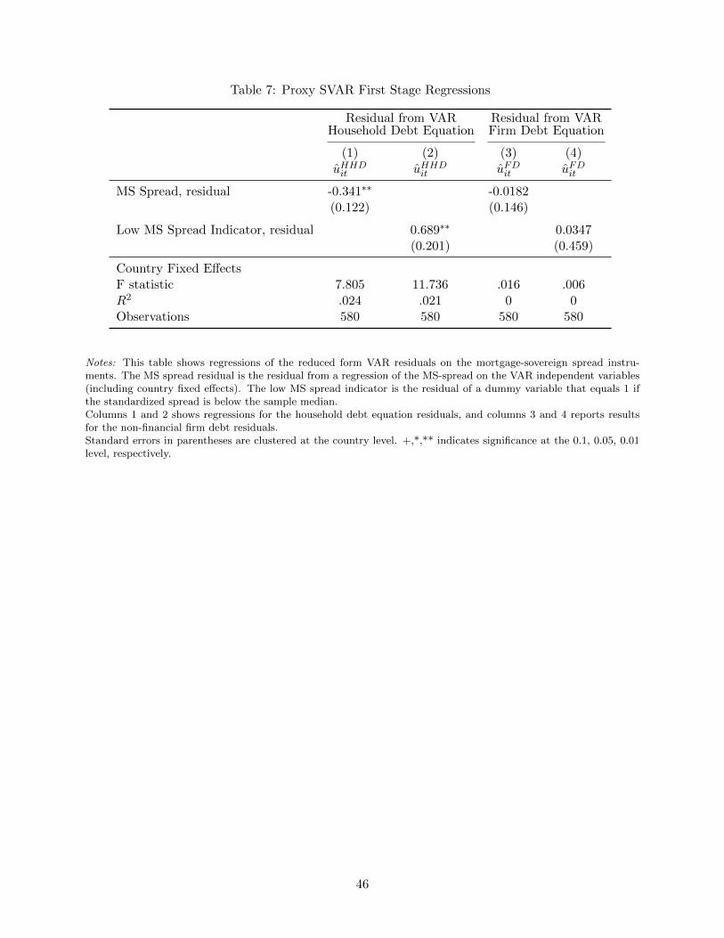
Table 7: Proxy SVAR First Stage Regressions
Residual from VARHousehold Debt Equation
Residual from VARFirm Debt Equation
(1) (2) (3) (4)uHHDit uHHDit uFDit uFDit
MS Spread, residual -0.341∗∗ -0.0182(0.122) (0.146)
Low MS Spread Indicator, residual 0.689∗∗ 0.0347(0.201) (0.459)
Country Fixed EffectsF statistic 7.805 11.736 .016 .006R2 .024 .021 0 0Observations 580 580 580 580
Notes: This table shows regressions of the reduced form VAR residuals on the mortgage-sovereign spread instru-ments. The MS spread residual is the residual from a regression of the MS-spread on the VAR independent variables(including country fixed effects). The low MS spread indicator is the residual of a dummy variable that equals 1 ifthe standardized spread is below the sample median.Columns 1 and 2 shows regressions for the household debt equation residuals, and columns 3 and 4 reports resultsfor the non-financial firm debt residuals.Standard errors in parentheses are clustered at the country level. +,*,** indicates significance at the 0.1, 0.05, 0.01level, respectively.
46
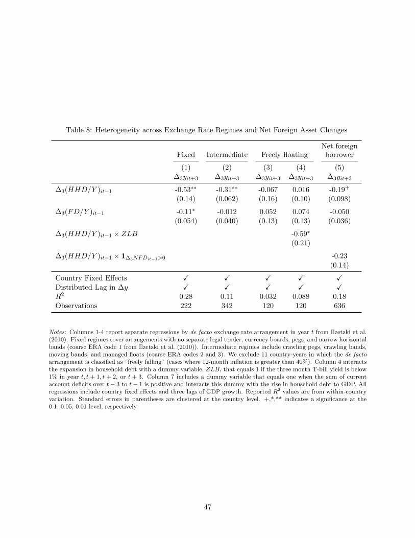
Table 8: Heterogeneity across Exchange Rate Regimes and Net Foreign Asset Changes
Fixed Intermediate Freely floatingNet foreignborrower
(1) (2) (3) (4) (5)∆3yit+3 ∆3yit+3 ∆3yit+3 ∆3yit+3 ∆3yit+3
∆3(HHD/Y )it−1 -0.53∗∗ -0.31∗∗ -0.067 0.016 -0.19+
(0.14) (0.062) (0.16) (0.10) (0.098)
∆3(FD/Y )it−1 -0.11∗ -0.012 0.052 0.074 -0.050(0.054) (0.040) (0.13) (0.13) (0.036)
∆3(HHD/Y )it−1 × ZLB -0.59∗
(0.21)
∆3(HHD/Y )it−1 × 1∆3NFDit−1>0 -0.23(0.14)
Country Fixed Effects X X X X XDistributed Lag in ∆y X X X X XR2 0.28 0.11 0.032 0.088 0.18Observations 222 342 120 120 636
Notes: Columns 1-4 report separate regressions by de facto exchange rate arrangement in year t from Ilzetzki et al.(2010). Fixed regimes cover arrangements with no separate legal tender, currency boards, pegs, and narrow horizontalbands (coarse ERA code 1 from Ilzetzki et al. (2010)). Intermediate regimes include crawling pegs, crawling bands,moving bands, and managed floats (coarse ERA codes 2 and 3). We exclude 11 country-years in which the de factoarrangement is classified as “freely falling” (cases where 12-month inflation is greater than 40%). Column 4 interactsthe expansion in household debt with a dummy variable, ZLB, that equals 1 if the three month T-bill yield is below1% in year t, t + 1, t + 2, or t + 3. Column 7 includes a dummy variable that equals one when the sum of currentaccount deficits over t− 3 to t− 1 is positive and interacts this dummy with the rise in household debt to GDP. Allregressions include country fixed effects and three lags of GDP growth. Reported R2 values are from within-countryvariation. Standard errors in parentheses are clustered at the country level. +,*,** indicates a significance at the0.1, 0.05, 0.01 level, respectively.
47
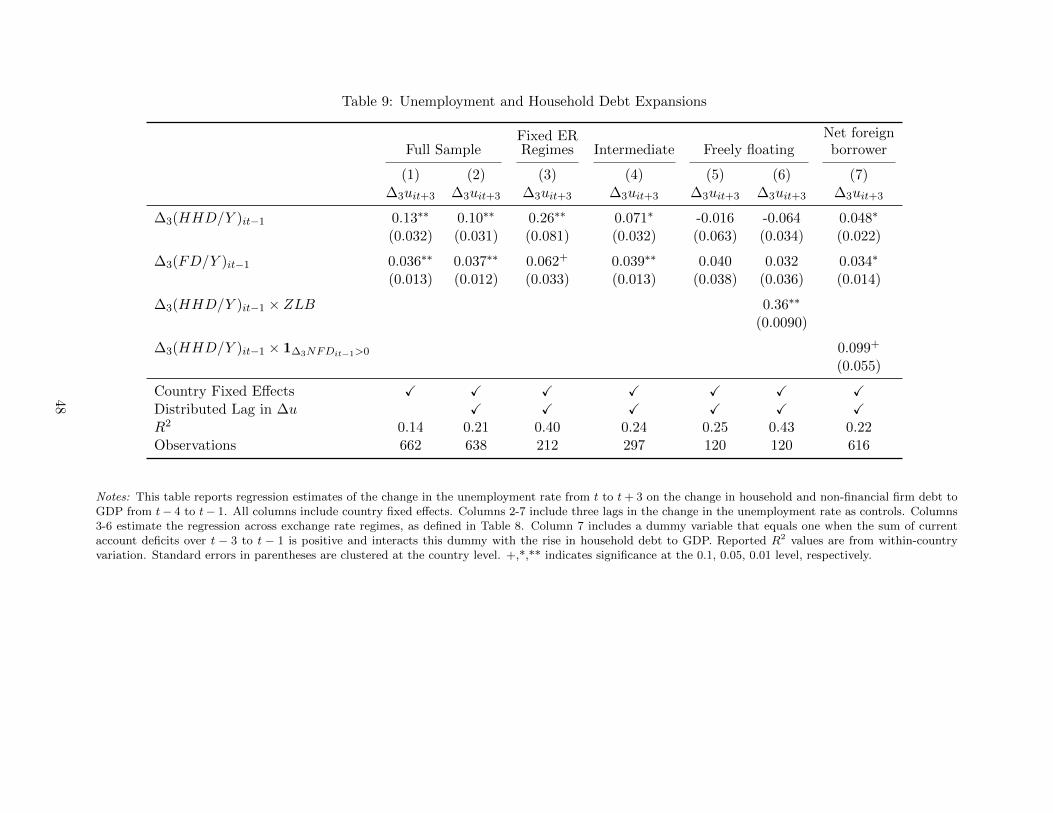
Table 9: Unemployment and Household Debt Expansions
Full SampleFixed ERRegimes Intermediate Freely floating
Net foreignborrower
(1) (2) (3) (4) (5) (6) (7)∆3uit+3 ∆3uit+3 ∆3uit+3 ∆3uit+3 ∆3uit+3 ∆3uit+3 ∆3uit+3
∆3(HHD/Y )it−1 0.13∗∗ 0.10∗∗ 0.26∗∗ 0.071∗ -0.016 -0.064 0.048∗
(0.032) (0.031) (0.081) (0.032) (0.063) (0.034) (0.022)
∆3(FD/Y )it−1 0.036∗∗ 0.037∗∗ 0.062+ 0.039∗∗ 0.040 0.032 0.034∗
(0.013) (0.012) (0.033) (0.013) (0.038) (0.036) (0.014)
∆3(HHD/Y )it−1 × ZLB 0.36∗∗
(0.0090)
∆3(HHD/Y )it−1 × 1∆3NFDit−1>0 0.099+
(0.055)
Country Fixed Effects X X X X X X XDistributed Lag in ∆u X X X X X XR2 0.14 0.21 0.40 0.24 0.25 0.43 0.22Observations 662 638 212 297 120 120 616
Notes: This table reports regression estimates of the change in the unemployment rate from t to t+ 3 on the change in household and non-financial firm debt toGDP from t− 4 to t− 1. All columns include country fixed effects. Columns 2-7 include three lags in the change in the unemployment rate as controls. Columns3-6 estimate the regression across exchange rate regimes, as defined in Table 8. Column 7 includes a dummy variable that equals one when the sum of currentaccount deficits over t − 3 to t − 1 is positive and interacts this dummy with the rise in household debt to GDP. Reported R2 values are from within-countryvariation. Standard errors in parentheses are clustered at the country level. +,*,** indicates significance at the 0.1, 0.05, 0.01 level, respectively.
48

Table 10: Household Debt Increases Finance Consumption Booms
(1) (2) (3) (4) (5) (6) (7) (8) (9)
∆1CY it
∆1IY it
∆1NXY it
∆1CAY it
∆1sMCit ∆1s
XCit ∆1
Cnondur
Y it∆1
Cdur
Y it∆1
Cservices
Y it
∆1(HHD/Y )it 0.120∗∗ 0.0174 -0.173∗ -0.185∗ 0.152∗∗ 0.0371 0.0432∗∗ 0.0333∗∗ 0.0709∗∗
(0.0402) (0.0545) (0.0665) (0.0843) (0.0361) (0.0326) (0.0127) (0.00664) (0.0185)
∆1(FD/Y )it 0.0249+ -0.0194 -0.0167 -0.0125 -0.0261 -0.0400+ 0.0200∗∗ -0.0161∗∗ 0.0293∗∗
(0.0126) (0.0271) (0.0205) (0.0186) (0.0167) (0.0204) (0.00544) (0.00335) (0.00826)
Country Fixed Effects X X X X X X X X XR2 0.0825 0.00216 0.0408 0.0374 0.0417 0.0129 0.0802 0.0647 0.138Observations 690 688 695 648 695 695 466 466 466
Notes: This table shows the contemporaneous correlation between the change in household and firm debt to GDP and the change in consumption to GDP,investment to GDP, net exports to GDP, current account to GDP, the share of consumption imports in total imports, the share of consumption exports in totalexports, non-durable consumption to GDP, durable consumption to GDP, and services consumption to GDP. All specifications include country fixed effects.Reported R2 values are from within-country variation. Standard errors in parentheses are clustered at the country level. +,*,** indicates significance at the 0.1,0.05, 0.01 level, respectively.
49
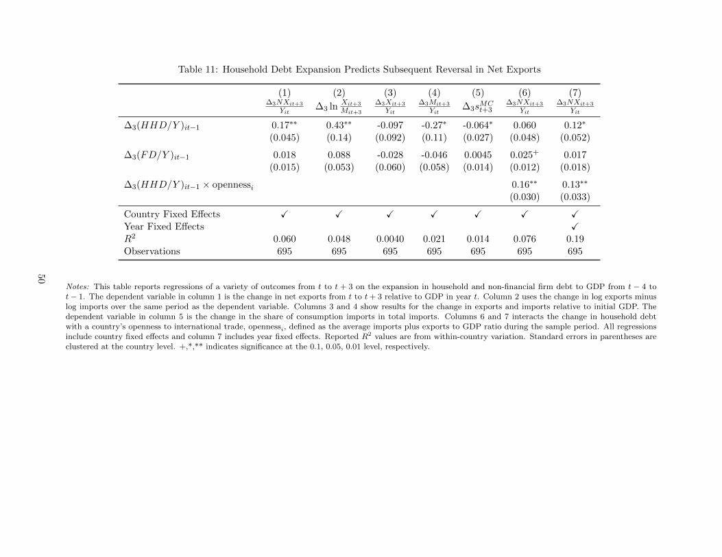
Table 11: Household Debt Expansion Predicts Subsequent Reversal in Net Exports
(1) (2) (3) (4) (5) (6) (7)∆3NXit+3
Yit∆3 ln Xit+3
Mit+3
∆3Xit+3
Yit
∆3Mit+3
Yit∆3s
MCt+3
∆3NXit+3
Yit
∆3NXit+3
Yit
∆3(HHD/Y )it−1 0.17∗∗ 0.43∗∗ -0.097 -0.27∗ -0.064∗ 0.060 0.12∗
(0.045) (0.14) (0.092) (0.11) (0.027) (0.048) (0.052)
∆3(FD/Y )it−1 0.018 0.088 -0.028 -0.046 0.0045 0.025+ 0.017(0.015) (0.053) (0.060) (0.058) (0.014) (0.012) (0.018)
∆3(HHD/Y )it−1 × opennessi 0.16∗∗ 0.13∗∗
(0.030) (0.033)
Country Fixed Effects X X X X X X XYear Fixed Effects XR2 0.060 0.048 0.0040 0.021 0.014 0.076 0.19Observations 695 695 695 695 695 695 695
Notes: This table reports regressions of a variety of outcomes from t to t + 3 on the expansion in household and non-financial firm debt to GDP from t − 4 tot− 1. The dependent variable in column 1 is the change in net exports from t to t+ 3 relative to GDP in year t. Column 2 uses the change in log exports minuslog imports over the same period as the dependent variable. Columns 3 and 4 show results for the change in exports and imports relative to initial GDP. Thedependent variable in column 5 is the change in the share of consumption imports in total imports. Columns 6 and 7 interacts the change in household debtwith a country’s openness to international trade, opennessi, defined as the average imports plus exports to GDP ratio during the sample period. All regressionsinclude country fixed effects and column 7 includes year fixed effects. Reported R2 values are from within-country variation. Standard errors in parentheses areclustered at the country level. +,*,** indicates significance at the 0.1, 0.05, 0.01 level, respectively.
50

Table 12: Global Household and Firm Debt and Global Growth
Dependent variable: global average ∆3yt+3
(1) (2) (3) (4) (5)
Global ∆3HHDY t−1
-1.094∗∗ -1.097∗∗ -0.966∗∗ -1.095∗∗
(0.300) (0.311) (0.252) (0.266)
Global ∆3FDY t−1
-0.103 0.00896 -0.0756 0.0747
(0.192) (0.177) (0.149) (0.199)
Global ∆yt−1 0.341 0.391(0.244) (0.276)
Global ∆yt−2 0.390+ 0.534∗∗
(0.224) (0.178)
Global ∆yt−3 0.477+ 0.445(0.258) (0.315)
Sample Full Full Full Full Pre 2000R2 .295 .007 .295 .471 .455Observations 46 46 46 46 37
Notes: This table reports time series regressions of the sample average real GDP growth from t to t+3 on the sampleaverage change in household and firm debt to GDP from t− 4 to t− 1. Newey-West standard errors in parenthesesare computed with 6 lags. +,*,** indicates significance at the 0.1, 0.05, 0.01 level, respectively.
51
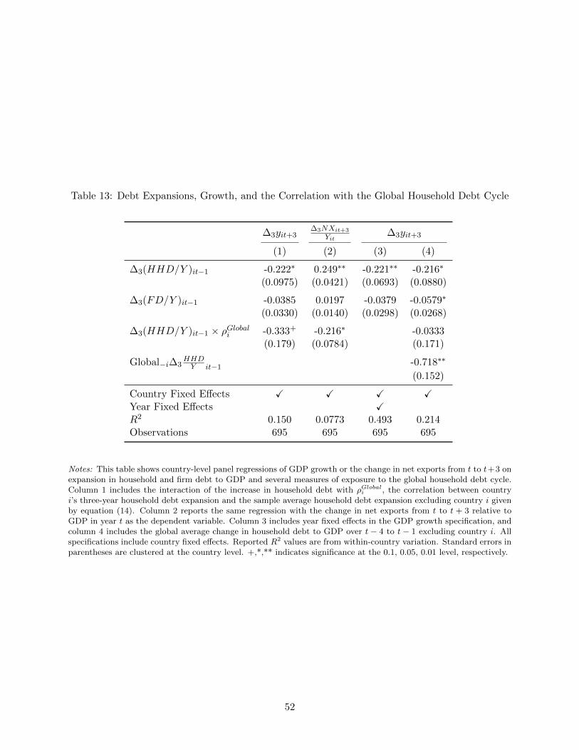
Table 13: Debt Expansions, Growth, and the Correlation with the Global Household Debt Cycle
∆3yit+3∆3NXit+3
Yit∆3yit+3
(1) (2) (3) (4)
∆3(HHD/Y )it−1 -0.222∗ 0.249∗∗ -0.221∗∗ -0.216∗
(0.0975) (0.0421) (0.0693) (0.0880)
∆3(FD/Y )it−1 -0.0385 0.0197 -0.0379 -0.0579∗
(0.0330) (0.0140) (0.0298) (0.0268)
∆3(HHD/Y )it−1 × ρGlobali -0.333+ -0.216∗ -0.0333(0.179) (0.0784) (0.171)
Global−i∆3HHDY it−1
-0.718∗∗
(0.152)
Country Fixed Effects X X X XYear Fixed Effects XR2 0.150 0.0773 0.493 0.214Observations 695 695 695 695
Notes: This table shows country-level panel regressions of GDP growth or the change in net exports from t to t+3 onexpansion in household and firm debt to GDP and several measures of exposure to the global household debt cycle.Column 1 includes the interaction of the increase in household debt with ρGlobali , the correlation between countryi’s three-year household debt expansion and the sample average household debt expansion excluding country i givenby equation (14). Column 2 reports the same regression with the change in net exports from t to t + 3 relative toGDP in year t as the dependent variable. Column 3 includes year fixed effects in the GDP growth specification, andcolumn 4 includes the global average change in household debt to GDP over t − 4 to t − 1 excluding country i. Allspecifications include country fixed effects. Reported R2 values are from within-country variation. Standard errors inparentheses are clustered at the country level. +,*,** indicates significance at the 0.1, 0.05, 0.01 level, respectively.
52
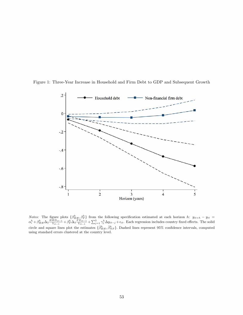
Figure 1: Three-Year Increase in Household and Firm Debt to GDP and Subsequent Growth
Notes: The figure plots {βhHH , βhF } from the following specification estimated at each horizon h: yit+h − yit =
αhi +βhHH∆3HHDit−1
Yit−1+βhF∆3
FDit−1
Yit−1+∑3j=1 γ
hj ∆yit−j + εit. Each regression includes country fixed effects. The solid
circle and square lines plot the estimates {βhHH , βhNF }. Dashed lines represent 95% confidence intervals, computedusing standard errors clustered at the country level.
53

Figure 2: Household Debt to GDP Expansion and Growth
(a) Household Debt
(b) Household Debt, Partial Correlation (c) NF Firm Debt, Partial Correlation
Notes: This figure plots the relationship between GDP growth from t to t + 3 and the expansion in household andfirm debt to GDP from t − 4 to t − 1. Each point refers to year t. The dashed line is the non-parametric plot ofGDP growth from t to t+ 3 against the increase in household or firm debt to GDP from t− 4 to t− 1. In panels (b)household debt is partialed out with the expansion in non-financial firm debt to GDP, while in panel (c) non-financialfirm debt is partialed out with the expansion in household debt to GDP.
54
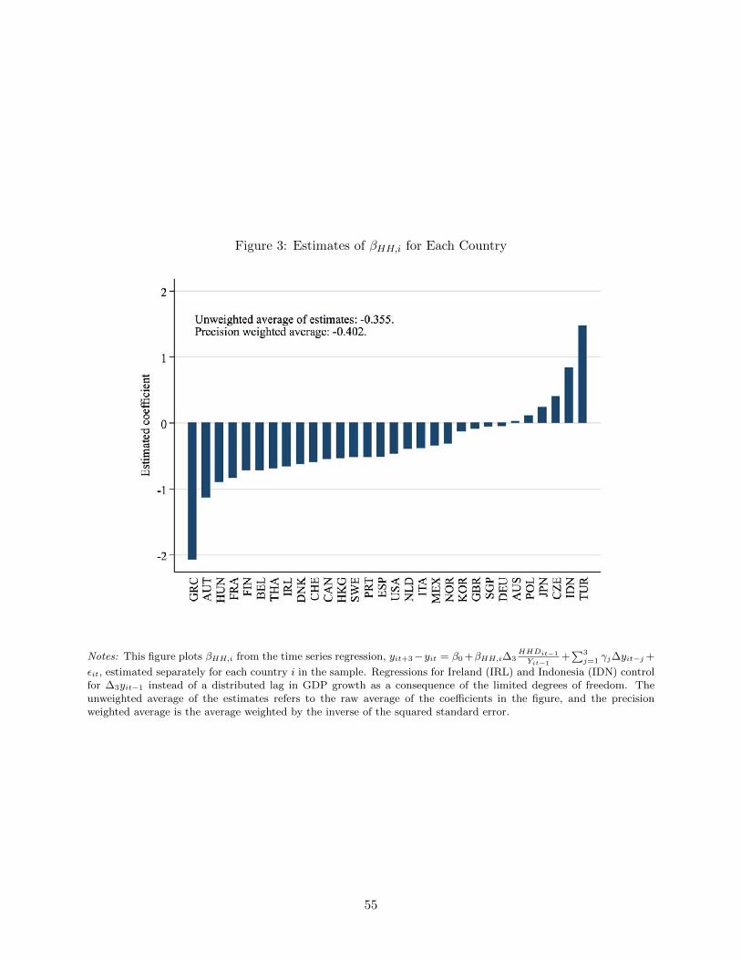
Figure 3: Estimates of βHH,i for Each Country
Notes: This figure plots βHH,i from the time series regression, yit+3−yit = β0 +βHH,i∆3HHDit−1
Yit−1+∑3j=1 γj∆yit−j+
εit, estimated separately for each country i in the sample. Regressions for Ireland (IRL) and Indonesia (IDN) controlfor ∆3yit−1 instead of a distributed lag in GDP growth as a consequence of the limited degrees of freedom. Theunweighted average of the estimates refers to the raw average of the coefficients in the figure, and the precisionweighted average is the average weighted by the inverse of the squared standard error.
55
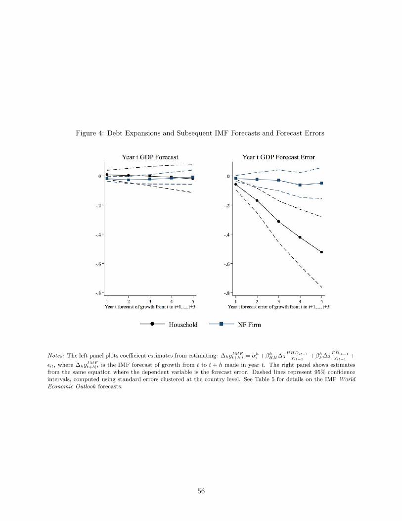
Figure 4: Debt Expansions and Subsequent IMF Forecasts and Forecast Errors
Notes: The left panel plots coefficient estimates from estimating: ∆hyIMFt+h|t = αhi +βhHH∆3
HHDit−1
Yit−1+βhF∆3
FDit−1
Yit−1+
εit, where ∆hyIMFt+h|t is the IMF forecast of growth from t to t + h made in year t. The right panel shows estimates
from the same equation where the dependent variable is the forecast error. Dashed lines represent 95% confidenceintervals, computed using standard errors clustered at the country level. See Table 5 for details on the IMF WorldEconomic Outlook forecasts.
56
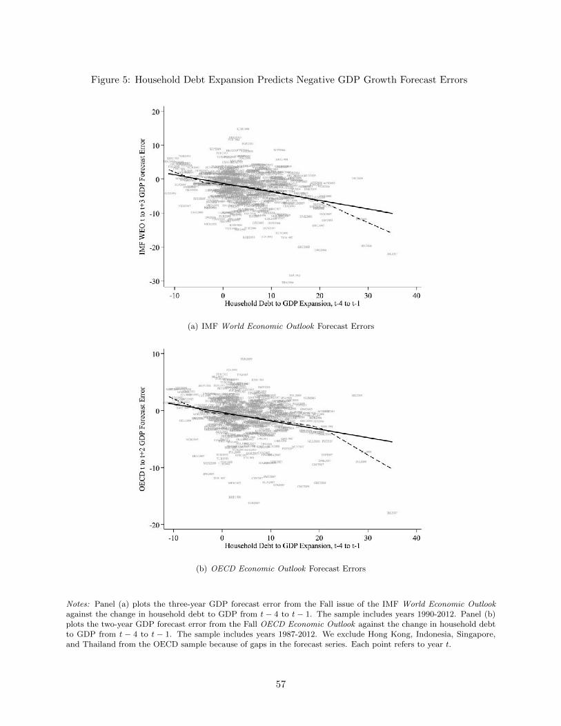
Figure 5: Household Debt Expansion Predicts Negative GDP Growth Forecast Errors
(a) IMF World Economic Outlook Forecast Errors
(b) OECD Economic Outlook Forecast Errors
Notes: Panel (a) plots the three-year GDP forecast error from the Fall issue of the IMF World Economic Outlookagainst the change in household debt to GDP from t − 4 to t − 1. The sample includes years 1990-2012. Panel (b)plots the two-year GDP forecast error from the Fall OECD Economic Outlook against the change in household debtto GDP from t − 4 to t − 1. The sample includes years 1987-2012. We exclude Hong Kong, Indonesia, Singapore,and Thailand from the OECD sample because of gaps in the forecast series. Each point refers to year t.
57
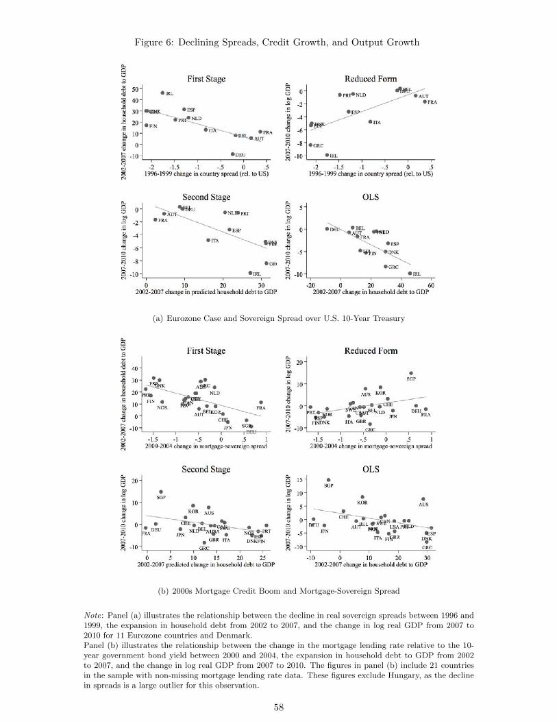
Figure 6: Declining Spreads, Credit Growth, and Output Growth
(a) Eurozone Case and Sovereign Spread over U.S. 10-Year Treasury
(b) 2000s Mortgage Credit Boom and Mortgage-Sovereign Spread
Note: Panel (a) illustrates the relationship between the decline in real sovereign spreads between 1996 and1999, the expansion in household debt from 2002 to 2007, and the change in log real GDP from 2007 to2010 for 11 Eurozone countries and Denmark.Panel (b) illustrates the relationship between the change in the mortgage lending rate relative to the 10-year government bond yield between 2000 and 2004, the expansion in household debt to GDP from 2002to 2007, and the change in log real GDP from 2007 to 2010. The figures in panel (b) include 21 countriesin the sample with non-missing mortgage lending rate data. These figures exclude Hungary, as the declinein spreads is a large outlier for this observation.
58
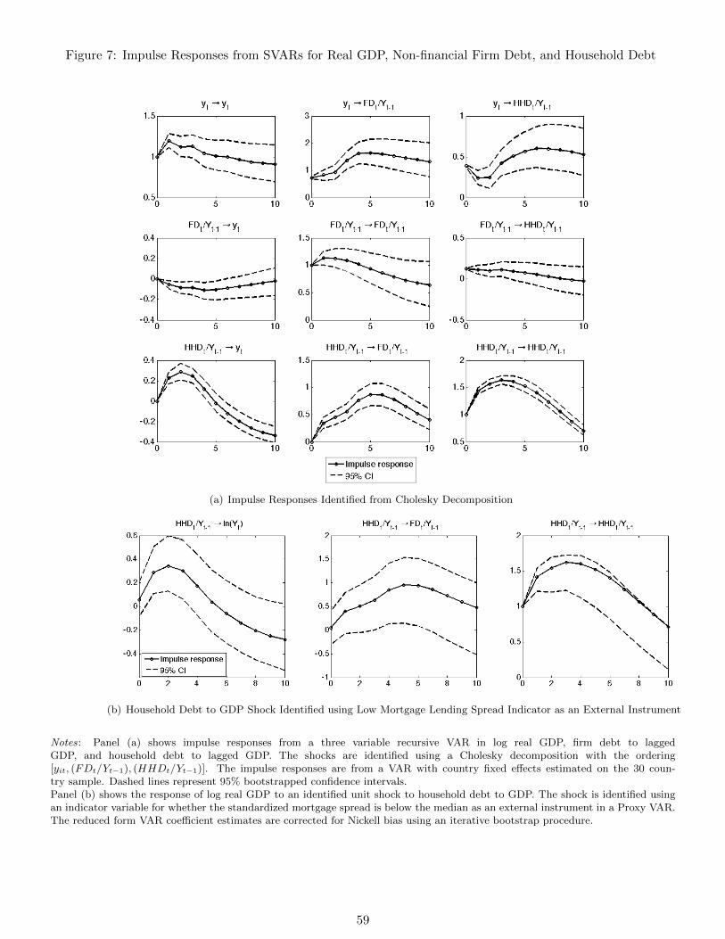
Figure 7: Impulse Responses from SVARs for Real GDP, Non-financial Firm Debt, and Household Debt
(a) Impulse Responses Identified from Cholesky Decomposition
(b) Household Debt to GDP Shock Identified using Low Mortgage Lending Spread Indicator as an External Instrument
Notes: Panel (a) shows impulse responses from a three variable recursive VAR in log real GDP, firm debt to laggedGDP, and household debt to lagged GDP. The shocks are identified using a Cholesky decomposition with the ordering[yit, (FDt/Yt−1), (HHDt/Yt−1)]. The impulse responses are from a VAR with country fixed effects estimated on the 30 coun-try sample. Dashed lines represent 95% bootstrapped confidence intervals.Panel (b) shows the response of log real GDP to an identified unit shock to household debt to GDP. The shock is identified usingan indicator variable for whether the standardized mortgage spread is below the median as an external instrument in a Proxy VAR.The reduced form VAR coefficient estimates are corrected for Nickell bias using an iterative bootstrap procedure.
59
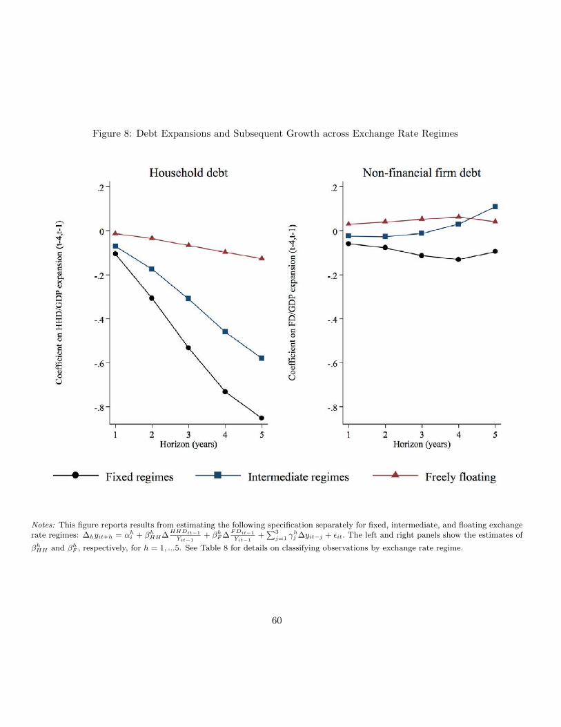
Figure 8: Debt Expansions and Subsequent Growth across Exchange Rate Regimes
Notes: This figure reports results from estimating the following specification separately for fixed, intermediate, and floating exchangerate regimes: ∆hyit+h = αhi + βhHH∆
HHDit−1
Yit−1+ βhF∆
FDit−1
Yit−1+∑3j=1 γ
hj ∆yit−j + εit. The left and right panels show the estimates of
βhHH and βhF , respectively, for h = 1, ...5. See Table 8 for details on classifying observations by exchange rate regime.
60
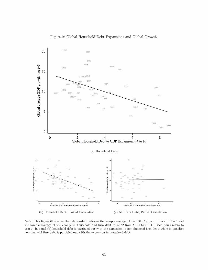
Figure 9: Global Household Debt Expansions and Global Growth
(a) Household Debt
(b) Household Debt, Partial Correlation (c) NF Firm Debt, Partial Correlation
Note: This figure illustrates the relationship between the sample average of real GDP growth from t to t + 3 andthe sample average of the change in household and firm debt to GDP from t − 4 to t − 1. Each point refers toyear t. In panel (b) household debt is partialed out with the expansion in non-financial firm debt, while in panel(c)non-financial firm debt is partialed out with the expansion in household debt.
61

Figure 10: Correlation with World Household Debt Cycle
Note: This figure shows the correlation between the three-year household debt to change for country i and the average
change for all countries excluding i: corr((
∆3HHDY
)it, 1N−1
∑j 6=i(∆3
HHDY
)jt
).
62