Household and Plot Level Impact of Sustainable Land

and Watershed Management (SLWM) Practices in the

Blue Nile

Emily Schmidt and Fanaye Tadesse

Development Strategy and Governance Division, International Food Policy Research

Institute – Ethiopia Strategy Support Program II, Ethiopia

IFPRI-ADDIS ABABA P.O. Box 5689 Addis Ababa, Ethiopia Tel: +251-11-646-2921 Fax: +251-11-646-2318 E-mail: ifpri-addis@cgiar.org http://essp.ifpri.info/

IFPRI HEADQUARTERS

International Food Policy Research Institute 2033 K Street, NW • Washington, DC 20006-1002 USA Tel: +1-202-862-5600 Skype: IFPRIhomeoffice Fax: +1-202-467-4439 E-mail: ifpri@cgiar.org http://www.ifpri.org

ESSP II Working Paper 42

Ethiopia Strategy Support Program II (ESSP II)

ESSP II Working Paper 42

August 2012

ii

THE ETHIOPIA STRATEGY SUPPORT PROGRAM II (ESSP II)

WORKING PAPERS

ABOUT ESSP II

The Ethiopia Strategy Support Program II is an initiative to strengthen evidence-based policymaking in Ethiopia in the areas of rural and agricultural development. Facilitated by the International Food Policy Research Institute (IFPRI), ESSP II works closely with the government of Ethiopia, the Ethiopian Development Research Institute (EDRI), and other development partners to provide information relevant for the design and implementation of Ethiopia’s agricultural and rural development strategies. For more information, see http://www.ifpri.org/book-757/ourwork/program/ethiopia-strategy-support-program or http://essp.ifpri.info/ or http://www.edri.org.et/.

ABOUT THESE WORKING PAPERS

The Ethiopia Strategy Support Program II (ESSP II) Working Papers contain preliminary material and research results from IFPRI and/or its partners in Ethiopia. The papers are not subject to a formal peer review. They are circulated in order to stimulate discussion and critical comment. The opinions are those of the authors and do not necessarily reflect those of their home institutions or supporting organizations.

About the Author(s)

Emily Schmidt: Country Program Coordinator / GIS specialist, Development Strategy and Governance Division, International Food Policy Research Institute (IFPRI)

Fanaye Tadesse: Research Officer, Ethiopia Strategy Support Program II, International Food Policy Research Institute (IFPRI)

iii

Household and Plot Level Impact of Sustainable Land

and Watershed Management (SLWM) Practices in the

Blue Nile

Emily Schmidt and Fanaye Tadesse

Development Strategy and Governance Division, International Food Policy Research

Institute – Ethiopia Strategy Support Program II, Ethiopia

Copyright © 2012 International Food Policy Research Institute. All rights reserved. Sections of this material may be reproduced for personal and not-for-profit use without the express written permission of but with acknowledgment to IFPRI. To reproduce the material contained herein for profit or commercial use requires express written permission. To obtain permission, contact the Communications Division at ifpri-copyright@cgiar.org.

iv

Table of Contents

Abstract ................................................................................................................................ vi

1. Introduction ...................................................................................................................... 1

2. Background ..................................................................................................................... 2

3. Survey data ..................................................................................................................... 4

4. Household characteristics and perception of SLWM structures ........................................ 6

5. Methodology .................................................................................................................. 10

5.1. Nearest neighbor matching ...................................................................................... 10

5.2. Dose response and treatment effect estimates ........................................................ 11

6. Results .......................................................................................................................... 13

6.1. Nearest neighbor matching ...................................................................................... 13

6.1.1. Determinants of adoption ................................................................................... 14

6.1.2. Impacts of adoption ............................................................................................ 15

6.2. Dose response and continuous treatment effect estimation results .......................... 17

6.2.1. Payoff period ...................................................................................................... 17

6.2.2. Cost benefit ........................................................................................................ 20

7. Conclusion ..................................................................................................................... 22

Appendix ............................................................................................................................. 23

References .......................................................................................................................... 26

v

List of Tables

Table 3.1—Survey sample selection (number of households surveyed) by program and stratification ....................................................................................................... 4

Table 4.1—Households using SLWM on private land ........................................................... 7

Table 4.2—Production patterns by woreda ........................................................................... 8

Table 4.3—Household characteristics of adopter and non-adopter households .................... 9

Table 6.1—Average household-level impact of SLWM adoption (single difference estimates) ........................................................................................................ 16

Table 6.2—Average plot-level impact of SLWM adoption (single difference estimates) ...... 16

Table 6.3—Average number of years the information providers report to benefit from SLWM adoption ............................................................................................... 17

Table 6.4—Test for equality of means between treatment groups ...................................... 18

Table 6.5—Marginal effect per extra year of maintenance .................................................. 19

Table 6.6—Cost-benefit of investing in SLWM infrastructure (1992–2009) ......................... 21

List of Figures

Figure 3.1—Spatial distribution of survey sites ...................................................................... 5

Figure 4.1—SLWM activities implemented in the village (percent of total households) .......... 6

Figure 6.1—Percent of total plots under SLWM on private land (1937–2009) ...................... 14

Appendix

Appendix Table A.1—Household probit results: Determinants of SLWM adoption 1992–2009 (1985–2002 E.C.) .................................................................... 23

Appendix Table A.2—Plot-level probit results: Determinants of SLWM adoption 1992–2009 (1985–2002 E.C.) ..................................................................... 24

Appendix Table A.3—First stage Maximum likelihood estimates on treatment level ............ 24

Appendix Table A.4—Second stage OLS Estimates on log of value of production .............. 24

Appendix A.5—Dose response function and Treatment effect function ................................ 25

vi

Abstract

Land degradation and water shortages are major issues in developing countries, contributing to reduced economic output, lower growth potential and increased poverty. The immediate trade-off between short-term welfare and long-term agricultural development in the highland regions of Ethiopia represents a challenge to successful economic development in a predominantly agricultural-based economy. Although previous studies investigated country-level economic costs of sustainable land and watershed management (SLWM) in Ethiopia, few quantitative assessments of household level SLWM adoption and maintenance, linked to benefit payoff horizons and magnitude, exist in recent literature.

We employ nearest-neighbor matching techniques to measure the impact of adopting specific SLWM technologies on value of production. Results suggest that households that adopted terraces, bunds, or check dams within the first period of the study period (1992–2002) experience a 15.2 percent higher value of production in 2010, while late adopters (farmers that adopted SLWM between 2003–2009) have no significant increases in value of production.

We repeat this analysis at plot level using continuous treatment effects analysis in order to take into account differences in treatment (defined as years a plot has been under SLWM investment). Results suggest that maintenance of SLWM structures is crucial to reap significant benefits from investment. Plots with SLWM infrastructure that are maintained for at least 7 years have a positive increase in value of production at the end of the 7th year, while those that received investments more recently or lacked continuous maintenance do not experience a statistically significant increase in value of production. In addition, we find that the marginal benefit of sustaining SLWM increases over time at an increasing rate.

Finally, we briefly discuss the benefits and costs of implementing SLWM for individual farmers and calculate an approximate net present value of investing in such infrastructure. We find that although value of production increases given these investments, the benefit may not always outweigh the costs of implementation, and policy measures to incentivize construction and maintenance may be needed.

Keywords: Ethiopia, sustainable land management, soil and water conservation, impact evaluation, propensity score matching

1

1. Introduction

Land degradation and water shortages are major development challenges in developing countries, contributing to reduced economic output, lower growth potential, and increased poverty. The immediate trade-off between short-term welfare (off-farm wage labor opportunities) and long-term agricultural development (investment in on-farm sustainable land management activities) in the highland regions of Ethiopia represents a large challenge to economic development in a predominantly agricultural based economy. Not only does prevailing agricultural land use and high rural population pressure intensify land and watershed degradation within the area, but the seasonally heavy rainfall, mountainous terrain, and advanced deforestation risks decreasing agricultural productivity to unsustainable levels.

Over the last two decades, the Ethiopian government and a variety of development partners have invested in a myriad of sustainable land and watershed management (SLWM) programs with an emphasis on local community and household participation in constructing and maintaining key infrastructures on public and private land. Thus far, studies suggest that long-term maintenance of such structures is not common among rural communities (Shiferaw and Holden 1998; Tadesse and Belay 2004; WFP 2005). This paper adds to these studies by identifying household and plot level determinants of SLWM program adoption and calculating impact of adoption utilizing a 2010 baseline survey. The survey collected data on participation in current and past SLWM activities at the individual, household, and community level within the Blue Nile basin in Ethiopia.

We use a nearest-neighbor matching technique developed by Abadie and Imbens (2002) to measure the impact of adopting specific SLWM technologies on value of production and livestock holdings. In addition we employ a continuous treatment effect estimation method to understand the length of time a plot of land must be maintained under SLWM infrastructure in order to experience a benefit, and then calculate marginal benefits of each additional year of maintenance. Results suggest that threshold effects are present whereby farmers must maintain SLWM structures for at least 7 years before experiencing any significant benefits. Although benefits are not realized immediately, analysis of marginal effects of adopting and maintaining terraces, bunds, or check dams suggests that the marginal return to maintenance increases at an increasing rate from 7 to 15 years after construction of the structures.

The remainder of the paper is organized as follows. Section 2 provides a background to Ethiopia’s current policy objectives for SLWM, as well as a review of current literature on impact analysis of soil and water conservation structures in Ethiopia and abroad. Section 3 describes the survey design and sampling strategy. Section 4 provides an overview of household characteristics by district (woreda), perceptions of past and ongoing SLWM programs and investments, and descriptive statistics for treatment (adopters of SLWM) and control groups at the household level. Section 5 discusses the methods used in this paper. Section 6 provides results from nearest neighbor matching estimates of program impact on household and plot-level value of production and livestock holdings. We also present results from continuous treatment effect estimates whereby level of treatment is defined as the number of years households have been implementing specific SLM activities on individual plots. In addition, we contextualize these marginal benefits within a benefit-cost framework. Finally, we summarize and conclude in section 7.

2

2. Background

Under Ethiopia’s previous five-year economic development plan, the Plan for Accelerated and Sustained Development to End Poverty (PASDEP), 2005/06–2009/10, the government invested in a series of land and watershed management activities with the goal of augmenting agricultural production. These activities included piloting and implementing locally appropriate, community-based approaches to watershed management; scaling up successful models for watershed conservation; and strengthening natural resource information through monitoring and evaluation of ongoing and planned land and watershed programs. In the country’s most recent five-year plan, the Growth and Transformation Plan (GTP), 2010/11–2014/15, the government outlines the need to promote and invest in soil and water conservation infrastructure that takes into account the unique conditions of varying agroecological zones (MoFED 2010). In addition, Ethiopia’s plans for implementation of CAADP, the Comprehensive Africa Agriculture Development Programme, include a major emphasis on sustainable land management to improve agriculture and food security as part of Pillar I1. Finally, specific interventions to improve water conservation and maintain soil fertility are being funded in selected watersheds throughout Ethiopia through the Sustainable Land Management (SLM) Program and other projects funded by a variety of donors.

Although Ethiopia’s biophysical potential is significant, land degradation and poverty continue to challenge sustainable agricultural development opportunities. (Studies on land degradation in Ethiopia include Kassie et al. (2008); Olarinde et al. (2011); Shiferaw and Holden (2001); Tefera et al. (2002); Zeleke and Hurni (2001); Okumu et al. (2002); and Sonneveld (2002).) This problem is further aggravated by high population pressure in rural areas – currently 86 percent of Ethiopia’s 72 million inhabitants live in rural areas, climatic variability, limited use of sustainable land management practices, and a high dependence on rain-fed agriculture. Moreover, deforestation due to farmland expansion and energy needs, as well as fragile soils, undulating terrain, and heavy seasonal rains make the highlands of Ethiopia highly vulnerable to soil erosion and gully formation.

Given the demonstrable need for efficient mechanisms to reduce soil erosion and land degradation and to improve water capture and agricultural output, selected watersheds within the Blue Nile Basin in Ethiopia provide a good case study to estimate the household and plot level impact of SLWM adoption. According to the International Water Management Institute (IWMI), the Blue Nile is one of the least planned and managed sub-basins of the Nile (Haileslassie et al. 2008). Approximately two-thirds of the area within the Blue Nile Basin is located in the highlands which receives relatively high levels of rainfall (800 to 2,200 millimeters per year). The majority of precipitation falls during the meher rainy season (June–August). Agricultural production in the highland areas of the Blue Nile is dominated by cereal crops, which necessitates frequent plowing and provides very little ground cover during the meher rains, thus rendering soil in the Blue Nile Basin more susceptible to erosion (Haileslassie et al. 2005; Werner 1986).

The on-site effects of land degradation (e.g. erosion and loss of top soil), measured in lost agricultural production is estimated to cost 2.0 to 6.75% of Ethiopia’s agricultural GDP per annum (Yesuf et al. 2005, citing estimates by FAO (1986); Hurni 1988; Sutcliffe 1993; Bojo and Cassells 1995; and Sonneveld 2002). In addition to on-site costs of erosion, the country also experiences off-site effects. Eroded soil that is washed out of the plot could have positive or negative effects on the productivity of plots downstream. The negative effects include crop burial by sediment deposition, gully formation, and crop damage due to excessive accumulation of overland flow in depressions. At a larger scale, erosion creates

1 Pillar I outlines the importance of extending sustainable land management and reliable water control systems by reversing

fertility loss and resource degradation, supporting the rapid adoption of sustainable land and forestry management practices; and improving management of water resources.

3

siltation of dams, wetlands, and productive farm lands at foot slope areas (Yesuf et al. 2005). Conversely, if the fertility of the soil at the deposition site is lower than the deposited sediment, deposits could increase crop productivity, while overland water flow may recharge ground water storage in the deposition sites (Bekele 2003). The off-site effects of soil erosion are clearly site specific. In consequence, economic impact data and analysis measuring these heterogeneous effects are scarce.

Although earlier studies investigated country-level economic costs of SLWM (for a detailed review of studies in Ethiopia, see Yesuf et al. 2005), empirical research using econometric and cross-sectional data to analyze household and plot level SLWM adoption and maintenance is limited. Estimates of the impact of soil and water conservation efforts on land productivity in Ethiopia are mixed. Pender and Gebremedhin (2006) conducted a survey of 500 households in Tigray region. Their data suggest that plots with stone terraces experience higher crop yields. Similarly, Holden et al. (2009) used nearest neighbor and kernel matching to measure the impact of stone terraces in Tigray region and found a significant and positive effect on land productivity. Kassie et al. (2007) used nearest neighbor matching methods in semi-arid areas of Tigray and Amhara and found that plots with stone bunds have higher values of production than those without bunds. Conversely, Kassie et al. (2008), using matching methods and switching regression analysis on farm-level data from high rainfall areas in western Amhara, found that plots with bunds resulted in lower yields compared to non-conserved plots.

Outside of Ethiopia, recent studies using Propensity Score Matching evaluate impacts of a variety of soil and water conservation investments. Olarinde et al. (2011) estimated the Local Average Treatment Effect (LATE) of SLWM adoption and discovered that adopters enjoy 17–24 percent greater value of production per household compared to non-adopters. A similar evaluation of the MARENA soil and water conservation program in Honduras employed PSM with a fixed effects approach on a panel dataset and found positive effects on value of production (Bravo-Ureta et al. 2010). Similar to the Bravo-Ureta study, a panel data evaluation of the PAES (a natural resource management program) in El Salvador concluded that soil conservation technologies are positively correlated with farm income and length of time within the program (Bravo-Ureta and Cocchi 2007). For the most part, studies show that SLWM investments have a positive effect on value of production in a variety of contexts. The analysis here goes a step further to understand the timing of benefits and conceptualizes these benefits in comparison to the upfront and ongoing costs of investment and maintenance of SLWM investments.

4

3. Survey data

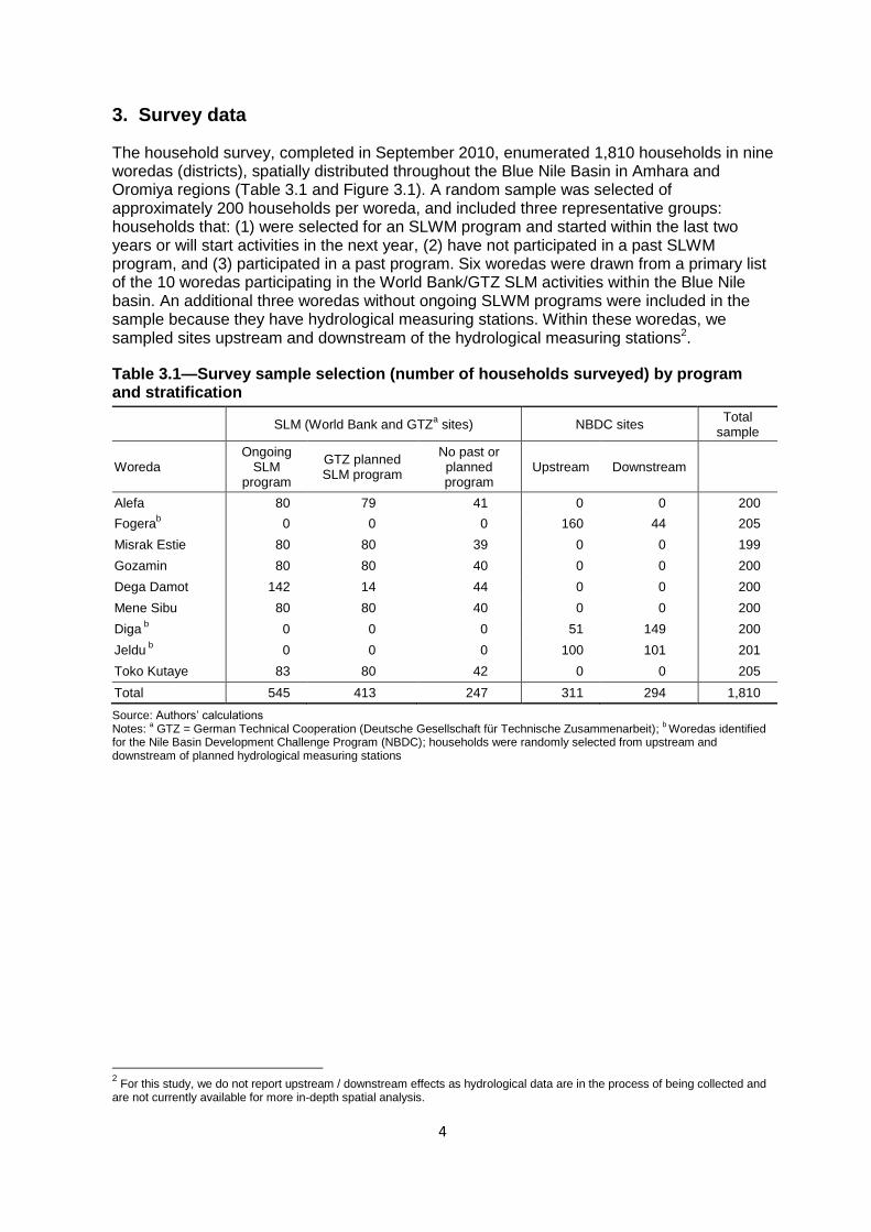
The household survey, completed in September 2010, enumerated 1,810 households in nine woredas (districts), spatially distributed throughout the Blue Nile Basin in Amhara and Oromiya regions (Table 3.1 and Figure 3.1). A random sample was selected of approximately 200 households per woreda, and included three representative groups: households that: (1) were selected for an SLWM program and started within the last two years or will start activities in the next year, (2) have not participated in a past SLWM program, and (3) participated in a past program. Six woredas were drawn from a primary list of the 10 woredas participating in the World Bank/GTZ SLM activities within the Blue Nile basin. An additional three woredas without ongoing SLWM programs were included in the sample because they have hydrological measuring stations. Within these woredas, we sampled sites upstream and downstream of the hydrological measuring stations2.

Table 3.1—Survey sample selection (number of households surveyed) by program and stratification

SLM (World Bank and GTZa sites) NBDC sites

Total sample

Woreda Ongoing

SLM program

GTZ planned SLM program

No past or planned program

Upstream Downstream

Alefa 80 79 41 0 0 200

Fogerab 0 0 0 160 44 205

Misrak Estie 80 80 39 0 0 199

Gozamin 80 80 40 0 0 200

Dega Damot 142 14 44 0 0 200

Mene Sibu 80 80 40 0 0 200

Diga b

0 0 0 51 149 200

Jeldu b

0 0 0 100 101 201

Toko Kutaye 83 80 42 0 0 205

Total 545 413 247 311 294 1,810

Source: Authors’ calculations Notes:

a GTZ = German Technical Cooperation (Deutsche Gesellschaft für Technische Zusammenarbeit);

b Woredas identified

for the Nile Basin Development Challenge Program (NBDC); households were randomly selected from upstream and downstream of planned hydrological measuring stations

2 For this study, we do not report upstream / downstream effects as hydrological data are in the process of being collected and

are not currently available for more in-depth spatial analysis.

5

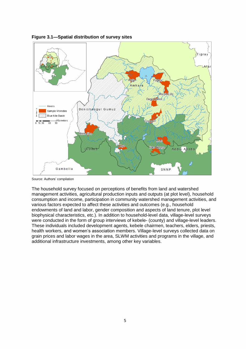
Figure 3.1—Spatial distribution of survey sites

Source: Authors’ compilation

The household survey focused on perceptions of benefits from land and watershed management activities, agricultural production inputs and outputs (at plot level), household consumption and income, participation in community watershed management activities, and various factors expected to affect these activities and outcomes (e.g., household endowments of land and labor, gender composition and aspects of land tenure, plot level biophysical characteristics, etc.). In addition to household-level data, village-level surveys were conducted in the form of group interviews of kebele- (county) and village-level leaders. These individuals included development agents, kebele chairmen, teachers, elders, priests, health workers, and women’s association members. Village-level surveys collected data on grain prices and labor wages in the area, SLWM activities and programs in the village, and additional infrastructure investments, among other key variables.

6

4. Household characteristics and perception of SLWM structures

A primary purpose of the SLWM household survey was to better understand the characterizations, constraints, and coping strategies of farmers within the context of longer term agricultural planning objectives. We find that public investments in SLWM are in line with constraints identified by surveyed households. The most common public SLWM infrastructures built in each of the villages focused on erosion mitigation and water conservation, such as check dams, trenches, tree planting, and terracing (Figure 4.1). When households were asked about past shocks, farmers reported that, on average, drought, hailstorms, and excess rain or flooding affected 48, 32, and 30 percent of farmer’s agricultural output, respectively. The survey further queried farmers regarding the most successful SLWM activity that had been implemented in the village; 34 percent of farmers identified stone terraces as the most successful project, while soil bunds and check dams were ranked most successful by 29 and 11 percent of households, respectively.

For the most part, SLWM program management, training, and information sharing (as well as other agricultural assistance) is organized and disseminated by development agents3 within the kebele (county). When asked how farmers received information and advice on how to construct bunds or terraces, 86 percent of respondents reported interacting with a development agent, while only 4 and 3 percent of households, respectively, received information from friends or neighbors. Similarly, over 90 percent of farmers who obtained assistance with improved seeds, fertilizer, and marketing identified development agents as the primary information provider.

Figure 4.1—SLWM activities implemented in the village (percent of total households)

Source: Authors’ calculations

When assessing the degree to which community members adopted sustainable land management measures beyond that of community-led projects, the survey asked a series of questions pertaining to private investments (land and labor) on agricultural land. Responses varied dramatically by woreda, and by previous exposure to an SLWM program. For example, only 2 percent of respondents from Jeldu woreda implemented SLWM activities4 on their own land, but 40 percent identified erosion as a concern on private agricultural lands

3

In an attempt to provide information, training, demonstrations, and advice on agricultural activities, farmer training centers were constructed at the kebele level. These training centers are staffed by three development agents who have graduated and/or interned at an Agricultural Technical and Vocational Education and Training (ATVET) college. 4 SLWM activities include building irrigation well, irrigation canal, and/or private pond; leveling land or clearing stones;

constructing stone terrace, soil bunds, check dam, drainage ditch, trenches, fences or water harvesting structures; planting trees, grass strips, live fence / barrier, or agroforestry activities; and gully rehabilitation

0

5

10

15

20

25

7

(Table 4.1). Jeldu woreda has received very little SLWM support programs, and thus zero respondents worked on a previous public SLWM program (as compared to the sample average of 36 percent participation in a public program). In comparison 82 and 54 percent of respondents in Dega Damot and Fogera, respectively, reported implementing SLWM on their private land, while 43 percent of respondents in each woreda also participated in a past community program to build SLWM structures.

Table 4.1—Households using SLWM on private land

Woreda Percent

of woreda

Year of first community

program

Most common activity on private

land (percent)*

Alefa 50% 1990 soil bund (64.2)

Fogera 54% 1983 stone terrace (65.8)

Misrak Estie 54% 1977 stone terrace (36.1)

Gozamin 21% 1988 soil bund (40.9)

Dega Damot 82% 1986 soil bund (42.8)

Mene Sibu 7% 1992 soil bund (89.8)

Diga 32% 2000 irrigation canal (2.9)

Jeldu 2% na stone terrace (24.0)

Toko Kutaye 79% 1989 soil bund (33.7)

Source: Authors’ calculations Note: *We do not report drainage ditch because activity and definition varied dramatically by household

Although the survey sites are focused within the Blue Nile Basin and primarily within the highland regions of Ethiopia, agricultural production strategies differ among woredas. Maize and teff are common crops on many sites. Within the sample, 64 percent of farmers grow maize on a portion of their land; more than half of the farmers surveyed grow teff (55 percent); and over 40 percent of farmers grow barley and wheat. However, due to high altitude constraints, Dega Damot woreda focuses on barley, wheat, and potato production, while Jeldu woreda (reported to have irrigation potential) focuses on barley and wheat production. Although a majority of production is confined to the major highland crops, substantial diversity exists across woredas in terms of production patterns and agricultural activity which has implications for income generation and production value.

The mean value of production also varies dramatically by site. Fogera woreda, with almost half of its production area (47 percent) dedicated to teff (a high value crop used to make injera in Ethiopia), and Diga woreda, known as a fertile maize production area, enjoy relatively high values of production of 11,835 and 13,098 birr per household per year respectively5 (Table 4.2). Average farm size also varies by woreda, and is larger in Fogera and Jeldu (1.44 and 1.98 hectares, respectively). Diga woreda has the highest production value, with the largest average farm size in the sample and focuses predominantly on maize production (64 percent of agricultural area). The fact that agricultural income is different from expenditures in some woredas may be driven by a number of factors such as varying saving rates, non-farm income, market price transmission and market accessibility, as well as systematic under-reporting of income6.

5 These shares take into account the five major cereals (teff, maize, sorghum, barley, wheat) and potatoes.

6 There is substantial literature regarding under-reporting of income, examples of such are Clotfelter (1983), Slemrod (1985),

and Bound et al. (2001).

8

Table 4.2—Production patterns by woreda

District (Woreda)

Mean Value Production (Birr/HH/yr)

Mean Total Expenditure (Birr/HH/yr)

Production / Expenditure

Mean Total Expenditure

(Dollars/HH/yr)*

Farm Size (hectares / person)

Major crops (percent of

cultivated area)

Alefa 7,741 12,171 0.64 869 0.99 Maize (36%),

Teff (32%)

Fogera 11,835 9,565 1.24 683 1.44 Teff (47%),

Maize (41%)

Misrak Estie 4,892 13,237 0.37 946 1.32 Teff (31%),

Wheat (29%)

Gozamin 9,263 9,751 0.95 697 1.08 Teff (42%),

Wheat (24%)

Dega Damot 4,490 9,047 0.5 646 1.00 Barley (33%), Wheat (28%),

Potatoes (21%)

Mene Sibu 6,254 8,267 0.76 591 1.58 Maize (50%),

Sorghum (25%), Teff (24%)

Diga 13,098 11,195 1.17 800 2.48 Maize (64%),

Sorghum (26%)

Jeldu 7,569 14,229 0.53 1016 1.98 Barley (35%), Wheat (21%)

Toko Kutaye 7,505 16,935 0.44 1210 2.10 Teff (38%),

Wheat (20%), Barley (19%)

Average 8,072 11,600 0.73 829 1.55 -

Source: Authors’ calculations Note: * Exchange rate in 2009/2010 was 14 birr to the US dollar

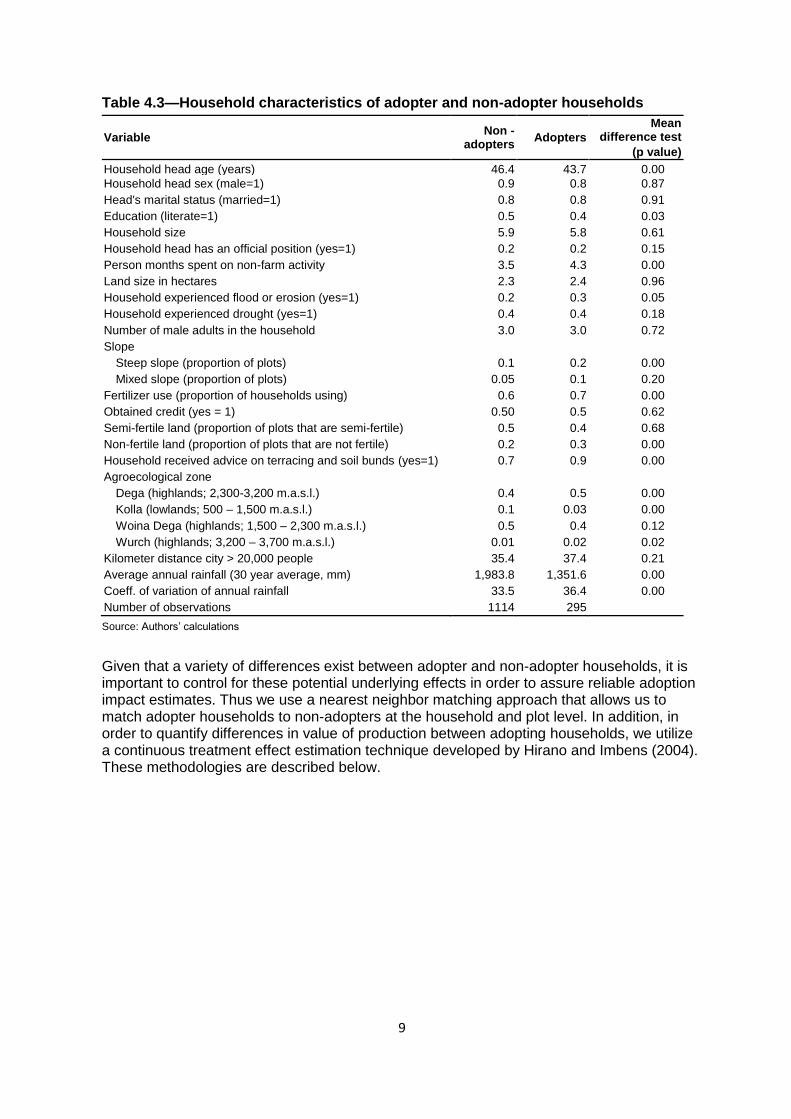
In addition to variations across woredas in terms of agricultural production and land endowments, significant differences exist between households that adopt SLWM and households that do not adopt on their private land. Households that adopted SLWM within the last 15 years (since 1994) received less rainfall on average, endured greater variation of rainfall, and reported experiencing erosion in the past (Table 4.3). In addition, adopter households tend to farm land with poorer reported soil fertility and steeper slopes. Significant differences in household head characteristics between adopters and non-adopters (age, education, and household size) also exist. Finally, a significantly higher percentage of adopting households use fertilizer on their agricultural land, and have received targeted advice on constructing and maintaining terracing and bund structures on private land.

9

Table 4.3—Household characteristics of adopter and non-adopter households

Variable Non -

adopters Adopters

Mean difference test

(p value)

Household head age (years) 46.4 43.7 0.00

Household head sex (male=1) 0.9 0.8 0.87

Head's marital status (married=1) 0.8 0.8 0.91

Education (literate=1) 0.5 0.4 0.03

Household size 5.9 5.8 0.61

Household head has an official position (yes=1) 0.2 0.2 0.15

Person months spent on non-farm activity 3.5 4.3 0.00

Land size in hectares 2.3 2.4 0.96

Household experienced flood or erosion (yes=1) 0.2 0.3 0.05

Household experienced drought (yes=1) 0.4 0.4 0.18

Number of male adults in the household 3.0 3.0 0.72

Slope

Steep slope (proportion of plots) 0.1 0.2 0.00

Mixed slope (proportion of plots) 0.05 0.1 0.20

Fertilizer use (proportion of households using) 0.6 0.7 0.00

Obtained credit (yes = 1) 0.50 0.5 0.62

Semi-fertile land (proportion of plots that are semi-fertile) 0.5 0.4 0.68

Non-fertile land (proportion of plots that are not fertile) 0.2 0.3 0.00

Household received advice on terracing and soil bunds (yes=1) 0.7 0.9 0.00

Agroecological zone

Dega (highlands; 2,300-3,200 m.a.s.l.) 0.4 0.5 0.00

Kolla (lowlands; 500 – 1,500 m.a.s.l.) 0.1 0.03 0.00

Woina Dega (highlands; 1,500 – 2,300 m.a.s.l.) 0.5 0.4 0.12

Wurch (highlands; 3,200 – 3,700 m.a.s.l.) 0.01 0.02 0.02

Kilometer distance city > 20,000 people 35.4 37.4 0.21

Average annual rainfall (30 year average, mm) 1,983.8 1,351.6 0.00

Coeff. of variation of annual rainfall 33.5 36.4 0.00

Number of observations 1114 295

Source: Authors’ calculations

Given that a variety of differences exist between adopter and non-adopter households, it is important to control for these potential underlying effects in order to assure reliable adoption impact estimates. Thus we use a nearest neighbor matching approach that allows us to match adopter households to non-adopters at the household and plot level. In addition, in order to quantify differences in value of production between adopting households, we utilize a continuous treatment effect estimation technique developed by Hirano and Imbens (2004). These methodologies are described below.

10

5. Methodology

Three primary questions are explored in this paper. First, we calculate the impact that SLWM has on the value of production and livestock holdings for adopting households compared to non-adopting households and, at plot level, plots that received investments versus those that did not. In doing so, we use a probit regression technique that provides insight on which type of household or plot is more likely to adopt or receive investment and maintain SLWM structures on private land. Second, we estimate the marginal benefit of maintaining SLWM infrastructure from one year to the next, as well as how long farmers must maintain SLWM structures in order to experience a benefit. Finally, we construct a benefit cost analysis taking into account the extra value benefit from increased production due to investment and maintenance of SLWM in comparison to initial construction and ongoing maintenance costs in terms of labor at the household level.

5.1. Nearest neighbor matching

In order to evaluate household determinants and impact of adoption, we encounter a common problem that any non-experimental evaluation faces, which is that of assigning causation and calculating treatment effects. Many past studies discuss the inherent problem of comparing a treatment group to a non-experimental control group whereby causal effect may be biased due to self-selection or methodical assignment of treatment groups by program management decisions or funding mechanisms and priorities. In order to control for such bias, given that a variety of SLWM programs were implemented in the past (with the most recent investments implemented by the World Bank and GTZ in 2008–2011 (2000/2001–2003/2004 Ethiopian calendar)), we estimate the average treatment effect on the treated (ATT), using the nearest-neighbor matching method (NNM)7 which matches adopters and non-adopter/control households based on observable characteristics and calculates the mean difference in outcomes across the two groups. Thus, the control group is matched on the probability (propensity score) of adopting given a set of observable characteristics from a probit regression. (Quisumbing et al. 2011 provide a comprehensive overview of NNM).

When matching adopter households that implemented and sustained SLWM on their private land versus non-adopter households that did not construct SLWM structures, we use the following definitions for adopter households: (1) the household implemented and continues to maintain terraces, stone/soil bunds, or check dams8 on their private land and (2) the household constructed these structures on at least 1/3 of their total agricultural land holdings9. Using this definition of adoption, we estimate a propensity score that is based on a probit regression (at the household level) of the probability of adopting SLWM given observed household and village level characteristics10. The sample is then balanced by calculating and verifying that the means of the observed characteristics included in the probit model are similar for adopter households as compared to non-adopters. Individual adopter households are then paired with non-adopter households when their respective observable characteristics are similar, as determined by a weighted average of the distance between values of the observed characteristics. Comparison households with propensity scores that are nearest to adopter households receive the highest weights and are matched accordingly.

7 The NNM method is similar to propensity score matching with the key differences being that NNM matches treated

households to comparison households using a weighted approach that determines a multidimensional metric across all covariates. The NNM approach is nonparametric and relies on analytical standard errors as opposed to PSM which employs probit or logit models to estimate the propensity scores. 8 Stone terraces, bunds, and check dams were identified by the entire sample as the most important SLWM infrastructure

implemented—see Figure 6.1. 9

If the household built an SLWM structure on a plot, the entire plot area is assumed to be under SLWM 10

Methodology description is adapted from Kumar and Quisumbing (2010)

11

We then compare average outcomes of the adopter households with the matched non-adopter/comparison households.

Heckman, Ichimura, and Todd (1997, 1998) underline the importance of a comparable group of comparison observations, as well as comprehensive survey data that target characteristics correlated with the tested technology and outcome variables in order to assure reliable estimates of program impact using matching methods. Given that the data used in this study comprises the baseline survey for the current programs being implemented (2008–2011), we stratified the sample in order to allow for robust estimates of a single-difference in outcomes analysis by matching (which can later be compared to future survey panel data analysis estimating difference in difference outcomes). Thus, we randomly sample from villages and households that are within the same woreda as the programmed villages, but are/will not receive a program in the foreseeable future.

Once a balanced sample is achieved and trimmed (we trim 5 percent of the sample from the top and bottom of the non-participant distribution in terms of propensity scores in order to assure comparisons over the same propensity score range), we proceed to estimate the average treatment effect of adopting SLWM on private land using NNM. NNM allows us to identify and construct a suitable comparison group of households whose average outcomes provide an unbiased estimate of the result that adopter households would have if they had chosen not to adopt. Each adopter household is matched to a non-adopter household with its closest propensity score (allowing for five nearest neighbors in terms of absolute difference in propensity scores). Thus, for each household i, there are two potential outcomes: adoption or no adoption. We denote adopters as Ai(1) and non-adopters as Ai(0), whereby the impact of adopting SLWM is the difference in outcome between adopters and non-adopters: Δ = A1 – A0

11. However, A1 or A0 for each household is observed uniquely

given the unknown of the counterfactual. Thus, when D is an indicator variable equal to 1 if the household adopts SLWM and 0 if the household is a non-adopter, we find that the average impact of adopting —the average impact of the treatment on the treated (ATT)—is defined as the following when X is a vector of control variables:

Two key results are derived from the above analysis. The first result is obtained from estimating the probit model which predicts the probability of each household adopting SLWM. This allows us to identify specific household level determinants of adoption and participation in SLWM activities, controlling for initial characteristics and endowments. The probit model is also integral to obtaining a balanced sample of adopter and non-adopter observations, in order to estimate impact. The second analysis estimates the average effect or impact of SLWM participation. In this case, we are interested in measuring how total agricultural value of production and livestock holdings differ between households that implement SLWM on private land and those that do not adopt such structures. Results of these analyses are discussed in section 6.

5.2. Dose response and treatment effect estimates

When setting the model to estimate the continuous treatment effect, we follow Hirano and Imbens (2004) in their work on propensity score matching with continuous treatment. In this

study, we consider a set of plots indexed by i where i=1,…,N. Letting t T where t is the level of treatment defined as the number of years households have been implementing soil bunds, terraces, or check dams on their specific plots, there is a certain level of potential

outcome,

( )iY t capturing the response to a level of treatment. In our particular case we

11

The methodology explained here follows Abadie and Imbens (2002).

12

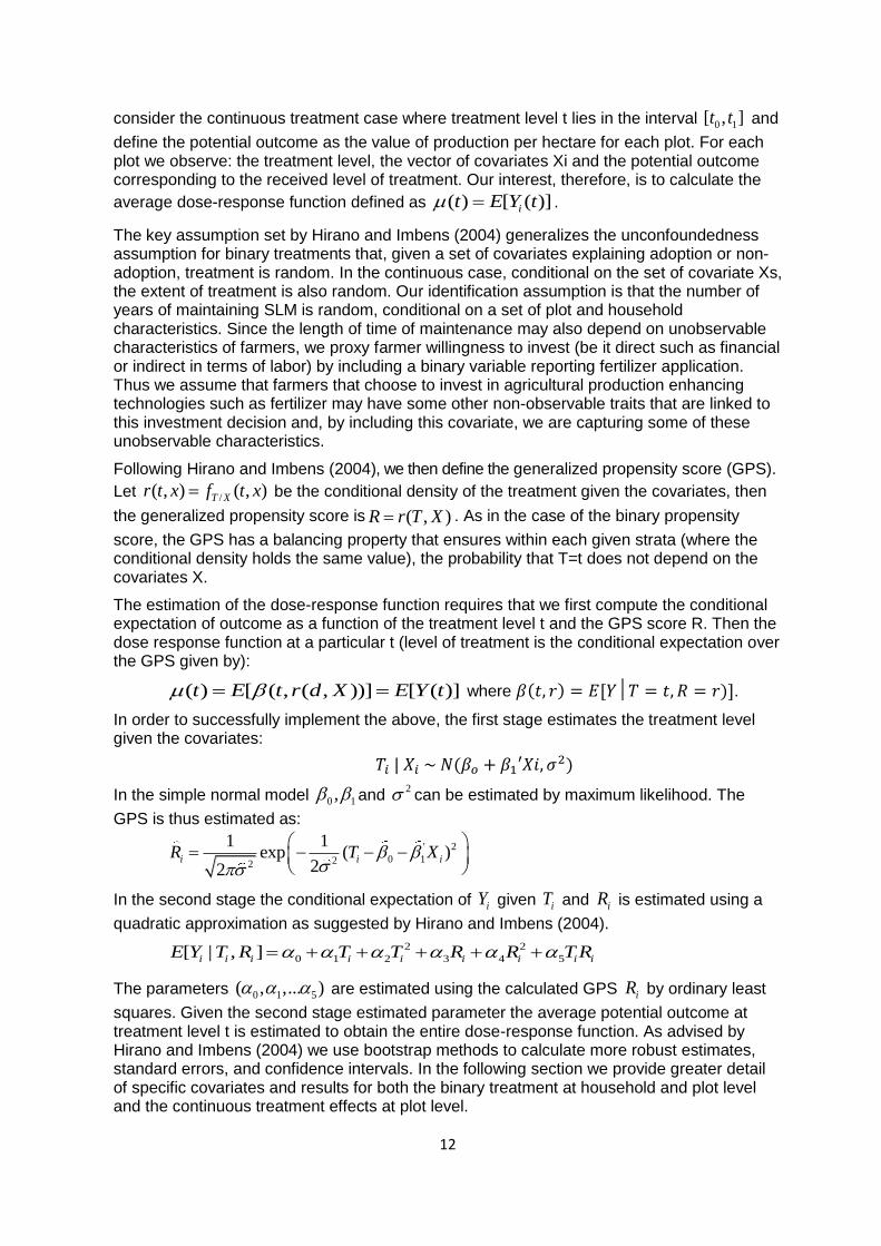
consider the continuous treatment case where treatment level t lies in the interval 0 1[ , ]t t and

define the potential outcome as the value of production per hectare for each plot. For each plot we observe: the treatment level, the vector of covariates Xi and the potential outcome corresponding to the received level of treatment. Our interest, therefore, is to calculate the

average dose-response function defined as ( ) [ ( )]it E Y t .

The key assumption set by Hirano and Imbens (2004) generalizes the unconfoundedness assumption for binary treatments that, given a set of covariates explaining adoption or non-adoption, treatment is random. In the continuous case, conditional on the set of covariate Xs, the extent of treatment is also random. Our identification assumption is that the number of years of maintaining SLM is random, conditional on a set of plot and household characteristics. Since the length of time of maintenance may also depend on unobservable characteristics of farmers, we proxy farmer willingness to invest (be it direct such as financial or indirect in terms of labor) by including a binary variable reporting fertilizer application. Thus we assume that farmers that choose to invest in agricultural production enhancing technologies such as fertilizer may have some other non-observable traits that are linked to this investment decision and, by including this covariate, we are capturing some of these unobservable characteristics.

Following Hirano and Imbens (2004), we then define the generalized propensity score (GPS).

Let /( , ) ( , )T Xr t x f t x be the conditional density of the treatment given the covariates, then

the generalized propensity score is ( , )R r T X . As in the case of the binary propensity

score, the GPS has a balancing property that ensures within each given strata (where the conditional density holds the same value), the probability that T=t does not depend on the covariates X.

The estimation of the dose-response function requires that we first compute the conditional expectation of outcome as a function of the treatment level t and the GPS score R. Then the dose response function at a particular t (level of treatment is the conditional expectation over the GPS given by):

( ) [ ( , ( , ))] [ ( )]t E t r d X E Y t where .

In order to successfully implement the above, the first stage estimates the treatment level given the covariates:

In the simple normal model 0 1, and 2 can be estimated by maximum likelihood. The

GPS is thus estimated as:

' 2

0 122

1 1exp ( )

22i i iR T X

In the second stage the conditional expectation of iY given iT and iR is estimated using a

quadratic approximation as suggested by Hirano and Imbens (2004).

2 2

0 1 2 3 4 5[ | , ]i i i i i i i i iE Y T R T T R R T R

The parameters 0 1 5( , ,... ) are estimated using the calculated GPS iR by ordinary least

squares. Given the second stage estimated parameter the average potential outcome at treatment level t is estimated to obtain the entire dose-response function. As advised by Hirano and Imbens (2004) we use bootstrap methods to calculate more robust estimates, standard errors, and confidence intervals. In the following section we provide greater detail of specific covariates and results for both the binary treatment at household and plot level and the continuous treatment effects at plot level.

13

6. Results

6.1. Nearest neighbor matching

Unlike technologies such as fertilizer or improved seeds that reap increased yields within a season or year, benefits realized from constructing SLWM structures may accrue over longer time horizons. Nutrient and soil depletion is acute in areas of Ethiopia, and repletion is a multi-stage / year process. Given this lag, we designed the household survey to take into account past interventions that farmers completed and asked the length of time that the household maintained the infrastructure. Thus, we identify adopter households as those that constructed terraces, bunds, or check dams (identified as the most successful SLM interventions) on at least 1/3 of their land by at least 1992 or onwards and continued to maintain these structures until the date of the survey in 2010. By this definition, 24 percent of the households in the sample are adopter households.

We first evaluate overall effects by matching all adopter households from 1992 onwards with non-adopter households to identify determinants of adoption from the probit model estimations, as well as evaluate any impact for overall program adoption regardless of the date of implementation. Then, in order to take into account the hypothesized lag time for benefit realization, we split the adopter sample by reported date that structures were first built on plots. We separately evaluate adopters that built infrastructure during the initial period (1992–2002) and then again for the more recent implementation period (2003–2009).

We choose to analyze by two major implementation periods following spikes and drops in SLWM activity over the last two decades, as reflected in the data (Figure 6.1). In addition, although data exist on farmers implementing earlier than 1992, we choose to start the analysis here for several reasons. First, we choose a date after the Derg Regime12 in order to not confound results with major political upheavals and policy change. Second, less than 2 percent of the total sample implemented structures in any given year prior to 1992, and less than 1 percent of plots in the sample implemented SLWM on their private land in 1992 (which created a natural baseline of minimal activity). Note that in our sample, the largest spike of investment is in 199613. Investments then fall off dramatically until the most recent investment effort which started in 2007 (Figure 6.1). Thus we are able to analyze two relatively more intensive periods of SLWM implementation. Each of these analyses requires separate NNM estimations, but we maintain the same variables for each analysis, and in each analysis we maintain a balanced sample.

12

An intense power struggle characterized the years between 1974 and 1977 and Mengistu became the Derg leader in February 1977. Chronic food insecurity characterized the 1980s; with a famine in 1984. The regime collapsed May 28, 1991 (Rashid et al. 2009). 13

Several large SLWM programs were initiated in 1996 after usufruct land tenure laws were publicly announced. This included projects led by the NGO SOS Sahel in North Wollo zone near Fogera woreda in 50 sites; Sida Amhara Rural Development Programme (SARDP) program in East Gojjam and South Wollo (Gozamin and Misrak Este woredas); and Birbirssa na Cherecha Development Programme (BCDP) that focused on bund and terrace construction in West Shewa (Toko Kutaye woreda) from 1996 to 2004.

14

Figure 6.1—Percent of total plots under SLWM on private land (1937–2009)

Source: Authors’ calculations

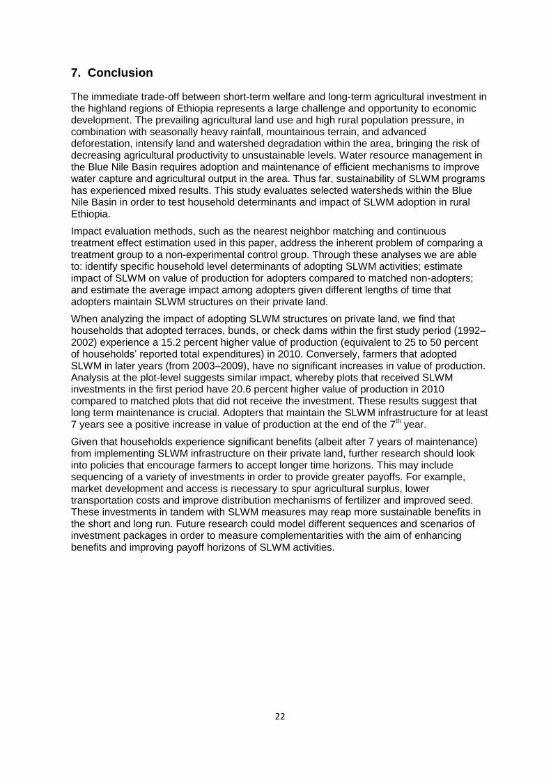
6.1.1. Determinants of adoption

The household probit model that is used to match adopter and non-adopter households reveals interesting information about household probability of SLWM adoption on private land. It is important to note that causation of whether to adopt or not cannot be attained from the probit regression, but rather these results describe linkages between adopters and non-adopters which suggest correlation with SLWM investment among households. The following presents a selection of the household level probit regression results (complete results from the household and plot level probit can be found in Appendix Tables A.1 and A.2). The share of non-fertile lands is significantly different between adopters and non-adopters, suggesting that households with a greater percentage of land on steep slopes or reported as semi-fertile and non-fertile, is correlated with SLWM investment on their private land. In addition to biophysical constraints, past experience of flood or erosion is significantly different between adopters and non-adopters suggesting that households that previously experienced flood or erosion may be more inclined to adopt SLWM to insure against similar future occurrences.

Remoteness has a significant but small negative correlation with household probability of adopting SLWM. There may be several reasons for this relationship. First, if farmers do not see a marketable outlet for increased production, they may be less willing to implement structures that could increase yields to the point where prices are driven down given thin, local markets. In addition, the agricultural extension programs and placement of development agents in remote areas may have lagged behind areas that are better connected to market centers, and thus remote households may not have received necessary or frequent information or training.

In addition, we include fertilizer application as a matching binary variable in order to proxy willingness to invest in technologies / innovation to increase output. We find that the decision to apply fertilizer significantly differs between adopters and non-adopters suggesting a positive correlation with adoption decision and willingness to invest in other agricultural enhancing technologies. Given that in the next stage of matching, a major assumption is that we are able to match based on observables, we also argue that fertilizer application assists

0

2

4

6

8

10

12

14

16

18

20

15

in controlling for unobservables that may be present such as technology uptake and willingness to invest14.

Finally, we observe that households adopted SLWM strategies in varying past years. It is important that the probit model discussed above includes covariates that would not have changed after adopting SLWM. For example, we include total landholding size, biophysical characteristics of agricultural land such as soil quality and slope, and household head characteristics which are less likely to change over the study period. In order to further control for endogeneity, we do not match adopter and non-adopter households based on assets which may have been affected by successful or unsuccessful investment in SLWM adoption (i.e. changes in livestock holdings or variables that proxy income).

6.1.2. Impacts of adoption

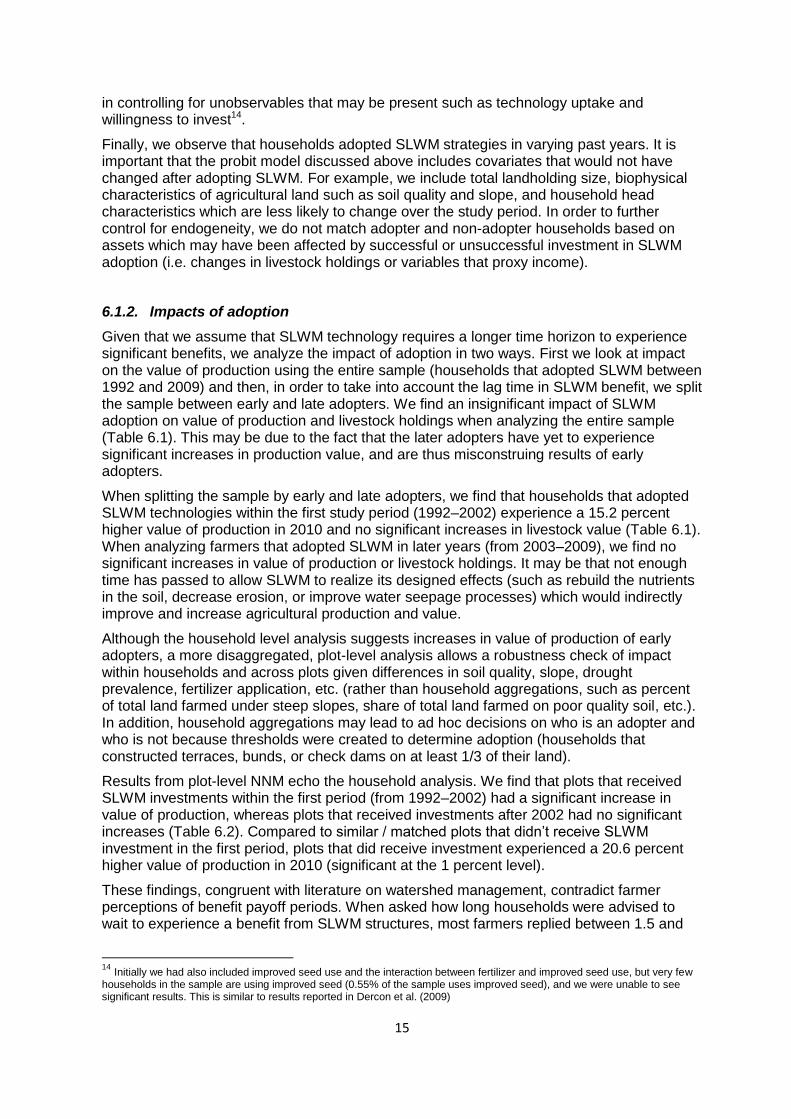
Given that we assume that SLWM technology requires a longer time horizon to experience significant benefits, we analyze the impact of adoption in two ways. First we look at impact on the value of production using the entire sample (households that adopted SLWM between 1992 and 2009) and then, in order to take into account the lag time in SLWM benefit, we split the sample between early and late adopters. We find an insignificant impact of SLWM adoption on value of production and livestock holdings when analyzing the entire sample (Table 6.1). This may be due to the fact that the later adopters have yet to experience significant increases in production value, and are thus misconstruing results of early adopters.

When splitting the sample by early and late adopters, we find that households that adopted SLWM technologies within the first study period (1992–2002) experience a 15.2 percent higher value of production in 2010 and no significant increases in livestock value (Table 6.1). When analyzing farmers that adopted SLWM in later years (from 2003–2009), we find no significant increases in value of production or livestock holdings. It may be that not enough time has passed to allow SLWM to realize its designed effects (such as rebuild the nutrients in the soil, decrease erosion, or improve water seepage processes) which would indirectly improve and increase agricultural production and value.

Although the household level analysis suggests increases in value of production of early adopters, a more disaggregated, plot-level analysis allows a robustness check of impact within households and across plots given differences in soil quality, slope, drought prevalence, fertilizer application, etc. (rather than household aggregations, such as percent of total land farmed under steep slopes, share of total land farmed on poor quality soil, etc.). In addition, household aggregations may lead to ad hoc decisions on who is an adopter and who is not because thresholds were created to determine adoption (households that constructed terraces, bunds, or check dams on at least 1/3 of their land).

Results from plot-level NNM echo the household analysis. We find that plots that received SLWM investments within the first period (from 1992–2002) had a significant increase in value of production, whereas plots that received investments after 2002 had no significant increases (Table 6.2). Compared to similar / matched plots that didn’t receive SLWM investment in the first period, plots that did receive investment experienced a 20.6 percent higher value of production in 2010 (significant at the 1 percent level).

These findings, congruent with literature on watershed management, contradict farmer perceptions of benefit payoff periods. When asked how long households were advised to wait to experience a benefit from SLWM structures, most farmers replied between 1.5 and

14

Initially we had also included improved seed use and the interaction between fertilizer and improved seed use, but very few households in the sample are using improved seed (0.55% of the sample uses improved seed), and we were unable to see significant results. This is similar to results reported in Dercon et al. (2009)

16

2.5 years (Table 6.3). Given the contradiction between farmer perception of benefit timing and this analysis, there may be a mismatch of expectations between program or information providers and SLWM adopters. However, it is important to acknowledge that benefits can be defined beyond that of increased value of production or livestock holdings. For example, gully rehabilitation improves livestock herding expansion and transportation as deep furrows are filled and access becomes easier and more efficient across terrain.

Table 6.1—Average household-level impact of SLWM adoption (single difference estimates)

Outcome variable ATT Observations

1992–2002 (1985–1995 E.C.)

Value of agricultural production 0.152** 1373

(0.071)

Livestock value (in Birr) -0.429 1318

(.100)

2003–2009 (1996–2002 E.C.)

Value of agricultural production -0.015 1397

(0.062)

Livestock Value (in Birr) -0.158 1327

(0.095)

1992–2009 (1985–2002 E.C.)

Value of agricultural production 0.022 1397

(0.056)

Livestock value (in Birr) -0.085 1213

(0.072)

Source: Authors’ calculations Note: ATT = average treatment effect on the treated; * and ** are significance level at 10% and 5%, respectively

Table 6.2—Average plot-level impact of SLWM adoption (single difference estimates)

Outcome variable: Value of agricultural production

ATT Observations

1992–2002 (1985–1995 E.C.) 0.206*** 10108

(0.035)

2003–2009 (1996–2002 E.C.) -0.025 10108

(0.030)

1992–2009 (1985–2002 E.C.) 0.0602 10108

(0.025)

Source: Authors’ calculations Note: ATT = average treatment effect on the treated; *** significance level at 1%; standard errors are in brackets

17

Table 6.3—Average number of years the information providers report to benefit from SLWM adoption

Woreda

Construction of bunds

or terraces Building drainage

Irrigation/ water harvesting

system

Alefa 2.38 2.10 1.29

Fogera 2.12 2.33 1.38

Misrak Estie 1.59 1.35 1.23

Gozamin 1.70 1.38 1.17

Dega Damot 2.12 1.72 1.60

Mene Sibu 1.74 1.47 1.56

Diga 1.17 1.80 1.14

Jeldu 1.50 1.50 2.00

Toko Kutaye 3.98 3.80 1.33

Source: Authors’ calculations

6.2. Dose response and continuous treatment effect estimation results

6.2.1. Payoff period

In order to better evaluate payoff period and marginal effects of SLWM adoption on private land, we employ a methodology of continuous treatment estimation as proposed by Hirano and Imbens (2004). Thus, we are able to estimate, among adopters of the technology, how plot level value of production varies according to years that SLWM is maintained. In this case, adoption is evaluated at the plot level because households implement SLWM on diverse plots in different years. We then calculate the difference of impact based on the length of time that terraces, bunds, or check dams have been constructed and maintained on a specific plot.

For the first stage regression, we estimate the conditional distribution of the number of years a SLWM structure is maintained given a set of covariates (Appendix Table A.3). We estimate a treatment level (defined by number of years) in order to obtain a generalized propensity score (GPS) using plot-level and household characteristics. We then divide the treatment distribution by treatment level whereby we define three time intervals in years: [1,5], [6,10] and [11,15]. For each of these intervals, a group of observations is identified. There are 963, 563, and 603 observations in each group respectively.

For each of the covariates used in the first regression, we then test and confirm that the mean of one group is similar to the other two groups combined, and thus are able to satisfy the balancing property. Based on the suggestions of Hirano and Imbens (2004), who extended the concept of balancing in the binary treatment case, Table 6.4 is presented to explore whether the GPS actually balances the set of variables in the different intervals of the treatment level. The first three columns presented in the table test whether the covariates have the same mean for observations within the same treatment intervals using the raw data. Here we can see that the raw data are unbalanced for most of the covariates. In contrast, the last three columns are mean differences after adjusting for the GPS to see whether the covariates are better balanced when we condition on the estimated GPS. In comparing the two sets of results, we can clearly see that the covariates are better balanced after the GPS adjustment.

18

Table 6.4—Test for equality of means between treatment groups

Raw data

treatment terciles

Data adjusted by GPS treatment terciles

[1,5] [6,10] [11,15]

[1,5] [6,10] [11,15]

Household size -0.15* 0.00 0.19*

-0.11 -0.01 0.00

Education of head (literate=1) 0.01 -0.01 0.00

-0.01 -0.01 0.03

Fertilizer use (yes=1) -0.05** -0.01 0.06***

0.02 0.02 -0.02

Experienced flood/erosion (yes=1) -0.08*** -0.01 0.1***

-0.01 0.00 0.01

Age of household head -0.74 1.09* -0.14

-0.70 1.10 -0.36

Sex of household head 0.00 -0.01 0.01

0.01 -0.01 0.00

Slope of plot (steep=1) 0.02 -0.04** 0.02

0.01 -0.03 0.02

Soil quality

Semi-fertile (yes=1) 0.13*** 0.00 -0.16***

0.01 -0.03 0.01

Non fertile (yes=1) -0.02 -0.01 0.04**

-0.01 0.01 -0.01

Number of years village had program on bunds and terraces

0.45 0.19 -0.72**

0.01 0.08 0.54

Source: Authors’ calculations Note: GPS = generalized propensity score

After insuring that adjusting for the GPS improves the balance of the covariates across the treatment intervals, we proceed to the second-stage estimation of the model (second stage regression results are presented in Appendix Table A.4). We do not go into detail interpreting the second stage estimation given that these results do not have direct meaning on the impact analysis15. In other words, the estimated parameters are not used to make any suggestion on whether or not the treatment has significant impact on the potential outcome. Finally, the second stage regression function is averaged over the generalized propensity score function at each level of treatment (number of years that SLWM is sustained). We report the treatment effect function which is the derivative of the dose-response function, or the marginal effect of an additional year of maintenance of SLWM infrastructure.

Analysis suggests that maintenance of SLWM is crucial to reap significant benefits from investment. Adopters that maintain the SLWM infrastructure for at least 7 years see a positive increase in value of production at the end of the 7th year (Table 6.5 and Figure 6.2). For adopters that have maintained their infrastructure less than seven years, we do not see a statistically significant impact (we present the dose response function, including confidence intervals in Appendix A.5). This result may be due to a variety of reasons. According to other studies, land degradation in terms of nutrient and top soil loss is significant in the Ethiopian highlands (Yesuf et al. 2005). We expect that soil and water conservation structures—such as terraces, bunds, and check dams—would begin to slow this type of degradation in the initial years of maintenance, but nutrient build-up may take more time to show significant results on value of production. Although in initial years, impact analysis results are not significant (first 6 years of implementation), the negative marginal effect reported suggests that SLWM infrastructure may require a longer time horizon to slow degradation effects to a point where biophysical improvements (such as soil nutrients and water capture or storage) are realized to full potential. In addition, a package of conservation activities may be necessary in order to expedite benefits in terms of value of production. A study examining soil degradation and nutrient repletion on smallholder farms in Kenya found that fallow land alone did not overcome nitrogen deficiency after 8 seasons (Amadalo et al. 2003), but rather

15

According to Hirano and Imbens (2004), the parameters of the second-stage estimation do not have a direct meaning to the estimated coefficients in the model, rather satisfying the balancing property is the primary test whether the covariates introduce any bias.

19

a mix of strategies including organic and inorganic fertilizer application, intercropping, and fallowing were necessary to reap benefits.

Table 6.5—Marginal effect per extra year of maintenance

Level of treatment (years)

Marginal effect

1 -0.10 2 -0.08 3 -0.05 4 -0.03 5 -0.01 6 0.01 7 0.02* 8 0.04* 9 0.05*

10 0.06* 11 0.08* 12 0.09* 13 0.10* 14 0.12* 15 0.13*

Source: Authors’ calculations Note: * significant at least at the 10% level; we present the dose response function, including confidence intervals, in Appendix A.5

Figure 6.2—Treatment effect function given an additional year of investment

Source: Authors’ calculations

Not only is the marginal effect of adopting terraces, bunds, or check dams positive assuming maintenance for at least 7 years, but the marginal benefit increases at an increasing rate. Thus, for each additional year one sustains SLWM activities, the higher the gains in value of production. For example, if one sustains SLWM structures for 7 to 8 years, the value of production would increase by about 2 percent, whereas if a household continues to maintain SLWM for 14 to 15 years the expected value of production increases by 12 percent (Figure

Treatment range

with statistically

significant impact

20

6.2). Although the marginal benefit increases with each additional year that the structure is maintained, this increase becomes statistically insignificant after 15 years. In addition, there are minimal observations available for households that sustained SLWM for more than 12 years, and further investigation should be undertaken to understand the specific impacts of long-term maintenance. Assuming that nutrient repletion and erosion control is successful after long-term maintenance of SLWM structures, one would expect to see diminishing returns to such infrastructure as the necessary biophysical components are replaced. Further research over a longer time period may provide an estimated envelope of benefits and marginal returns. Although this envelope is yet to be established for farming systems within the Blue Nile basin, it is clear that SLWM adoption and maintenance does have a positive effect on value of production in the long run.

6.2.2. Cost benefit

The late onset of benefits suggested by the continuous treatment effect analysis (increase in value of production after 7 years) raises the question of whether these benefits outweigh initial investment costs and annual maintenance expenses in the long run. We compare the yearly marginal benefits with a rough estimation of costs, in terms of initial investment, labor, and time in order to evaluate net present value. We assume a constant, real recurrent labor cost for yearly maintenance of structures at 516 birr per year (which reflects the reported days and wage rate that investing farmers spend on SLWM activities per year). In addition, in order to evaluate net profitability of the investments, we use a range of estimated initial investment costs together with maintenance costs which are derived from the SLWM baseline survey. The analysis assumes that in the absence of adoption of SLWM technology, the value of production in all previous years was equal to the 2009 level (in real terms). Using a 5 percent discount rate, the net present value of production from 1992 to 2009 for non-adopters is 10,426 birr16.

It is important to note that the majority of SLWM investments occur between labor intensive seasons of planting or harvesting. This creates constrained wage employment opportunities, whereby labor supply exceeds that of wage employment possibilities in the village or nearby area, driving the wage rate down. Given the off-season nature of SLWM work, we present estimates of labor costs using both the actual market wage for construction and maintenance of structures and a shadow wage rate of 50 percent of the market wage.

Using a variety of estimated initial investment costs, we find that the increases in value of production do not always outweigh the discounted costs of the initial investment and maintenance (Table 6.6). In the first scenario, we assume a 5,000 (2009) birr initial investment (equivalent to approximately 10 times the marginal maintenance costs). Assuming the shadow wage rate is half that of market labor costs, results suggest that even by 2009, total discounted benefits do not exceed discounted costs. A second scenario assumes a 2,000 (2009) birr initial investment. In this scenario, benefits outweigh costs beginning in 2008 (benefit: cost ratio of 1.16), assuming a shadow wage rate factor of 50 percent. Finally, if we assume that the initial investments are fully subsidized (i.e. initial investment costs to the household are zero), but households still incur annual labor costs for maintenance, net benefits are positive beginning in 2006 and by 2009 are equal to 1.56 times that of costs. However, further work needs to focus on whether or not subsidies are the correct policy mechanism in this scenario.

16

We use a 5 percent discount rate in order to take into account the relatively high time value of money in rural Ethiopia, and opportunity cost of investing in other welfare enhancing activities such as reciprocal farming activities (debbo or wonfel), road maintenance, or other household projects.

21

Table 6.6—Cost-benefit of investing in SLWM infrastructure (1992–2009)

Initial investment cost (birr)

5000 2000 0

Shadow wage rate factor 1 0.5 1 0.5 1 0.5

NPV of Benefits 10,426 10,426 10,426 10,426 10,426 10,426

NPV of Costs 24,794 12,397 17,918 8,959 13,334 6,667

NPV Benefits / NPV Costs 0.42 0.84 0.58 1.16 0.78 1.56

First Year of Total Net Benefits > 0 NA NA NA 2008 NA 2006

First Year of MB > MC 2002 2000 2002 2000 2002 2000

Source: Authors’ calculations Notes: NPV = Net present value; MB = marginal benefits; MC = marginal costs; NA = not available

These rough results are consistent with other cost-benefit studies found in the literature, whereby benefits of soil and water conservation practices become tangible in the long run. Shiferaw and Holden (2001) analyzed experimental trials of bunds and terraces in west and east Amhara and found insufficient economic incentives for investment in such structures. Hengsdijk et al. (2005) underlined the tradeoffs of soil and conservation investments in Tigray region whereby bunds slightly increased crop productivity during drier periods when yields were low, but decreased productivity during moist seasons because overall cropped area was reduced for the construction of bunds. Regional differences are present, however. Gebremedhin et al. (1999) estimated a 50 percent rate of return on stone terraces based on experimental trials in central Tigray region. Yitbarek et al. (2010) implemented a more detailed cost-benefit analysis utilizing gully erosion costs, rehabilitation expenditure and rehabilitation benefits in four gully rehabilitation projects in Amhara region and found that two of the four programs showed monetary gains after 4 and 6 years respectively

Finally, it is often the case that larger projects that have an immediate cost (in this case, labor costs) at the beginning of the project rarely reap clear, quick benefits within a limited time frame. Given a higher discount rate whereby benefits further in the future are valued less than immediate benefits within the first several years of the project, the need to design incentive mechanisms to induce farmers to accept a longer planning horizon may be necessary. In addition, a mixture of strategies may reap quicker benefits. Physical SLWM measures may need to be integrated with soil fertility management (composting, cover crops, fertilizer application, etc.) and moisture management (mulching, deep plowing, etc.).

22

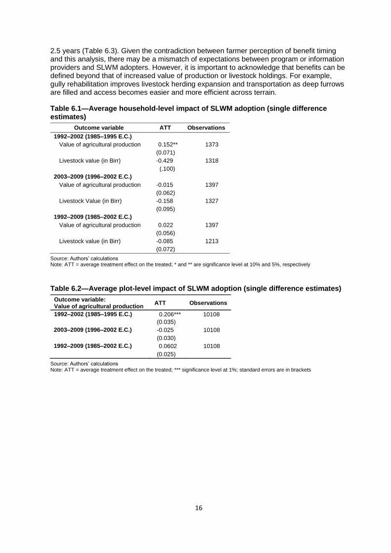
7. Conclusion

The immediate trade-off between short-term welfare and long-term agricultural investment in the highland regions of Ethiopia represents a large challenge and opportunity to economic development. The prevailing agricultural land use and high rural population pressure, in combination with seasonally heavy rainfall, mountainous terrain, and advanced deforestation, intensify land and watershed degradation within the area, bringing the risk of decreasing agricultural productivity to unsustainable levels. Water resource management in the Blue Nile Basin requires adoption and maintenance of efficient mechanisms to improve water capture and agricultural output in the area. Thus far, sustainability of SLWM programs has experienced mixed results. This study evaluates selected watersheds within the Blue Nile Basin in order to test household determinants and impact of SLWM adoption in rural Ethiopia.

Impact evaluation methods, such as the nearest neighbor matching and continuous treatment effect estimation used in this paper, address the inherent problem of comparing a treatment group to a non-experimental control group. Through these analyses we are able to: identify specific household level determinants of adopting SLWM activities; estimate impact of SLWM on value of production for adopters compared to matched non-adopters; and estimate the average impact among adopters given different lengths of time that adopters maintain SLWM structures on their private land.

When analyzing the impact of adopting SLWM structures on private land, we find that households that adopted terraces, bunds, or check dams within the first study period (1992–2002) experience a 15.2 percent higher value of production (equivalent to 25 to 50 percent of households’ reported total expenditures) in 2010. Conversely, farmers that adopted SLWM in later years (from 2003–2009), have no significant increases in value of production. Analysis at the plot-level suggests similar impact, whereby plots that received SLWM investments in the first period have 20.6 percent higher value of production in 2010 compared to matched plots that did not receive the investment. These results suggest that long term maintenance is crucial. Adopters that maintain the SLWM infrastructure for at least 7 years see a positive increase in value of production at the end of the 7th year.

Given that households experience significant benefits (albeit after 7 years of maintenance) from implementing SLWM infrastructure on their private land, further research should look into policies that encourage farmers to accept longer time horizons. This may include sequencing of a variety of investments in order to provide greater payoffs. For example, market development and access is necessary to spur agricultural surplus, lower transportation costs and improve distribution mechanisms of fertilizer and improved seed. These investments in tandem with SLWM measures may reap more sustainable benefits in the short and long run. Future research could model different sequences and scenarios of investment packages in order to measure complementarities with the aim of enhancing benefits and improving payoff horizons of SLWM activities.

23

Appendix

Appendix Table A.1—Household probit results: Determinants of SLWM adoption 1992–2009 (1985–2002 E.C.)

Variable dy/dx Std. Err.

HH head age (years) -0.013 ** (0.005)

HH head age sq. 0.000 * (0.000)

HH head sex (male=1) 0.011

(0.073)

Head's Marital status(married=1) 0.000

(0.069)

Household head has an official position (yes=1) -0.013

(0.031)

Person months spent on non-farm activity 0.003

(0.003)

Land size in hectares 0.019 ** (0.009)

Land size sq. -0.001

(0.000)

Household experienced flood and erosion (yes=1) 0.081 ** (0.034)

Household experienced drought (yes=1) 0.000

(0.030)

Number of male adults in the household 0.014

(0.012)

Household size -0.005

(0.008)

Slope (omitted=flat slope)

Steep slope (percentage of plots with steep slope) 0.159 *** (0.055)

Mixed slope (percentage of plots with mixed slope) 0.056

(0.077)

Fertilizer use (yes=1) 0.061 ** (0.028)

Education of HH head (literate=1) -0.016

(0.026)

Obtained credit (yes = 1) 0.004

(0.023)

Soil Quality (omitted=fertile land)

Semi-fertile land (percentage of plots that are semi-fertile) 0.066 *** (0.041)

Non fertile land (percentage of plots that are not fertile) 0.149 * (0.050)

Household received advice on terracing and bunds (yes=1) 0.084

(0.031)

Agroecological Zone (Omitted=Dega: mid-highlands 2,300-3,200m.)

Kolla (lowlands: 500 – 1,500m.) -0.181 *** (0.026)

Woina Dega (low-highlands: 1,500 – 2,300m.) -0.176 *** (0.052)

Wurch (upper-highlands: 3,200 – 3,700m.) 0.282 * (0.157)

Kilometer distance from city of at least 20,000 people -0.010 *** (0.003)

Annual rainfall (30 year average, mm) -0.001

(0.001)

Coef. of variation of annual rainfall 0.003

(0.003)

Woreda (omitted=Fogera)

Alefa 0.887 *** (0.074)

Misrak Estie -0.156 *** (0.039)

Gozamin -0.211 *** (0.017)

Dega Damot 0.289 * (0.170)

Mene Sibu 0.434 ** (0.201)

Toko Kutaye -0.207 *** (0.022)

Number of observations=1256

LR chi2(27) =253.59

Prob > chi2 =0

Pseudo R2 =0.2480

Source: Authors’ calculations Note: (*) dy/dx is discrete change of dummy variable from 0 to 1. *, **, and *** are significance level at 10%, 5% and 1% Dependent variable: Ln SLWM adoption on at least 1/3 of private land

24

Appendix Table A.2—Plot-level probit results: Determinants of SLWM adoption 1992–2009 (1985–2002 E.C.)

Variable dy/dx

Std. Err.

Age -0.002 *** 0.000

Sex -0.030 *** 0.011

Education (omitted > primary education

Primary education (yes = 1) 0.088 *** 0.020

No education((yes = 1) 0.122 *** 0.019

Fertilizer use 0.113 *** 0.008

Official 0.084 *** 0.010

Slope (omitted=steep slope)

Flat slope (percentage of plots with steep slope) -0.055 *** 0.011

Mixed slope (percentage of plots with mixed slope) -0.061 *** 0.014

Household experienced drought (yes=1) 0.048 *** 0.007

Soil Quality (omitted=fertile land)

Semi-fertile land (percentage of plots that are semi-fertile) 0.020 ** 0.010

Non fertile land (percentage of plots that are not fertile) 0.035 *** 0.007

Plot size > .25 hectares (yes=1) -0.031 *** 0.006

Number of obs=14316

Wald chi2(12)=510.26

Prob>chi2=0

Pseudo R2=0.039

Source: Authors’ calculations Note: (*) dy/dx is discrete change of dummy variable from 0 to 1. *, **, and *** are significance level at 10%, 5% and 1% Dependent variable: Plot receives SLWM (terracing, bunds, or check dams) investment (yes =1)

Appendix Table A.3—First stage Maximum likelihood estimates on treatment level

Coef. Std. Err.

Household size 0.00 0.01

Education of head (literate=1) 0.04 0.03

Fertilizer use (=1) -0.10 0.03

Experienced flood/erosion (=1) -0.16 0.03

Age of household head 0.00 0.00

Sex of household head 0.00 0.04

slope of plot (steep=1) 0.02 0.04

Soil quality 0.26 0.03

Semi-fertile (=1) 0.13 0.04

Non fertile (=1) 0.00 0.00

Number of years village had program on bunds and terraces 1.69 0.08

Source: Authors’ calculations

Appendix Table A.4—Second stage OLS Estimates on log of value of production

Coeff. Std. Err.

Time -0.12 0.06

Time_squared 0.01 0.00

Log(score) 1.93 0.90

Log (score)_squared -2.04 1.08

Time*score 0.05 0.05

_cons 8.16 0.20

Source: Authors’ calculations

25

Appendix A.5—Dose response function and Treatment effect function

7.5

88.5

9

E[lnvalu

epro

d(t

)]

0 5 10 15 20Treatment level

Dose Response Low bound

Upper bound

Confidence Bounds at .95 % levelDose response function = Linear prediction

Dose Response Function

-.2

-.1

0.1

.2.3

E[lnvalu

epro

d(t

+1)]

-E[lnvalu

epro

d(t

)]

0 5 10 15 20Treatment level

Treatment Effect Low bound

Upper bound

Confidence Bounds at .95 % levelDose response function = Linear prediction

Treatment Effect Function

26

References

Abadie, A., and G. W. Imbens. 2002. Simple and bias-corrected matching estimators for average treatment effects. NBER Technical Working Papers 0283. Cambridge, Mass., US: National Bureau of Economic Research, Inc.

Amadalo B., B. Jama, A. Niang, Q. Noordin, M. Nyasimi, F. Place, S. Franzel, and J. Beniest. 2003. Improved fallows for western Kenya: an extension guideline. Nairobi: World Agroforestry Centre (ICRAF).

Bekele, W. 2003. “Economics of Soil and Water Conservation: Theory and Empirical Application to Subsistence Farming in the Eastern Ethiopian Highlands.” Doctoral thesis. Swedish University of Agricultural Sciences, Uppsala University, Sweden.

Bojö, J. and D. Cassells. 1995. Land degradation and rehabilitation in Ethiopia: a reassessment. AFTES Working Paper 17. Washington, DC: World Bank.

Bound, J., C. Brown, and N. Mathiowetz, eds. 2001. “Measurement Error in Survey Data.” In Handbook of Econometrics. Vol. 5, edited by J.J. Heckman and E.E. Leamer, 3705–3843. Elsevier Science.

Bravo-Ureta, B. and H. Cocchi. 2007. On-Site Costs and Benefits of Soil Conservation among Hillside Farmers in El Salvador. OVE Working Paper 0407. Washington, DC: Inter-American Development Bank, Office of Evaluation and Oversight.

Bravo-Ureta, B.E., A.N. Almeida, D. Solis, and A. Inestroza. 2010. “The Economic Impact of Marena’s Investments on Sustainable Agricultural Systems in Honduras.” Journal of Agricultural Economics 62 (2): 429–448.

Clotfelter, C. 1983. “Tax Evasion and Tax Rates: An Analysis of Individual Returns.” Review of Economics and Statistics 65 (3): 363–373.

Dercon, S., R.V. Hill, and A. Zeitlin. 2009. “In Search of a Strategy: Rethinking Agriculture-led Growth in Ethiopia.” Synthesis Paper prepared as study on Agriculture and Growth in Ethiopia. Oxford University.

Food and Agriculture Organization of the United Nations (FAO). 1986. Highlands Reclamation Study: Ethiopia. Final Report. Volume I and Volume II. Rome: FAO.

Gebremedhin, B., S.M. Swinton, and Y. Tilahun. 1999. “Effects of stone terraces on crop yields and farm profitability: Results of on-farm research in Tigray, Northern Ethiopia.” Journal of Soil and Water Conservation 54 (3):568–573.

Haileslassie, A, J. Priess, E. Veldkamp, D. Teketay, and J.P. Lesschen. 2005. “Assessment of soil nutrient depletion and its spatial variability on smallholders’ mixed farming systems in Ethiopia using partial versus full nutrient balances.” Agriculture, Ecosystems and Environment 108 (1): 1–16.

Haileslassie, A., F. Hagos, E. Mapedza, C. Sadoff, S.B. Awulachew, S. Gebreselassie, and D. Peden. 2008. Institutional settings and livelihood strategies in the Blue Nile Basin: Implications for upstream/downstream linkages. IWMI Working Paper 132. Colombo, Sri Lanka: International Water Management Institute (IWMI).

Heckman, J., H. Ichimura, and P.E. Todd. 1997. “Matching as an Econometric Evaluation Estimator: Evidence from Evaluating a Job Training Program.” Review of Economic Studies 64 (4): 605–654.

———. 1998. “Characterizing Selection Bias Using Experimental Data.” Econometrica 66 (5): 1017–1098.

27

Hengsdijk, H, G.W. Meijerink, and M.E. Mosugu. 2005. “Modeling the effect of three soil and water conservation practices in Tigray, Ethiopia.” Agriculture, Ecosystems and Environment 105: 29–40.

Hirano, K., and G.W. Imbens. 2004. “The Propensity Score with Continuous Treatments.” In Applied Bayesian Modeling and Causal Inference from Incomplete-Data Perspectives, edited by A. Gelman, and X. Meng. New York: Wiley.

Holden, S.T., K. Deininger, and H. Ghebru. 2009. “Impacts of Low-Cost Land Certification on Investment and Productivity.” American Journal of Agricultural Economics 91 (2): 359–373.

Hurni, H. 1988. “Degradation and conservation of the resources in the Ethiopian highlands.” Mountain Research and Development 8 (2/3): 123–130.

Kassie, M., S. Holden, G. Köhlin and R. Bluffstone. 2008. Economics of Soil Conservation Adoption in High-Rainfall Areas of the Ethiopian Highlands. Working Papers in Economics 400. Göteborg, Sweden: Environment for Development.

Kassie, M., J. Pender, M. Yesuf, G. Kohlin, R. Bluffstone, and E. Mulugetu. 2007. Impact of soil conservation on crop production in the Northern Ethiopian Highlands. IFPRI Discussion Paper 00733. Washington, DC: International Food Policy Research Institute (IFPRI).

Kumar, N., and A.R. Quisumbing. 2010. Access, Adoption, and Diffusion. IFPRI Discussion Paper 00995. Washington, DC: International Food Policy Research Institute (IFPRI).

Ministry of Finance and Economic Development (MoFED). 2010. Growth and Transformation Plan (GTP) 2010/11–2014/15. Addis Ababa: MoFED, The Federal Democratic Republic of Ethiopia.

Okumu, B. N., M. A. Jabbar, D. Colman, and N. Russell. 2002. “A bio-economic model of integrated crop-livestock farming systems: The case of Ginchi watershed in Ethiopia.” In Natural Resources Management in African Agriculture: Understanding and Improving Current Practices, edited by C. B. Barrett, F. M. Place, and A. A. Aboud. Wallingford, U.K: CAB International.

Olarinde, L., J. B. Oduol, J. N. Binam, A. Diagne, J. Njuki, and A.A. Adekunle. 2011. “Impact of the Adoption of Soil and Water Conservation Practices on Crop Production: Baseline Evidence of the Sub Saharan Africa Challenge Programme.” Middle-East Journal of Scientific Research 9 (1): 28–40.

Pender, J., and B. Gebremedhin. 2006. “Land management, crop production and household income in the highlands of Tigray, Northern Ethiopia: An econometric analysis.” In Strategies for sustainable land management in the East African Highlands, edited by. Pender, J., F. Place, and S. Ehui. Washington, DC: International Food Policy Research Institute.

Quisumbing, A. R., B. Baulch, and N. Kumar. 2011. Evaluating the long-term impact of antipoverty interventions in Bangladesh: An overview. IFPRI Discussion Paper 1077. Washington, DC: International Food Policy Research Institute (IFPRI).

Rashid, S., M. Assefa, and G. Ayele, eds. 2009. “Distortions to Agricultural Incentives in Ethiopia.” In Distortions to agricultural incentives in Africa, edited by K. Anderson, and W. A. Masters, 231–252. Washington, DC: World Bank.

Shiferaw, B., and T.S. Holden. 1998. “Resource Degradation and Adoption of Land Conservation Technologies in the Highlands of Ethiopia: A Case Study of Andit Tid, North-Shewa.” Agricultural Economics 21: 53–67.

28

———. 2001. “Farm-level benefits to investments for mitigating land degradation: Empirical evidence for Ethiopia.” Environment and Development Economics 6: 336–359.

Slemrod, J. 1985. ”An Empirical Test for Tax Evasion.” The Review of Economics and Statistics 67 (2): 232–238.

Sonneveld, B. G. J. S. 2002. “Land Under pressure: The Impact of Water Erosion on Food Production in Ethiopia.” PhD Thesis, Vrije Universiteit, Amsterdam, The Netherlands.

Sutcliffe, J. P. 1993. “Economic assessment of land degradation in the Ethiopian highlands: a case study.” National Conservation Strategy Secretariat. Addis Ababa: Ministry of Planning and Economic Development, Transitional Government of Ethiopia.

Tadesse, M., and K. Belay. 2004. “Factors Influencing Adoption of Soil Conservation Measures in Southern Ethiopia: The Case of the Gununo Area.” Journal of Agriculture and Rural Development in the Tropics and Subtropics 105 (1): 49–62.

Tefera, B., G. Ayele, Y. Atnafe, M. A. Jabbar, and P. Dubale. 2002. Nature and causes of land degradation in the Oromiya Region: a review. Socio-economics and Policy Research Working Paper 36. Nairobi, Kenya: International Livestock Research Institute (ILRI).

Werner, C.1986. Soil Conservation Experiment in the Anjeni Area. Soil Conservation Research Project 13. Ethiopia; Switzerland: Gojam Research Unit; University of Berne.

World Food Programme. 2005. “Report on the Cost-Benefit Analysis and Impact Evaluation of Soil and Water Conservation and Forestry Measures.” Managing Environmental Resources to Enable Transitions to More Sustainable Livelihoods (MERET) Project. Addis Ababa, Ethiopia: World Food Programme.

Yesuf, M., A. Mekonnen, M. Kassie, and J. Pender. 2005. “Cost of Land Degradation in Ethiopia: A Critical review of Past Studies.” Addis Ababa, Ethiopia: EDRI/EEPFE.

Yitbarek, T.W., S. Belliethathan, and L.C. Stringer. 2010. “The onsite cost of gully erosion and cost-benefit of gully rehabilitation: A case study in Ethiopia.” Land Degradation and Development 23 (2): 157–166.

Zeleke, G., and H. Hurni. 2001. “Implications of land use and land cover dynamics for mountain resource degradation in the Northwestern Ethiopian highlands.” Mountain Research and Development 21 (2): 184–191.