House Prices and Business Cycles in Europe: a VAR Analysis

Matteo IacovielloBoston College

3 October 2002

E-mail: iacoviel@bc.eduAddress: BC, Department of Economics, Chestnut Hill, MA 02467 USA

Phone: +1-617.552.3689Fax: +1-617.552.2308

Abstract

A structural vector autoregressive approach identifies the main macroeconomic factors behind fluctuations

in house prices in France, Germany, Italy, Spain, Sweden and the UK. Quarterly GDP, house prices, money,

inflation and interest rates are characterised by a multivariate process driven by supply, nominal, monetary,

inflationary and demand shocks. Tight money leads to a fall in real house prices; house price responses are

hump-shaped; the responses of house prices and, to a lesser extent, GDP to a monetary shock can be partly

justified by the different housing and financial market institutions across countries; transitory shocks drive a

significant part of short-run house price fluctuations.

acknowledgementsThis paper is based on a Chapter of my Ph.D. dissertation at the London School of Economics. I am grateful

for useful comments from participants in seminars at the LSE, ECB and University of Bologna, and, in particular,

Ignazio Angeloni, Michael Ehrmann, Rasmus Fatum, Raoul Minetti and Frank Smets. I am particularly indebted to

my advisor, Nobuhiro Kiyotaki, for his encouragement and support. I also thank Henrik Hansen and Anders Warne

for sharing their RATS codes for estimating the common trends model. Part of this work was undertaken when I was

in the Directorate General Research of the ECB, which I thank for hospitality and support. The usual disclaimer

applies.

1. Introduction

The last decades have witnessed big swings in asset prices in many advanced economies. While it is felt that

macroeconomic conditions and the stance of monetary policy were a key factor behind asset price movements

(Shigemi, 1995, Hutchison, 1994 and Bernanke and Gertler, 1999), there appears to be uncertainty upon

the overall contribution and the relative importance of these factors. Furthermore, while it is agreed that

central bankers ought to look at asset prices in the context of an overall strategy for monetary policy, less is

known on how to respond to asset prices movements and on the impact of macroeconomic shocks on asset

prices themselves.1

This paper analyses in a VAR context how house prices interact with the shocks that drive economic

fluctuations, using data on six major European economies. Including house prices in a VAR may appear

surprising. Yet a large fraction of personal sector’s net worth in the developed economies is in the form

of housing equity.2 The total value of the housing wealth exceeds GDP. Changes in asset prices can have

effects on aggregate consumption, or on the ability of agents to borrow for consumption or production.3 An

empirical model of the transmission mechanism must describe, and control for, these effects: for instance, if

one believes that credit and net worth effects play a role in the propagation of macroeconomic shocks, then

a specification that incorporates housing prices into a traditional VAR can provide a better picture of the

dynamic response of the economy to various disturbances. Moreover, adopting a cross-country perspective

can provide a robustness check for the results and give indications upon differences in the transmission

mechanism. This is particularly important in light of the differences across housing and financial markets in

Europe, which in turn might play a part in the transmission mechanism of the shocks.

The main results can be summarized as follows. Adverse monetary shocks have a sizeable negative

impact on real house prices. The timing of the response in house prices matches that of output. Across

1Some exceptions include Lastrapes (1998) on the effect of monetary shocks on stock prices in the G7 countries and Hutchison

(1994) on monetary shocks and land prices in Japan.2This fraction varies between 50 and 70 percent, according to Poterba (1991). Over the 1990s, this fraction is likely to have

gone down a little reflecting the relatively slow growth of housing prices relative to stocks.3 See for instance Kiyotaki and Moore (1997).

2

countries, the different responses of house prices to a monetary disturbance find an explanation in the different

housing and financial market institutions across countries. Variance decompositions show that monetary and

demand shocks play an important role in driving house price fluctuations over the short run. Altogether, the

approach suggests that house prices can be embedded in a simple macro-econometric model in an effective

and constructive way.

The paper proceeds as follows. Section 2 lays out the econometric methodology, which relies on the

common trends approach. Section 3 describes the data and their time-series properties. Section 4 presents

the main results. In light of these results, section 5 explores the link between monetary policy, housing

market institutions, and house prices. Section 6 uses the estimated structural shocks to interpret the major

macroeconomic episodes that have accompanied asset price movements in the period under exam. Section 7

concludes.

2. Methodology: VARs and Common Trends

Over the past decades, industrial economies have witnessed an upward trend in housing prices. Alongside

this trend, housing prices have fluctuated around typical business cycle frequencies. A specification offering

an empirically valid description of the interrelations in actual data while being consistent with standard

economic theory must take these effects into account. In particular, one needs to separate permanent

innovations, which are the source of the upward trend in real variables, from the transitory ones, that need

to satisfy a neutrality criterion. To this end, the common trends methodology turns out to be useful.

2.1. Model specification

This section describes how the short and long run propositions of economic theory can be used to identify

the main sources of economic fluctuations. I follow the common trends approach of King et al. (1991) and

Warne (1993). A detailed description of the methodology is in Warne (1993).

As it is well known, when n variables are non-stationary and cointegrated, a useful specification for their

dynamic interaction is a vector-error-correction model (VECM). A VECM places non-linear reduced-rank

3

restrictions on the matrix of long-run impacts from a VAR. King et al. (1991), in particular, propose a

distinction between structural shocks with permanent effects on the level of the variables (e.g. a positive

technology shock, raising output in the long run) from those with only temporary effects (e.g. a demand shock

that can be thought to have zero long-run effect on output and other real variables). The permanent shocks

generate the “common stochastic trends” across the series, and the number of these shocks equals the number

of variables in the system less the number of cointegration relationships between them. The (remaining)

transitory innovations equal the number of cointegration relationships (intuitively, a cointegration vector

identifies a linear combination of the variables that is stationary, so that shocks to it do not eliminate the

steady state in such a system).

I specify a five dimensional VAR with real GDP (yt), a measure of real money (mpt), a real house

price index - i.e., a nominal house price index deflated by the consumer price level - (qt), a short-term

nominal interest rate (it), and annualised quarterly (consumer price) inflation (πt). Real variables are

specified in natural logarithms, interest rate and consumer price inflation in percentage terms. Several

empirical questions can be answered from this representation. Is there evidence of a long-run money demand

schedule? Is the real interest rate stationary? How do real house prices behave in the long run and what is

their relationship with real output? What accounts for most of the observed volatility in real house prices

that has characterised many advanced economies over the last decades?

2.2. Hypotheses about cointegration

With five variables in the dataset, how many common stochastic trends can we expect to find?

Money, Output and Interest Rates. The secular rise in the price level in most countries suggests

the possibility of a stochastic trend associated with the design of monetary policy: as suggested by Gali

(1992), the central bank’s desire to avoid output fluctuations may result in nominal instability, leading to a

common trend between nominal rates, money balances and output. Alternatively, the relation between these

variables can be seen, as in Coenen and Vega (1999), as a money demand function linking real balances to

4

a scale variable and a measure of the opportunity cost of maintaining liquidity. That this link is a money

demand function must be interpreted with caution though, for a number of reasons (see Ericsson, 1998). In

fact, there could be many cointegration vectors in a similar system: money demand (between mp, y and

i) is one, but aggregate demand as well, for instance (between y and i); a measure of short-term interest

rates can well represent own rather than outside rate on money; any measure of money is an aggregate

over components with different characteristics; the frequency of observation may affect both exogeneity and

cointegration.

Interest Rates and Inflation. There are theoretical reasons to believe that real interest rates are

stationary. In other words, there is a link between interest rates and inflation that corresponds to a modified

Fisher equation, i.e. it = µ+ πt + εt.4

Output and House Prices. Is there a long run relationship between house prices and consumer prices?

Should we expect real house prices to be constant over time or not? A possible answer, which is suggested

by Poterba (1984), goes as follows: if the long-run housing supply curve and the supply curve for all the

other goods were perfectly elastic, the steady state price of structures would depend entirely on construction

costs, which are probably independent of the level of construction. However, if any factor determining real

estate supply, such as land, lumber or construction workers, is available in fixed supply, one can expect that

the production possibility frontier between houses and other goods is not flat. That implies an upward trend

in real house prices over time.5 On the other hand, one can expect real house prices to be cointegrated with

GDP, since the latter gives a measure of how the production possibilities frontier is shifting out over time.

4The word modified is used because the Fisher relationship links nominal interest rates and expected inflation. Using inflation

in period t+1 as a proxy for inflation expectations and modelling the system with πt+1 instead of πt yielded almost unchanged

results.5For the United Kingdom, Miles (1995, page 40) documents an upward trend in real house prices over the last century.

Although it is conceivable that part of the apparent rise in the real price of houses is due to home improvements, a quality-

adjusted index of real house prices would probably still be growing over time. For cross-country evidence over the last decades

only, see Cutler (1995).

5

This candidate cointegration vector, measuring elasticity of real house prices to output, can be thought of a

long-run supply curve for the housing stock, provided that new investment in stock is a constant fraction of

GDP and that the supply curve for housing structures does not shift over time.

I look therefore for the following representations:

y mp q i π

β1 =

·−by 1 0 bi 0

¸0β2 =

·−τ 0 1 0 0

¸0β3 =

·0 0 0 −1 1

¸0the first identifying a long-run money demand schedule, say, mpt = byyt− biit, the second linking real house

prices and GDP, i.e. qt = τyt, and the last one implying a stationary real interest rate. Altogether, after the

normalisation on mp, q and π, this specification imposes r (r − 1) = 3× 2 = 6 non-testable zero restrictions

(r being the number of cointegration vectors). The three remaining restrictions (two being zero restrictions

and one imposing a −1 coefficient on the interest rate in β3), given the others, are instead testable.6

2.3. Identifying structural shocks

The cointegration vectors can be used to restrict the long-run multipliers of the permanent shocks. In fact,

information about the cointegration space allows formulating a VAR in the form of an error correction model.

Starting from the reduced form of a VAR in levels, where X is the column vector of endogenous variables,

Z is a vector of deterministic components, k is the lag order and Eεε0 = Σ

Xt = A1Xt−1 + ...+AkXt−k + µZt + εt

its VECM representation is (denoting with ∆ the first difference operator):

∆Xt = ΠXt−1 − (A2 + ...+Ak)∆Xt−1 − ...−Ak∆Xt−k+1 + µZt + εt6 Johansen (1991) shows that the asymptotic distribution of the maximum likelihood estimates for β is a mixed Gaussian

distribution. That implies that the likelihood ratio test for given hypothesis about restrictions on β is, for given rank, asymp-

totically distributed as a χ2.

6

and the moving average representation can be cast as:

∆Xt = C(L)εt

Permanent Shocks. Identification of the permanent shocks can then be achieved by imposing just

enough restrictions so that the shocks and their long-run effects may be given an economic interpretation.

The columns of C (1) - the matrix of the long-run multipliers in the restricted VAR - are orthogonal to

the cointegration vectors: β0C (1) = 0. One can partition C(1) = [Ψ | 0], so that Ψ is a 5 × 2 matrix

whose columns represent the long-run responses of the variables to permanent shocks, whereas the long-run

responses to the temporary shocks are assumed to be zero. Ψ must be specified so that its columns are

orthogonal to the matrix of cointegration relations.

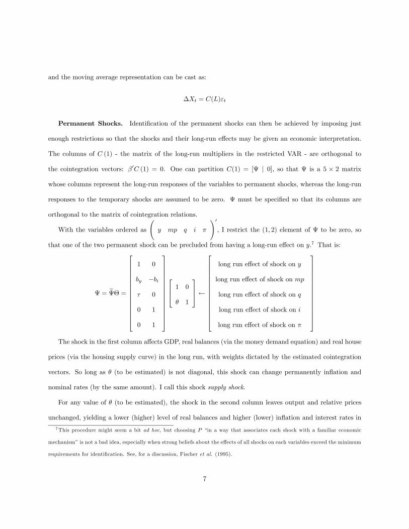
With the variables ordered as

Ãy mp q i π

!0, I restrict the (1, 2) element of Ψ to be zero, so

that one of the two permanent shock can be precluded from having a long-run effect on y.7 That is:

Ψ = eΨΘ =

1 0

by −biτ 0

0 1

0 1

1 0

θ 1

←

long run effect of shock on y

long run effect of shock on mp

long run effect of shock on q

long run effect of shock on i

long run effect of shock on π

The shock in the first column affects GDP, real balances (via the money demand equation) and real house

prices (via the housing supply curve) in the long run, with weights dictated by the estimated cointegration

vectors. So long as θ (to be estimated) is not diagonal, this shock can change permanently inflation and

nominal rates (by the same amount). I call this shock supply shock.

For any value of θ (to be estimated), the shock in the second column leaves output and relative prices

unchanged, yielding a lower (higher) level of real balances and higher (lower) inflation and interest rates in

7This procedure might seem a bit ad hoc, but choosing P “in a way that associates each shock with a familiar economic

mechanism” is not a bad idea, especially when strong beliefs about the effects of all shocks on each variables exceed the minimum

requirements for identification. See, for a discussion, Fischer et al. (1995).

7

the long run.8 One possible interpretation of this shock, following Coenen and Vega (1999), can be that of

a change in the monetary policy objective of the monetary authority: in the European experience, it can

capture a commitment to a different inflation target. I call this innovation nominal shock.

Transitory Shocks. Transitory shocks, which are assumed orthogonal to the permanent shocks and

to each other, will have no long-run effect on the variables. Following Mellander et al. (1992), they can be

identified following the recursiveness approach: the monetary policy shock has no immediate effect on output

and CPI inflation, but can contemporaneously affect real balances (by affecting liquidity supply), interest

rates and real house prices.

The demand shock has zero impact effect on CPI inflation, but potentially affects contemporaneous GDP,

by affecting its spending components, as well as house prices, real money balances, and interest rates. This

disturbance could also capture episodes originating in the housing market, such as temporary tax advantages

to housing investment or a sudden increase in demand fuelled by expectations of appreciation in house prices.

The third and last shock can contemporaneously affect all variables. I call it transitory inflation shock.,

i.e. a temporary upward shift in the aggregate supply schedule of a basic AD/AS model. This shock might

for instance proxy for an oil price or an exchange rate shock, that temporarily raise the prices of imported

goods (the impulse responses are, in most of the countries, consistent with this hypothesis).

3. Properties of the data

3.1. Sources of data

The data consist of quarterly observations on output, a monetary aggregate, consumer prices, house prices

and a nominal short-term interest rate.

French data for house prices are from the residential house price index calculated by the Banque de

France.9 German data are from the Aufina Residential Price Index: the original series was annual, and

8Opposite signs on real balances and on nominal rates only obtain if the estimated cointegrating vector between money,

output and interest rates yields coefficients of the same sign on mp and i.9This index is described in Grunspan (1998, Asset Prices Over Twenty Years, unpublished manuscript). Since 1978, an

8

a quarterly one was obtained via interpolation assuming an ARIMA(1,2,0) in the log of original series.10

Data for Italy are from the residential property price index calculated by “Il Consulente Immobilare” (with

elaboration by the Banca d’Italia); the original semi-annual frequency was converted into quarterly via

ARIMA(1,2,0) interpolation. Spanish data come from the “Residential Property Price Index per Square

Meter” calculated by the Ministerio de Economia y Hacienda. For Sweden, the data were provided by the

Central Statistical Office House Price Index.11 The UK data are from the Nationwide house price index for

all properties.

All the time series are available approximately from the mid ’70s, with the exception of Spain (where the

house prices series starts in 1987) and the UK (1963). In order to analyze similar periods, the estimation

period for the UK begins in 1973. The resulting samples are as follows: for France, 1978Q1-1997Q4; for Ger-

many, 1973Q1-1998Q3; for Italy, 1973Q1-1998Q2; for Spain, 1987Q4-1998Q4; for Sweden, 1977Q4-1998Q4;

for the UK, 1973Q1-1998Q3. House price and consumer price indices are shown in Figure 1. The Figure

provides evidence of the large swings in house prices that have occurred in the last decades, with prolonged

cycles of increasingly rising prices followed by slumps; oscillations in real house prices have been particularly

strong in Sweden and the UK; periods of falling nominal house prices have been common.

The other series were obtained from International Financial Statistics: y is the (log of) GDP at constant

prices, seasonally adjusted; i is a short-term interest rate, expressed in percentages, namely money market

rate for Italy, call money rate for France and Germany, 3 months T-Bills rate for Spain, Sweden and the

UK; real money mp is the log of M2 for France, Spain and Sweden; M1 for Germany, Italy and the UK, all

deflated by the consumer price index. In the last three countries, M1 produced more plausible estimates of

annual index of residential property prices has been estimated based on the portfolio of the FNAIM national federation of real

estate agents, which comprises 220,000 properties. The Banque de France has then transformed this index into a quarterly one

by profiling using the index of the Chambre Syndicale des notaires for old unoccupied apartments sold in Paris.10The AUFINA/ERA index shows the average price for a cubic metre enclosed area for a 3-year-old house with an average

index. It is constructed through surveys conducted by AUFINA/ERA across real estate agents in the country. In the words

of Holmans (1994), “German house price history is far from firm”. However, the series provided by Aufina is similar to that

constructed by Holmans (1994) using city-level data provided by the estate agency Ring Deutscher Makler.11The Swedish house price series is constructed as weighted mean of primary and leisure homes.

9

the cointegration vectors and of the responses to shocks. Inflation π is measured by the annualised quarterly

change of the logged CPI.

For each country, the estimated VAR contained a lag length of 3 (France, Spain, Sweden) or 4 (Germany,

Italy, UK), depending on which was sufficient to obtain noiselike residuals. Two dummies were used to

correct for German reunification (1990Q3 and 1991Q1). An impulse dummy variable for UK for 1987Q1 was

introduced to capture a coverage break in the money+quasi-money series.

3.2. Unit root and Cointegration Tests

As a preliminary step and in order to specify the model correctly, the long-run properties of the time-series

- degree of integration and the presence of cointegration relationships - must be characterised.

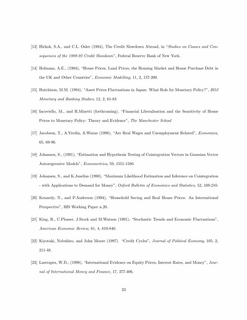
Unit root tests. Two univariate unit-root tests were conducted, the augmented Dickey-Fuller test and

the Phillips-Perron (1988) test. Tables 1 and 2 report the results from the tests. The evidence from the tests

suggests that the variables are I(1), although, according to the Phillips-Perron test, in some cases the null

hypothesis of a unit root in the inflation rate is rejected in favour of stationarity.

Cointegration tests. The cointegration vectors were estimated with the multivariate cointegration

techniques developed by Johansen and Juselius (1990). According to the λ-max statistic, the null hypothesis

of no cointegration versus one cointegration vector, of one cointegration vector versus two was rejected at the

90% confidence level in all countries. Three cointegration vectors were suggested in France, Germany and

Sweden, whereas two appear more likely in Germany and Italy, and four in Spain. On plausibility grounds,

and in order to have more easily comparable results across countries, a common rank of 3 was chosen.

3.3. Cointegration relations

Table 3 reports the estimated (restricted) cointegration vectors for each country, together with p-values for

the over-identifying restrictions. The restrictions were rejected at the 95% confidence level in Sweden and

10

Spain.12 Since it has been shown (Jacobson et al., 1998) that the likelihood ratio test for hypothesis about

the cointegration vectors for a given rank tends to be oversized, I prefer to present for reasons of space only

the restricted vectors, with standard errors in parentheses: the loss of information should not be great, as

unrestricted and restricted vectors (upon a convenient rotation of the latter) should be similar. I find that:

• The income elasticity of money demand by is greater than one whenever it is not restricted to unity.

This could be the consequence of omitting wealth variables in the money demand, such as housing

wealth, which is positively correlated with income.

• The semi-elasticity of money demand with respect to the short-term interest rate, bi, is negatively

signed in two cases out of six. For France and Sweden, the implied elasticity of realM2 is positive: yet

a positive elasticity is plausible on theoretical grounds, as a negative coefficient should be expected a

priori only on a narrow money measure.

• The cointegration vector between real house prices and GDP favours an interpretation of the long-run

upward trend in house prices that, despite the short length of the series, is consistent across countries.13

The point estimates of the coefficient τ range from a lower limit of .063 for Germany to 1.69 for Spain.

Although fully consistent with economic theory, these estimates should be treated with care, as they

are sensitive to the period they cover: cointegration between real house prices and output can be a

statistical property of the data, but putting structural emphasis on cross-country differences would be

probably too ambitious.

12 In France and Sweden, I imposed unit elasticity of money with respect to income, as the unrestricted income elasticity was

measured with great imprecision and led to implausible estimates for the money demand elasticities.13This is broadly in line with the cross-country evidence in the paper by Kennedy and Anderson (1994).In 13 out of 15 nations

real house prices were higher in 1993 than in 1970. Cutler (1995) shows similar evidence for the G7 economies from 1970 to

1992.

11

4. Empirical evidence

4.1. Impulse Responses

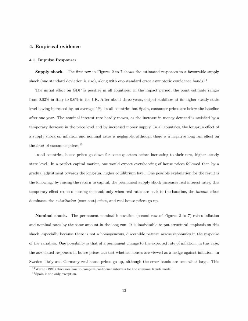
Supply shock. The first row in Figures 2 to 7 shows the estimated responses to a favourable supply

shock (one standard deviation is size), along with one-standard error asymptotic confidence bands.14

The initial effect on GDP is positive in all countries: in the impact period, the point estimate ranges

from 0.02% in Italy to 0.6% in the UK. After about three years, output stabilises at its higher steady state

level having increased by, on average, 1%. In all countries but Spain, consumer prices are below the baseline

after one year. The nominal interest rate hardly moves, as the increase in money demand is satisfied by a

temporary decrease in the price level and by increased money supply. In all countries, the long-run effect of

a supply shock on inflation and nominal rates is negligible, although there is a negative long run effect on

the level of consumer prices.15

In all countries, house prices go down for some quarters before increasing to their new, higher steady

state level. In a perfect capital market, one would expect overshooting of house prices followed then by a

gradual adjustment towards the long-run, higher equilibrium level. One possible explanation for the result is

the following: by raising the return to capital, the permanent supply shock increases real interest rates; this

temporary effect reduces housing demand; only when real rates are back to the baseline, the income effect

dominates the substitution (user cost) effect, and real house prices go up.

Nominal shock. The permanent nominal innovation (second row of Figures 2 to 7) raises inflation

and nominal rates by the same amount in the long run. It is inadvisable to put structural emphasis on this

shock, especially because there is not a homogeneous, discernible pattern across economies in the response

of the variables. One possibility is that of a permanent change to the expected rate of inflation: in this case,

the associated responses in house prices can test whether houses are viewed as a hedge against inflation. In

Sweden, Italy and Germany real house prices go up, although the error bands are somewhat large. This

14Warne (1993) discusses how to compute confidence intervals for the common trends model.15 Spain is the only exception.

12

increase in expected inflation elicits an upward response of nominal interest rates, which is suggestive of an

anti-inflationary monetary policy from the monetary authority.

Monetary shock. The third row of Figures 2 to 7 shows that the monetary shock elicits upward

pressure in interest rate, a contraction in the monetary aggregate,16 and a temporary decline in output,

which bottoms out approximately between 4 and 9 quarters after the impulse. These are general indications

of a contractionary monetary policy stance.

Consumer prices remain above the baseline for one year in the UK, Germany and Sweden. In the UK and

Sweden this pattern is plausible, as variable rate mortgage costs have a large weight in household budgets,

as well as on measured inflation; in Germany, the initial CPI rise might occur if the monetary shock captures

some systematic response to unaccounted disturbances generating inflationary pressures. Unlike consumer

prices, house prices respond more strongly, and, with some differences across countries, they significantly

decrease. I defer a more detailed discussion of these issues to the next section.

Demand shock. The demand shock results in short-term output effects with consumer prices fixed in

the impact period. Following Gerlach and Smets (1995), it is possible to label this disturbance “demand

shock” since it elicits positive output and price responses and due to its transitory imprint on the real

variables in the system. The responses (row 4 of Figures 2 to 7) show an increase in real house prices

that peaks after about 2 years and dies out only after 5/6 years. This is consistent with the idea that the

shock might be a combination of various factors, such as: temporary tax incentives that give an advantage

to invest in housing; increase in housing demand stemming from optimistic expectations; an increase in

aggregate demand deriving from other sources (e.g. devaluation of national currency under fixed exchange

rates) that feeds back into house price inflation with some lag.

In all countries, nominal and real interest rates go up. Output rises protractedly. Inflation goes up as

well, except in Germany. Real house price increases are particularly strong in the UK and Sweden. The

increase, whose timing closely matches that of output, lasts several years.

16Although real balances temporarily rise in France and the UK, the effect on nominal balances is unambiguously negative.

13

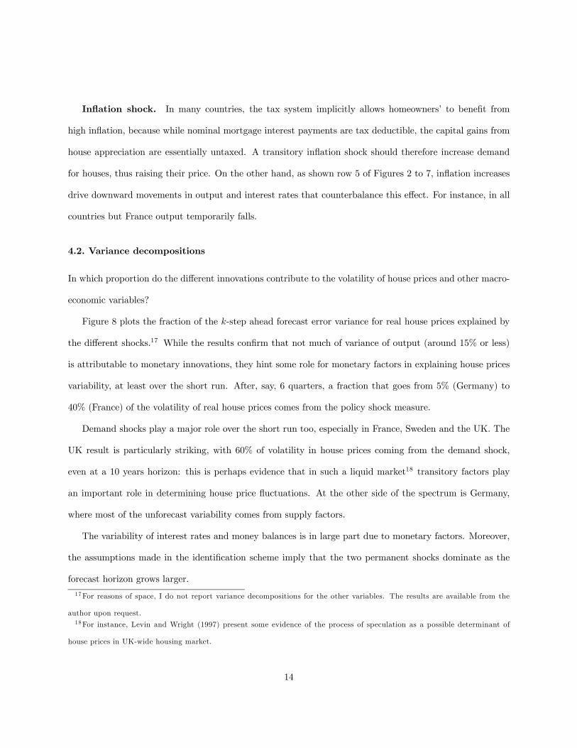
Inflation shock. In many countries, the tax system implicitly allows homeowners’ to benefit from

high inflation, because while nominal mortgage interest payments are tax deductible, the capital gains from

house appreciation are essentially untaxed. A transitory inflation shock should therefore increase demand

for houses, thus raising their price. On the other hand, as shown row 5 of Figures 2 to 7, inflation increases

drive downward movements in output and interest rates that counterbalance this effect. For instance, in all

countries but France output temporarily falls.

4.2. Variance decompositions

In which proportion do the different innovations contribute to the volatility of house prices and other macro-

economic variables?

Figure 8 plots the fraction of the k-step ahead forecast error variance for real house prices explained by

the different shocks.17 While the results confirm that not much of variance of output (around 15% or less)

is attributable to monetary innovations, they hint some role for monetary factors in explaining house prices

variability, at least over the short run. After, say, 6 quarters, a fraction that goes from 5% (Germany) to

40% (France) of the volatility of real house prices comes from the policy shock measure.

Demand shocks play a major role over the short run too, especially in France, Sweden and the UK. The

UK result is particularly striking, with 60% of volatility in house prices coming from the demand shock,

even at a 10 years horizon: this is perhaps evidence that in such a liquid market18 transitory factors play

an important role in determining house price fluctuations. At the other side of the spectrum is Germany,

where most of the unforecast variability comes from supply factors.

The variability of interest rates and money balances is in large part due to monetary factors. Moreover,

the assumptions made in the identification scheme imply that the two permanent shocks dominate as the

forecast horizon grows larger.

17For reasons of space, I do not report variance decompositions for the other variables. The results are available from the

author upon request.18For instance, Levin and Wright (1997) present some evidence of the process of speculation as a possible determinant of

house prices in UK-wide housing market.

14

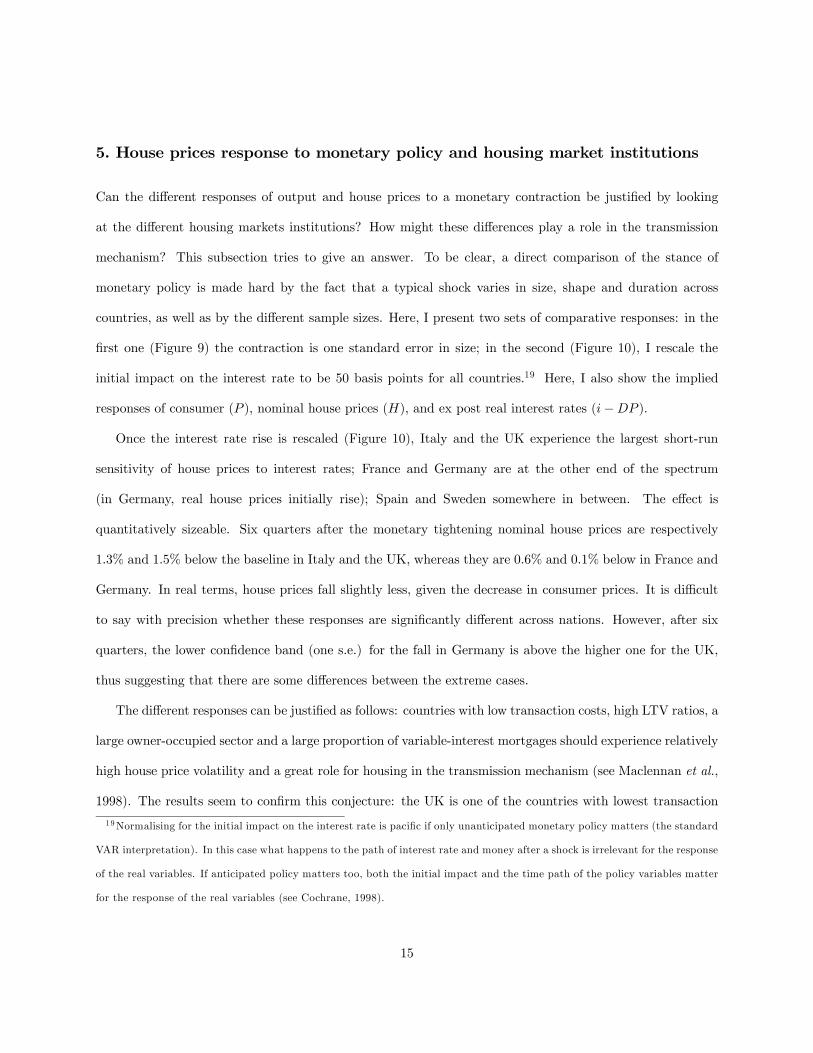
5. House prices response to monetary policy and housing market institutions

Can the different responses of output and house prices to a monetary contraction be justified by looking

at the different housing markets institutions? How might these differences play a role in the transmission

mechanism? This subsection tries to give an answer. To be clear, a direct comparison of the stance of

monetary policy is made hard by the fact that a typical shock varies in size, shape and duration across

countries, as well as by the different sample sizes. Here, I present two sets of comparative responses: in the

first one (Figure 9) the contraction is one standard error in size; in the second (Figure 10), I rescale the

initial impact on the interest rate to be 50 basis points for all countries.19 Here, I also show the implied

responses of consumer (P ), nominal house prices (H), and ex post real interest rates (i−DP ).

Once the interest rate rise is rescaled (Figure 10), Italy and the UK experience the largest short-run

sensitivity of house prices to interest rates; France and Germany are at the other end of the spectrum

(in Germany, real house prices initially rise); Spain and Sweden somewhere in between. The effect is

quantitatively sizeable. Six quarters after the monetary tightening nominal house prices are respectively

1.3% and 1.5% below the baseline in Italy and the UK, whereas they are 0.6% and 0.1% below in France and

Germany. In real terms, house prices fall slightly less, given the decrease in consumer prices. It is difficult

to say with precision whether these responses are significantly different across nations. However, after six

quarters, the lower confidence band (one s.e.) for the fall in Germany is above the higher one for the UK,

thus suggesting that there are some differences between the extreme cases.

The different responses can be justified as follows: countries with low transaction costs, high LTV ratios, a

large owner-occupied sector and a large proportion of variable-interest mortgages should experience relatively

high house price volatility and a great role for housing in the transmission mechanism (see Maclennan et al.,

1998). The results seem to confirm this conjecture: the UK is one of the countries with lowest transaction

19Normalising for the initial impact on the interest rate is pacific if only unanticipated monetary policy matters (the standard

VAR interpretation). In this case what happens to the path of interest rate and money after a shock is irrelevant for the response

of the real variables. If anticipated policy matters too, both the initial impact and the time path of the policy variables matter

for the response of the real variables (see Cochrane, 1998).

15

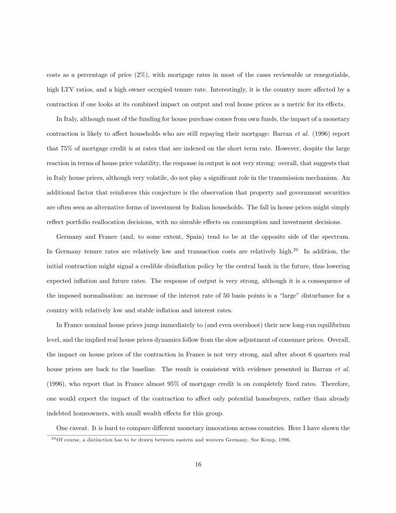
costs as a percentage of price (2%), with mortgage rates in most of the cases reviewable or renegotiable,

high LTV ratios, and a high owner occupied tenure rate. Interestingly, it is the country more affected by a

contraction if one looks at its combined impact on output and real house prices as a metric for its effects.

In Italy, although most of the funding for house purchase comes from own funds, the impact of a monetary

contraction is likely to affect households who are still repaying their mortgage: Barran et al. (1996) report

that 75% of mortgage credit is at rates that are indexed on the short term rate. However, despite the large

reaction in terms of house price volatility, the response in output is not very strong: overall, that suggests that

in Italy house prices, although very volatile, do not play a significant role in the transmission mechanism. An

additional factor that reinforces this conjecture is the observation that property and government securities

are often seen as alternative forms of investment by Italian households. The fall in house prices might simply

reflect portfolio reallocation decisions, with no sizeable effects on consumption and investment decisions.

Germany and France (and, to some extent, Spain) tend to be at the opposite side of the spectrum.

In Germany tenure rates are relatively low and transaction costs are relatively high.20 In addition, the

initial contraction might signal a credible disinflation policy by the central bank in the future, thus lowering

expected inflation and future rates. The response of output is very strong, although it is a consequence of

the imposed normalisation: an increase of the interest rate of 50 basis points is a “large” disturbance for a

country with relatively low and stable inflation and interest rates.

In France nominal house prices jump immediately to (and even overshoot) their new long-run equilibrium

level, and the implied real house prices dynamics follow from the slow adjustment of consumer prices. Overall,

the impact on house prices of the contraction in France is not very strong, and after about 6 quarters real

house prices are back to the baseline. The result is consistent with evidence presented in Barran et al.

(1996), who report that in France almost 95% of mortgage credit is on completely fixed rates. Therefore,

one would expect the impact of the contraction to affect only potential homebuyers, rather than already

indebted homeowners, with small wealth effects for this group.

One caveat. It is hard to compare different monetary innovations across countries. Here I have shown the

20Of course, a distinction has to be drawn between eastern and western Germany. See Kemp, 1996.

16

responses with and without normalisation of the initial impact on the nominal rate. The normalization has

the virtue of providing a useful benchmark now that four of these countries are under a common monetary

policy; the second procedure compares in all the countries a “typical” benchmark shock over the period in

question. Despite these difficulties, the overall evidence suggests a link between housing market institutions

on the one hand and sensitivity of house prices to a monetary disturbance on the other. Although it deserves

future research, comparing output responses is perhaps harder, especially because it is problematic to control

for other factors that influence the transmission mechanism.

6. An informal interpretation of house price movements

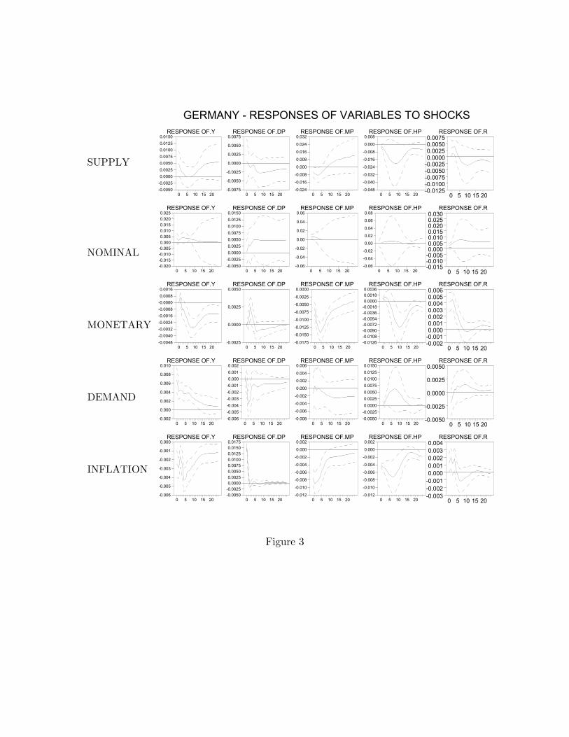
Figures 11 to 16 plot for each country real house prices, inflation, interest rates and GDP in the first row, and

estimates of the five structural shocks in the second.21 For ease of interpretation, I construct nine quarter,

centered moving averages for each of the otherwise uncorrelated disturbances. I focus only on some specific,

relevant periods of significant house prices changes for each country. The overall picture that emerges is that

no boom can be easily associated with a single source of macroeconomic fluctuations. Each major variation

in house prices appears to have been driven by a combination of factors pushing in the same direction.

FRANCE. France had a boom during the year 1980, with house prices peaking at the beginning of

the 1981 and falling by 15% in real terms in the following two years; a similar boom-bust occurred from 1985

to 1989 (prices peaked at the end of 1987). After a peak at the beginning of 1991, prices had fallen in real

terms by about 25% at the beginning of year 1997. Demand shocks seem to have played an important role

in driving house price fluctuations, together with other transitory factors. The 1985 - 1987 boom followed

a period of positive supply shocks and expansionary monetary policy. Money and credit growth were rising

(thanks to abolition of credit control measures known as “encadrement du credit”: see Hickok and Osler,

1994). Instead, the growth of prices from 1989 to 1991 seems the effect of demand shocks: monetary policy

appears to have been tight over that period, and might have contributed to the fall in house prices that

21The historical decomposition of the time series yield similar results. They are available from the author upon request.

17

started at the beginning of 1991. Between 1997 and 1998, house prices showed a slow recovery. Various fiscal

incentives and new contracts offered to potential house buyers (such as the introduction of the “propriétée

allégée”) managed to stimulate the demand again.

GERMANY. The German house price boom of the late ’80s - with the real house price index up 15%

in the 4 years from 1986 to 1990, but much larger increases in the big cities - seems due to a positive demand

shock. The “demand” shock has its roots not just in the booming economy of the late ’80s, but also in

specific housing market episodes: in 1987 capital gains tax exemptions were introduced; from 1991, it was

possible to deduct interest payments up to DM 12,000 per annum for the first three years from the purchase

of a newly built house. In addition, the big cities saw an influx of migrants from the east of Germany as well

as from elsewhere which placed pressure on the west German housing market and helped to create a new

housing shortage there.22

ITALY. The main increases in house prices occurred between 1979 and 1981 and in the late ’80s. A

sharp drop between 1982 and 1985, with prices falling by one third in real terms, followed the first boom.

After the late ’80s rise, prices fell 15% in real terms between 1993 and 1996. Figure 13 highlights that nominal

factors and demand shocks played a distinctive role in driving house prices down from 1993 onwards. Among

the negative demand shocks, a role could have been played by policies that revised upward the fiscal value

(“valore catastale”) of the residential property. This made investment in housing unattractive in a period

of economic recession, low household expectations about future incomes, and near saturation of the market,

with tenure rates as high as 78%, one of the highest levels in Europe (Censis, 1996). The inversion in the

falling trend at the end of the sample reflects the effect of falling real interest rates. In the Italian case, this

episode probably implies not only cheaper mortgages but also reduction in yields from government securities,

which have always represented a traditional alternative investment to property.

22See Kemp, 1996, Housing Policy in the EU Member States, unpublished manuscript.

18

SPAIN. Positive demand and supply shocks seem to have driven the late ’80s boom. Only a small

fraction of the fluctuations in house prices seems attributable to the monetary policy stance, which was

neutral during that period. The decline in real house prices for most of the ’90s started with the recession

in 1992 and 1993 and was driven by tighter monetary policy and negative demand shocks. The increase in

the late ’90s is the result of the prolonged decrease in real interest rates as well as the economic expansion,

alongside the increased demand for second homes from people in need to get rid of black money in the run-up

to the single currency.

SWEDEN. Demand and monetary policy shocks drove the housing boom of the late ’80s: house prices

went up 35% in real terms between 1986 and 1989, and fell by almost the same amount in the years from

1991 to 1993. Loose fiscal policy, deregulation of the financial markets (ceilings on bank lending rates and

quantitative controls on bank loans were abolished in 1985) and a tax system that encouraged debt-financed

consumption spurred aggregate demand and increased asset prices. Demand shocks were consistently positive

in all years until 1990, when a quickly deepening recession set in. An international recession, a reformed

tax system that abolished investment allowances and falling asset prices contributed to the severity of the

downturn (see Berg and Gröttheim, 1997).

UK. Between 1974 and 1998, the UK has experienced two main house price boom-busts cycles, the

first from 1978 to 1982, the second from 1983 to 1992. During the first (smaller) cycle, house prices rose in

real terms by 20%, hit a peak at the end of 1979, and then fell by 15%. In the second (bigger) cycle, real

house prices rose about 60%, peaked in 1989, and then fell by 47%, bottoming at the end of 1995.

The house price boom of the late ’80s could have been driven by a combination of three factors: positive

supply and demand shocks and expansionary monetary policy. Among the factors that contributed:

1) demand side factors: the announcement in 1988 that mortgage tax relief would be restricted to £30,000

per residence regardless of the number of borrowers boosted housing demand. Financial liberalization permit-

ted higher gearing, as borrowers were able to obtain higher LTV ratios. In addition, optimistic expectations

about rising incomes played a role: the experience of housing appreciation reinforced expectations of further

19

appreciation to come.

2) monetary policy: a loose monetary policy followed the appreciation of the pound from 1987.

3) supply side factors: the (permanent) income rise led to a rise in housing demand, but supply grew

more slowly, with construction of social housing falling to a small fraction of its level in the 1970s.23

The early 1990s bust derived from the reversal of most of these factors. Interest rates rose. Income growth

expectations weakened. The introduction of a new tax on houses (the Council Tax) depressed property values

further. Mortgage lenders tightened their lending criteria, in a reversal of the financial liberalization of the

late ’80s. The increase of the late ’90s (from 1996) seems to reflect more demand and supply shocks than

loose monetary policy conditions. Besides the traditional factors outlined above, a “demand shock” has been

represented, particularly in the London area, by the ‘buy-to-let’ boom, supported by a change in the attitude

of mortgage lenders towards landlords.

7. Conclusions

This paper has shown that the dynamics of house prices can be dealt with using a tractable VAR framework

in a straightforward way. I have developed and estimated a simple macroeconometric model driven by five

exogenous disturbances, all of which can have effects on house price inflation. In particular, I have shown

that monetary policy shocks can have serious effects on house prices. What supports these findings is that

a set of reasonable identifying assumptions yields plausible results for the responses of money, consumer

prices and output to shocks. To this, I add a relatively new piece of evidence, showing that, unlike consumer

prices, house price inflation is highly sensitive to the forces driving economic fluctuations. Although this

result is not surprising in itself - after all, house prices, as asset prices, can be expected to reflect shifts

23 It is often argued that financial liberalisation could have contributed to the housing boom in the ’80s: restrictions on bank

lending were abolished in 1980, enabling banks to compete with building societies; average LTV ratios for first time buyers

rose from .74 in 1980 to .86 in the mid 80s. Yet the boom came several years after the deregulation, suggesting that financial

liberalisation itself cannot be the sole cause. Demographic factors are mentioned too (population in the 20-29 age range rose

by 1.3 million over the 80s, compared to .1 million over the previous decade) but they can be hardly considered shocks: such a

phenomenon was predictable and one would expect the main impact of demographics to be on quantities rather than prices.

20

in expectations more quickly than consumer prices -, it is encouraging that it has been obtained with a

highly stylised macroeconomic model, which in other respects closely matches the predictions of a standard

IS-LM-Phillips curve paradigm.

The results hint that different housing and credit market institutions play a role in this transmission

mechanism: however, as institutions change, this relationship might change too. Fiscal, regulatory and legal

structure and the new monetary policy regime are likely to affect this relationship.24

The debate on asset prices and the business cycle has a long tradition in macroeconomics, at least since

Irving Fisher (1911) argued that policymakers should aim to stabilise a broad price index including, besides

goods and services, shares, bonds and property. There are widespread concerns on whether expansionary

monetary policies are at the origin of dramatic asset price changes. With respect to the housing market,

the evidence presented here suggests that the unsystematic component of monetary policy (and other macro

factors) can play an important role in driving asset price fluctuations.

24A maintained assumption here is that the link between house prices and the macroeconomy has remained relatively stable

over time. Of course, the period analysed has witnessed several changes in the housing market and in the financial system.

Iacoviello and Minetti (forthcoming) explore the issue analysing the impact of financial liberalisation on the link between

monetary policy and house prices. They use vector autoregressions to study the role of monetary policy shocks in house price

fluctuations in Finland, Sweden and the UK, characterised by financial liberalisation episodes over the last twenty years. They

find that the response of house prices to interest rate surprises is bigger and more persistent in periods characterised by more

liberalised financial markets.

21

References

[1] Barran, F., V. Coudert and B. Mojon (1996), “The Transmission of the Monetary Policy in the

European Countries”, London School of Economics, Financial Markets Group, Special Paper, No.86.

[2] Berg, C., and R. Gröttheim (1997), “Monetary Policy in Sweden since 1992”, BIS Public Policy paper

no.2.

[3] Bernanke, B.S., and M. Gertler (1999), “Monetary Policy and Asset Price Volatility”, Federal Reserve

Bank of Kansas City Economic Review, 4, 5-12.

[4] Censis (1996), Trentesimo Rapporto sulla Situazione Sociale del Paese, FrancoAngeli, Milano.

[5] Cochrane, J. (1998), “What do the VARs Mean? Measuring the Output Effects of Monetary Policy”,

Journal of Monetary Economics, 41, 2, 277-300.

[6] Coenen, G., and J.L. Vega (1999), “The Demand for M3 in the Euro Area”, ECB Working Paper no.6

[7] Cutler, J. (1995), “The Housing Market and the Economy”, Bank of England Quarterly Bulletin, 35,

3, 260-269.

[8] Ericsson, N.R. (1998), “Empirical Modelling of Money Demand”, Empirical Economics, 23, 3, 295-315.

[9] Fisher, I. (1911), The Purchasing Power of Money, The MacMillan Press.

[10] Fischer, L., P.Fackler and D.Orden (1995), “Long-Run Identifying Restrictions for an Error-correction

Model of New Zeland Money, Prices and Output”, Journal of International Money and Finance, 14,

127-147.

[11] Gali, J. (1992), “How Does the IS-LMModel Fit Postwar U.S. Data?”, Quarterly Journal of Economics,

107, 2, 709-738.

[12] Gerlach, S., and F.Smets (1995), “The Monetary Transmission Mechanism: Evidence from the G7

Countries”, CEPR Discussion Paper No. 1219.

22

[13] Hickok, S.A., and C.L. Osler (1994), The Credit Slowdown Abroad, in “Studies on Causes and Con-

sequences of the 1989-92 Credit Slowdown”, Federal Reserve Bank of New York.

[14] Holmans, A.E., (1994), “House Prices, Land Prices, the Housing Market and House Purchase Debt in

the UK and Other Countries”, Economic Modelling, 11, 2, 157-200.

[15] Hutchison, M.M. (1994), “Asset Prices Fluctuations in Japan: What Role for Monetary Policy?”, BOJ

Monetary and Banking Studies, 12, 2, 61-83

[16] Iacoviello, M., and R.Minetti (forthcoming), “Financial Liberalisation and the Sensitivity of House

Prices to Monetary Policy: Theory and Evidence”, The Manchester School

[17] Jacobson, T., A.Vredin, A.Warne (1998), “Are Real Wages and Unemployment Related”, Economica,

65, 69-96.

[18] Johansen, S., (1991), “Estimation and Hypothesis Testing of Cointegration Vectors in Gaussian Vector

Autoregressive Models”, Econometrica, 59, 1551-1580.

[19] Johansen, S., and K.Juselius (1990), “Maximum Likelihood Estimation and Inference on Cointegration

- with Applications to Demand for Money”, Oxford Bulletin of Economics and Statistics, 52, 169-210.

[20] Kennedy, N., and P.Anderson (1994), “Household Saving and Real House Prices: An International

Perspective”, BIS Working Paper n.20.

[21] King, R., C.Plosser, J.Stock and M.Watson (1991), “Stochastic Trends and Economic Fluctuations”,

American Economic Review, 81, 4, 819-840.

[22] Kiyotaki, Nobuhiro, and John Moore (1997). “Credit Cycles”, Journal of Political Economy, 105, 2,

211-48.

[23] Lastrapes, W.D., (1998), “International Evidence on Equity Prices, Interest Rates, and Money”, Jour-

nal of International Money and Finance, 17, 377-406.

23

[24] Levin, E.J., and R.E.Wright (1997), “The Impact of Speculation on House Prices in the United King-

dom”, Economic Modelling, 14, 567-589.

[25] MacKinnon, J.G. (1991), “Critical Values for Cointegration Tests”, in R.Engle and C.Granger eds.,

Long-Run Economic Relationships, Oxford University Press, Oxford.

[26] Maclennan, D., J.Muellbauer, and M.Stephens (1998), “Asymmetries in Housing and Financial Market

Institutions and EMU”, Oxford Review of Economic Policy, 14, 3, 54-80.

[27] Mellander, E., A.Vredin and A.Warne (1992), “Stochastic Trends and Economic Fluctuations in a

Small Open Economy”, Journal of Applied Econometrics, 7, 369-394.

[28] Miles, D. (1995), Housing, financial markets and the wider economy, John Wiley and Sons, New York.

[29] Phillips, P.C.B., and P.Perron (1988), “Testing for a Unit Root in Time Series Regression”, Biometrika,

75, 335-346.

[30] Poterba, J. (1984), “Tax Subsidies to Owner-Occupied Housing: An Asset Market Approach”, Quar-

terly Journal of Economics, 99, 729-752.

[31] Poterba, J. (1991), “House Price Dynamics: The Role of Tax Policy and Demography”, Brookings

Papers on Economic Activity, 2, 143-203.

[32] Shigemi, Y., (1995), “Asset Inflation in Selected Countries”, BOJ Monetary and Banking Studies, 13,

2, 1995.

[33] Warne, A. (1993), “A Common Trends Model: Identification, Estimation and Inference”, seminar

paper No.555, IIES, Stockholm.

24

Tables

Table 1: Augmented Dickey-Fuller unit root tests

FRANCE GERMANY ITALY SPAIN SWEDEN U.K.

y -0.10 0.14 -2.23 -0.99 -0.62 -0.09

mp -1.27 1.10 -0.88 -0.21 -2.07 -0.14

q -2.61 -2.36 -2.31 -2.64 -2.39 -1.40

i -0.97 -2.62 -1.59 -0.21 -1.67 -2.31

π -0.65 -2.20 -1.61 -0.68 -1.77 -2.76

ADF unit root tests statistics for the series, with a lag length of 3 for France, Spain and Sweden, 4 for

Germany, Italy and the UK; * indicates rejection of the null hypothesis of unit root at the 95% confidence

level, ** at the 99% level - depending on the sample size, the 95% MacKinnon (1991) critical value ranges

from -2.89 to -2.92 -.

25

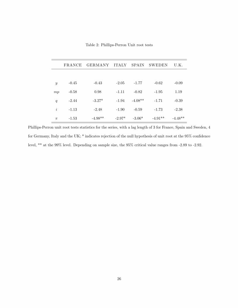
Table 2: Phillips-Perron Unit root tests

FRANCE GERMANY ITALY SPAIN SWEDEN U.K.

y -0.45 -0.43 -2.05 -1.77 -0.62 -0.09

mp -0.58 0.98 -1.11 -0.82 -1.95 1.19

q -2.44 -3.27* -1.94 -4.08** -1.71 -0.39

i -1.13 -2.48 -1.90 -0.59 -1.73 -2.38

π -1.53 -4.98** -2.97* -3.06* -4.91** -4.48**

Phillips-Perron unit root tests statistics for the series, with a lag length of 3 for France, Spain and Sweden, 4

for Germany, Italy and the UK; * indicates rejection of the null hypothesis of unit root at the 95% confidence

level, ** at the 99% level. Depending on sample size, the 95% critical value ranges from -2.89 to -2.92.

26

Table 3: Parameter estimates of the cointegration vectors

Country Period CV1 CV2 CV3 P-value #cv 90%(λ-max)

France 78:4 - 97:4 mp2 = y + 5.044(1.074)

i q = .373(.05)

y i = π .11 3

Germany 73:1 - 98:3 mp1 = 2.075(.029)

y + .35(.272)

i q = .063(.102)

y i = π .10 2

Italy 73:1 - 98:2 mp1 = 1.495y + 3.01(.409)

i q = 1.24(.187)

y i = π .53 2

Spain 87:4 - 98:4 mp2 = 1.65(.18)

y − 3.67(.12)

i q = 1.69(.21)

y i = π .01 3

Sweden 77:4 - 98:4 mp2 = y + 5.37(.834)

i q = .864(.159)

y i = π .04 3

UK 73:1 - 98:3 mp1 = 1.926(.12)

y − 7.02(.515)

i q = .63(.11)

y i = π .82 4

Parameter estimates of the three cointegration vectors (standard errors in brackets). The sixth column shows

the p-value of the likelihood ratio test statistic for overidentifying restrictions on the cointegration vectors.

The last column refers to the number of cointegration vectors suggested by the λ-max statistic at the 90%

confidence level.

27

Figures for “House Prices and Business Cycles in Europe: A VAR

Analysis”

Figure 1

HOUSE PRICES AND CONSUMER PRICESIndex: 1990 = 100

FRANCE

1973 1976 1979 1982 1985 1988 1991 1994 199725

50

75

100

125HOUSE PRICESCONSUMER PRICES

GERMANY

1973 1976 1979 1982 1985 1988 1991 1994 199750

75

100

125HOUSE PRICESCONSUMER PRICES

ITALY

1973 1976 1979 1982 1985 1988 1991 1994 19970

20

40

60

80

100

120

140

160HOUSE PRICESCONSUMER PRICES

SPAIN

1973 1976 1979 1982 1985 1988 1991 1994 19970

25

50

75

100

125

150HOUSE PRICESCONSUMER PRICES

SWEDEN

1973 1976 1979 1982 1985 1988 1991 1994 199720

40

60

80

100

120

140HOUSE PRICESCONSUMER PRICES

UNITED KINGDOM

1973 1976 1979 1982 1985 1988 1991 1994 19970

20

40

60

80

100

120

140HOUSE PRICESCONSUMER PRICES

SUPPLY

NOMINAL

MONETARY

DEMAND

INFLATION

Figure 2

FRANCE - RESPONSES OF VARIABLES TO SHOCKSRESPONSE OF. Y

0 5 10 15 200.0000

0.0025

0.0050

0.0075

0.0100

0.0125

0.0150

0.0175

RESPONSE OF. Y

0 5 10 15 20-0.015

-0.010

-0.005

0.000

0.005

0.010

0.015

RESPONSE OF. Y

0 5 10 15 20-0.0042-0.0036-0.0030-0.0024-0.0018-0.0012-0.0006-0.00000.00060.0012

RESPONSE OF. Y

0 5 10 15 20-0.002-0.0010.0000.0010.0020.0030.0040.0050.006

RESPONSE OF. Y

0 5 10 15 20-0.002

-0.001

0.000

0.001

0.002

0.003

0.004

0.005

RESPONSE OF. DP

0 5 10 15 20-0.0150-0.0125-0.0100-0.0075-0.0050-0.00250.00000.00250.0050

RESPONSE OF. DP

0 5 10 15 20-0.004

-0.002

0.000

0.002

0.004

0.006

0.008

0.010

RESPONSE OF. DP

0 5 10 15 20-0.0075

-0.0050

-0.0025

0.0000

0.0025

0.0050

0.0075

RESPONSE OF. DP

0 5 10 15 20-0.002-0.0010.0000.0010.0020.0030.0040.0050.0060.007

RESPONSE OF. DP

0 5 10 15 20-0.002

0.000

0.002

0.004

0.006

0.008

0.010

0.012

RESPONSE OF. MP

0 5 10 15 20-0.005

0.000

0.005

0.010

0.015

0.020

0.025

0.030

RESPONSE OF. MP

0 5 10 15 20-0.01

0.00

0.01

0.02

0.03

0.04

RESPONSE OF. MP

0 5 10 15 20-0.004

-0.002

0.000

0.002

0.004

0.006

0.008

0.010

RESPONSE OF. MP

0 5 10 15 20-0.0075

-0.0050

-0.0025

0.0000

0.0025

0.0050

RESPONSE OF. MP

0 5 10 15 20-0.006-0.005-0.004-0.003-0.002-0.0010.000

0.0010.002

RESPONSE OF. HP

0 5 10 15 20-0.025-0.020

-0.015-0.010

-0.0050.000

0.0050.0100.015

RESPONSE OF. HP

0 5 10 15 20-0.032

-0.024

-0.016

-0.008

0.000

0.008

0.016

RESPONSE OF. HP

0 5 10 15 20-0.030-0.025-0.020-0.015-0.010-0.0050.0000.0050.0100.015

RESPONSE OF. HP

0 5 10 15 20-0.010-0.0050.0000.0050.0100.0150.020

0.0250.030

RESPONSE OF. HP

0 5 10 15 20-0.0075-0.0050-0.00250.00000.00250.00500.00750.01000.01250.0150

RESPONSE OF. R

0 5 10 15 20-0.0096-0.0080

-0.0064-0.0048

-0.0032-0.0016

-0.00000.00160.0032

RESPONSE OF. R

0 5 10 15 20-0.008-0.006

-0.004-0.002

0.0000.002

0.0040.0060.008

RESPONSE OF. R

0 5 10 15 20-0.0030

0.0000

0.0030

0.0060

0.0090

RESPONSE OF. R

0 5 10 15 20-0.0100-0.0075-0.0050-0.00250.00000.00250.0050

0.00750.0100

RESPONSE OF. R

0 5 10 15 20-0.0016-0.00080.00000.00080.00160.00240.00320.00400.00480.0056

SUPPLY

NOMINAL

MONETARY

DEMAND

INFLATION

Figure 3

GERMANY - RESPONSES OF VARIABLES TO SHOCKSRESPONSE OF.Y

0 5 10 15 20-0.0050-0.00250.00000.00250.00500.00750.01000.01250.0150

RESPONSE OF.Y

0 5 10 15 20-0.020-0.015-0.010-0.0050.0000.0050.0100.0150.0200.025

RESPONSE OF.Y

0 5 10 15 20-0.0048-0.0040-0.0032-0.0024-0.0016-0.0008-0.00000.00080.0016

RESPONSE OF.Y

0 5 10 15 20-0.002

0.000

0.002

0.004

0.006

0.008

0.010

RESPONSE OF.Y

0 5 10 15 20-0.006

-0.005

-0.004

-0.003

-0.002

-0.001

0.000

RESPONSE OF.DP

0 5 10 15 20-0.0075

-0.0050

-0.0025

0.0000

0.0025

0.0050

0.0075

RESPONSE OF.DP

0 5 10 15 20-0.0050-0.00250.00000.00250.00500.00750.01000.01250.0150

RESPONSE OF.DP

0 5 10 15 20-0.0025

0.0000

0.0025

0.0050

RESPONSE OF.DP

0 5 10 15 20-0.006-0.005-0.004-0.003-0.002-0.0010.0000.0010.002

RESPONSE OF.DP

0 5 10 15 20-0.0050-0.00250.00000.00250.00500.00750.01000.01250.01500.0175

RESPONSE OF.MP

0 5 10 15 20-0.024

-0.016

-0.008

0.000

0.008

0.016

0.024

0.032

RESPONSE OF.MP

0 5 10 15 20-0.06

-0.04

-0.02

0.00

0.02

0.04

0.06

RESPONSE OF.MP

0 5 10 15 20-0.0175

-0.0150

-0.0125

-0.0100

-0.0075

-0.0050

-0.0025

0.0000

RESPONSE OF.MP

0 5 10 15 20-0.008

-0.006

-0.004

-0.002

0.000

0.002

0.004

0.006

RESPONSE OF.MP

0 5 10 15 20-0.012

-0.010

-0.008

-0.006

-0.004

-0.002

0.000

0.002

RESPONSE OF.HP

0 5 10 15 20-0.048

-0.040

-0.032

-0.024

-0.016

-0.008

0.000

0.008

RESPONSE OF.HP

0 5 10 15 20-0.06

-0.04

-0.02

0.00

0.02

0.04

0.06

0.08

RESPONSE OF.HP

0 5 10 15 20-0.0126-0.0108-0.0090-0.0072-0.0054-0.0036-0.00180.00000.00180.0036

RESPONSE OF.HP

0 5 10 15 20-0.0050-0.00250.00000.00250.00500.00750.01000.01250.0150

RESPONSE OF.HP

0 5 10 15 20-0.012

-0.010

-0.008

-0.006

-0.004

-0.002

0.000

0.002

RESPONSE OF.R

0 5 10 15 20-0.0125-0.0100-0.0075-0.0050-0.00250.00000.00250.00500.0075

RESPONSE OF.R

0 5 10 15 20-0.015-0.010-0.0050.0000.0050.0100.0150.0200.0250.030

RESPONSE OF.R

0 5 10 15 20-0.002-0.0010.0000.0010.0020.0030.0040.0050.006

RESPONSE OF.R

0 5 10 15 20-0.0050

-0.0025

0.0000

0.0025

0.0050

RESPONSE OF.R

0 5 10 15 20-0.003-0.002-0.0010.0000.0010.0020.0030.004

SUPPLY

NOMINAL

MONETARY

DEMAND

INFLATION

Figure 4

ITALY - RESPONSES OF VARIABLES TO SHOCKSRESPONSE OF.Y

0 5 10 15 200.0000

0.0025

0.0050

0.0075

0.0100

0.0125

RESPONSE OF.Y

0 5 10 15 20-0.012-0.010-0.008-0.006-0.004-0.0020.0000.0020.0040.006

RESPONSE OF.Y

0 5 10 15 20-0.004

-0.003

-0.002

-0.001

0.000

0.001

0.002

RESPONSE OF.Y

0 5 10 15 20-0.002-0.0010.0000.0010.0020.0030.0040.0050.0060.007

RESPONSE OF.Y

0 5 10 15 20-0.004-0.003-0.002-0.0010.0000.0010.0020.0030.0040.005

RESPONSE OF.DP

0 5 10 15 20-0.025

-0.020

-0.015

-0.010

-0.005

0.000

0.005

0.010

RESPONSE OF.DP

0 5 10 15 20-0.015

-0.010

-0.005

0.000

0.005

0.010

0.015

RESPONSE OF.DP

0 5 10 15 20-0.0100

-0.0075

-0.0050

-0.0025

0.0000

0.0025

0.0050

0.0075

RESPONSE OF.DP

0 5 10 15 20-0.0075-0.0050-0.00250.00000.00250.00500.0075

0.01000.0125

RESPONSE OF.DP

0 5 10 15 20-0.010

-0.005

0.000

0.005

0.010

0.015

0.020

0.025

RESPONSE OF.MP

0 5 10 15 200.00750.01000.01250.01500.01750.02000.02250.02500.02750.0300

RESPONSE OF.MP

0 5 10 15 200.005

0.010

0.015

0.020

0.025

0.030

0.035

RESPONSE OF.MP

0 5 10 15 20-0.0150-0.0125-0.0100-0.0075-0.0050-0.00250.00000.00250.00500.0075

RESPONSE OF.MP

0 5 10 15 20-0.0125-0.0100-0.0075-0.0050-0.00250.00000.00250.00500.00750.0100

RESPONSE OF.MP

0 5 10 15 20-0.0125

-0.0100

-0.0075

-0.0050

-0.0025

0.0000

0.0025

0.0050

RESPONSE OF.HP

0 5 10 15 20-0.04

-0.03

-0.02

-0.01

0.00

0.01

0.02

0.03

RESPONSE OF.HP

0 5 10 15 20-0.020-0.015-0.010-0.0050.0000.0050.0100.0150.0200.025

RESPONSE OF.HP

0 5 10 15 20-0.048

-0.040

-0.032

-0.024

-0.016

-0.008

0.000

0.008

RESPONSE OF.HP

0 5 10 15 20-0.016

-0.008

0.000

0.008

0.016

0.024

0.032

RESPONSE OF.HP

0 5 10 15 20-0.035-0.030-0.025-0.020-0.015-0.010-0.0050.0000.0050.010

RESPONSE OF.R

0 5 10 15 20-0.014-0.012-0.010-0.008-0.006-0.004-0.0020.0000.0020.004

RESPONSE OF.R

0 5 10 15 20-0.0075

-0.0050

-0.0025

0.0000

0.0025

0.0050

0.0075

RESPONSE OF.R

0 5 10 15 20-0.0025

0.0000

0.0025

0.0050

0.0075

0.0100

0.0125

RESPONSE OF.R

0 5 10 15 20-0.002

0.000

0.002

0.004

0.006

0.008

0.010

RESPONSE OF.R

0 5 10 15 20-0.0025

0.0000

0.0025

0.0050

0.0075

0.0100

SUPPLY

NOMINAL

MONETARY

DEMAND

INFLATION

Figure 5

SPAIN - RESPONSES OF VARIABLES TO SHOCKSRESPONSE OF.Y

0 5 10 15 20-0.010

-0.005

0.000

0.005

0.010

0.015

0.020

0.025

RESPONSE OF.Y

0 5 10 15 20-0.025-0.020-0.015-0.010-0.0050.0000.0050.0100.0150.020

RESPONSE OF.Y

0 5 10 15 20-0.0025

-0.0020

-0.0015

-0.0010

-0.0005

0.0000

0.0005

0.0010

RESPONSE OF.Y

0 5 10 15 20-0.0048

-0.0032

-0.0016

-0.0000

0.0016

0.0032

0.0048

0.0064

RESPONSE OF.Y

0 5 10 15 20-0.0045-0.0036-0.0027-0.0018-0.00090.00000.00090.00180.0027

RESPONSE OF.DP

0 5 10 15 20-0.006-0.004-0.0020.0000.0020.0040.0060.0080.010

RESPONSE OF.DP

0 5 10 15 20-0.002

0.000

0.002

0.004

0.006

0.008

0.010

RESPONSE OF.DP

0 5 10 15 20-0.004

-0.003

-0.002

-0.001

0.000

0.001

0.002

RESPONSE OF.DP

0 5 10 15 20-0.0036

-0.0027

-0.0018

-0.0009

0.0000

0.0009

0.0018

0.0027

RESPONSE OF.DP

0 5 10 15 20-0.0050

-0.0025

0.0000

0.0025

0.0050

0.0075

0.0100

RESPONSE OF.MP

0 5 10 15 20-0.04

-0.02

0.00

0.02

0.04

0.06

RESPONSE OF.MP

0 5 10 15 20-0.048-0.040-0.032-0.024-0.016-0.0080.0000.0080.016

RESPONSE OF.MP

0 5 10 15 20-0.0070

-0.0056

-0.0042

-0.0028

-0.0014

0.0000

0.0014

0.0028

RESPONSE OF.MP

0 5 10 15 20-0.015

-0.010

-0.005

0.000

0.005

0.010

0.015

0.020

RESPONSE OF.MP

0 5 10 15 20-0.0125-0.0100-0.0075-0.0050-0.00250.00000.00250.00500.0075

RESPONSE OF.HP

0 5 10 15 20-0.06

-0.04

-0.02

0.00

0.02

0.04

0.06

RESPONSE OF.HP

0 5 10 15 20-0.048

-0.032

-0.016

0.000

0.016

0.032

RESPONSE OF.HP

0 5 10 15 20-0.0096-0.0080-0.0064-0.0048-0.0032-0.0016-0.00000.00160.0032

RESPONSE OF.HP

0 5 10 15 20-0.016

-0.008

0.000

0.008

0.016

0.024

0.032

RESPONSE OF.HP

0 5 10 15 20-0.020

-0.015

-0.010

-0.005

0.000

0.005

0.010

RESPONSE OF.R

0 5 10 15 20-0.0150-0.0125-0.0100-0.0075-0.0050-0.00250.00000.00250.0050

RESPONSE OF.R

0 5 10 15 20-0.004-0.0020.0000.0020.0040.0060.0080.0100.012

RESPONSE OF.R

0 5 10 15 20-0.003

-0.002

-0.001

0.000

0.001

0.002

0.003

0.004

RESPONSE OF.R

0 5 10 15 20-0.0036-0.0024-0.00120.00000.00120.00240.00360.00480.0060

RESPONSE OF.R

0 5 10 15 20-0.0036-0.0030-0.0024-0.0018-0.0012-0.00060.00000.00060.0012

SUPPLY

NOMINAL

MONETARY

DEMAND

INFLATION

Figure 6

SWEDEN - RESPONSES OF VARIABLES TO SHOCKSRESPONSE OF.Y

0 5 10 15 20-0.0020.0000.0020.0040.0060.0080.0100.0120.0140.016

RESPONSE OF.Y

0 5 10 15 20-0.0150-0.0125-0.0100-0.0075-0.0050-0.00250.00000.00250.00500.0075

RESPONSE OF.Y

0 5 10 15 20-0.006-0.005-0.004-0.003-0.002-0.0010.0000.0010.002

RESPONSE OF.Y

0 5 10 15 20-0.002

0.000

0.002

0.004

0.006

0.008

0.010

0.012

RESPONSE OF.Y

0 5 10 15 20-0.0048

-0.0032

-0.0016

-0.0000

0.0016

0.0032

0.0048

0.0064

RESPONSE OF.DP

0 5 10 15 20-0.0150

-0.0125

-0.0100

-0.0075

-0.0050

-0.0025

0.0000

0.0025

RESPONSE OF.DP

0 5 10 15 20-0.025-0.020-0.015-0.010-0.0050.0000.0050.0100.015

RESPONSE OF.DP

0 5 10 15 20-0.0050

-0.0025

0.0000

0.0025

0.0050

0.0075

0.0100

RESPONSE OF.DP

0 5 10 15 20-0.002

0.000

0.002

0.004

0.006

0.008

0.010

0.012

RESPONSE OF.DP

0 5 10 15 20-0.010-0.0050.0000.0050.0100.0150.0200.0250.030

RESPONSE OF.MP

0 5 10 15 20-0.008-0.006-0.004-0.0020.0000.0020.0040.0060.008

RESPONSE OF.MP

0 5 10 15 200.012

0.014

0.016

0.018

0.020

0.022

0.024

0.026

RESPONSE OF.MP

0 5 10 15 20-0.0112-0.0096-0.0080-0.0064-0.0048-0.0032-0.00160.00000.0016

RESPONSE OF.MP

0 5 10 15 20-0.0020.0000.0020.0040.0060.0080.0100.0120.014

RESPONSE OF.MP

0 5 10 15 20-0.004-0.0020.0000.0020.0040.0060.008

RESPONSE OF.HP

0 5 10 15 20-0.025-0.020-0.015-0.010-0.0050.0000.0050.0100.015

RESPONSE OF.HP

0 5 10 15 20-0.0125-0.0100-0.0075-0.0050-0.00250.00000.00250.00500.00750.0100

RESPONSE OF.HP

0 5 10 15 20-0.0280-0.0240-0.0200-0.0160-0.0120-0.0080-0.00400.00000.0040

RESPONSE OF.HP

0 5 10 15 20-0.0050.0000.0050.0100.0150.0200.0250.0300.035

RESPONSE OF.HP

0 5 10 15 20-0.0120-0.0080-0.00400.00000.00400.00800.0120

RESPONSE OF.R

0 5 10 15 20-0.012-0.010-0.008-0.006-0.004-0.0020.0000.002

RESPONSE OF.R

0 5 10 15 20-0.0075

-0.0050

-0.0025

0.0000

0.0025

0.0050

RESPONSE OF.R

0 5 10 15 20-0.0020.0000.0020.0040.0060.0080.0100.0120.014

RESPONSE OF.R

0 5 10 15 20-0.004

-0.002

0.000

0.002

0.004

0.006

RESPONSE OF.R

0 5 10 15 20-0.0042-0.0036-0.0030-0.0024-0.0018-0.0012-0.0006-0.00000.00060.0012

SUPPLY

NOMINAL

MONETARY

DEMAND

INFLATION

Figure 7

UK - RESPONSES OF VARIABLES TO SHOCKSRESPONSE OF.Y

0 5 10 15 200.002

0.004

0.006

0.008

0.010

0.012

0.014

RESPONSE OF.Y

0 5 10 15 20-0.0100

-0.0075

-0.0050

-0.0025

0.0000

0.0025

0.0050

0.0075

RESPONSE OF.Y

0 5 10 15 20-0.0064

-0.0048

-0.0032

-0.0016

-0.0000

0.0016

RESPONSE OF.Y

0 5 10 15 20-0.0025

0.0000

0.0025

0.0050

0.0075

RESPONSE OF.Y

0 5 10 15 20-0.006

-0.004

-0.002

0.000

0.002

0.004

0.006

RESPONSE OF.DP

0 5 10 15 20-0.025

-0.020

-0.015

-0.010

-0.005

0.000

0.005

0.010

RESPONSE OF.DP

0 5 10 15 20-0.005

0.000

0.005

0.010

0.015

0.020

0.025

0.030

RESPONSE OF.DP

0 5 10 15 20-0.008-0.006-0.004-0.0020.0000.0020.0040.0060.008

RESPONSE OF.DP

0 5 10 15 20-0.00250.00000.00250.00500.00750.01000.0125

0.01500.0175

RESPONSE OF.DP

0 5 10 15 20-0.010

-0.005

0.000

0.005

0.010

0.015

0.020

RESPONSE OF.MP

0 5 10 15 20-0.00250.00000.00250.00500.00750.01000.01250.01500.01750.0200

RESPONSE OF.MP

0 5 10 15 20-0.040

-0.035

-0.030

-0.025

-0.020

-0.015

-0.010

RESPONSE OF.MP

0 5 10 15 20-0.010

-0.005

0.000

0.005

0.010

0.015

0.020

RESPONSE OF.MP

0 5 10 15 20-0.015

-0.010

-0.005

0.000

0.005

0.010

0.015

RESPONSE OF.MP

0 5 10 15 20-0.0020.0000.0020.0040.0060.0080.0100.0120.0140.016

RESPONSE OF.HP

0 5 10 15 20-0.03

-0.02

-0.01

0.00

0.01

0.02

0.03

0.04

RESPONSE OF.HP

0 5 10 15 20-0.035-0.030-0.025-0.020-0.015-0.010-0.0050.0000.0050.010

RESPONSE OF.HP

0 5 10 15 20-0.035-0.030-0.025-0.020-0.015-0.010-0.0050.0000.0050.010

RESPONSE OF.HP

0 5 10 15 20-0.01

0.00

0.01

0.02

0.03

0.04

RESPONSE OF.HP

0 5 10 15 20-0.036

-0.024

-0.012

-0.000

0.012

0.024

RESPONSE OF.R

0 5 10 15 20-0.0125-0.0100-0.0075-0.0050-0.00250.00000.00250.00500.00750.0100

RESPONSE OF.R

0 5 10 15 20-0.0032

-0.0016

0.0000

0.0016

0.0032

0.0048

0.0064

0.0080

RESPONSE OF.R

0 5 10 15 20-0.0075-0.0050-0.00250.00000.00250.00500.00750.01000.0125

RESPONSE OF.R

0 5 10 15 20-0.004

-0.002

0.000

0.002

0.004

0.006

0.008

RESPONSE OF.R

0 5 10 15 20-0.008

-0.006

-0.004

-0.002

0.000

0.002

0.004

Figure 8

FORECAST ERROR VARIANCE DECOMPOSITIONFraction of forecast error variance of house prices explained by shocks

FRANCE

10 20 30 400.00

0.25

0.50

0.75

1.00 SUPNOMMONDEMINF

GERMANY

10 20 30 400.00

0.25

0.50

0.75

1.00 SUPNOMMONDEMINF

ITALY

10 20 30 400.00

0.25

0.50

0.75

1.00 SUPNOMMONDEMINF

SPAIN

10 20 30 400.00

0.25

0.50

0.75

1.00 SUPNOMMONDEMINF

SWEDEN

10 20 30 400.00

0.25

0.50

0.75

1.00 SUPNOMMONDEMINF

UK

10 20 30 400.00

0.25

0.50

0.75

1.00 SUPNOMMONDEMINF

Figure 9

MONETARY SHOCKS: CROSS-COUNTRY COMPARISON

R

Y

H, P

HP

R-DP

FRANCE GERMANY ITALY SPAIN SWEDEN UK

5 10 15 20-0.0075

-0.0050

-0.0025

0.0000

0.0025

0.0050

0.0075

0.0100

0.0125

5 10 15 20-0.005

-0.004

-0.003

-0.002

-0.001

0.000

0.001

5 10 15 20-0.030

-0.025

-0.020

-0.015

-0.010

-0.005

0.000

0.005

0.010

HP

5 10 15 20-0.025

-0.020

-0.015

-0.010

-0.005

0.000

0.005

0.010

5 10 15 20-0.0025

0.0000

0.0025

0.0050

0.0075

0.0100

0.0125

5 10 15 20-0.0075

-0.0050

-0.0025

0.0000

0.0025

0.0050

0.0075

0.0100

0.0125

5 10 15 20-0.005

-0.004

-0.003

-0.002

-0.001

0.000

0.001

5 10 15 20-0.030

-0.025

-0.020

-0.015

-0.010

-0.005

0.000

0.005

0.010

HP

5 10 15 20-0.025

-0.020

-0.015

-0.010

-0.005

0.000

0.005

0.010

5 10 15 20-0.0025

0.0000

0.0025

0.0050

0.0075

0.0100

0.0125

5 10 15 20-0.0075

-0.0050

-0.0025

0.0000

0.0025

0.0050

0.0075

0.0100

0.0125

5 10 15 20-0.005

-0.004

-0.003

-0.002

-0.001

0.000

0.001

5 10 15 20-0.030

-0.025

-0.020

-0.015

-0.010

-0.005

0.000

0.005

0.010

HP

5 10 15 20-0.025

-0.020

-0.015

-0.010

-0.005

0.000

0.005

0.010

5 10 15 20-0.0025

0.0000

0.0025

0.0050

0.0075

0.0100

0.0125

5 10 15 20-0.0075

-0.0050

-0.0025

0.0000

0.0025

0.0050

0.0075

0.0100

0.0125

5 10 15 20-0.005

-0.004

-0.003

-0.002

-0.001

0.000

0.001

5 10 15 20-0.030

-0.025

-0.020

-0.015

-0.010

-0.005

0.000

0.005

0.010

HP

5 10 15 20-0.025

-0.020

-0.015

-0.010

-0.005

0.000

0.005

0.010

5 10 15 20-0.0025

0.0000

0.0025

0.0050

0.0075

0.0100

0.0125

5 10 15 20-0.0075

-0.0050

-0.0025

0.0000

0.0025

0.0050

0.0075

0.0100

0.0125

5 10 15 20-0.005

-0.004

-0.003

-0.002

-0.001

0.000

0.001

5 10 15 20-0.030

-0.025

-0.020

-0.015

-0.010

-0.005

0.000

0.005

0.010

HP

5 10 15 20-0.025

-0.020

-0.015

-0.010

-0.005

0.000

0.005

0.010

5 10 15 20-0.0025

0.0000

0.0025

0.0050

0.0075

0.0100

0.0125

5 10 15 20-0.0075

-0.0050

-0.0025

0.0000

0.0025

0.0050

0.0075

0.0100

0.0125

5 10 15 20-0.005

-0.004

-0.003

-0.002

-0.001

0.000

0.001

5 10 15 20-0.030

-0.025

-0.020

-0.015

-0.010

-0.005

0.000

0.005

0.010

HP

5 10 15 20-0.025

-0.020

-0.015

-0.010

-0.005

0.000

0.005

0.010

5 10 15 20-0.0025

0.0000

0.0025

0.0050

0.0075

0.0100

0.0125

Figure 10

MONETARY SHOCKS: CROSS-COUNTRY COMPARISON, NORMALISED SHOCKSNote: variables are expressed in percentage changes

R

Y

H, P

HP

R-DP

FRANCE GERMANY ITALY SPAIN SWEDEN UK

5 10 15 20-0.32

-0.16

0.00

0.16

0.32

0.48

0.64

5 10 15 20-0.4

-0.3

-0.2

-0.1

-0.0

0.1

5 10 15 20-3.0

-2.5

-2.0

-1.5

-1.0

-0.5

0.0

0.5

1.0

HP

5 10 15 20-1.75

-1.50

-1.25

-1.00

-0.75

-0.50

-0.25

0.00

0.25

5 10 15 20-0.2

0.0

0.2

0.4

0.6

0.8

5 10 15 20-0.32

-0.16

0.00

0.16

0.32

0.48

0.64

5 10 15 20-0.4

-0.3

-0.2

-0.1

-0.0

0.1

5 10 15 20-3.0

-2.5

-2.0

-1.5

-1.0

-0.5

0.0

0.5

1.0

HP

5 10 15 20-1.75

-1.50

-1.25

-1.00

-0.75

-0.50

-0.25

0.00

0.25

5 10 15 20-0.2

0.0

0.2

0.4

0.6

0.8

5 10 15 20-0.32

-0.16

0.00

0.16

0.32

0.48

0.64

5 10 15 20-0.4

-0.3

-0.2

-0.1

-0.0

0.1

5 10 15 20-3.0

-2.5

-2.0

-1.5

-1.0

-0.5

0.0

0.5

1.0

HP

5 10 15 20-1.75

-1.50

-1.25

-1.00

-0.75

-0.50

-0.25

0.00

0.25

5 10 15 20-0.2

0.0

0.2

0.4

0.6

0.8

5 10 15 20-0.32

-0.16

0.00

0.16

0.32

0.48

0.64

5 10 15 20-0.4

-0.3

-0.2

-0.1

-0.0

0.1

5 10 15 20-3.0

-2.5

-2.0

-1.5

-1.0

-0.5

0.0

0.5

1.0

HP

5 10 15 20-1.75

-1.50

-1.25

-1.00

-0.75

-0.50

-0.25

0.00

0.25

5 10 15 20-0.2

0.0

0.2

0.4

0.6

0.8

5 10 15 20-0.32

-0.16

0.00

0.16

0.32

0.48

0.64

5 10 15 20-0.4

-0.3

-0.2

-0.1

-0.0

0.1

5 10 15 20-3.0

-2.5

-2.0

-1.5

-1.0

-0.5

0.0

0.5

1.0

HP

5 10 15 20-1.75

-1.50

-1.25

-1.00

-0.75

-0.50

-0.25

0.00

0.25

5 10 15 20-0.2

0.0

0.2

0.4

0.6

0.8

5 10 15 20-0.32

-0.16

0.00

0.16

0.32

0.48

0.64

5 10 15 20-0.4

-0.3

-0.2

-0.1

-0.0

0.1

5 10 15 20-3.0

-2.5

-2.0

-1.5

-1.0

-0.5

0.0

0.5

1.0

HP

5 10 15 20

-1.75

-1.50

-1.25

-1.00

-0.75

-0.50

-0.25

0.00

0.25

5 10 15 20

-0.2

0.0

0.2

0.4

0.6

0.8

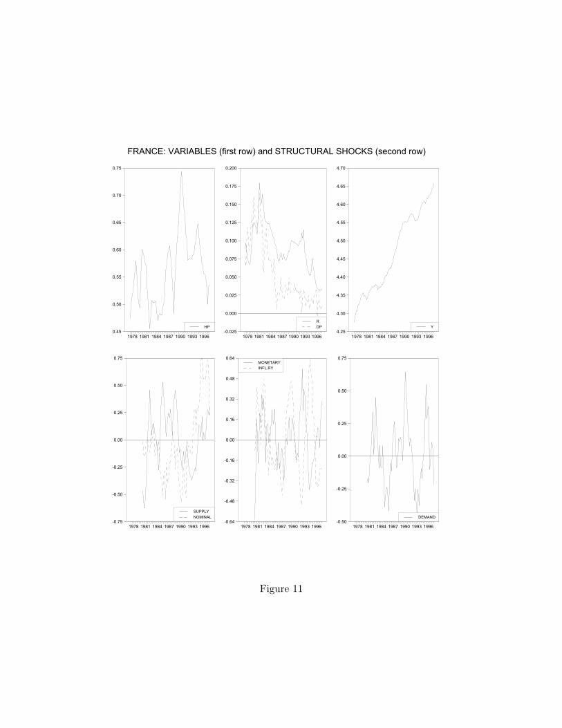
Figure 11

FRANCE: VARIABLES (first row) and STRUCTURAL SHOCKS (second row)

1978 1981 1984 1987 1990 1993 19960.45

0.50

0.55

0.60

0.65

0.70

0.75

HP

1978 1981 1984 1987 1990 1993 1996-0.75

-0.50

-0.25

0.00

0.25

0.50

0.75

SUPPLYNOMINAL

1978 1981 1984 1987 1990 1993 1996-0.025

0.000

0.025

0.050

0.075

0.100

0.125

0.150

0.175

0.200

RDP

1978 1981 1984 1987 1990 1993 1996-0.64

-0.48

-0.32

-0.16

0.00

0.16

0.32

0.48

0.64MONETARYINFL.RY

1978 1981 1984 1987 1990 1993 19964.25

4.30

4.35

4.40

4.45

4.50

4.55

4.60

4.65

4.70

Y

1978 1981 1984 1987 1990 1993 1996-0.50

-0.25

0.00

0.25

0.50

0.75

DEMAND

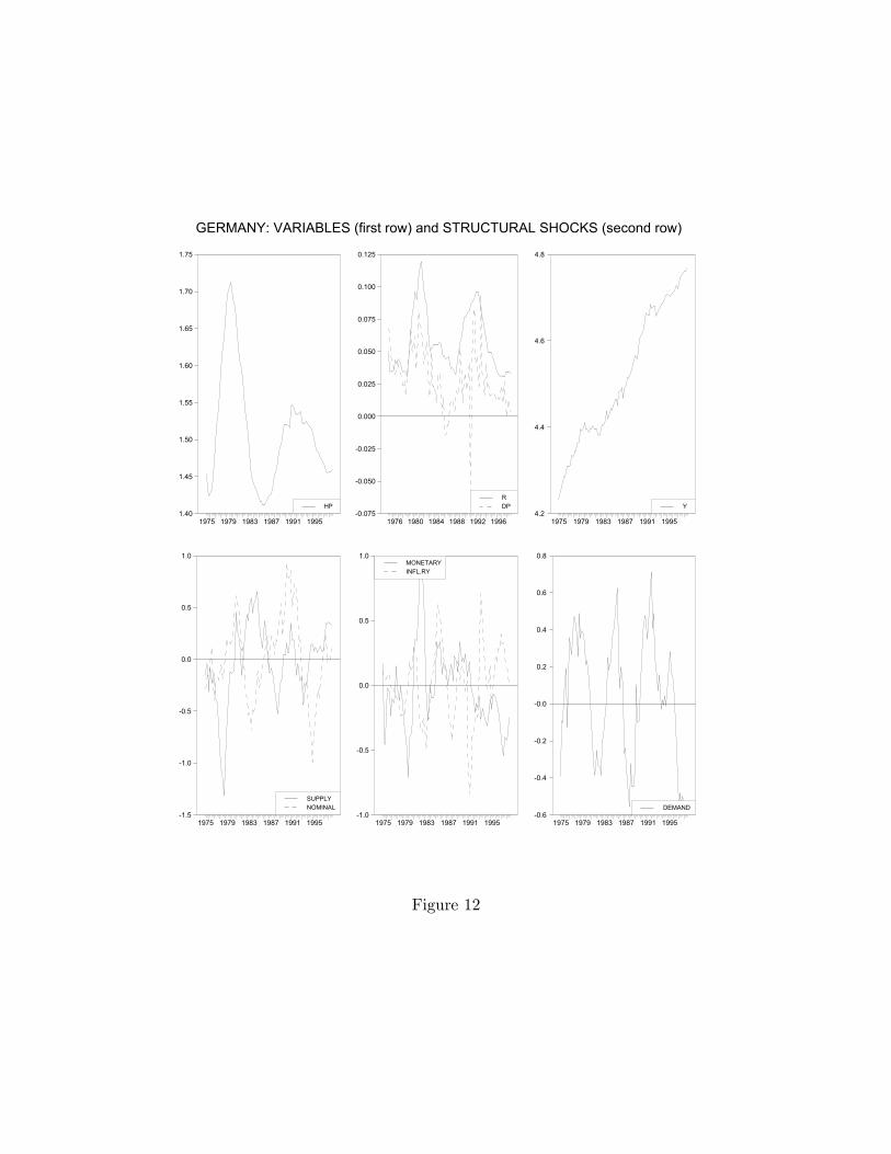
Figure 12

GERMANY: VARIABLES (first row) and STRUCTURAL SHOCKS (second row)

1975 1979 1983 1987 1991 19951.40

1.45

1.50

1.55

1.60

1.65

1.70

1.75

HP

1975 1979 1983 1987 1991 1995-1.5

-1.0

-0.5

0.0

0.5

1.0

SUPPLYNOMINAL

1976 1980 1984 1988 1992 1996-0.075

-0.050

-0.025

0.000

0.025

0.050

0.075

0.100

0.125

RDP

1975 1979 1983 1987 1991 1995-1.0

-0.5

0.0

0.5

1.0MONETARYINFL.RY

1975 1979 1983 1987 1991 19954.2

4.4

4.6

4.8

Y

1975 1979 1983 1987 1991 1995-0.6

-0.4

-0.2

-0.0

0.2

0.4

0.6

0.8

DEMAND

Figure 13

ITALY: VARIABLES (first row) and STRUCTURAL SHOCKS (second row)

1973 1977 1981 1985 1989 1993 1997-0.48

-0.32

-0.16

0.00

0.16

0.32

HP

1973 1977 1981 1985 1989 1993 1997-0.75

-0.50

-0.25

0.00

0.25

0.50

0.75

1.00

SUPPLYNOMINAL

1973 1977 1981 1985 1989 1993 19970.00

0.05

0.10

0.15

0.20

0.25

0.30

RDP

1973 1977 1981 1985 1989 1993 1997-0.75

-0.50

-0.25

0.00

0.25

0.50

0.75MONETARYINFL.RY

1973 1977 1981 1985 1989 1993 19975.2

5.3

5.4

5.5

5.6

5.7

5.8

5.9

Y

1973 1977 1981 1985 1989 1993 1997-0.75

-0.50

-0.25

0.00

0.25

0.50

0.75

DEMAND

Figure 14

SPAIN: VARIABLES (first row) and STRUCTURAL SHOCKS (second row)

1987 1989 1991 1993 1995 19976.65

6.72

6.79

6.86

6.93

7.00

7.07

7.14

7.21

HP

1987 1989 1991 1993 1995 1997-1.5

-1.0

-0.5

0.0

0.5

1.0

1.5

SUPPLYNOMINAL

1987 1989 1991 1993 1995 19970.000

0.025

0.050

0.075

0.100

0.125

0.150

RDP

1987 1989 1991 1993 1995 1997-1.25

-1.00

-0.75

-0.50

-0.25

0.00

0.25

0.50

0.75

1.00MONETARYINFL.RY

1987 1989 1991 1993 1995 19974.360

4.400

4.440

4.480

4.520

4.560

4.600

4.640

4.680

4.720

Y

1987 1989 1991 1993 1995 1997-1.25

-1.00

-0.75

-0.50

-0.25

0.00

0.25

0.50

0.75

1.00

DEMAND

Figure 15

SWEDEN: VARIABLES (first row) and STRUCTURAL SHOCKS (second row)

1979 1982 1985 1988 1991 1994 1997-4.88

-4.80

-4.72

-4.64

-4.56

-4.48

-4.40

-4.32

HP

1979 1982 1985 1988 1991 1994 1997-0.8

-0.6

-0.4

-0.2

-0.0

0.2

0.4

0.6

SUPPLYNOMINAL

1979 1982 1985 1988 1991 1994 1997-0.05

0.00

0.05

0.10

0.15

0.20

0.25

RDP

1979 1982 1985 1988 1991 1994 1997-0.50

-0.25

0.00

0.25

0.50

0.75MONETARYINFL.RY

1979 1982 1985 1988 1991 1994 19974.30

4.35

4.40

4.45

4.50

4.55

4.60

4.65

4.70

Y

1979 1982 1985 1988 1991 1994 1997-0.75

-0.50

-0.25

0.00

0.25

0.50

DEMAND

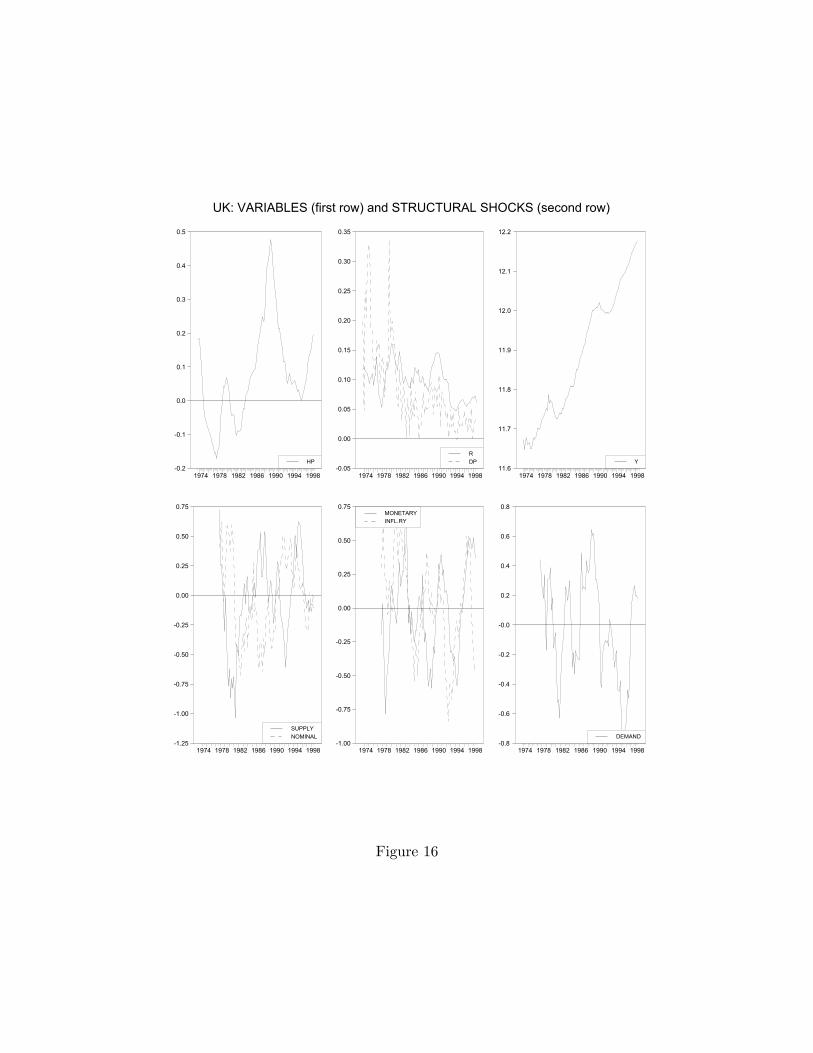
Figure 16

UK: VARIABLES (first row) and STRUCTURAL SHOCKS (second row)

1974 1978 1982 1986 1990 1994 1998-0.2

-0.1

0.0

0.1

0.2

0.3

0.4

0.5

HP

1974 1978 1982 1986 1990 1994 1998-1.25

-1.00

-0.75

-0.50

-0.25

0.00

0.25

0.50

0.75

SUPPLYNOMINAL

1974 1978 1982 1986 1990 1994 1998-0.05

0.00

0.05

0.10

0.15

0.20

0.25

0.30

0.35

RDP

1974 1978 1982 1986 1990 1994 1998-1.00

-0.75

-0.50

-0.25

0.00

0.25

0.50

0.75MONETARYINFL.RY

1974 1978 1982 1986 1990 1994 199811.6

11.7

11.8

11.9

12.0

12.1

12.2

Y

1974 1978 1982 1986 1990 1994 1998-0.8

-0.6

-0.4

-0.2

-0.0

0.2

0.4

0.6

0.8

DEMAND