
House Allocation with Overlapping Agents: A … Tim Hister and seminar participants at the...
41
JENA ECONOMIC RESEARCH PAPERS # 2009 – 075 House Allocation with Overlapping Agents: A Dynamic Mechanism Design Approach by Morimitsu Kurino www.jenecon.de ISSN 1864-7057 The JENA ECONOMIC RESEARCH PAPERS is a joint publication of the Friedrich Schiller University and the Max Planck Institute of Economics, Jena, Germany. For editorial correspondence please contact [email protected]. Impressum: Friedrich Schiller University Jena Max Planck Institute of Economics Carl-Zeiss-Str. 3 Kahlaische Str. 10 D-07743 Jena D-07745 Jena www.uni-jena.de www.econ.mpg.de © by the author.
Transcript of House Allocation with Overlapping Agents: A … Tim Hister and seminar participants at the...

JENA ECONOMIC RESEARCH PAPERS
# 2009 – 075
House Allocation with Overlapping Agents: A Dynamic Mechanism Design Approach
by
Morimitsu Kurino
www.jenecon.de
ISSN 1864-7057
The JENA ECONOMIC RESEARCH PAPERS is a joint publication of the Friedrich Schiller University and the Max Planck Institute of Economics, Jena, Germany. For editorial correspondence please contact [email protected]. Impressum: Friedrich Schiller University Jena Max Planck Institute of Economics Carl-Zeiss-Str. 3 Kahlaische Str. 10 D-07743 Jena D-07745 Jena www.uni-jena.de www.econ.mpg.de © by the author.

House Allocation with Overlapping Agents:
A Dynamic Mechanism Design Approach ∗
Morimitsu Kurino †
This version: September 2009
Abstract
Many real-life applications of house allocation problems are dynamic. For example, in
the case of on-campus housing for college students, each year freshmen apply to move in
and graduating seniors leave. Each student stays on campus for a few years only. A student
is a “newcomer” in the beginning and then becomes an “existing tenant.” Motivated by this
observation, we introduce a model of house allocation with overlapping agents. In terms
of dynamic mechanism design, we examine two representative static mechanisms of serial
dictatorship (SD) and top trading cycles (TTC), both of which are based on an ordering
of agents and give an agent with higher order an opportunity to obtain a better house.
We show that for SD mechanisms, the ordering that favors existing tenants is better than
the one that favors newcomers in terms of Pareto efficiency. Meanwhile, this result holds
for TTC mechanisms under time-invariant preferences in terms of Pareto efficiency and
strategy-proofness. We provide another simple dynamic mechanism that is strategy-proof
and Pareto efficient.
Keywords: house allocation, overlapping agents, dynamic mechanism, top trading cycles,
serial dictatorship
JEL classification: C71; C78; D71; D78
∗This paper is based on Chapter 4 of my Ph.D. dissertation submitted to the University of Pittsburgh. I
am very grateful to M. Utku Unver for his guidance, support, and discussions. I am also grateful to Andreas
Blume, Oliver Board, Sourav Bhattacharya, Onur Kesten, and Ted Temzelides for their guidance and to Lars
Ehlers, Tim Hister and seminar participants at the University of Bonn, the Max Plank Institute of Economics,
and Sophia University for discussions. All errors are my responsibility.†Max Planck Institute of Economics, Jena, Germany. Email: [email protected]
Jena Economic Research Papers 2009 - 075

1 Introduction
The static allocation problem1 of assigning indivisible goods, called “houses,” to agents without
monetary transfers has been extensively studied and applied to real-life markets such as on-
campus housing for college students (cf. Abdulkadiroglu Sonmez, 1999; Chen and Sonmez,
2002; Guillen and Kesten, 2008), kidney exchanges for patients (Roth, Sonmez, and Unver
2004), and school choice for U.S. public schools (cf. Abdulkadiroglu and Sonmez, 2003). Until
now, there has been little attempt to analyze dynamic house allocations problems.2
Considering dynamic aspects enables us to explain aspects of the allocation problem that
cannot be captured by static models. For example, in the case of on-campus housing for college
students, each year freshmen apply to move in and graduating seniors leave. Each student stays
on campus for a few years only. A student is a “newcomer” in the beginning and then becomes
an “existing tenant.” In general, students are overlapping. In this structure, it is not always
dynamically Pareto efficient to have a static Pareto efficient allocation in each period.
To illustrate this point, suppose in the first period t = 1, there is one agent a0, called
an initial existing tenant,3 who came before the market starts and lives only in this period.
Moreover, in each period t ≥ 1, one agent at comes to live in a house in periods t and t+ 1. In
each period t, there is an existing tenant at−1 who came in the previous period, and a newcomer
at. There are two durable houses ℎ1 and ℎ2 available. Each agent prefers ℎ1 to ℎ2, and (ℎ2, ℎ1)
to (ℎ1, ℎ2).4 Consider the allocation:
t = 1 t = 2 t = 3 t = 4 ⋅ ⋅ ⋅a0 ℎ2
a1 ℎ1 ℎ2
a2 ℎ1 ℎ2
a3 ℎ1 ℎ2...
......
1See Sonmez and Unver (2008) for a recent survey.2See recent exceptions: Abdulkadiroglu and Loertscher (2007), Bloch and Cantala (2008), and Unver (2009).3Throughout this paper, the terminology “existing tenants” indicates the agents who came to the market in
the previous period. It does not always mean that they have property rights for houses, unlike the ones used by
Abdulkadiroglu and Sonmez(1999).4For example, (ℎ2, ℎ1) is a consumption path where an agent consumes house ℎ2 in the first period, and ℎ1
in the next. Note that this preference violates the discounted utility model. However, considering a critique of
the discount utility model as reviewed by Frederick, Lowenstein, and O’Donoghue (2002), we allow for any strict
preference relation on {ℎ1, ℎ2} × {ℎ1, ℎ2} in this paper. See footnote 15 for a further discussion.
1
Jena Economic Research Papers 2009 - 075

In each period, an existing tenant is assigned ℎ2 and a newcomer is assigned ℎ1. This allocation is
Pareto efficient for each period’s static market. However, consider an infinite exchange between
an exiting tenant and a newcomer in each period where an existing tenant exchanges her house
ℎ2 for the newcomer’s house ℎ1. As a result, the initial existing tenant is assigned ℎ1, and each
of the other agents is assigned (ℎ2, ℎ1). This new allocation is preferred to the original by every
agent. Thus, the original allocation is not dynamically Pareto efficient.
Many universities in the United States use a variant of the random serial dictatorship mech-
anism to allocate dormitory rooms.5 This mechanism randomly orders the agents and then
applies the serial dictatorship (SD) mechanism: the first agent is assigned her top choice, and
the next agent is assigned her top choice among the remaining rooms, and so on. This ordering
is not entirely random, but rather depends on seniority. That is, existing tenants are favored
over newcomers.
In the previous example, consider period orderings which order a newcomer at as the first
and an existing tenant at−1 as the second in each period. Running an SD mechanism in each
period, we obtain the same allocation as indicated in the previous table. As we saw, this
outcome is not dynamically Pareto efficient. On the other hand, consider other period orderings
that order an existing tenant first, and a newcomer next. The allocation by the SD mechanism
with orderings that favor existing tenants over newcomers Pareto dominates the original, and
is dynamically Pareto efficient. That is, the ordering based on seniority performs well in terms
of Pareto efficiency.
The subject of this paper is to present a new dynamic framework for a house allocation
problem by considering overlapping agents,6 and to analyze the impact of orderings on Pareto
efficiency and strategy-proofness.7 To our knowledge, the existing literature takes orderings as
given, and we are the first to examine the importance of seniority-based mechanisms.
Our model extends the standard overlapping generations (OLG) models8 to a house alloca-
tion problem. Time is discrete and lasts forever. There are a finite number of durable houses
that are collectively owned by some institution, say a housing office. In each period, a finite
number of newcomers arrive and then stay for a finite number of periods, T , while the oldest
agents leave the market. Each agent consumes one house in each period. Each agent has a
5We will list some of real-life examples later in this section.6Block and Cantala (2008) independently consider a similar model to ours. One of the difference is that in
their model only one agent arrives in each period. See the Related literature section for a further discussion.7By strategy-proofness, all agents find it best to report true preferences.8See Samuelson (1958), or Ljungqvist and Sargent (2004).
2
Jena Economic Research Papers 2009 - 075

time-separable preference over houses that spans T periods, consisting of T period preferences.
Her given preference does not vary across time. That is, her type is drawn as a preference when
she arrives, but her type does not change over time. However, we do allow period preferences
to vary across periods. Only initial existing tenants who arrived before the market starts may
have endowments. In this environment, a housing office needs to find a mechanism to allocate
houses to agents. Unlike in a static model, the office is not able to elicit the preferences of
agents who will arrive in the future. In each period, the office assigns houses to agents present
in the market, and may assign property rights for the future as well as the current assignment.
Thus, the office takes into account the previous assignments in order to determine a current
assignment. Hence, the office faces a dynamic mechanism design problem.
We study two dynamic mechanisms. The first is a spot mechanism where in each period
a housing office asks agents present in that period about the current period preference, and
not the preference over all time periods. In particular, we look at spot mechanisms with or
without property rights transfer: In a spot mechanism with property rights transfer, the houses
occupied by the oldest agent become vacant in the next period, but those occupied by the other
agents become their endowment. On the other hand, a spot mechanism without property rights
transfer has no such transfer. Another dynamic mechanism is a futures mechanism in which
each new agent is asked to reveal her preference over all time periods when she arrives.
At any point of time, our spot mechanism without property rights transfer resembles a
house allocation problem (Hylland and Zeckhauser, 1979). A random serial dictatorship (RSD)
(static) mechanism has been studied (Abdulkadiroglu and Sonmez, 1998). Some colleges such
as Davidson College, Lafayyett College, and St. Olaf College use a seniority-based RSD spot
mechanism on the condition that all students are forced to participate in the mechanism every
year. As we saw in the previous example, in an SD spot mechanism (period orderings are given
each period), period orderings that favor existing tenants induce a Pareto efficient allocation
(Theorem 2). On the other hand, period orderings that favor newcomers do not always induce
a Pareto efficient allocation (Theorem 3).
Although it is simple, Pareto efficient, and strategy-proof (Svensson, 1994), the RSD mech-
anism is rarely used. Rather, many universities use a modified version of this mechanism, called
a RSD mechanism with squatting rights, where existing tenants either keep their current rooms,
or give up them and participate in the RSD mechanism. The main reason9 is that universi-
9James Earle, Assistant Vice Chancellor for Business at the University of Pittsburgh, gave me the following
official reason: The goal of the Department of Housing is first and foremost, customer satisfaction. By allowing
students the opportunity to retain a room they like, we are guaranteeing the satisfaction of these returning
3
Jena Economic Research Papers 2009 - 075

ties want to keep students on campus, which makes the universities financially less risky. This
seniority-based mechanism is used in Northwestern University, University of Michigan, and the
University of Pittsburgh, among others. Students in these colleges can choose stay off-campus.
Even colleges that require all students to live on campus use this seniority-based mechanism;
for example, Godrdon College, Guilford College, Lawrence University. Although it is ex ante
individually rational, this mechanism is not Pareto efficient (Abdulkadiroglu and Sonmez, 1999),
and not ex post individually rational (Some students who participate in the RSD mechanism
may get a worse room than their previously owned one.).
The RSD mechanism with squatting rights motivates us to introduce a spot mechanism with
property rights transfer where, in each period, the houses occupied by the oldest agents become
vacant in the next period, but those occupied by the other agents are inherited as property
rights or endowments in the next period. At any one point of time, this spot mechanism
resembles a static house allocation problem with existing tenants (Abdulkadiroglu and Sonmez,
1999) in which there are newcomers (agents with no endowments) and existing tenants (agents
with endowments). In a static context, since the SD with squatting rights is not Pareto efficient,
Abdulkadiroglu and Sonmez (1999) propose a mechanism based on the top trading cycles (TTC)
mechanism (Shapley and Scarf, 1974), referred to as AS-TTC mechanism. This mechanism
restores Pareto efficiency that the RSD mechanism with squatting rights lacks, while satisfying
individual rationality and strategy-proofness.
We introduce a notion of acceptability in which each agent is made weakly better off as
time goes on. This corresponds to the situation, in a spot mechanism with property rights
transfer, where the static mechanism in each period is individually rational. Thus, it can be
seen as a counterpart of individual rationality in a static problem. As we mentioned, in order to
keep students on campus, many universities give property rights to students. In this sense, the
acceptability is desirable for dynamic mechanisms. However, we prove an Impossibility Theorem
where there is no dynamic mechanism that is Pareto efficient and acceptable (Theorem 1).
Any SD spot mechanism is not acceptable, since all houses that an existing tenant weakly
prefers to their previously occupied one can be obtained by agents with higher order. However,
since an AS-TTC static mechanism is individually rational, we consider a TTC spot mechanism
in which an AS-TTC static mechanism is run each period in a spot mechanism with property
customers. Furthermore, if these students were forced out of their room, they could not only become a dissatisfied
customer, if they then get a room they don’t like, but they could also decide to live off campus and become
someone else’s customer. Why risk the loss of revenue, when you have the potential to have a satisfied customer
simply by allowing them to retain their room?
4
Jena Economic Research Papers 2009 - 075

rights transfer. Since an AS-TTC mechanism is individually rational, a TTC spot mechanism
is acceptable. However, by the Impossibility Theorem, this spot mechanism is not Pareto
efficient.10 We restrict the preference domain to time-invariant preferences where each agent
has preference consisting of identical period preferences. We emphasize that this is not just a
repetition of an AS-TTC static mechanism but has two distinct features. First, we have entry
and exit of agents with different preferences in each period. Second, endowments or property
rights are endogenous. Under time-invariant preferences, we show that period orderings that
favor existing tenants perform better than the ones that favor newcomers in terms of Pareto
efficiency and strategy-proofness (Theorems 5, 6, 7 and 8).
Finally, we propose a serial dictatorship (SD) futures mechanism which is based on orderings
of agents. We show that it is strategy-proof and Pareto efficient.
1.1 Related literature
There is an extensive literature on static house allocation problems. See Sonmez and Unver
(2008) for a recent and comprehensive survey.
A dynamic house allocation problem can be classified depending on how and when agents
arrive and exit. But with the deterministic arrival and exit of agents, Bloch and Cantala (2008)
independently consider a model similar to ours. There are several differences that distinguish
our work from theirs. First, in their model only one agent enters and exits the market in
each period, while our model allows for any finite number of agents to enter and exit. Second,
in their model the type of an entering agent is drawn as a period preference but does not
vary as time goes on, while in our model we allow period preferences to vary across periods.
Third, their preference domain is more restricted than ours. They consider two cases: 1) all
agents have identical preferences, and 2) agents have heterogenous preferences but the surpluses
from matchings are supermodular. They analyze a Markovian assignment mechanism with
property rights transfer that is acceptable. Their seniority-rule corresponds to our constant SD
spot mechanism favoring existing tenants (to be defined in section 4) in a specific environment
as described above. However, they do not look at how static mechanisms such as a serial
dictatorship mechanism or a TTC mechanism behave in a dynamic setting. They characterize
the independent convergent rule when agents are homogenous, but do not consider incentive
issues.
10Note that in the general preference domain a TTC spot mechanism is not dynamically but statically Pareto
efficient. An SD mechanism with squatting rights is not even statically Pareto efficient.
5
Jena Economic Research Papers 2009 - 075

Unver(2009) studies a dynamic mechanism design with an application to kidney exchange
for patients (Roth, Sonmez, and Unver, 2004) in which agents arrive stochastically. However,
our dynamic model cannot be applied to kidney exchange for two reasons. First, a patient with
live donors (i.e. an agent with an endowment) arrives in each period, while in our model only
initial existing tenants may have endowments. Second, kidney patients immediately leave the
market once their exchange is done, but our model does not allow for this.
Additionally, Abdulkadiroglu and Loertscher (2007) consider a dynamic problem without
the arrival and exit of agents and with two periods in which each agent’s type is drawn in each
period. They also introduce a dynamic mechanism that depends on the first period allocation,
and examine efficiency and optimal dynamic mechanisms. Similarly, the case of multiple-type
(static) housing markets, where multiple types of indivisible goods are traded and endowments
are given, can be seen as a dynamic house allocation problem with finite horizon the length of
which is the same as the number of types. Konishi, Quint and Wako (2001) obtain a negative
result in which there is no mechanism that is Pareto efficient, individually rational, and strategy-
proof.
Although there are almost no papers on how important the ordering of agents is in a mecha-
nism, Sonmez and Unver (2005) show that a stochastic AS-TTC mechanism favoring newcomers
is equivalent to the core-based mechanism in a static house allocation with exiting tenants.
Finally, there is a growing literature on dynamic mechanism design with monetary transfers.
For example, see Athey and Segal (2007) and Gershkov and Moldovanu (2009).
2 The Model
2.1 A dynamic problem
Time is discrete, starts at t = 1 and lasts forever. There is a finite set, H, of indivisible goods,
called houses, which are collectively owned by some institution (say a housing office.). The
houses are perfectly durable in that they can be used in each period. The number of available
houses is fixed throughout time.
Agents live in houses for T periods, where T ≥ 2 is finite.11 An agent who came before the
11If T = 1, then our model has a different static model in each period, so there is no dynamic issue. Thus, we
exclude T = 1.
6
Jena Economic Research Papers 2009 - 075

Table 1: Demographic structures
1 2 ⋅ ⋅ ⋅ T − 1 T ⋅ ⋅ ⋅ t t+ 1 ⋅ ⋅ ⋅ t+ T − 2 t+ T − 1
a2−Ti ✓
a3−Ti ✓ ✓...
......
. . .
a0i ✓ ✓ ⋅ ⋅ ⋅ ✓
a1i ✓ ✓ ⋅ ⋅ ⋅ ✓ ✓...
. . .
at−T+1i ✓
at−T+2i ✓ ✓
......
.... . .
at−1i ✓ ✓ ⋅ ⋅ ⋅ ✓
ati ✓ ✓ ⋅ ⋅ ⋅ ✓ ✓...
Note: The mark “✓” indicates when a newcomer a�i in period � is in the market with the corresponding period
in the first row.
model starts is called an initial existing tenant.12 In particular, an initial existing tenant
who came at period � ≤ 0 is called a newcomer in period � , and lives in one house in each
period from period 1 to � + T − 1. For example, an oldest agent in period 1 is a newcomer in
period 2− T , and lives in a house only in period 1. In each period t ≥ 1, newcomers arrive to
live in a house in every period from period t to t+T −1. Each such agent is called a newcomer
in period t. The number of newcomers in each period t ≥ 2 − T is finite, and is denoted by
n. Let N(t) := {at1, at2, ⋅ ⋅ ⋅ , atn} be the set of newcomers in period t ≥ 2− T .13 Table 2.1 shows
the demographic structure of our model. Note that there are both an infinite number of periods
and an infinite number of agents in this model. This “double infinity” is the major source of
the theoretical peculiarities of the OLG model (Shell, 1971).
In each period t ≥ 1, agents in the market are newcomers in periods t − T + 1, t + T +
1, ⋅ ⋅ ⋅ , t− 1, t. Agents who came before period t are also called existing tenants in period t.
That is, they are newcomers in periods t− T + 1, ⋅ ⋅ ⋅ , t− 1. Let E(t) be the set of all existing
tenants in period t. Thus, E(t) ≡ ∪{N(�) : t − T + 1 ≤ � ≤ t − 1} and E(1) is the set of all
12See footnote 3.13A variable indexed by (t) is defined only in period t.
7
Jena Economic Research Papers 2009 - 075

initial existing tenants. Moreover, let A(t) := N(t) ∪ E(t) be the set of all agents present in
period t ≥ 1. Note ∣A(t)∣ = nT . We assume that the number of houses is equal to the number
of agents present in each period; that is, ∣H∣ = ∣A(t)∣ = nT . Throughout this paper, we fix the
sets H and A(t) for each t ≥ 1.
For notational simplicity, we introduce a virtual house, ℎ0, which can be assigned to
any number of agents. Later we will need to keep track of property rights or endowments
assigned in each period. The virtual house will be used to assign no endowment to agents. Let
H := H ∪ {ℎ0}. To distinguish houses in H from the virtual house, we call a house in H a real
house.
A period t matching, �(t), is an assignment of houses to agents in A(t) such that each
agent is assigned one (real or virtual) house and only the virtual house ℎ0 can be assigned to
more than one agent in period t ≥ 1. For each a in A(t), we refer to �a(t) as the period t
assignment of agent a under �(t). Letℳ(t) be the set of all period t matchings. A matching
plan is a collection of period t matchings from period 1 on, denoted by � := {�(t)}∞t=1. For each
a in A(t), we refer to �a := (�a(t), �a(t + 1), ⋅ ⋅ ⋅ , �a(t + T − 1)) as the assignment of agent a
under �. Let ℳ be the set of all matching plans.
Each initial existing tenant, a, in N(t) has a strict preference relation, Ra, on the product
HT+t−1. In other words, Ra is a linear order over HT+t−1.14 Given assignments �a and �a,
�aRa �a means that agent a weakly prefers �a to �a, and �a Pa �a means that agent a strictly
prefers �a to �a under Ra. On the other hand, a newcomer in period t ≥ 1 has a strict preference
relation, Ra, on the product HT . In addition, we assume that each agent has a time-separable
preference defined as follows:15
Definition 1. A preference, Ra, of newcomer a in period t ≥ 1 is time-separable if for each
� = t, ⋅ ⋅ ⋅ , T + t−1, there exist strict preferences Ra(�) on H such that for any two assignments
�1a and �2
a on HT ,
if ∀� = t, ⋅ ⋅ ⋅ , t+ T − 1, �1a(�)Ra(�)�2
a(�) and ∃� , �1a(�)Pa(�)�2
a(�), then �1a Pa �
2a.
The above definition is similarly defined for initial existing tenants. Moreover, Ra(�) is called
14A linear order is a complete, reflexive, transitive, and antisymmetric binary relation.15As we discussed in the Introduction, our assumption of time-separable strict preference violates the dis-
counted utility (DU) model in two ways. Even if her preference is time-invariant, an agent may prefer improving
path of houses over declining paths, which violates the DU model. If not so, a period preference in some period
may be affected by houses experienced in prior or future periods, which violates the independence assumption
of the DU model. We do not go into details of experimental results on the validity of these assumptions. See
Frederick, Lowenstein, and O’Donoghue (2002), especially section 4.2.4 and 4.2.5, for further discussions.
8
Jena Economic Research Papers 2009 - 075

a period � preference. A preference is called time-invariant if all period preferences are
identical.
The time-separability condition means that preferences between houses in the same period
do not depend on the assignment of houses in the other periods. Moreover, we assume that the
virtual house is the worst choice for any period preference of each agent.
We write �aRa �′a as �Ra �
′ when no confusion arises. Let ℛa be the set of all preference
relations of agent a, and ℛ :=∏{ℛa : a ∈ A} be the set of all preference profiles. Let ℛa(�)
be the set of all period � preferences of agent a, and ℛ(�) :=∏{ℛa(�) : a ∈ A(�)} be the set
of all period preference profiles for agents present in period � .
An endowment profile is expressed by a matching plan e := {ea}a∈A ∈ℳ. An endowment
of each agent except the initial existing tenants consists only of the virtual house. We consider
two cases: 1) each initial existing tenant has an endowment consisting only of the virtual
house, 2) each initial existing tenant has the right to live in one real house only in period
1; that is, ea = (ℎ, ℎ0, ⋅ ⋅ ⋅ , ℎ0) for some real house ℎ and for the virtual house ℎ0. A house
allocation problem with overlapping agents or simply, a dynamic problem is expressed
by (A,H,R, e). The first case (second case) in the above is called a dynamic problem without
endowments (with endowments). The problem with endowments is considered for a specific
mechanism.16 Unless stated explicitly, a dynamic problem is either with or without endowments.
Throughout this paper, we fix A, H.
As we discussed in the Introduction, instead of the pure RSD mechanism, many universities
introduce squatting rights in that existing tenants have the right to extend their lease in order
to make on-campus housing more attractive. This motivates the following:
Definition 2. In a dynamic problem without endowments, a matching plan {�(t)}∞t=1 is ac-
ceptable if each agent is better off as time goes on. That is:
1. ∀t if 2− T ≤ t ≤ 0, ∀a ∈ N(t), ∀� = t+ 1, ⋅ ⋅ ⋅ , t+ T − 1, �(�)Ra(�)�(� − 1), and
2. ∀t ≥ 1, ∀a ∈ N(t), ∀� = t+ 1, ⋅ ⋅ ⋅ , t+ T − 1, �(�)Ra(�)�(� − 1).
For a dynamic problem with endowments, it is acceptable if the above conditions hold and
each initial existing tenant is assigned a house that is at least as good as her endowment in
period 1, i.e., ∀a ∈ E(1), �(1)Ra(1) e(1).
16The specific mechanism is a spot mechanism with property rights transfer.
9
Jena Economic Research Papers 2009 - 075
The first condition is for initial existing tenants, and the second is for the other agents.
A matching plan is Pareto efficient (PE) if there is no other matching plan that makes
all agents weakly better off and at least one agent strictly better off.
3 Dynamic Mechanisms
At any given time, the housing office is not able to ask newcomers who will arrive in the future
about their preference. In order to reflect preferences, the office cannot determine the houses
from the beginning to the future at once. Instead, it determines the assignment in each period.
This feature brings about new aspects for mechanism design problems. First, message spaces
can take many forms even if we focus on direct mechanisms. For example, in each period,
the office can ask an agent about her corresponding period preference or her entire preference.
Second, in each period, the office can assign not only the houses for the current period but also
houses for the future. Finally, in any given period, some of the houses are already assigned, and
thus the office has to take into account this past assignment in order to decide on the current
assignment.
Generally, for a dynamic problem with or without endowments, a dynamic mechanism is
a function Π : ℛ →ℳ that determines a matching plan for each preference profile. A dynamic
mechanism is acceptable if it always selects an acceptable matching plan. Moreover, it is
Pareto efficient if it always selects a Pareto efficient matching plan.
We restrict attention to two dynamic mechanisms. The first is a spot mechanism where,
in each period, the office asks each agent present in the period to reveal her corresponding
period preference. We also consider a futures mechanism. In the first period the office asks
all agents present in this period (i.e. initial existing tenants and newcomers in period 1) about
their preference. In subsequent periods, the office asks newcomers about their entire preference.
3.1 Spot mechanisms
We formally define a spot mechanism by introducing the concepts of a static problem and a
static mechanism.
10
Jena Economic Research Papers 2009 - 075
3.1.1 Static mechanisms
Fix a dynamic problem with or without endowments, (A,H,R, e). Consider a period t ≥ 1.
A period t static problem is defined as (D(t), U(t), H,R(t), e(t)).17 An agent a in D(t) is
called an endowed agent and occupies a real house, ea(t), while an agent in U(t) is called an
unendowed agent and does not have the right to live in any real house. Thus, agents in A(t)
are either endowed or unendowed, that is, A(t) ≡ D(t) ∪ U(t). A real house is called vacant if
it is not occupied by any endowed agent. Moreover, R(t) is a strict preference profile of agents
in A(t), and e(t) is the endowment profile of agents in A(t).
In such models, if D(t) = ∅ and U(t) = A(t), a static problem is a house allocation problem
(Hylland and Zeckhauser, 1979). If D(t) = A(t) and U(t) = ∅, it is a housing market (Shapley
and Scarf, 1974). Finally, if D(t) ∕= ∅, U(t) ∕= ∅, and D(t)∪U(t) = A(t), it is a house allocation
problem with existing tenants (Abdulkadirogle and Somez, 1999).
In a static problem where there are endowed agents, a matching is individually rational
if no endowed agent strictly prefers her endowment to her assignment. A matching is Pareto
efficient if there is no other matching that makes all agents weakly better off and at least one
agent strictly better off.
A period t static mechanism determines a period t matching for each of both a period
preference profile and an endowment profile. That is, it is a function t : ℛ(t)×ℳ(t)→ℳ(t).
It is denoted by t(R(t), e(t)) for each period preference profile, R(t), and each endowment
profile, e(t). A period t static mechanism is individually rational (Pareto efficient) if it
always selects an individually rational (Pareto efficient) period t matching. In addition, it
is strategy-proof if truth-telling is a weakly dominant strategy in its associated preference
revelation game.
3.1.2 Spot mechanisms without property rights transfer
In this section, we define a spot mechanism without property rights transfer. To make the mech-
anism consistent with the problem, we look only at a dynamic problem without endowments.
In this mechanism, D(t) = 0 and U(t) = A(t) for each t ≥ 1, we always have a static house
allocation problem in each period. This motivates the following definition:
Definition 3. Given a sequence of static mechanisms { t}∞t=1, a spot mechanism without
17Recall that a variable indexed by (t) is defined only in period t.
11
Jena Economic Research Papers 2009 - 075

property rights transfer, Π : ℛ → ℳ with R 7→ Π(R) := (Π(R; 1),Π(R; 2), ⋅ ⋅ ⋅ ) ∈ ℳ, is
obtained through static mechanisms as follows: for each period t ≥ 1,
Π(R; t) := t(R(t), e(t)),
where all e(t)’s consist of the virtual house.
3.1.3 Spot mechanisms with property rights transfer
Unlike in the previous mechanism, we consider the transfer of property rights in either a dynamic
problem with or without endowments. In each period, the houses occupied by the oldest agents
become vacant in the next period, but those occupied by the other agents are inherited as
property rights or endowments in the next period.
In a dynamic problem with endowments, we have ∀t ≥ 1, D(t) = E(t). That is, endowed
agents are the existing tenants. On the other hand, in a dynamic problem without endowments,
we have D(1) = ∅ and U(1) = A(1), but ∀t ≥ 2, D(t) = E(t). In other words, in the first
period, there is no endowed agent, but endowed agents are the existing tenants from the second
period on.
Definition 4. Given a sequence of static mechanisms { t}∞t=1, a spot mechanism with
property rights transfer, Π : ℛ → ℳ with R 7→ Π(R) := (Π(R; 1),Π(R; 2), ⋅ ⋅ ⋅ ) ∈ ℳ, is
obtained through static mechanisms as follows: for each preference profile R in ℛ,
1. In period 1,
Π(R; 1) ≡ �(1) := 1 (R(1), e(1)) .
2. In period t ≥ 2, set e(t) :=(�E(t)(t− 1), eN(t)(t)
),
Π(R; t) ≡ �(t) := t (R(t), e(t)) .
A spot mechanism is thus defined by using a sequence of static mechanisms. The link
between the period t− 1 static mechanism and the period t static mechanism is made possible
through the endogenous endowment e(t) for t ≥ 2. This makes it different from just a repetition
of a static mechanism. In each period, the current period mechanism depends on the previous
mechanism through the assigned endowment. More precisely, in period 1, the office faces a period
1 static market whose endowment corresponds to e(1) from the original dynamic problem. The
12
Jena Economic Research Papers 2009 - 075
office asks each agent a present in period 1 about her period 1 preference, Ra(1). Based on
the reported period preference profile, R(1), and the endowment, e(1), the office determines a
period 1 matching Π(R; 1) ≡ �(1) through the period 1 static mechanism, 1(R(1), e(1)). In
the next period, t = 2, each agent a who is still in the market (i.e., in E(2)) has the right to live
in the previously assigned house, �a(1). The agents’ endowment profile is �E(2)(1). Newcomers
in period 2 have the virtual endowment. Their endowment profile is eN(2)(2). Thus, we have
an endowment profile e(2) := (�E(2)(1), eN(2)(2)) for the period 2 static market. Based on
the reported period 2 preference profile, R(2), and the endowment, e(2), the office determines
a period 2 matching Π(R; 2) ≡ �(2) through the period 2 static mechanism, 2(R(2), e(2)).
Repeating this process produces the matching plan Π(R) ≡ {�(t)}∞t=1.
3.2 Strategy-proofness
Definition 5. A spot or futures mechanism Π : ℛ →ℳ is strategy-proof if
∀a ∈ A, ∀R ∈ ℛ, ∀R′a ∈ ℛa, Π(Ra, R−a)Ra Π(R′a, R−a).
Consider a spot mechanism. Agents face an extensive form with simultaneous moves. We are
interested in whether they reveal their true period preferences in each period static mechanism.
In any given period, revealing the true period preference for an agent does not depend on history,
but rather on that period alone. Implicit in the above definition is the restriction of our attention
to a class of history-independent strategies. That is, a spot mechanism is strategy-proof if,
for each agent, her history-independent strategy of revealing her true period preferences is
weakly better than any other history-independent strategy, regardless of the history-independent
strategies of the other agents.18
On the other hand, a futures mechanism is strategy-proof if truth-telling is a weakly domi-
nant strategy for each agent.
18In the definition of strategy-proofness in a static mechanism, truth-telling is a weakly dominant strategy
for each agent. However, to our knowledge, there is no existing definition of strategy-proofness investigated in
our dynamic setting. Instead of requiring truth telling to be a weakly dominant strategy for each agent, we
introduce a weaker notion by looking at a class of history-independent strategies in a spot mechanism.
13
Jena Economic Research Papers 2009 - 075

3.3 Impossibility result
In this section, we begin with a negative result. We will investigate positive results in later sec-
tions. First, we search for a dynamic mechanism that is Pareto efficient and strongly individually
rational. The following result rules out the existence of such a mechanism.
Theorem 1. Consider a dynamic problem with or without endowments. Suppose there are at
least two newcomers in each period who live for at least three periods. Then, there is no dynamic
mechanism that is Pareto efficient and acceptable.
Proof. First, we consider a dynamic problem without endowments. Pick two newcomers a11 and
a12 in period 1. Consider the case where agents live for three periods. Their period preferences
satisfy (from best to worst):
a11 a12Ra(1) Ra(2) Ra(3) Ra(1) Ra(2) Ra(3)
ℎ1 ℎ2 ℎ1 ℎ2 ℎ2 ℎ1
ℎ2 ℎ1 ℎ2 ℎ1 ℎ1 ℎ2
For example, ℎ1Ra11(1)ℎ2. Moreover,
a11 : (ℎ, ℎ2, ℎ2) ≻ (ℎ, ℎ1, ℎ1),
a12 : (ℎ, ℎ1, ℎ1) ≻ (ℎ, ℎ2, ℎ2),
where ℎ is any real house. Also, ℎ1 and ℎ2 are less preferred to the other houses for the agents
other than a11 and a12.
Seeking a contradiction suppose there is a Pareto efficient and acceptable matching plan
� ≡ {�(t)}∞t=1. First, by Pareto efficiency, in period 1, a11 is assigned ℎ1, and a12 is assigned ℎ2.
Then, in period 2, a12 is assigned ℎ2 from acceptability, and thus a11 is assigned ℎ1. Similarly, a11is assigned ℎ1 from acceptability, and thus a12 is assigned ℎ2. In summary, we have the following
matching plan.
�∣{a11,a12} t = 1 t = 2 t = 3
a11 ℎ1 ℎ1 ℎ1
a12 ℎ2 ℎ2 ℎ2
14
Jena Economic Research Papers 2009 - 075

Consider an exchange between a11 and a12 in periods 2 and 3. As a result, a11 is assigned
(ℎ1, ℎ2, ℎ2) and a12 is assigned (ℎ2, ℎ1, ℎ1). These assignments are strictly preferred by both
agents. Therefore, we have a contradiction.
In the other case where T > 2, we can include the previous case to obtain the result. For a
dynamic problem with endowments, let a11 own ℎ1 and a12 own ℎ2 in the first period. We can do
the same argument for this case.
4 Serial Dictatorship (SD) Spot Mechanisms
In this section, we consider a spot mechanism without property rights transfer for a dynamic
problem without endowments.
4.1 Definition
Since all of the mechanisms examined in this paper are based on an ordering of agents, here we
introduce various types of orderings. Given a set B ⊂ A of agents, an ordering in B is a linear
order, denoted by fB. We often denote it as the ordered list:
fB := (b1, b2, ⋅ ⋅ ⋅ , bm) if and only if b1 fB b2 fB ⋅ ⋅ ⋅ fB bm.
We say that b1 is the first agent in B, b2 is the second agent in B and so on. In addition,
agent a has higher order than agent b if a fB b. Specifically, we look at two kinds of
orderings. The first is a period t ordering, fA(t), which is an ordering of A(t), the set of all
agents present in period t ≥ 1. The second is cohort orderings fE(1) and fN(t) for t ≥ 1,
where fE(1) is an ordering of E(1) which is the set of all initial existing tenants, while fN(t) is
an ordering of N(t) which is the set of all newcomers in period t ≥ 1.
A serial dictatorship (SD) spot mechanism is a spot mechanism without property
rights transfer in which each period static mechanism is a serial dictatorship (SD) static
mechanism. An SD period t static mechanism is based on a period t ordering, fA(t), and is
defined as follows. Take any period t ordering, fA(t). Fix a preference profile, R(t). The first
agent gets her top choice, the second agent gets her top choice among houses excluding the one
assigned to the first agent. The kth agent gets her top choice among houses excluding those
assigned to all agents with higher order than her.
15
Jena Economic Research Papers 2009 - 075

It is known that an SD static mechanism is strategy-proof and Pareto efficient (Svensson,
1994). Note that an SD static mechanism is independent of the previously occupied houses. As
a result, an existing tenant is not guaranteed to obtain a house that is at least as good as her
occupied house in the previous period. Hence, an SD spot mechanism is not acceptable.
4.2 Strategy-proofness
We know that an SD static mechanism is strategy-proof and Pareto efficient. The question is
whether these properties hold for an SD spot mechanism.
Proposition 1. In a dynamic problem without endowments, an SD spot mechanism is strategy-
proof.
Proof. An SD spot mechanism has no transfer of property rights and consists of SD static
mechanisms, and thus each SD period mechanism is independent of the past assignments. Hence,
we have the desired result.
4.3 Pareto efficiency: some positive results
In a specific example in the Introduction, we demonstrated Pareto efficiency of an allocation
induced by an SD spot mechanism favoring existing tenants. In this subsection, we study under
what kind of period orderings the induced SD spot mechanism can achieve Pareto efficiency. To
this end, we introduce the following:
Definition 6. 1. A period t ordering fA(t) favors existing tenants if, in period t, each
existing tenant has higher order than any newcomer in fA(t). Moreover, it favors new-
comers if, in period t, each newcomer has higher order than any existing tenant in fA(t).
2. A sequence of period orderings favors existing tenants (newcomers) if, in each
period t, a period t ordering favors existing tenants (newcomers).
An SD spot mechanism induced by a sequence of period orderings favoring existing tenants
(newcomers) is called a SD spot mechanism favoring existing tenants (newcomers).
Definition 7. A sequence of period orderings is constant if the relative ranking of agents is
the same across periods. That is, if an agent, a, has higher order than another agent, a′, in
some period, then a has higher order than a′ in any other period when they are in the market.
16
Jena Economic Research Papers 2009 - 075

An SD spot mechanism induced by a constant sequence of period orderings is called a
constant SD spot mechanism. Now, we can state one of the main positive results.
Theorem 2. In a dynamic problem without endowments, a constant SD spot mechanism favor-
ing existing tenants is Pareto efficient.
Before proving the theorem, we explore the relation between the period orderings and the
cohort orderings for a given constant sequence of periods orderings favoring existing tenants.
The following example illustrates this.
Example. Consider a situation where there are two newcomers, at1 and at2, in each period
t ≥ −1. Agents live for three periods. Then, E(1) = {a−11 , a−12 , a01, a02}, N(t) = {at1, at2}, and
A(t) = N(t− 2) ∪N(t− 1) ∪N(t). Take a sequence {fA(t)}∞t=1 of period orderings such that
fA(1) =(a01, a
−11 , a02, a
−12 , a11, a
12
),
fA(2) =(a01, a
02, a
11, a
12, a
21, a
22
),
fA(3) =(a11, a
12, a
21, a
22, a
31, a
32
).
Notice that this sequence is constant and favors existing tenants. We can take the following
cohort orderings:
gE(1) = (a01, a−11 , a02, a
−12 ),
gE(1)∣A(2) = (a01, a02),
gN(t) = (at1, at2), for each t = 1, 2, 3.
Notice that
fA(1) = (gE(1), gN(1)),
fA(2) = (gE(1)∣A(2), gN(1), gN(2)),
fA(3) = (gN(1), gN(2), gN(3)).
The corresponding cohort orderings are denoted by using f instead of g.
In summary, we have the following lemma (the proof is straightforward).
Lemma 1. Given a constant sequence {fA(t)}∞t=1 of period ordering favoring existing tenants,
there are corresponding cohort orderings fE(1) and {fN(t)}t≥1 such that
fA(t) = (fE(1)∣A(t), fN(1), ⋅ ⋅ ⋅ , fN(t)), ∀t = 1, ⋅ ⋅ ⋅ , T − 1, and
fA(t) = (fN(t−T+1), ⋅ ⋅ ⋅ , fN(t)), ∀t ≥ T.
17
Jena Economic Research Papers 2009 - 075

Now we are ready to prove Theorem 2.
Proof of Theorem 2. Let {fA(t)}∞t=1 be given. From Lemma 1, let a sequence (fE(1), {fN(t)}∞t=1)
give the corresponding cohort orderings. Let � = {�(t)}∞t=1 be a matching plan generated by a
constant SD spot mechanism for some arbitrary preference profile R. To find a contradiction,
suppose some matching plan � Pareto dominates �. Then,
∀a ∈ A, �Ra � and ∃b ∈ A, �Pb �.
Since A = E(1) ∪ (∪∞t=1N(t)), either b ∈ E(1) or b ∈ N(t) for some t ≥ 1. We consider two
cases:
Case 1: b ∈ E(1).
Take an agent c ∈ E(1) who has the highest order among agents in {b ∈ E(1) : � Pb �} with
respect to fE(1). Then, since preferences are strict, it follows that
∀a ∈ E(1) who has higher order than c in fE(1), �a = �a. (1)
Let � ≤ 0 such that c ∈ N(�). Now it is sufficient to show ∀t = 1, ⋅ ⋅ ⋅ , T − 1 + � , �(t)Rc(t) �(t).
It then follows from time-separable preferences that �Rc �, which is a contradiction. For each
period t, for an SD static mechanism, given Lemma 1 and (1), we have that there is no room
for agent c to be strictly better off than �c(t). Hence, �(t)Rc(t) �(t).
Case 2: b ∕∈ E(1) and b ∈ N(t), for some t ≥ 1.
Take the smallest � ≥ 1 such that ∃b ∈ N(�) with � Pb �. Choose an agent c ∈ N(�) who has
the highest order among agents in {b ∈ N(�) : � Pb �} with respect to fN(�). Then, it follows
from strict preferences that
∀a ∈ E(1) ∪(∪�−1t=1N(t)
), �a = �a, and
∀a ∈ N(�) who has higher order than c in fN(�), �a = �a. (2)
Now, it is sufficient to show that ∀t = �, ⋅ ⋅ ⋅ , � + T − 1, �(t)Rc(t) �(t). It then follows from
time-separable preferences that �Rc�, which is a contradiction. For each period t, for an SD
static mechanism, given Lemma 1 and (2), we have that there is no room for agent c to be
strictly better off than �c(t). Hence, �(t)Rc(t) �(t).
4.4 When is an SD spot mechanism undesirable?
As we saw in the Introduction, Pareto efficiency depends on the ordering structure.
18
Jena Economic Research Papers 2009 - 075

Theorem 3. In a dynamic problem without endowments, an SD spot mechanism favoring new-
comers is not Pareto efficient even under time-invariant preferences.
Here time-invariant preferences mean that each agent has a time-invariant preference.
Proof. We extend the demonstration in the Introduction to the case where agents live for any
finite period T ≥ 2. Suppose agents have time-invariant preferences and live for T periods. Fix
a sequence of period orderings that favors newcomers. Pick the first agent, at, in fA(t) among
newcomers in period t ≥ 1. Each agent a has the same time-invariant preference, where house
ℎ1 is her top choice and house ℎ2 is her second top choice, such that
(ℎ2, ℎ1, �t+2a )Pa(ℎ1, ℎ2, �
t+2a ). (3)
where �t+2a is any assignment of agent a from period t+ 2 to t+T − 1. Then, an SD mechanism
favoring newcomers assigns houses (without parentheses below) to agents at, t ≥ 1, as follows.
t = 1 t = 2 t = 3 t = 4 ⋅ ⋅ ⋅a1 ℎ1 ℎ2 (ℎ1) ⋅ ⋅ ⋅a2 ℎ1 (ℎ2) ℎ2 (ℎ1) ⋅ ⋅ ⋅a3 ℎ1 (ℎ2) ℎ2 (ℎ1) ⋅ ⋅ ⋅...
......
Consider an infinite exchange of houses ℎ1 and ℎ2 between the existing tenant at−1 and the
newcomer at for t ≥ 2, keeping the assignments of the other agents be the same. This exchange
is shown as houses inside the parentheses on the above table. It follows from (3) that the
resulting allocation Pareto dominates the induced matching plan.
5 Top Trading Cycles (TTC) Spot Mechanisms
In this section, we consider a spot mechanism with property rights transfer for a dynamic
problem with or without endowments.
5.1 Definition
In a spot mechanism with property rights transfer, we have a house allocation problem with
existing tenants in each period. As an example, a random serial dictatorship mechanism with
19
Jena Economic Research Papers 2009 - 075

squatting rights is widely used in on-campus housing for college students. In a static set-
ting, a deterministic serial dictatorship mechanism with squatting rights is not Pareto efficient.
To restore Pareto efficiency while satisfying individual rationality and strategy-proofness, Ab-
dulkadiroglu and Sonmez (1999) propose a mechanism referred to as Abdulkadiroglu and
Sonmez’s top trading cycles (AS-TTC) static mechanisms: Fix a period t ordering,
fA(t). For any announced preference profile, R(t), and an endowment profile, e(t), the AS-TTC
static mechanism selects a matching through the following AS-TTC algorithm:
Assign the first agent her top choice, the second agent her top choice among the remaining
houses, and so on, until an agent a demands house ℎa′ of an endowed agent. If at that point the
endowed agent whose house is demanded is already assigned a house, then do not disturb the
procedure. Otherwise modify the remainder of the ordering by inserting the agent in question
to the top and continue the procedure. Similarly, insert any endowed agent who is not already
served at the top of the line once her house is demanded. If at any point a loop forms, it is
formed by exclusively endowed agents and each of them demands the house of the endowed
agent next in the loop. (A loop is an ordered list of agents, (a1, a2, ⋅ ⋅ ⋅ , ak), where agent a1
demands the house of agent a2, agent a2 demands the house of agent a3, ⋅ ⋅ ⋅ , agent ak demands
the house of a1.) In such cases, remove all agents in the loop by assigning them the houses they
demand and proceed.
Theorem 4 (Abdulkadiroglu and Sonmez, 1999). For any ordering, fA(t), the induced AS-TTC
static mechanism is Pareto efficient, individually rational, and strategy-proof.
Note that, from the above procedure, any AS-TTC static mechanism is individually rational.
This is because an endowment of an endowed agent will not be assigned to another agent before
this endowed agent is assigned a house. If another agent demands the endowment of this endowed
agent, she will be promoted to the top of the ordering. While at the top of the ordering, if there
is no house available better than her endowment, then existing tenants demand her own house.
At this point, a trivial loop consisting of this agent will form, and she will leave and be assigned
at worst her own endowment.
A top trading cycles (TTC) spot mechanism is a spot mechanism with property rights
transfer in which each period static mechanism is an AS-TTC static mechanism, given a sequence
of period orderings. Clearly, this TTC spot mechanism is acceptable, since an AS-TTC static
mechanism is individually rational in each period.
20
Jena Economic Research Papers 2009 - 075

5.2 Strategy-proofness: some positive results
We know from Theorem 4 that an AS-TTC static mechanism satisfies individual rationality,
strategy-proofness, and Pareto efficiency. Because acceptability, which can be seen as a counter-
part of individual rationality, always holds for a TTC spot mechanism, the question is whether
these properties hold in our dynamic problem. By Impossibility Theorem 1, a TTC spot mech-
anism is not Pareto efficient in general. To answer the above question, we restrict the preference
domain to time-invariant preferences. Throughout this section below, we assume that each agent
has a time-invariant preference.19 We emphasize that this is not just a repetition of an AS-TTC
static mechanism for a corresponding static problem. There are two features that differ from a
static problem. First, we have both entry and exit of different agents in each period. Second,
the endowment is endogenous. One of our main positive results is the following.
Theorem 5. Consider a dynamic problem with endowments and time-invariant preferences.
Then, a constant TTC spot mechanism favoring existing tenants is strategy-proof among all
agents except initial existing tenants. It can be manipulated by initial existing tenants, provided
there are at least three newcomers in each period who live for at least three periods.
Before proving the theorem, we review some of the new concepts stated in Theorem 5.
We say that a spot mechanism Π : ℛ → ℳ is strategy-proof among all agents except
initial existing tenants if for each agent a who is not an initial existing tenant, ∀R ∈ ℛ,
R′a ∈ ℛa, Π(Ra, R−a)Ra Π(R′a, R−a). As in strategy-proofness, we restrict attention to a class
of history-independent strategies.
To prove the theorem, we introduce some additional concepts of effective ordering introduced
by Sonmez and Unver (2005). For each ordering fA(t), the AS-TTC algorithm assigns houses in
one of two possible ways:
1. There is a sub-order (a1, ⋅ ⋅ ⋅ , ak) of agents where a1 demands the house of a2, a2 demands
the house of a3, ⋅ ⋅ ⋅ , agent ak−1 demands house of ak, and ak demands any available house.
We call such a sub-order a serial-order (S).
2. There is a sub-order (a1, ⋅ ⋅ ⋅ , ak) of endowed agents where a1 receives ak’s house, ak receives
ak−1’s house, ⋅ ⋅ ⋅ , a2 receives a1’s house. Recall that we call such sub-order a loop-order
(L).
19Under this assumption, it is sufficient in a spot mechanism that the housing office asks each agent about
her period preference, not in all periods, once when she arrives. Also, we can allow the office to do so in each
period. We take the former. Even if we use the latter approach, all results are not affected.
21
Jena Economic Research Papers 2009 - 075

For a given ordering, fA(t), construct the effective ordering, et, as follows: Run the AS-
TTC algorithm and order agents in the order their assignments are finalized. When there is a
loop-order, order these agents as in the loop-order.
Note that a matching produced by an AS-TTC algorithm with the effective ordering yields
the same outcome produced by an SD static mechanism induced by this effective ordering. Also
note that the effective ordering is endogenous, depending on preferences and the exogenous
ordering fA(t).
We now examine how effective orderings behave under time-invariant preferences for a con-
stant sequence of period orderings favoring existing tenants. Fix a preference profile R and a con-
stant sequence {fA(t)}∞t=1 of period orderings that favors existing tenants. Let (fE(1), {fN(t)}∞t=1)
be a sequence of its corresponding cohort orderings. For convenience, we use
fN(t) := (at1, at2, ⋅ ⋅ ⋅ , atn)
for each t ≥ 1. Observe that in period 1,
e1 =
⎛⎝ E(1)︷ ︸︸ ︷X, ⋅ ⋅ ⋅ , X︸ ︷︷ ︸
initial existing tenants
,
N(1)︷ ︸︸ ︷S︸︷︷︸a11
, S︸︷︷︸a12
, ⋅ ⋅ ⋅ , S︸︷︷︸a1n
⎞⎠ =
⎛⎝ E(1)︷ ︸︸ ︷X, ⋅ ⋅ ⋅ , X, fN(1)
⎞⎠ ,
where X is either S or L. Recall that S stands for a serial-order and L for a loop-order. That is,
initial existing tenants are before newcomers, since newcomers do not have any endowment and
the ordering fA(1) favors existing tenants. Moreover, because each newcomer has no endowment,
she will point to an available house and form a serial-order consisting of herself.
Now, consider period 2. First, existing tenants in period 2 (who are in E(2)) have higher
order than newcomers in the effective ordering e2. Second, in period 1, initial existing tenants
prefer their assignment to those assigned to agents in N(1). Since their assignment becomes an
endowment in period 2, it follows from time-invariant preferences that initial existing tenants
never point to the houses of agents in N(1) in the algorithm. This implies that initial existing
tenants have higher order than agents in N(1) in e2. Third, since period orderings are constant,
agent a11 never points to agent a1i (i ≥ 2), but points to her own house or an available house.
The same applies for other agents in N(1). In summary,
e2 =
⎛⎜⎜⎜⎜⎜⎝E(2)︷ ︸︸ ︷
E(1)∩A(2)︷ ︸︸ ︷X, ⋅ ⋅ ⋅ , X︸ ︷︷ ︸
initial existing tenants
,
N(1)︷ ︸︸ ︷X︸︷︷︸a11
, ⋅ ⋅ ⋅ , X︸︷︷︸a1n
,
N(2)︷ ︸︸ ︷S︸︷︷︸a21
, ⋅ ⋅ ⋅ , S︸︷︷︸a2n
⎞⎟⎟⎟⎟⎟⎠ =
⎛⎝ E(1)∩A(2)︷ ︸︸ ︷X, ⋅ ⋅ ⋅ , X, fN(1), fN(2)
⎞⎠ .
22
Jena Economic Research Papers 2009 - 075

That is, each existing tenant in N(1) forms either a trivial loop-order consisting of herself, or a
serial order in which all agents in the serial-order receive a better house than their assignment
received in period 1. On the other hand, each newcomer forms a serial-order consisting of herself
in the algorithm, because she does not have any endowment.
Repeating this process, in period � = 2, ⋅ ⋅ ⋅ , T − 1,
e� =
⎛⎜⎜⎜⎜⎜⎝E(�)︷ ︸︸ ︷
E(1)∩A(�)︷ ︸︸ ︷X, ⋅ ⋅ ⋅ , X︸ ︷︷ ︸
initial existing tenants
,
N(1)︷ ︸︸ ︷X︸︷︷︸a11
, ⋅ ⋅ ⋅ , X︸︷︷︸a1n
, ⋅ ⋅ ⋅ ,N(�−1)︷ ︸︸ ︷
X︸︷︷︸a�−11
, ⋅ ⋅ ⋅ , X︸︷︷︸a�−1n
,
N(�)︷ ︸︸ ︷S︸︷︷︸a�1
, ⋅ ⋅ ⋅ , S︸︷︷︸a�n
⎞⎟⎟⎟⎟⎟⎠ ,
=
⎛⎝ E(1)∩A(�)︷ ︸︸ ︷X, ⋅ ⋅ ⋅ , X, fN(1), ⋅ ⋅ ⋅ , fN(�−1), fN(�)
⎞⎠ .
Similarly, in period � ≥ T ,
e� =
⎛⎜⎜⎜⎜⎜⎝E(�)︷ ︸︸ ︷
N(�−T+1)︷ ︸︸ ︷X︸︷︷︸
a�−T+11
, ⋅ ⋅ ⋅ , X︸︷︷︸a�−T+1n
, ⋅ ⋅ ⋅ ,N(�−1)︷ ︸︸ ︷
X︸︷︷︸a�−11
, ⋅ ⋅ ⋅ , X︸︷︷︸a�−1n
,
N(�)︷ ︸︸ ︷S︸︷︷︸a�1
, ⋅ ⋅ ⋅ , S︸︷︷︸a�n
⎞⎟⎟⎟⎟⎟⎠ ,
=(fN(�−T+1), ⋅ ⋅ ⋅ , fN(�−1), fN(�)
).
Now we are ready to prove Theorem 5.
Proof of Theorem 5. Fix a preference profile, R. Consider any agent, a, who is not an initial
existing tenant. Consider any other preference, Ra. Let � := {�(t)}∞t=1 and � := {�(t)}∞t=1
be matching plans induced by a constant TTC spot mechanism favoring existing tenants for
(Ra, R−a) and (Ra, R−a). In each period t from (Ra, R−a), when agent a is in the market, the
effective ordering of agents who have higher order than agent a is not affected. Thus, agent a
can get a house that makes her indifferent or worse than �a(t). That is, �a(t)Ra(t) �a(t). By
time-separability of preferences, �aRa �a. This completes the proof of the first part.
For the second part, suppose there are at least three newcomers in each period t ≥ 2 − T .
They live for at least three periods, T . Fix a constant sequence {fA(t)}∞t=1 of period orderings
that favors existing tenants. In light of the proof of the first part, we focus on initial existing
23
Jena Economic Research Papers 2009 - 075

tenants. Pick agents a2−Ti and a3−Ti , i = 1, 2, 3, such that
fA(1)∣{a2−Ti ,a3−Ti : i=1,2,3} := (a2−T1 , a2−T2 , a2−T3 , a3−T1 , a3−T2 , a3−T3 ),
fA(2)∣{a3−Ti : i=1,2,3} := (a3−T1 , a3−T2 , a3−T3 ).
Note that a2−Ti lives only in period 1, and a3−Ti lives only in periods 1 and 2, i = 1, 2, 3. Period
preferences satisfy the table on the left hand side (from best to worst):
a2−T1 a2−T2 a2−T3 a3−T1 a3−T2 a3−T3 a
ℎ1 ℎ5 ℎ3 ℎ6 ℎ1 ℎ1 ℎ
ℎ4 ℎ2 ℎ2 ℎ3, ℎ4, ℎ5
ℎ6 ℎ1, ℎ2, ℎ6
a3−T2
ℎ1
ℎ6
where ℎ is any real house other than houses ℎ1 to ℎ6, and a is an agent except a2−Ti , a3−Ti ,
i = 1, 2, 3. The above table means that agent a prefers ℎ to any of ℎ3, ℎ4, ℎ5, and prefers any of
ℎ3, ℎ4, ℎ5 to any of ℎ1, ℎ2, ℎ6. Moreover, the a3−T2 ’s preference satisfies
(ℎ6, ℎ1)Pa3−T2(ℎ2, ℎ2),
Table 2: Assignments under the truthful preference (left) and the manipulated preference (right)
t = 1 t = 2 ⋅ ⋅ ⋅a2−T1 (ℎ1) ℎ1
a2−T2 (ℎ2) ℎ5
a2−T3 (ℎ3) ℎ3
a3−T1 (ℎ4) ℎ4 ℎ6
a3−T2 (ℎ5) h2 h2
a3−T3 (ℎ6) ℎ6 ℎ1...
...
t = 1 t = 2 ⋅ ⋅ ⋅a2−T1 (ℎ1) ℎ1
a2−T2 (ℎ2) ℎ5
a2−T3 (ℎ3) ℎ3
a3−T1 (ℎ4) ℎ4 ℎ6
a3−T2 (ℎ5) h6 h1
a3−T3 (ℎ6) ℎ2 ℎ2...
...
Endowments are indicated with the parentheses in the first column on Table 2.
We will see that a3−T2 manipulates the mechanism by reporting the preference described on
the right hand side of the above table. At period 1, whether a3−T2 manipulates or not, any agent
a, who is not a2−Ti , a3−Ti i = 1, 2, 3, never points to houses ℎ1 to ℎ6 in an AS-TTC algorithm.
Thus, we concentrate on a restricted static market consisting of agents a2−Ti , a3−Ti , i = 1, 2, 3 and
24
Jena Economic Research Papers 2009 - 075
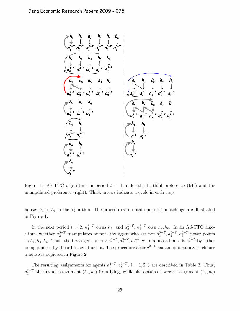
Figure 1: AS-TTC algorithms in period t = 1 under the truthful preference (left) and the
manipulated preference (right). Thick arrows indicate a cycle in each step.
houses ℎ1 to ℎ6 in the algorithm. The procedures to obtain period 1 matchings are illustrated
in Figure 1.
In the next period t = 2, a3−T1 owns ℎ4, and a3−T2 , a3−T3 own ℎ2, ℎ6. In an AS-TTC algo-
rithm, whether a3−T2 manipulates or not, any agent who are not a3−T1 , a3−T2 , a3−T3 never points
to ℎ1, ℎ2, ℎ6. Thus, the first agent among a3−T1 , a3−T2 , a3−T3 who points a house is a3−T1 by either
being pointed by the other agent or not. The procedure after a3−T1 has an opportunity to choose
a house is depicted in Figure 2.
The resulting assignments for agents a2−Ti , a3−Ti , i = 1, 2, 3 are described in Table 2. Thus,
a3−T2 obtains an assignment (ℎ6, ℎ1) from lying, while she obtains a worse assignment (ℎ2, ℎ2)
25
Jena Economic Research Papers 2009 - 075
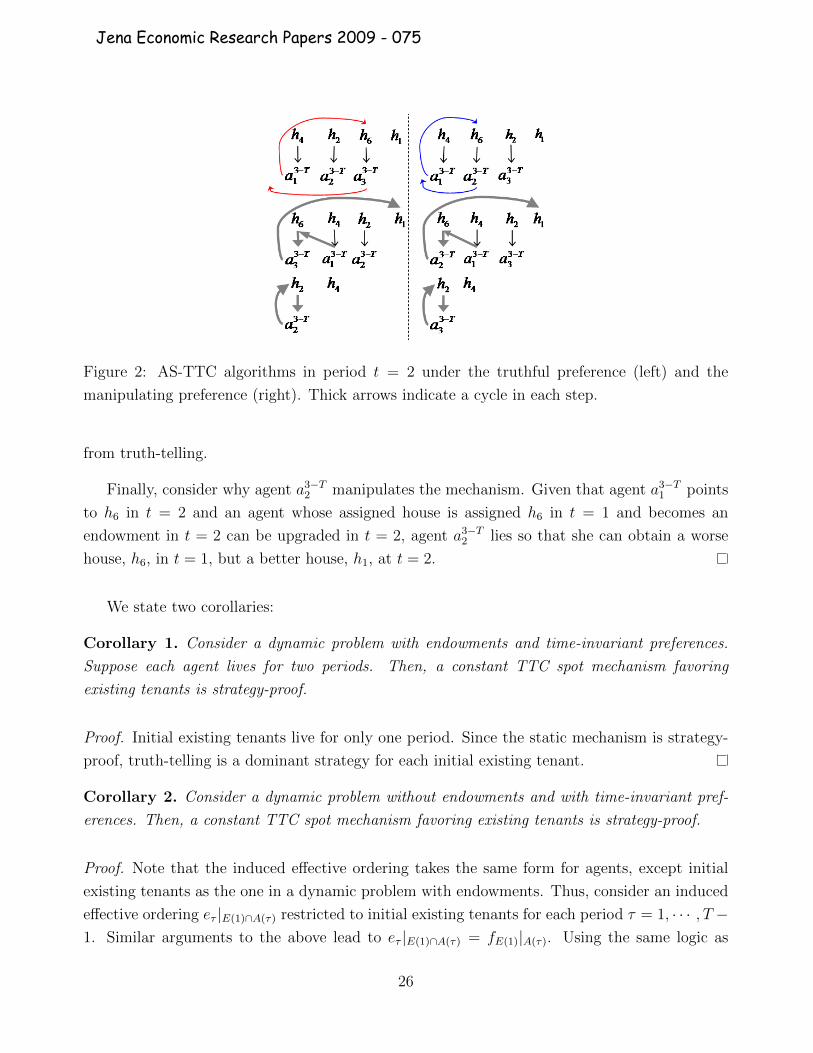
Figure 2: AS-TTC algorithms in period t = 2 under the truthful preference (left) and the
manipulating preference (right). Thick arrows indicate a cycle in each step.
from truth-telling.
Finally, consider why agent a3−T2 manipulates the mechanism. Given that agent a3−T1 points
to ℎ6 in t = 2 and an agent whose assigned house is assigned ℎ6 in t = 1 and becomes an
endowment in t = 2 can be upgraded in t = 2, agent a3−T2 lies so that she can obtain a worse
house, ℎ6, in t = 1, but a better house, ℎ1, at t = 2.
We state two corollaries:
Corollary 1. Consider a dynamic problem with endowments and time-invariant preferences.
Suppose each agent lives for two periods. Then, a constant TTC spot mechanism favoring
existing tenants is strategy-proof.
Proof. Initial existing tenants live for only one period. Since the static mechanism is strategy-
proof, truth-telling is a dominant strategy for each initial existing tenant.
Corollary 2. Consider a dynamic problem without endowments and with time-invariant pref-
erences. Then, a constant TTC spot mechanism favoring existing tenants is strategy-proof.
Proof. Note that the induced effective ordering takes the same form for agents, except initial
existing tenants as the one in a dynamic problem with endowments. Thus, consider an induced
effective ordering e� ∣E(1)∩A(�) restricted to initial existing tenants for each period � = 1, ⋅ ⋅ ⋅ , T −1. Similar arguments to the above lead to e� ∣E(1)∩A(�) = fE(1)∣A(�). Using the same logic as
26
Jena Economic Research Papers 2009 - 075

Theorem 5, we can conclude that the history-independent strategy of true period preferences is
weakly better off than any other history-independent strategy for each initial existing tenant.
5.3 How can a TTC spot mechanism be manipulated by agents who
are not initial existing tenants?
Remember that an SD spot mechanism is strategy-proof. This is because, in each period, it
ignores the past assignment. On the other hand, a TTC spot mechanism guarantees each agent
a house that is at least weakly better than the previously assigned house. This opens up the
possibility of manipulation in which an agent obtains a worse house than she can obtain in
truth-telling, expecting her to be upgraded in an ordering by being pointed out by some other
agent in the next period. As we saw, a constant TTC spot mechanism favoring existing tenants
effectively excludes such a possibility. However, this is not the case if it favors newcomers.
Theorem 6. Consider a dynamic problem with time-invariant preferences either with endow-
ments or without endowments. Suppose there are at least two newcomers in each period. Then,
a TTC spot mechanism favoring newcomers is not strategy-proof among all agents except initial
existing tenants.
Proof. Suppose there are at least two newcomers in each period t ≥ 2 − T . Agents live for
T periods. Pick two newcomers at1 and at2 in each period. Fix a sequence of period orderings
that favors newcomers. Without loss of generality, at1 has higher order than at2 in each period
t. Period preferences Rati(t) (t = 2− T, 3− T, 2, 3; i = 1, 2) of each agent ati satisfy the table on
the left hand side (from best to worst):
a2−T1 a2−T2 a3−T1 a3−T2 a21 a22 a31 a32ℎ2 ℎ3 ℎ1 ℎ4 ℎ1 ℎ1 ℎ2 ℎ4
ℎ3 ℎ2
ℎ2
a21ℎ1
ℎ2
ℎ3
For the other agents, houses ℎ1 to ℎ4 are less preferred to any other house. Moreover, agent a21’s
preference satisfies
(ℎ2, ℎ1, �4a21
)Pa21(ℎ3, ℎ3, �4a21
),
where �4a21
is any assignment of agent a21 from period 4 on. Unspecified preferences are assumed
to be arbitrary.
27
Jena Economic Research Papers 2009 - 075

Endowments are indicated by the parentheses in the first column on the table below. If
T = 2, agents a3−T1 and a3−T2 are not initial existing tenants but newcomers in period 1. However,
the allocations to be calculated will not be affected, even for the case without endowments,
because of preferences.
In each period, we concentrate on a static problem consisting of agents a2−Ti , a3−Ti , a2i , a3i ,
i = 1, 2, since houses ℎ1 to ℎ4 are less preferred to any other house for each of the other agents.
We will see that agent a21 manipulates the mechanism by reporting the preference described
on the right hand side of the above table.
t = 1 t = 2 t = 3 ⋅ ⋅ ⋅a2−T1 (ℎ2) ℎ2
a2−T2 (ℎ3) ℎ3
a3−T1 (ℎ1) ℎ1 ℎ1
a3−T2 (ℎ4) ℎ4 ℎ4...
...
a21 h3 h3 ⋅ ⋅ ⋅a22 ℎ2 ℎ1 ⋅ ⋅ ⋅a31 ℎ2 ⋅ ⋅ ⋅a32 ℎ4 ⋅ ⋅ ⋅...
. . .
t = 1 t = 2 t = 3 ⋅ ⋅ ⋅a2−T1 (ℎ2) ℎ2
a2−T2 (ℎ3) ℎ3
a3−T1 (ℎ1) ℎ1 ℎ1
a3−T2 (ℎ4) ℎ4 ℎ4...
...
a21 h2 h1 ⋅ ⋅ ⋅a22 ℎ3 ℎ3 ⋅ ⋅ ⋅a31 ℎ2 ⋅ ⋅ ⋅a32 ℎ4 ⋅ ⋅ ⋅...
. . .
The left hand side shows an allocation by the TTC spot mechanism when agent a21 reveals her
true preference, while the right hand side shows an allocation by the TTC spot mechanism
when a21 lies. Note that, whether a21 has higher order than a22 in the period 3 ordering or not,
the above assignments are not affected. The procedures to obtain each allocation for period 3
static markets are illustrated in Figure 3 in the case that a21 has higher order than a22 in the
period 3 ordering.
Thus, a21 obtains an assignment (ℎ2, ℎ1, ℎ1, ⋅ ⋅ ⋅ , ℎ1) from lying, while she obtains a worse
assignment (ℎ3, ℎ3, �4a21
) from truth-telling, where �4a21
is some assignment of a21 from period 4 on.
Consider why agent a21 manipulates the mechanism. Given that newcomer a31 points to ℎ2
in t = 3, and an agent whose assigned house is assigned ℎ2 in t = 2 and becomes an endowment
in t = 3 can be upgraded in t = 3, agent a21 lies so that she can obtain a worse ℎ2 in t = 2, but
a better house ℎ1 in t = 3.
28
Jena Economic Research Papers 2009 - 075
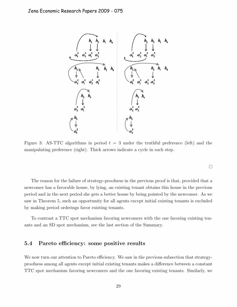
Figure 3: AS-TTC algorithms in period t = 3 under the truthful preference (left) and the
manipulating preference (right). Thick arrows indicate a cycle in each step.
The reason for the failure of strategy-proofness in the previous proof is that, provided that a
newcomer has a favorable house, by lying, an existing tenant obtains this house in the previous
period and in the next period she gets a better house by being pointed by the newcomer. As we
saw in Theorem 5, such an opportunity for all agents except initial existing tenants is excluded
by making period orderings favor existing tenants.
To contrast a TTC spot mechanism favoring newcomers with the one favoring existing ten-
ants and an SD spot mechanism, see the last section of the Summary.
5.4 Pareto efficiency: some positive results
We now turn our attention to Pareto efficiency. We saw in the previous subsection that strategy-
proofness among all agents except initial existing tenants makes a difference between a constant
TTC spot mechanism favoring newcomers and the one favoring existing tenants. Similarly, we
29
Jena Economic Research Papers 2009 - 075

introduce a weaker notion for Pareto efficiency.
Definition 8. A matching plan � Pareto dominates another matching plan � among all
agents except initial existing tenants if
1. {�a(t) : a ∈ A ∖ E(1)} = {�a(t) : a ∈ A ∖ E(1)} for each t ≥ 1, and
2. ∀a ∈ A ∖ E(1), �Ra � and ∃a ∈ A ∖ E(1), �Pa �.
Moreover, a matching plan is Pareto efficient among all agents except initial existing
tenants if it is not Pareto dominated by any other matching plan among all agents except
initial existing tenants.
As with strategy-proofness, a constant TTC spot mechanism favoring existing tenants is
Pareto efficient among all agents except initial existing tenants, but not Pareto efficient.
Theorem 7. Consider a dynamic problem with endowments and time-invariant preferences.
Then, a constant TTC spot mechanism favoring existing tenants is Pareto efficient among all
agents except initial existing tenants, but not Pareto efficient, provided there are at least two
newcomers in each period who live for at least three periods.
Proof. For the first part, let � = {�(t)}∞t=1 be a matching plan generated by a constant TTC
spot mechanism favoring existing tenants for some arbitrary preference profile, R. Let {et}∞t=1 be
a corresponding sequence of effective orderings. To find a contradiction, suppose some matching
plan, �, Pareto dominates � among all agents except initial existing tenants. Then,
∀a ∈ A ∖ E(1), �Ra � and ∃a ∈ A ∖ E(1), �Pa �.
Since A ∖E(1) ≡ ∪∞t=1N(t), take the smallest � ≥ 1 such that ∃a ∈ N(�), �Pa �. It follows from
strict preferences that
∀t ≤ � − 1,∀a ∈ N(t), �a = �a. (4)
In addition, take an agent b ∈ N(�) who has the highest order among agents in {a ∈ N(�) :
�Pa �}. Then, it follows from strict preferences that
∀a ∈ N(�) who has a higher order than b does, �a = �a. (5)
Now, it is sufficient to show that ∀t = �, ⋅ ⋅ ⋅ , � + T − 1, �(t)Rb(t)�(t), since this leads to a
contradiction, namely, that �Rb � and �Pb �. For each t = �, ⋅ ⋅ ⋅ , � + T − 1, it follows from (4)
30
Jena Economic Research Papers 2009 - 075

and (5) that in the effective ordering et, each agent, a, ordered before agent b has �a(t) = �a(t).
Thus, the AS-TTC algorithm implies that there is no room for agent b to be strictly better off
than �b(t). Hence, �(t)Rb(t)�(t).
For the second part, suppose there are at least two newcomers in each period who live for
at least three periods, T . Fix a constant sequence, {fA(t)}∞t=1, of period orderings that favors
existing tenants. Pick initial existing tenants a2−T1 , a2−T2 , a3−T1 , and a3−T2 such that
fA(1)∣{a2−T1 ,a2−T2 ,a3−T1 ,a3−T2 } = (a2−T1 , a2−T2 , a3−T1 , a3−T2 ), and fA(2)∣{a3−T1 ,a3−T2 } = (a3−T1 , a3−T2 ).
Note that a2−Ti lives only in period 1, and a3−Ti lives only in period 1 and 2, i = 1, 2. Each agent
ati ∕= a2−T2 has an identical preference (from best to worst):
Pati(t) : ℎ1, ℎ2, ℎ3.
Agent a2−T2 ’s top choice is ℎ4. For the other agents, houses ℎ1 to ℎ4 are less preferred to any
other house. Moreover,
(ℎ2, ℎ2)Pa3−T1(ℎ3, ℎ1) and (ℎ3, ℎ1)Pa3−T2
(ℎ2, ℎ2).
Endowments are indicated in the first column on the table below.
The induced TTC spot mechanism produces the following assignments:
t = 1 t = 2 t = 3 ⋅ ⋅ ⋅a2−T1 (ℎ1) ℎ1
a2−T2 (ℎ2) ℎ4
a3−T1 (ℎ3) ℎ3 (ℎ2) ℎ1 (ℎ2)
a3−T2 (ℎ4) ℎ2 (ℎ3) ℎ2 (ℎ1)...
Consider another matching plan in which a3−T1 exchanges the first two periods assignments
(ℎ3, ℎ1) for (ℎ2, ℎ2) with a3−T2 . This exchange is described by houses inside the parentheses
on the above table. This matching plan Pareto dominates the one induced by the TTC spot
mechanism.
We state two corollaries:
31
Jena Economic Research Papers 2009 - 075

Corollary 3. Consider a dynamic problem with endowments and time-invariant preferences.
Suppose each agent lives for two periods. Then, a constant TTC spot mechanism favoring
existing tenants is Pareto efficient.
Proof. Pareto efficiency among all agents except initial existing tenants does not consider any
matching that involves an exchange between initial existing tenants and the other agents. How-
ever, when agents live for two periods, initial existing tenants live for only one period. Since
a static AS-TTC spot mechanism is Pareto efficient, any other matching plan involving such a
exchange necessarily hurts the initial existing tenants. Note that this logic does not work for
the case where agents live for at least three periods. Thus, any matching plan induced by a
constant TTC spot mechanism favoring existing tenants is Pareto efficient.
Corollary 4. Consider a dynamic problem without endowments and with time-invariant pref-
erences. Then, a constant TTC spot mechanism favoring existing tenants is Pareto efficient.
Proof. The same argument applies on the induced effective ordering as the one in Corollary
2.
5.5 When is a TTC spot mechanism undesirable?
In an example taken up in Theorem 3 that shows Pareto inefficiency in an SD spot mechanism
favoring newcomers, we demonstrated that an infinite exchange between existing tenants and
newcomers Pareto dominates a matching plan induced by the SD spot mechanism. Looking
at this example closely, we might think that acceptability precludes such an infinite exchange.
Since a TTC spot mechanism satisfies acceptability, one might conjecture that a TTC spot
mechanism favoring newcomers is Pareto efficient. However, this is not the case, as shown in
the following theorem:
Theorem 8. Consider a dynamic problem with time-invariant preferences either with endow-
ments or without endowments. Suppose there are at least two newcomers in each period. Then, a
TTC spot mechanism favoring newcomers is not Pareto efficient among all agents except initial
existing tenants.
Proof. Suppose there are at least two newcomers in each period t ≥ 2 − T . They live for T
periods. Pick two newcomers at1 and at2 in each period. Fix a sequence of period ordering
32
Jena Economic Research Papers 2009 - 075

{fA(t)}∞t=1 that favors newcomers. Without loss of generality, at1 is the first agent in fA(t) in
each period. Note that this sequence may not be constant; e.g., at1 may not be the first in the
subsequent periods. Period preferences satisfy: For each m ≥ 0,
a2Tm+21 a2Tm+2
2 a2Tm+31 a2Tm+3
2 aT (2m+1)+21 a
T (2m+1)+22 a
T (2m+1)+31 a
T (2m+1)+32
ℎ2 ℎ2 ℎ3 ℎ3 ℎ1 ℎ1 ℎ4 ℎ4
ℎ4 ℎ2 ℎ3 ℎ1
ℎ1 ℎ4 ℎ2 ℎ3
ℎ3 ℎ1 ℎ4 ℎ2
a2Tm+22 a2Tm+3
2 aT (2m+1)+22 a
T (2m+1)+32
(ℎ3, �a, ℎ4) (�a, ℎ1, ℎ2) (ℎ4, �a, ℎ3) (�a, ℎ2, ℎ1)
(ℎ1, �a, ℎ1) (�a, ℎ4, ℎ4) (ℎ2, �a, ℎ2) (�a, ℎ3, ℎ3)
where �a ∈ HT−2 is an arbitrary assignment. Moreover,
a2−T1 a2−T2 a3−T1 a3−T2
ℎ1 ℎ2 ℎ3 ℎ4
ℎ ℎ ℎ ℎ
where ℎ is an arbitrary house other than the second row in each column. In the above tables,
each column indicates the corresponding preference where an upper house is strictly preferred
to the lower one. For any other agent not specified above, houses ℎ1 to ℎ4 are less preferred to
any other house.
Endowments are indicated by the parentheses in the first column in Table 3. If T = 2,
agents a3−T1 and a3−T2 are not initial existing tenants but newcomers in period 1. However, the
allocations to be calculated will not be affected, even for the case without endowments, because
of preferences.
In each period, we concentrate on a static problem consisting of agents a2−Ti , a3−Ti , a2Tm+2i ,
a2Tm+3i , a
T (2m+1)+2i , and a
T (2m+1)+3i for i = 1, 2 and m ≥ 0, since houses ℎ1 to ℎ4 are less preferred
to any other house for each of the other agents.
The induced TTC spot mechanism produces the matching plan �, where houses without
parentheses are the assignments, on Table 3. Note that this matching plan is not affected by
whether a sequence of period orderings is constant or not.
33
Jena Economic Research Papers 2009 - 075

Table 3: Matching plans in Theorem 8
1 2 3 ⋅ ⋅ ⋅ T + 1 T + 2 T + 3 ⋅ ⋅ ⋅ 2T + 1 2T + 2 2T + 3 ⋅ ⋅ ⋅a2−T1 (ℎ1) ℎ1
a2−T2 (ℎ2) ℎ2
a3−T1 (ℎ3) ℎ3 ℎ3
a3−T2 (ℎ4) ℎ4 ℎ4...
...
a21 ℎ2 ℎ2 ⋅ ⋅ ⋅ ℎ2
a22 ℎ1 ℎ1 ⋅ ⋅ ⋅ ℎ1(ℎ4)
a31 ℎ3 ⋅ ⋅ ⋅ ℎ3 ℎ3
a32 ℎ4 ⋅ ⋅ ⋅ ℎ4(ℎ1) ℎ4(ℎ2)...
...
aT+21 ℎ1 ℎ1 ⋅ ⋅ ⋅ ℎ1
aT+22 ℎ2(ℎ4) ℎ2 ⋅ ⋅ ⋅ ℎ2(ℎ3)
aT+31 ℎ4 ⋅ ⋅ ⋅ ℎ4 ℎ4
aT+32 ℎ3 ⋅ ⋅ ⋅ ℎ3(ℎ2) ℎ3(ℎ1)...
...
a2T+21 ℎ2 ℎ2 ⋅ ⋅ ⋅a2T+22 ℎ1(ℎ3) ℎ1 ⋅ ⋅ ⋅a2T+31 ℎ3 ⋅ ⋅ ⋅a2T+32 ℎ4 ⋅ ⋅ ⋅
......
Consider an infinite exchange depicted by houses inside the parentheses in Table 3. Clearly,
the resulting allocation Pareto dominates the induced matching plan � among all agents except
initial existing tenants.
See the last section of the Summary to contrast a TTC spot mechanism favoring newcomers
with the one favoring existing tenants and an SD spot mechanism.
34
Jena Economic Research Papers 2009 - 075
6 Serial Dictatorship (SD) Futures Mechanisms
In this section, we consider a dynamic problem without endowments and propose a simple
futures mechanism termed serial dictatorship (SD) futures mechanism. Fix a sequence
(fA(1), {fN(t)}t≥2) of an ordering of initial agents and an ordering of newcomers in period t ≥ 2.
For any announced preference profile, R, an SD futures mechanism finds a matching plan by
using the following algorithm.
Period 1: The first agent in fA(1) gets her top assignment (consisting of houses up to the period
when she leaves the market) under her reported preference. The kth agent in fA(1) gets her top
assignment excluding the houses assigned to all agents before her under her reported preference.
This produces the current matching and the future assignment for agents in A(1).
Period t: Given the assignment determined in past periods, each of the existing tenant is assigned
a house according to her assignment as previously determined. The first newcomer in fN(t) gets
her top assignment excluding the houses assigned to the existing tenants under her reported
preference. A kth newcomer in fN(t) gets her top assignment excluding the houses assigned to
all existing tenants and all newcomers before this agent under her reported preference. The
procedure for newcomers generates the current matching and the future assignment for agents
in A(t).
As such, we have the following.
Theorem 9. In a dynamic problem without endowments, an SD futures mechanism is strategy-
proof and Pareto efficient, but not acceptable under the same assumptions as Impossibility The-
orem 1.
Proof. First, we show strategy-proofness. In period 1, the first agent in fA(1) cannot do better by
reporting any other preference, since she already receives her top assignment under her reported
preference. The kth agent in fA(1) cannot do better than reporting her true preference, since
the house distributed until the kth agent is independent of her preference and receives her top
assignment among the remaining houses. The argument for any other period is similar.
Next, we show Pareto efficiency. To find a contradiction, suppose for some preference profile,
R ∈ ℛ, a matching plan Π(R) given by an SD futures mechanism is not Pareto efficient.
For notational simplicity, let � := Π(R). Then, there exists a matching plan, �, that Pareto
dominates � in R. Thus, ∀a ∈ A, �aRa �a and ∃b ∈ A such that �bPb �b. Since A ≡ A(1) ∪(∪t≥2N(t)), agent b is either in A(1) or in N(t) for some t ≥ 2. Suppose ∀a ∈ A(1) �aRa�a.
35
Jena Economic Research Papers 2009 - 075

Otherwise, the proof is similar to the following and is therefore omitted. Take the smallest t ≥ 2
such that ∃b ∈ N( t ) with �b Pb �b. It follows from strict preferences that ∀a ∈ A(1), �a = �a
and ∀t with 2 ≤ t ≤ t− 1, ∀a ∈ N(t), �a = �a. Consider an agent b ∈ N(t) who has the highest
order in fN(t) such that �bPb�b. Then, it follows from strict preferences that for each agent a
who has higher order than b, �a = �a. Thus, in the SD futures mechanism, when it is agent b’s
turn to choose, two assignments, �b and �b, are still available. Thus, since agent b chooses �b in
the SD futures mechanism, �bRb�b. This is a contradiction.
Since the SD futures mechanism is proved to be Pareto efficient, it follows from Impossibility
Theorem 1 that it is not acceptable.
7 Summary
We summarize some of our results in the tables below.
Table 4: Properties of dynamic mechanisms under “general” preferences
AC SP PE
General SD spot mechanism ✓
Constant SD spot mechanism favoring existing tenants ✓ ✓
SD spot mechanism favoring newcomers ✓
TTC spot mechanism ✓
SD futures mechanism ✓ ✓
Note: AC stands for acceptability, SP stands for strategy-proofness, and PE stands for Pareto efficiency.
The mark “✓” in a cell indicates that a corresponding dynamic mechanism in the first column satisfies the
corresponding properties in the first row. On the other hand, a blank cell indicates that the dynamic mechanism
does not satisfy the property. Moreover, ✓∗ indicates that the spot mechanism is acceptable for a problem
without endowments (See Proposition 2 in the Appendix). ✓∗∗ shows that it is SP (PE) for a problem without
endowments and SP (PE) among all agents except initial existing tenants for a problem with endowments.
These results verify the desirableness of seniority-based mechanisms.
36
Jena Economic Research Papers 2009 - 075

Table 5: Properties of dynamic mechanisms under “time-invariant” preferences
AC SP PE
General SD spot mechanism ✓
Constant SD spot mechanism favoring existing tenants ✓∗ ✓ ✓
SD spot mechanism favoring newcomers ✓
General TTC spot mechanism ✓
Constant TTC spot mechanism favoring existing tenants ✓ ✓∗∗ ✓∗∗
TTC spot mechanism favoring newcomers ✓
SD futures mechanism ✓ ✓
Appendix
Proposition 2. Consider a dynamic problem with time-invariant preferences and without en-
dowments. A constant SD spot mechanism favoring existing tenants is acceptable.
Proof. Suppose that an agent, a, obtains some house ℎ at some period t. Since agents before
agent a do not prefer the house ℎ in period t, in the next period, it follows from time-invariant
preferences that agents before agent a do not obtain this house, and thus agent a has an option
of getting house ℎ or one of the remaining houses. Hence, agent a is weakly better off as time
goes on.
References
[1] Abdulkadiroglu, Atila, and Simon Loertscher (2007) “Dynamic House Allocations.” Working
papar.
[2] Abdulkadiroglu, Atila, and Tayfun Sonmez (1998) “Random Serial Dictatorship and the
Core from Random Endowments in House Allocation Problems.” Econometrica, 66, 689-
701.
[3] Abdulkadiroglu, Atila, and Tayfun Sonmez (1999) “House Allocation with Existing Ten-
ants.” Journal of Economic Theory, 88, 233-260.
37
Jena Economic Research Papers 2009 - 075

[4] Abdulkadiroglu, Atila and Tayfun Sonmez (2003) “School Choice: A Mechanism Design
Approach.” American Economic Review, 93, 729-747.
[5] Athey, Susan, and Ilya Segal (2007) “An Efficient Dynamic Mechanism.” Working paper.
[6] Bloch, Francis, and David Cantala (2008) “Markovian Assignment Rules.” Woring paper.
[7] Chen, Yan and and Tayfun Sonmez (2002) “Improving Efficiency of On-Campus Housing:
An Experimental Study.” American Economic Review, 92, 1669-1686.
[8] Frederick, Shane, George Loewenstein, and Ted O’Donoghue (2002) “Time Discounting and
Time Preference: A Critical Review.” Journal of Economic Literature, Vol.XL(June 2002),
351-401.
[9] Gershkov, Alex, and Benny Moldovanu (2009) “Dynamic Revenue Maximization with Het-
erogeneous Objects: A Mechanism Design Approach.” American Economic Journal: Mi-
croeconomics, forthcoming.
[10] Guillen, Pablo, and Onur Kesten (2008) “On-Campus Housing: Theory vs. Experiments.”
Woring paper.
[11] Hylland, Aanund, and Richard Zeckhauser (1979) “The Efficient Allocation of Individuals
to Positions.” Journal of Political Economy, 87, 293-314.
[12] Konishi, Hideo, Thomas Quint, and Jun Wako (2001) “On the Shapley-Scarf Economy:
The Case of Multiple Types of Indivisible Goods.” Journal of Mathematical Economics, 35,
1-15.
[13] Ljungqvist, Lars, and Thomas J. Sargent (2004) Recursive Macroeconomic Theory, 2nd
edition, MIT press.
[14] Roth, Alvin E., Tayfun Sonmez, and M. Utku Unver (2004) “Kidney Exchange.” Quarterly
Journal of Economics, 119, 457-488.
[15] Samuelson, Paul A. (1958) “An Exact Consumption-Loan Model of Interest with or without
the Social Contrivance of Money.” Journal of Political Economy, 66, 467-482.
[16] Shapley, Lloyd and Herbert Scarf (1974) “On Cores and Indivisibility.” Journal of Mathe-
matical Economics. 1, 23-28.
[17] Shell, Karl (1971) “Notes on the Economics of Infinity.” Journal of Political Economy, 79,
1002-1011.
38
Jena Economic Research Papers 2009 - 075

[18] Sonmez, Tayfun, and M. Utku Unver (2005) “House Allocation with Existing Tenants: An
Equivalence.” Games and Economic Behavior, 52, 153-185.
[19] Sonmez, Tayfun, and M. Utku Unver (2008) “Matching, Allocation, and Exchange of Dis-
crete Resources.” Jess Bennhabib, Alberto Bisin, and Matthew Jackson (eds.) Handbook of
Social Economics, Elseview, forthcoming.
[20] Svensson, Lars-Gunnar (1994) “Queue Allocation of Indivisible Goods,” Social Choice and
Welfare, 11, 323-330.
[21] Unver, M. Utku (2009) “Dynamic Kidney Exchange.” Forthcoming in Review of Economic
Studies.
39
Jena Economic Research Papers 2009 - 075