
HoursandEmploymentOvertheBusinessCycle: …njtraum/CFT_Hours.pdf · · 2017-11-09the...
42
Hours and Employment Over the Business Cycle: A Bayesian Approach * Matteo Cacciatore † HEC Montr´ eal and NBER Giuseppe Fiori ‡ North Carolina State University Nora Traum § North Carolina State University November 8, 2017 Abstract We show that an estimated business cycle model with search-and-matching frictions and a neoclassical hours-supply decision cannot account for the cyclical behavior of U.S. hours and employment and their comovement with macroeconomic variables. A parsimonious set of fea- tures reconciles the model with the data: non-separable preferences with parametrized wealth effects and costly hours adjustment. The model, estimated with Bayesian methods, offers a structural explanation for the observation that in post-war U.S. recoveries, the covariance be- tween the labor margins is either positive or negative. The contribution of hours per worker to total hours is quantitatively significant, with a notable component stemming from its indirect effect on employment adjustment. JEL Codes : C11, E24, E32. Keywords : Bayesian Estimation, Business Cycles, Employment, Hours. * First Version: February 15, 2016. For helpful comments, we thank Alejandro Justiniano, Evi Pappa, Federico Ravenna, Morten Ravn, Luca Sala, as well as seminar and conference participants at the 2016 International Asso- ciation for Applied Econometrics Conference, the 2017 ICMAIF Conference, the EEA-ESEM 2016 Conference, the New York Fed “New Developments in the Macroeconomics of Labor Markets” Conference, the Bank of Canada, the Cleveland Federal Reserve, the Danmarks Nationalbank, the Kiel Institute for the World Economy, the Magyar Nemzeti Bank, and the Saint Louis Federal Reserve. † HEC Montr´ eal, Institute of Applied Economics, 3000, chemin de la Cˆ ote-Sainte-Catherine, Montr´ eal (Qu´ ebec). E-mail: [email protected]. URL: http://www.hec.ca/en/profs/matteo.cacciatore.html. ‡ North Carolina State University, Department of Economics, 2801 Founders Drive, 4150 Nelson Hall, Box 8110, 27695-8110 - Raleigh, NC, USA. E-mail: gfi[email protected]. URL: http://www.giuseppefiori.net. § North Carolina State University, Department of Economics, 2801 Founders Drive, 4150 Nelson Hall, Box 8110, 27695-8110 - Raleigh, NC, USA. E-mail: [email protected]. URL: http://www4.ncsu.edu/ ~ njtraum/.
Transcript of HoursandEmploymentOvertheBusinessCycle: …njtraum/CFT_Hours.pdf · · 2017-11-09the...

Hours and Employment Over the Business Cycle: A Bayesian
Approach∗
Matteo Cacciatore†
HEC Montreal and NBER
Giuseppe Fiori‡
North Carolina State University
Nora Traum§
North Carolina State University
November 8, 2017
Abstract
We show that an estimated business cycle model with search-and-matching frictions and a
neoclassical hours-supply decision cannot account for the cyclical behavior of U.S. hours and
employment and their comovement with macroeconomic variables. A parsimonious set of fea-
tures reconciles the model with the data: non-separable preferences with parametrized wealth
effects and costly hours adjustment. The model, estimated with Bayesian methods, offers a
structural explanation for the observation that in post-war U.S. recoveries, the covariance be-
tween the labor margins is either positive or negative. The contribution of hours per worker to
total hours is quantitatively significant, with a notable component stemming from its indirect
effect on employment adjustment.
JEL Codes : C11, E24, E32.
Keywords : Bayesian Estimation, Business Cycles, Employment, Hours.
∗First Version: February 15, 2016. For helpful comments, we thank Alejandro Justiniano, Evi Pappa, FedericoRavenna, Morten Ravn, Luca Sala, as well as seminar and conference participants at the 2016 International Asso-ciation for Applied Econometrics Conference, the 2017 ICMAIF Conference, the EEA-ESEM 2016 Conference, theNew York Fed “New Developments in the Macroeconomics of Labor Markets” Conference, the Bank of Canada,the Cleveland Federal Reserve, the Danmarks Nationalbank, the Kiel Institute for the World Economy, the MagyarNemzeti Bank, and the Saint Louis Federal Reserve.
†HEC Montreal, Institute of Applied Economics, 3000, chemin de la Cote-Sainte-Catherine, Montreal (Quebec).E-mail: [email protected]. URL: http://www.hec.ca/en/profs/matteo.cacciatore.html.
‡North Carolina State University, Department of Economics, 2801 Founders Drive, 4150 Nelson Hall, Box 8110,27695-8110 - Raleigh, NC, USA. E-mail: [email protected]. URL: http://www.giuseppefiori.net.
§North Carolina State University, Department of Economics, 2801 Founders Drive, 4150 Nelson Hall, Box 8110,27695-8110 - Raleigh, NC, USA. E-mail: [email protected]. URL: http://www4.ncsu.edu/~njtraum/.

1 Introduction
A vast literature addresses the cyclical behavior of the labor market in the context of the Mortensen-
Pissarides search and matching model (Mortensen and Pissarides, 1994, and Pissarides, 2000), ar-
guably the benchmark theory of equilibrium unemployment today.1 Nevertheless, the majority of
this literature ignores the distinction between changes in average hours per worker (the intensive
margin) versus movements in and out of employment (the extensive margin).2 Omitting the com-
positional adjustment of total hours worked is not without loss of generality. Changes in hours per
worker are about as large as changes in employment in many OECD countries (Ohanian and Raffo,
2012). In the U.S., the volatility of the intensive margin accounts for approximately one-third of
the unconditional variability of aggregate hours. Moreover, in specific U.S. business cycle episodes,
the two margins covary either positively or negatively, and their relative contribution to aggregate
fluctuations is time-varying.3
In this paper, we take up the challenge of accounting for and explaining the cyclical behavior
of the margins of labor adjustment and their comovement with the rest of the economy. These
relations are central for policy prescriptions and welfare analysis from quantitative business-cycle
models, as labor market responses shape the dynamics of key policy variables like the output
gap. We first determine under which conditions a business cycle model that features search-and-
matching frictions can account for macro data that include both margins of labor adjustment.
We then provide a structural assessment of the contribution of the intensive margin to aggregate
fluctuations, shedding new light on the sources of labor market dynamics.
Our baseline specification utilizes a state-of-the-art business cycle model that successfully ac-
counts for key macroeconomic time-series, as shown in Christiano et al. (2005), Smets and Wouters
(2007), and Justiniano et al. (2010).4 We embed a labor market structure that follows the conven-
tional approach in search and matching models that include the intensive margin—see Andolfatto
(1996), Arseneau and Chugh (2008), Christiano et al. (2011), Ravenna and Walsh (2012), and
Trigari (2009), to name a few.5 Firms adjust labor inputs either by posting vacancies or changing
1See, among others, Andolfatto (1996), den Haan et al. (2000), Gertler and Trigari (2009), and Shimer (2005).2Some early contributions, including Cho and Cooley (1994), Kydland and Prescott (1991), and Hansen and
Sargent (1988), calibrate models in which the supply of total hours adjust along both the intensive and extensivemargins, but abstract from search and matching frictions.
3Section 2 discusses the data and robustness of these computations. In addition, we document that the positivecovariance between hours per worker and employment is a significant contributor to total hours variation.
4The model features habit formation, investment adjustment costs, variable capital utilization, and nominal priceand wage rigidities.
5These studies do not assess the ability of the search and matching model to account for the cyclicality of the
1

the number of hours per worker. Households face a standard neoclassical hours-supply decision,
which also is consistent with the business cycle literature. In equilibrium, hours per worker adjust
to equate the marginal rate of substitution between hours and consumption to the value of the
marginal product of hours. The widespread preference for this setup stems from its invariance to
the Barro (1977) critique, since wages do not have a direct impact on on-going worker-employer
relations (and thus on the adjustment of hours per worker).6
We estimate the model using Bayesian inference with U.S. data.7 Our full information approach
provides an ideal laboratory to study the empirical performance of the model, since it allows us
to evaluate the model fit relative to a large set of macro moments, beyond pure labor market
outcomes. Moreover, it allows us to encompass most of the views on the sources of business cycles
found in the literature, giving disturbances other than the neutral technology shock a fair chance
of accounting for labor market adjustments.
Our analysis yields three main results. First, the baseline model cannot account for the cycli-
cality of the margins of labor adjustment. In particular, the model cannot reproduce the positive
unconditional covariance between employment and hours per worker, and it generates counterfac-
tual volatilities for both labor margins. The model also cannot account for the covariance between
both labor margins and macroeconomic times series; namely it generates counterfactually low (high)
comovement of hours per worker (employment) with aggregate output and consumption. The main
issue is that the model implies a countercyclical behavior of hours per worker conditional on both
technology and demand shocks, a result contrary to existing VAR evidence—see for instance, Ravn
and Simonelli (2007). Moreover, the intensive margin’s relative volatility is counterfactually high
in the presence of hours supply shocks.
Our second contribution is to reconcile the model with the data. Two candidate explanations
for the counterfactual labor market dynamics are the strength of short-run wealth effects on la-
bor supply, which affects the response of hours per worker to TFP and demand shocks, and the
asymmetric costs of adjusting the two labor margins, since posting vacancies is costly, while hours
per worker are frictionless. For these reasons, we introduce additional flexibility in the model by
labor margins, nor do they address the contribution of fluctuations in hours per worker to labor market and aggregatedynamics.
6Two alternative determinations of hours per worker occasionally considered in the literature are right-to-manageand joint Nash bargaining over wages and hours per worker—Nash bargaining implies that hours per worker no longersatisfy the standard neoclassical condition in the presence of wage rigidities. Both setups are not immune to Barro’scritique. We explore the fit of these alternative setups, finding that the performance of both models is inferior to thebaseline specification.
7To avoid the effective lower bound on monetary policy, we exclude the Great Recession for estimation.
2

including two ancillary features: non-separable preferences that feature parametrized wealth effects
on labor supply as in Jaimovich and Rebelo (2009) and costly hours’ adjustment.8,9 We re-estimate
the model and find strong support in favor of weak short-run wealth effects and positive hours
adjustment costs. Intuitively, weakening the wealth effect eliminates the negative comovement be-
tween hours per worker and employment and increases the comovement of hours per worker with
both output and investment. The presence of costly hours’ adjustment prevents excessive variabil-
ity in hours per worker, the second key dimension for reproducing the cyclical behavior of both
margins of labor adjustment.
Finally, we examine the behavior of hours and employment in post-WWII U.S. recessions and
recoveries, as there has been revitalized interest in labor-market dynamics in the wake of the Great
Recession. The estimated model offers a structural interpretation for the observed time-varying
comovement between hours per worker and employment in these periods. Hours and employment
comove positively in response to demand and supply shocks, and comove negatively in response to
labor-market shocks—shocks that affect the rigidity of real wages and hours supply. Moreover, a
model counterfactual shows that adjustment in hours per worker had sizable effects on the recovery
of total hours (up to 3.5 percentage points). A notable component stems from the indirect effect of
hours per worker on employment (beyond the direct effect of hours per worker on total hours): the
intensive-margin adjustment increases employment losses during recessions and delays employment
recoveries.
To understand the indirect effect of hours per worker on employment, we examine the aggregate
dynamics when hours per worker are constant. With the intensive margin fixed, the expected
present discounted value of new matches varies less in response to shocks that induce positive
comovement between the margins of labor. Accordingly, firms adjust effective capital more than
employment, holding all else constant. Lack of adjustment in the intensive margin also implies that
firms can no longer substitute away from the relatively cheaper labor input in response to shocks
that induce a negative comovement between the margins of labor. As a result, both effects imply
that fluctuations in hours per worker increase the response of employment to aggregate shocks.
8The preference specification in Jaimovich and Rebelo (2009) allows us to study the limiting case of no wealtheffects considered by Greenwood et al. (1988), while preserving the existence of balanced growth in the model. Imbenset al. (1999) provide microeconomic evidence of weak short-run wealth effects.
9In the data, hours adjustment is constrained both by the regulation of working time, as well as technologicalfrictions. For instance, the “Wages and the Fair Labor Standards Act” establishes that covered nonexempt employeesin both private and public sectors must receive overtime pay at one-half times the regular rate for hours over 40 perweek. Moreover, the incidence of flexible work hours varies by occupation (Beers, 2000); it is lower for jobs that dictateset intervals for work (e.g., nurses, firefighters, pilots) and most common among workers in executive, administrative,sales and managerial occupations. Other technological constraints include set-up costs and coordination issues.
3

We consider several robustness exercises that support our results. Issues with the baseline model
hold regardless of the number of labor-market observables included in the estimation—either total
hours alone or hours and employment together—and the shocks that affect labor adjustment.10
Issues hold also regardless of the data-measure for labor-market variables and wages. In addition,
the counterfactual behavior of the baseline model is not intrinsically linked to a specific value of
the Frisch elasticity of labor supply.11
While we estimate the model on U.S. data, the results of our paper are broader in scope. First,
as documented by Ohanian and Raffo (2012), hours and employment positively comove in several
economies (for instance, in the U.K., Canada, and Japan), suggesting that the inability of the
baseline model to account for the margins of labor adjustment is not limited to the U.S. economy.
Second, parametrized wealth effects and costly hours’ adjustment introduce enough flexibility to
allow the model to match a broad array of empirical regularities about hours per worker and
employment, including potentially negative ones observed in some European economies.
This paper relates to several strands of the literature. First, since Shimer (2005), a large
literature addresses the ability of the search and matching model to replicate the cyclical behavior
of vacancies and employment. While the debate has for the most part focused on calibrated versions
of the search model, a few recent contributions examine the issue in the context of quantitative,
estimated models (Christiano et al., 2016, Gertler et al., 2008, and Justiniano and Michelacci,
2012).12 In contrast, we document the inability of the model to jointly reproduce the cyclical
behavior of hours per worker, employment, and their empirical covariances with macroeconomic
time series.
This paper also relates to the literature addressing the behavior of employment in U.S. cyclical
recoveries. In particular, an active strand of research addresses the so-called “jobless recoveries”
following the past three U.S. recessions (of 1991, 2001, and 2009), where aggregate employment
continued to decline for years following the turning point in aggregate income and output.13 Our
10When we estimate using aggregate hours as the only labor market observable, we either consider a standardbargaining power shock or a shock that affects the hours margin. When we include hours and employment asobservables, we consider simultaneously the bargaining power shock and a hours supply shock.
11While our estimates for this elasticity are aligned with microeconometric evidence, the inability of the model toreproduce the margins of labor adjustment persists even when we calibrate the Frisch elasticity to values used in themacroeconomic literature, as such values counterfactually augment the intensive margin’s variability.
12Christiano et al. (2011) estimate a small-open economy model featuring search and matching frictions and en-dogenous hours per worker. They focus on the role of shocks and frictions for business cycle dynamics, withoutaddressing the model’s capability to capture the margins of labor adjusmtnet. Altug et al. (2011) show that financialfrictions contribute to the dynamics of employment and hours per worker in a small-open economy model calibratedto match features of emerging economies. Balleer et al. (2016) identify, quantify, and interpret the dynamics ofshort-time work (i.e., publicly subsidized work time reductions) in Germany.
13No consensus has yet emerged regarding the source of jobless recoveries. Some attribute the occurrence of this
4

results provide additional insights to the debate by emphasizing the role of hours’ adjustment for
employment dynamics during these episodes.
The rest of the paper is organized as follows. Section 2 reviews the empirical relation of U.S.
hours and employment. Section 3 outlines the model. Section 4 describes the approach for inference
and discusses the cyclical behavior of the margins of labor adjustment in the estimated baseline
model. Section 5 studies the performance of the alternative model featuring parameterized wealth
effects and hours adjustment costs. Section 6 discusses the cyclical behavior of hours per worker
and employment in post-war U.S. recoveries. Section 7 evaluates the robustness of the results to
alternative model specifications. Section 8 concludes.
2 Hours and Employment in the Data
We begin with a review of stylized facts about U.S. hours per worker, employment, and total hours
worked. In contrast to previous work, we use measures of total hours worked and employment
for the entire economy constructed by the BLS from the Current Employment Statistics (CES)
survey.14 Francis and Ramey (2009) show this economy-wide total hours series is less sensitive to
sectoral shifts than nonfarm business sector measures. First, we find the covariance of hours per
worker and total hours can account for up to 30 percent of the unconditional variation in total
hours. Second, hours per worker and employment positively co-move. The positive covariance of
the intensive and extensive margins is a substantial contributor to the variability of total hours
(20 − 30%), on top of the direct share of hours per worker’s variance (10-18%). Third, both the
comovement and the relative contribution of the intensive margin varies in specific business cycle
episodes. We illustrate this by showing time-variation in the intensive margin’s contribution to
recessions and recoveries. We also highlight the robustness of these facts across alternative labor
data sets and discuss their importance for explaining fluctuations in aggregate hours.
We use quarterly data over the period 1965:1-2007:4, which corresponds to the estimation sample
period in section 4.15 Hours per worker is constructed from the total hours and employment series.
phenomenon to fundamental changes in the underlying economic structure (e.g., Schreft et al., 2005 and Groshenand Potter, 2003). Others focus on cyclical explanations, such as the intensive margin of labor adjustment in thewake of a short and shallow recession (Bachmann, 2012). Jaimovich and Siu (2012) show that jobless recoveries inthe aggregate are accounted for by jobless recoveries in the middle-skill occupations that are disappearing becauseof job polarization. Gali et al. (2012) study slower recoveries in an estimated model that abstracts from endogenousfluctuations in hours per worker.
14This data is publicly available from the BLS website at www.bls.gov/lpc/special_requests/us_total_hrs_emp.xlsx.To construct a total economy series, the Current Employment Statistics data is supplemented from other sources.See the BLS website for details.
15Results are similar using a longer data sample from 1965:1-2014:4, as documented in appendix A.
5

Total hours and employment are divided by the civilian non-institutional population to express
in per capita terms. All variables are expressed in logs and multiplied by 100. Over the sample
period, employment exhibits an upward trend while hours per worker exhibits a downward trend.16
We consider several alternative detrending methods. Our preferred method removes a linear trend
from each series, which corresponds to the series used for estimation in section 4. When hours
and employment are linearly detrended, their sum almost perfectly matches the original, demeaned
total hours series (their correlation is over 0.99). Thus, the linear filtering appears to account for
the low-frequency structural features of employment and hours per worker while preserving the
original properties of the total hours series. In addition, we apply a HP filter with smoothing
parameters of 1600 and 105 and a band pass filter as in Christiano and Fitzgerald (2003).
To assess the contribution of the intensive margin to labor adjustment, we consider two standard
decompositions of the variance of total hours. The first decomposition exploits the fact that
var(THt) = cov(THt, ht) + cov(THt, Lt),
where THt is total hours worked, ht is hours per worker, and Lt is employment. Using this decom-
position, we compute the shares of the variance attributed to hours per worker and employment
as
βcov,h ≡cov(THt, ht)
var(THt), βcov,L ≡
cov(THt, Lt)
var(THt).
In addition, we consider the following alternative decomposition:
var(THt) = var(ht) + var(Lt) + 2cov(ht, Lt),
and define the shares of the variance attributed to hours per worker, employment, and the covariance
term respectively as
βh ≡var(ht)
var(THt), βL ≡
var(Lt)
var(THt), βcov ≡
2cov(ht, Lt)
var(THt).
Table 1 displays these variance shares for the alternative detrending methods. While em-
16As shown by Kirkland (2000), the decline in average hours per worker recorded by the CES survey can beattributed to the disproportionate increase of nonsupervisory workers in retail trade and services—the two industrydivisions in the service-producing sector with the lowest average weekly hours—together with the decline in thepercentage of production workers in mining and manufacturing—the two divisions with the highest number of averageweekly hours. See also Wolters (2016) for a discussion of low-frequency movements in hours per worker.
6

ployment accounts for the largest share of variation in total hours, the intensive margin plays a
quantitatively significant role. The first decomposition shows that the covariance between hours
per worker and total hours (βcov,h) accounts for up to one-third of the total variation in THt. The
second decomposition shows that the positive covariance between hours and employment (βcov) ex-
plains approximately one-third of the variability in total hours. Thus, fluctuations in the intensive
margin affect total hours both directly and indirectly through employment.
Table 1: Decomposition of Total Hours and Labor Market Comovement
Filtering(
cov(THt,ht)var(THt)
) (cov(THt,Lt)var(THt)
) (var(ht)
var(THt)
) (var(Lt)var(THt)
) (2cov(ht,Lt)var(THt)
)
Linear 0.33 0.67 0.18 0.51 0.31HP 1600 0.21 0.79 0.10 0.67 0.23HP 105 0.25 0.75 0.10 0.60 0.30BP 0.23 0.77 0.10 0.63 0.27
Appendix A documents the robustness of these results to two alternative data sources. The first
uses labor variables from the Current Population Survey (CPS) which are augmented with armed
forces data to provide an alternative economy-wide measure, as in Ramey (2012). CPS total hours
data exhibit less pronounced low-frequency variation than CES measures, as shown by Frazis and
Stewart (2010). Our results are robust to unfiltered and filtered measures of these variables. In
addition, the results remain when using the labor market variables of Smets and Wouters (2007),
which are widely employed in the DSGE estimation literature. In this case, hours per worker can
contribute approximately 50 percent of the variation in total hours.
While Table 1 documents an unconditional positive correlation between hours per worker and
employment, the comovement varies in specific episodes. To illustrate this, the bottom panel of
figure 1 plots total hours, employment, and hours per worker during five recession-recovery episodes:
1970:1, 1975:1, 1982:4, 1991:1, and 2001:4.17 For reference, the figure displays the first difference
of the natural logarithm of GDP as well (top panel). We display employment and hours per
worker relative to their linear trends. Hours per worker and employment positively co-move in
some recoveries, such as 1982:4, but negatively co-move in other episodes, as in 1991:1. In addition,
hours per worker is quantitatively important for aggregate hours in several recoveries. For instance,
at the 1982:4 trough, the difference in employment and total hours relative to trend was over two
17The literature comparing employment measures in jobless recoveries suggests preference for CES data measuressimilar to those used here. See Bachmann (2012) for a review of the literature.
7

2 4 6 8
−1
0
1
2
1970.4
2 4 6 8
−1
0
1
2
1975.1
2 4 6 8
−1
0
1
2
1982.4
2 4 6 8
−1
0
1
2
1991.1
2 4 6 8
−1
0
1
2
2001.4
GDP Growth
2 4 6 8
−1
0
1
2
3
4
5
1970.4
2 4 6 8−7
−6
−5
−4
−3
−2
−1
1975.1
2 4 6 8−8
−7
−6
−5
−4
−3
−2
1982.4
2 4 6 8
−1
0
1
2
1991.1
Decomposition of Total Hours in U.S. Recoveries
2 4 6 8−1
0
1
2
3
4
2001.4
Total HoursEmploymentHours
Figure 1. U.S. cyclical recoveries. Solid vertical lines indicate the troughs, using the NBER dates. Labordata are measures for the entire economy.
percentage points, whereas four quarters later the gap shrunk to a difference of about one percentage
point (see the bottom row, column three). The closing of the gap was due to hours per worker,
which was rising on average over the period. Likewise, in the recovery of 2001:4, total hours and
hours per worker exhibited a short increase two periods after GDP’s trough, while employment
steadily declined over the whole episode. As shown in Appendix A, the time-varying comovement
in recession-recovery episodes is robust across different detrending methods and alternative data
sources.
In the subsequent sections, we focus on developing a model consistent with these patterns in
the data.
3 The Model
This section outlines a medium-scale, dynamic stochastic general equilibrium model that features
labor-market search and matching frictions. The model shares salient details that many have found
useful for capturing features of the data. These include habit formation, costs of adjusting the flow
of investment, variable capital utilization, and nominal price and wage rigidities.
8

The modeling of the labor market follows closely the existing literature, with two important
generalizations. First, we consider a general class of preferences that allow us to parameterize
the strength of short-run wealth effects on the labor supply. Second, we introduce costly hours
adjustment. The model nests the standard framework analyzed in the literature, absent hours
adjustment costs and with household’s preferences restricted to be additively separable.
Finally, we abstract from monetary frictions that would motivate a demand for currency and
model a cashless economy following Woodford (2003). Below, variables without a time subscript
denote non-stochastic values along the balanced growth path.
Household Preferences
The economy is populated by a representative household with a continuum of members along the
unit interval. In equilibrium, some family members are unemployed, while others are employed.
As is common in the literature, we assume that family members perfectly insure each other against
variation in labor income due to changes in employment status, so that there is no ex post hetero-
geneity across individuals in the household (see Andolfatto, 1996, and Merz, 1995).
Household’s per-period utility depends on current consumption, Ct, lagged consumption Ct−1
(due to the presence of habit formation), and the disutility of hours supplied by employed members:
Ht ≡ ht∫ Lt
0 v (hjt) dj, where Lt denotes the mass of employed workers, hjt denotes hours worked by
the employed member j, and v (·) is a convex function. The term ht denotes an exogenous shock
to the marginal disutility of hours worked, which evolves according to log ht = ρh log ht−1 + εht
with εhtiid∼ N
(0, σ2
h
). The representative household maximizes the expected intertemporal utility
function
Wt ≡ Et
∞∑
s=t
βs−tβs [u (Cs, Cs−1,Ht)] , (1)
where β ∈ (0, 1) is the discount factor and βt denotes an exogenous shock to the discount factor,
which evolves according to log βt = ρβ log βt−1 + εβt with εβtiid∼ N
(0, σ2
β
).
As discussed in the next section, we consider two alternative specifications for u (·): addi-
tively separable preferences (the benchmark in the literature), and non-separable preferences with
parametrized wealth effects.
The consumption basket Ct aggregates differentiated consumption varieties, Cωt, in Dixit-
Stiglitz form: Ct =
[∫ 10 C
(θt−1)/θtωt dω
]θt/(θt−1)
, where θt > 1 is the exogenous elasticity of sub-
stitution across goods. We assume that θt follows the stochastic process log θt = ρθ log θt−1 +
9

(1− ρθ) log θ + εθt, where εθtiid∼ N
(0, σ2
θ
), which, following the literature, we refer to as a price
markup shock. The corresponding price index is given by: Pt =[∫ 1
0 P 1−θωt dω
]1/(1−θ)
, where Pωt is
the price of variety ω.
Production
There are two vertically integrated production sectors. In the upstream sector, perfectly competitive
firms use capital and labor to produce a homogenous intermediate input. In the downstream sector,
monopolistically competitive firms purchase intermediate inputs and produce the differentiated
varieties that are sold to consumers. This production structure is common in the search and
matching literature featuring nominal rigidities and monopolistic competition, as it simplifies the
introduction of labor market frictions in the model; see, for instance, Gertler et al. (2008), Ravenna
and Walsh (2011), and Trigari (2009).
Intermediate Input Producers
There is a unit mass of perfectly competitive intermediate producers. Production requires capital
and labor. Within each firm there is a continuum of jobs; each job is executed by one worker. Cap-
ital is perfectly mobile across firms and jobs and there is a competitive rental market in capital. All
jobs produce with identical exogenous productivity At. We assume that the growth rate of technol-
ogy, gAt ≡ At/At−1, follows the stochastic process: log gAt = ρgA log gAt−1+(1− ρgA) log gA+ εgAt,
where εgAtiid∼ N
(0, σ2
gA
).
A filled job in the representative firm j produces (kjt)a(Athjt
)1−αunits of output, where kjt is
the stock of capital allocated to the job and hjt ≡ hjt
[1− φh
2 (hjt − hj)2]denotes hours per worker
net of a cost of adjustment φh > 0.18 The latter adjustment cost captures various frictions that
constrain the ability of firms to adjust hours per worker—for instance, technological constraints
due to set-up costs and coordination issues. Total producer’s output exhibits constant returns to
scale in total effective hours and capital:
Y Ijt = Kα
jt
(AtLjthjt
)1−α, (2)
where Ljt is the measure of jobs within the firm and Kjt ≡ Ljtkjt.19
18Since all jobs produce with identical aggregate productivity At, all existing matches produce the same amountof output using the same capital and hours inputs. For this reason, we omit a job-specific index.
19This stems from the fact that Y Ijt = Ljt (kjt)
a(
Athjt
)1−α
= Kαjt
(
AtLjthjt
)1−α
.
10
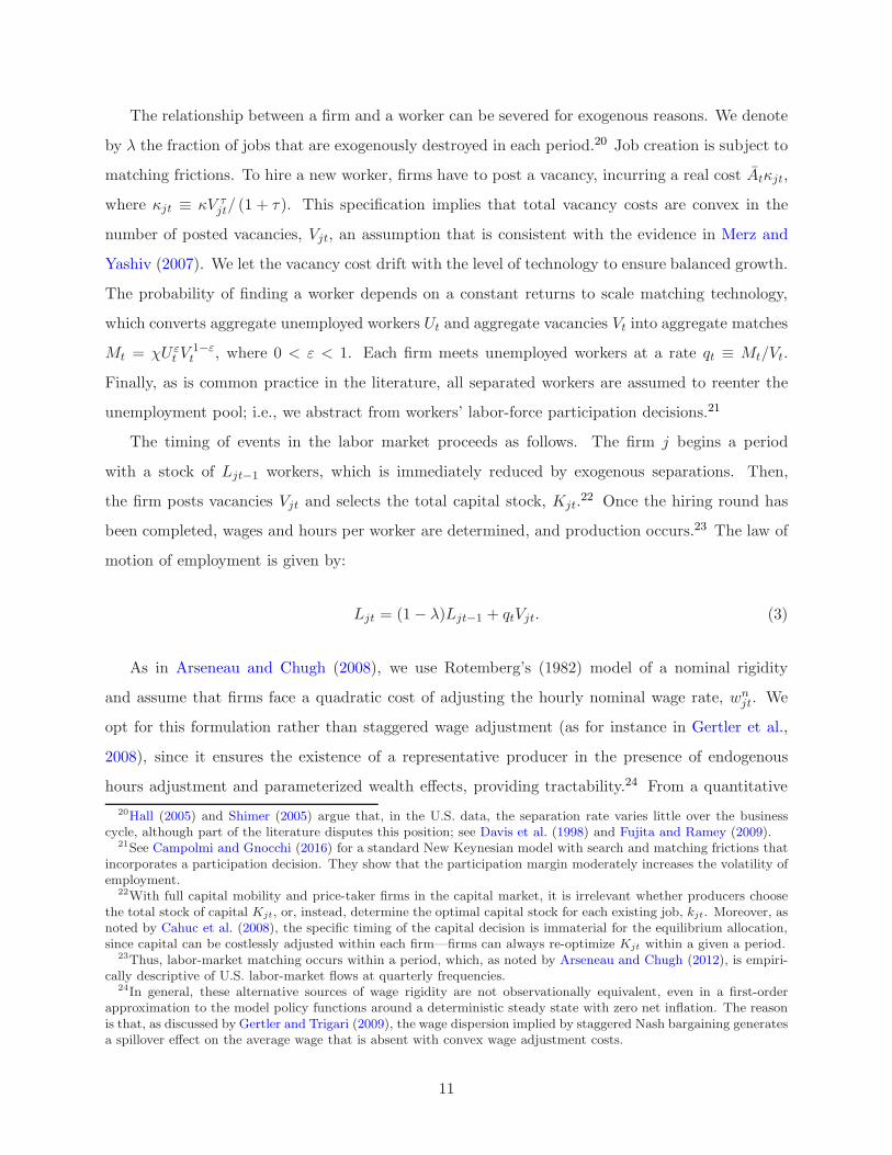
The relationship between a firm and a worker can be severed for exogenous reasons. We denote
by λ the fraction of jobs that are exogenously destroyed in each period.20 Job creation is subject to
matching frictions. To hire a new worker, firms have to post a vacancy, incurring a real cost Atκjt,
where κjt ≡ κV τjt/ (1 + τ). This specification implies that total vacancy costs are convex in the
number of posted vacancies, Vjt, an assumption that is consistent with the evidence in Merz and
Yashiv (2007). We let the vacancy cost drift with the level of technology to ensure balanced growth.
The probability of finding a worker depends on a constant returns to scale matching technology,
which converts aggregate unemployed workers Ut and aggregate vacancies Vt into aggregate matches
Mt = χU εt V
1−εt , where 0 < ε < 1. Each firm meets unemployed workers at a rate qt ≡ Mt/Vt.
Finally, as is common practice in the literature, all separated workers are assumed to reenter the
unemployment pool; i.e., we abstract from workers’ labor-force participation decisions.21
The timing of events in the labor market proceeds as follows. The firm j begins a period
with a stock of Ljt−1 workers, which is immediately reduced by exogenous separations. Then,
the firm posts vacancies Vjt and selects the total capital stock, Kjt.22 Once the hiring round has
been completed, wages and hours per worker are determined, and production occurs.23 The law of
motion of employment is given by:
Ljt = (1− λ)Ljt−1 + qtVjt. (3)
As in Arseneau and Chugh (2008), we use Rotemberg’s (1982) model of a nominal rigidity
and assume that firms face a quadratic cost of adjusting the hourly nominal wage rate, wnjt. We
opt for this formulation rather than staggered wage adjustment (as for instance in Gertler et al.,
2008), since it ensures the existence of a representative producer in the presence of endogenous
hours adjustment and parameterized wealth effects, providing tractability.24 From a quantitative
20Hall (2005) and Shimer (2005) argue that, in the U.S. data, the separation rate varies little over the businesscycle, although part of the literature disputes this position; see Davis et al. (1998) and Fujita and Ramey (2009).
21See Campolmi and Gnocchi (2016) for a standard New Keynesian model with search and matching frictions thatincorporates a participation decision. They show that the participation margin moderately increases the volatility ofemployment.
22With full capital mobility and price-taker firms in the capital market, it is irrelevant whether producers choosethe total stock of capital Kjt, or, instead, determine the optimal capital stock for each existing job, kjt. Moreover, asnoted by Cahuc et al. (2008), the specific timing of the capital decision is immaterial for the equilibrium allocation,since capital can be costlessly adjusted within each firm—firms can always re-optimize Kjt within a given a period.
23Thus, labor-market matching occurs within a period, which, as noted by Arseneau and Chugh (2012), is empiri-cally descriptive of U.S. labor-market flows at quarterly frequencies.
24In general, these alternative sources of wage rigidity are not observationally equivalent, even in a first-orderapproximation to the model policy functions around a deterministic steady state with zero net inflation. The reasonis that, as discussed by Gertler and Trigari (2009), the wage dispersion implied by staggered Nash bargaining generatesa spillover effect on the average wage that is absent with convex wage adjustment costs.
11
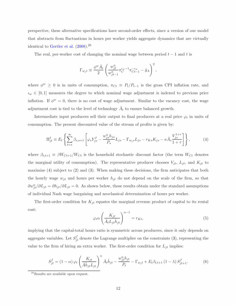
perspective, these alternative specifications have second-order effects, since a version of our model
that abstracts from fluctuations in hours per worker yields aggregate dynamics that are virtually
identical to Gertler et al. (2008).25
The real, per-worker cost of changing the nominal wage between period t− 1 and t is
Γwjt ≡φwAt
2
(wnjt
wnjt−1
πιw−1C π−ιw
Ct−1 − gA
)2
,
where φw ≥ 0 is in units of consumption, πCt ≡ Pt/Pt−1 is the gross CPI inflation rate, and
ιw ∈ [0, 1] measures the degree to which nominal wage adjustment is indexed to previous price
inflation. If φw = 0, there is no cost of wage adjustment. Similar to the vacancy cost, the wage
adjustment cost is tied to the level of technology At to ensure balanced growth.
Intermediate input producers sell their output to final producers at a real price ϕt in units of
consumption. The present discounted value of the stream of profits is given by:
ΠIjt ≡ Et
{∞∑
t=s
βs,s+1
[ϕsY
Ijs −
wnjshjs
PsLjs − ΓwjsLjs − rKsKjs − κAs
V 1+τjs
1 + τ
]}, (4)
where βt,t+1 ≡ βWCt+1/WCt is the household stochastic discount factor (the term WCt denotes
the marginal utility of consumption). The representative producer chooses Vjt, Ljt, and Kjt to
maximize (4) subject to (2) and (3). When making these decisions, the firm anticipates that both
the hourly wage wjt and hours per worker hjt do not depend on the scale of the firm, so that
∂wnjt/∂Ljt = ∂hjt/∂Ljt = 0. As shown below, these results obtain under the standard assumptions
of individual Nash wage bargaining and neoclassical determination of hours per worker.
The first-order condition for Kjt equates the marginal revenue product of capital to its rental
cost:
ϕtα
(Kjt
AtLjthjt
)α−1
= rKt, (5)
implying that the capital-total hours ratio is symmetric across producers, since it only depends on
aggregate variables. Let Sfjt denote the Lagrange multiplier on the constraints (3), representing the
value to the firm of hiring an extra worker. The first-order condition for Ljt implies:
Sfjt = (1− α)ϕt
(Kjt
AhjtLjt
)α
Athjt −wnjthjt
Pt− Γwjt + Etβt,t+1 (1− λ)Sf
jt+1. (6)
25Results are available upon request.
12

Intuitively, the value of a job to the firm corresponds to the expected, present discounted value of
the streams of profits from the match—the difference between the value of the marginal product
and the wage payment to the worker minus the cost of adjusting the nominal wage. Finally, the
first-order condition for vacancies equates the cost of filling a vacancy to the value of a filled position:
κAt
V τjt
qt= Sf
jt. (7)
Equations (6) and (7) imply a standard job creation condition:
κAtVτjt
qt= (1− α)ϕt
(Kjt
AhjtLjt
)α
Athjt −wnjthjt
Pt− Γwjt + κ (1− λ)Etβt,t+1
At+1Vτjt+1
qt+1.
Forward looking iteration of the job creation equation implies that, at the optimum, the expected
discounted value of the stream of profits generated by a match over its expected lifetime is equal
to the cost of filling a vacancy, κAtVτjt/qt.
Hours Determination
As is common practice in the literature, we assume that hours per worker maximize the joint
surplus of the firm and the worker.26 This implies that hjt adjusts to the point where the worker’s
marginal rate of substitution between consumption and leisure is equal to the value of the marginal
value product of an extra hour worked:
−Whjt
WCt= (1− α)ϕt
(kjt
ALjthjt
)α
At∆hjt,
where Whjtdenotes the worker’s marginal disutility from supplying an extra hour and
∆hjt≡
∂hjt∂hjt
=hjthjt
− φhhjt (hjt − hj) .
Using the first-order condition for capital, the optimal choice of hours per worker implies:
−Whjt
WCt= (1− α)ϕt
(rKt
ϕtα
) αα−1
At∆hjt. (8)
26Alternatively, we could assume that firms have the right to manage hours or consider Nash bargaining over hoursper worker. See footnote 36 in section 4 for a discussion of the performance of the model under these alternativeassumptions.
13

Notice that, while up to a first-order approximation hjt = hjt, the hours adjustment cost φh affects
aggregate dynamics through the term ∆hjt. Equation 8 shows that hjt only depends on aggregate
conditions, i.e., hjt = ht is invariant to the scale of the firm. Moreover, hjt does not directly depend
on the hourly wage wjt.
Wage Bargaining
The nominal wage is the solution to an individual Nash bargaining problem, and the wage payment
divides the match surplus between workers and firms. Due to the presence of nominal rigidities,
we assume that bargaining occurs over the nominal wage rather than the real wage, as in Arseneau
and Chugh (2008), Gertler et al. (2008), and Thomas (2008). With zero costs of nominal wage
adjustment (φw = 0), the real wage is identical to the one obtained from bargaining directly over
the real wage. This is no longer the case in the presence of wage adjustment costs. As is standard
practice in the literature, the wage bargaining is atomistic, implying that the firm and the worker
take Kjt and Ljt as given at the bargaining stage. Moreover, both parties account for the fact that
∂ht/∂wjt = 0, as shown above.
Let ηt ∈ (0, 1) be the weight given to the worker’s individual surplus in Nash bargaining. We
assume that ηt follows the process: log ηt = ρη log ηt−1+(1− ρη) log η+ εηt, where εηtiid∼ N
(0, σ2
η
).
Exogenous fluctuations in the worker’s bargaining power are the counterpart of wage-markup shocks
typically assumed in the estimation of New Keynesian models that abstract from search and match-
ing frictions.27 The firm and the worker maximize the Nash product(Sfjt
)1−ηt (Swjt
)ηt
, where Sfjt
is defined as in (6) and Swjt denotes the worker surplus:
Swjt =
wnjt
Ptht − bAt +
WLt
WCt+ Et
[βt,t+1 (1− λ)Sw
jt+1
(1−
Mt+1
Ut+1
)]. (9)
where WLt is the disutility from working. The worker’s surplus corresponds to the expected present
discounted value of wage payments over the lifetime of the match minus the expected present
discounted value of the flow value of unemployment, including unemployment benefits from the
government bAt (financed with lump sum taxes), and the utility gain from leisure in terms of
consumption, WLt/WCt.
The first-order condition with respect to wnjt implies the following sharing rule: ηwjtS
fjt =
27Up to a first-order approximation, wage markup shocks are isomorphic to hours supply shocks in the conventionalNew Keynesian model. Such equivalence breaks down in the presence of labor-market search and matching frictions.
14

(1− ηwjt)Swjt, where ηwjt is the effective bargaining share of workers:
ηwjt ≡ηtht
ηtht − (1− ηt)(∂Sf
jt/∂wnjt
) .
(See Appendix B for the expression of ∂Sfjt/∂w
njt.) As in Gertler and Trigari (2009), the effective
bargaining share is time-varying due to the presence of wage adjustment costs. Absent these
costs, the bargaining share is exogenous, ηwjt = ηt. Importantly, wage rigidity implies that ηwjt is
countercyclical, amplifying employment fluctuations in response to aggregate shocks as first noted
by Gertler and Trigari (2009).
It is straightforward to verify that wnjt does not depend on the scale of the firm. To see this,
substitute equation (8) into the definition of the worker’s and firm’s surplus, Swjt and Sf
jt, and use
the first-order condition for capital to eliminate the capital-labor ratio in Sft . Then, since all the
intermediate firms produce with identical technology At, there is a symmetric equilibrium in which
Kjt = Kt, Ljt = Lt, hjt = ht, Vjt = Vt, and wnjt = wn
t . In turn, nominal hourly wage inflation,
defined by πwt ≡ wnt /w
nt−1 is linked to CPI inflation by πwt = (wt/wt−1) πCt, where wt ≡ wn
t /Pt
denotes the real hourly wage. Finally, searching workers in period t are equal to the mass of
unemployed workers: Ut = 1− (1− λ)Lt−1.
Final Goods Production
A continuum of monopolistically competitive final-sector firms produce differentiated varieties us-
ing the intermediate input. The producer ω faces the following demand: Y Cωt = (Pωt/Pt)
−θt Y Ct ,
where Y Ct denotes aggregate demand of the final consumption basket, inclusive of sources besides
household consumption.
We introduce price-setting frictions by following Rotemberg (1982) and assume that final pro-
ducers must pay a quadratic price adjustment cost. We also allow for price indexation by assuming
that final producers index price changes to past CPI inflation, so that price adjustment costs take
the form:φp
2
(Pωt
Pωt−1πιp−1C π
−ιpCt−1 − 1
)2
PωtYCωt ,
where φp ≥ 0 determines the size of the adjustment cost (prices are flexible if φp = 0) and ιp ∈ [0, 1]
is the indexation parameter.
Optimal price setting implies that the (real) output price Pωt/Pt is equal to a markup over the
15

real marginal cost ϕt:Pωt
Pt=
θt(θt − 1
)Ξωt
ϕt,
where
Ξωt ≡ 1−φp
2
(πωtπ
−ιpCt−1π
ιp−1C − 1
)2+
φp
θt − 1
πιp−1C
(πωtπ
−ιpCt−1π
ιp−1C − 1
)πωtπ
−ιpCt−1
−Et
[βt,t+1
(πωt+1π
−ιpCt π
ιp−1C − 1
)π−1Ct+1π
2ωt+1π
−ιpCt
Y Cωt+1
Y Cωt
]
,
where πωt ≡ Pωt/Pωt−1. There are two sources of endogenous markup variation in the model. First,
the cost of adjusting prices gives firms an incentive to change their markups over time in order to
smooth price changes across periods. Second, exogenous shocks to the firms’ market power result
in time-varying markups even in the absence of price stickiness. In the symmetric equilibrium,
Pωt = Pt and Ξωt = Ξ. As a consequence, πωt = πt = πCt.
Household Budget Constraint and Optimal Intertemporal Decisions
The household enters period t with nominal private bond holdings Bt, earning a gross interest rate
it. The household also accumulates physical capital and rents it to intermediate input producers
in a competitive capital market. Investment in the physical capital stock, IKt, requires the use of
the same composite of all available varieties as the basket Ct. We introduce convex adjustment
costs in physical investment and variable capital utilization. The utilization rate of capital is set
by the household. Thus, effective capital rented to firms, Kt, is the product of physical capital,
Kt, and the utilization rate, uKt: Kt = uKtKt. Increases in the utilization rate are costly because
higher utilization rates imply faster capital depreciation. We assume a standard convex depreciation
function: δKt = δ0 + δ1 (uKt − 1) + δ2 (uKt − 1)2. Physical capital, Kt, obeys a standard law of
motion:
Kt+1 = (1− δKt) Kt + PKt
[1−
νK2
(IKt
IKt−1− gA
)2]IKt, (10)
where νK > 0 is a scale parameter, and PKt is an investment specific shock. The latter is a source
of exogenous variation in the efficiency with which the final good can be transformed into physical
capital, and thus into tomorrow’s capital input.28 The investment shock evolves via the process
log PKt = ρPKlog PKt−1 + εPK t, where εPK t
iid∼ N
(0, σ2
PK
).
28Justiniano et al. (2010) suggests that this variation might stem from technological factors specific to the produc-tion of investment goods, but also from disturbances to the process by which these investment goods are turned intoproductive capital.
16

The per-period household’s budget constraint is:
PtCt+PtIKt+Bt+1 = itBt+wnt htLt+rKtPtKt+bAt (1− Lt)Pt+PtΠ
It +Pt
∫ 1
0ΠF
t (i) di+T gt , (11)
where T gt is a nominal lump-sum tax from the government.
The household maximizes its expected intertemporal utility subject to (10) and (11). The
Euler equation for capital accumulation requires: ζKt = Et {βt,t+1 [rt+1uKt+1 + (1− δKt+1) ζKt+1]},
where ζKt denotes the shadow value of capital (in units of consumption), defined by the first-order
condition for investment IKt:
ζ−1Kt =
[1−
νK2Γ2IKt − νKΓIKt (ΓIKt + 1)
]+ νKβt,t+1Et
[ζKt+1
ζKt(ΓIKt+1) (ΓIKt+1 + 1)2
],
where ΓIKt ≡ (IKt/IKt−1) − 1. The optimal condition for capital utilization implies: rKt =
ζKt[δK1+δK2(uKt−1)]. Finally, the Euler equation for bond holdings implies: 1 = itEt [βt,t+1/ (1 + πCt+1)].
The Government and Market Clearing
Fiscal policy is fully Ricardian. The government finances its budget deficit with lump-sum taxes
each period. Public spending is determined exogenously, Gt = gt, where the exogenous government
spending shock gt follows the process log gt = ρg log gt + (1− ρg) log g + εgt, with εgtiid∼ N
(0, σ2
g
).
The monetary authority sets the nominal interest rate following a feedback rule of the form
iti=
(it−1
i
)i [(πCt
πC
)π (Ygt
Yg
)Y]1−i ( Ygt
Ygt−1
)dY
ıit, (12)
where i is the steady state of the gross nominal interest rate. The interest rate responds to deviations
of inflation and the GDP gap, Ygt, from their long-run targets, as well as to deviations of the
growth rate of the GDP gap, Ygt/Ygt−1. GDP is defined as Yt ≡ Ct + IKt + Gt. Consistent with
Woodford (2003), we define the GDP gap as the deviation of model GDP from its level prevailing
under flexible prices and wages and absent inefficient shocks (i.e., absent markup and bargaining
power shocks). The monetary policy rule is subject to a shock, ıit, which evolves according to
log ıit = ρı log ıit−1 + εıt, with εitiid∼ N
(0, σ2
ı
).
In the symmetric equilibrium, bonds are zero in net supply: Bt = Bt+1 = 0. Thus, combin-
ing the household’s and government’s budget constraints yields the following aggregate resource
constraint:
Y Ct
[1−
ν
2
(πCtπ
ιp−1C π
−ιpCt−1 − 1
)2]= Ct + IKt + κtAtVt +Gt. (13)
17

Intuitively, total output produced by firms must be equal to the sum of market consumption,
investment in physical capital, the costs associated to job creation, the purchase of goods from the
government, and the real cost of changing prices. Finally, labor market clearing implies Y Ct = Y I
t .
The model contains 15 equations that determine 15 endogenous variables: it, πCt, πwt, Ct, Lt,
Vt, Mt, ht, wt, ϕt, Kt+1, IKt, ζKt, uKt, rKt, and 15 definitions (Ut, Sft , S
wt , ht, qt, WCt, Wht,
WLt, hjt, ∆ht, δKt, κt, ηwt, Ξt, and Ygt). As detailed below, the terms WCt, Wht, and WLt depend
on the specification of the household’s utility, u (·). Additionally, the model features 8 exogenous
disturbances: gAt, βt, ht, θt, ηt, PKt, ıt, and gt. Consumption, investment, capital, the real wage,
and GDP, (together with Y Ct , Sf
t , Swt , andWCt) fluctuate around a stochastic balanced growth path,
since the level of technology has a unit root. We rewrite the model in terms of detrended variables
and compute the log-linear approximation around the non-stochastic steady state. The details
of these steps can be found in Appendix C, along with the full set of stationarized equilibrium
conditions (and their log-linear approximations). We then solve the resulting linear system of
rational expectation equations to obtain the transition equations, which are linked to data with an
observation equation to form the state-space model used for estimation.
4 Baseline Model: Separable Preferences and Frictionless Hours Adjustment
We first estimate a model that corresponds to the baseline version considered in the literature:
separable preferences and frictionless hours-per-worker adjustment—see for instance, Andolfatto
(1996), Arseneau and Chugh (2008), Christiano et al. (2011), Merz (1995), Ravenna and Walsh
(2012), and Trigari (2009). We set φh = 0 and assume that
Wt ≡ Et
∞∑
s=t
βs−tβs
[log(Ct − hCCt−1)− ht
∫ Lt
0
h1+ωjs
1 + ωdj
],
where hC is the degree of habit formation. Consumption utility is logarithmic to ensure the existence
of a balanced growth path in the presence of non-stationary technological progress. This preference
specification implies that disutility of labor supply isWLt = −βthth1+ωjt / (1 + ω), while the marginal
disutility of working an extra hour is Whjt= −βthth
ωjt. Table A.3 summarizes the equilibrium
conditions of the baseline model.
We estimate the model with U.S. quarterly data from 1965:1 to 2007:4. Details of the data
construction and linkages to observables are presented in Appendix A. For the baseline estimation,
18

we end the estimation prior to the recent zero lower bound episode.29 Our initial estimation
includes seven observables commonly employed in the literature: the log difference of aggregate
consumption, investment, GDP, and real wages, the log difference of the GDP deflator, the Federal
Funds rate, and the log of economy-wide total hours worked. 30 To avoid stochastic singularity, we
include seven structural shocks. To facilitate comparison with the literature (i.e., Christiano et al.,
2011, and Gertler et al., 2008), our baseline specification assumes that shocks to the exogenous
component of the worker’s bargaining power, ηt, are the only disturbance directly affecting the
labor market, i.e., ht = 1 for any t.31
In addition, we estimate the model including the hours supply shock, ht, and one ancillary
observable, the log of economy-wide employment.32 Using information on both margins of labor
adjustment helps identify key labor parameters such as the Frisch elasticity. Moreover, the inclusion
of the hours supply shock gives the model a better chance to match the dynamics of the labor
margins.
We use Bayesian inference methods to construct the parameters’ posterior distribution, which
is a combination of a prior density for the parameters and the likelihood function, evaluated using
the Kalman filter. We take 1.5 million draws from the posterior distribution using the random
walk Metropolis-Hastings algorithm. For inference, we discard the first 500, 000 draws and keep
one every 50 draws to remove some correlation of the draws.33
Prior Distributions
We impose dogmatic priors for some parameters. The household discount factor β is set to 0.99,
α is 0.3, and depreciation δ is 0.025. The steady-state price markup is set at 1.1. Steady-state
government spending is fixed at 20 percent of GDP, which equals the post-war average for all levels
of government spending. Following standard practice in the literature, we use independent evidence
for the average quarterly separation rate λ and the elasticity of matches to unemployment, ε. In
particular, we choose λ = 0.105 based on the observation that jobs last on average about two
29See Hirose and Inoue (2015) for a discussion of how the ZLB can bias estimates of log-linearized model parameters.30Examples include Christiano et al. (2005), Smets and Wouters (2007), Del Negro et al. (2007), Gertler et al.
(2008), and Justiniano et al. (2010).31In section 7, we discuss the alternative possibility of focusing on stochastic fluctuations in the disutility of hours
worked, ht, while keeping constant the worker’s bargaining power, i.e., ηt = 1.32This is observationally equivalent to estimating the model using hours per worker and employment as observables,
since we abstract from measurement error.33We set the step size to ensure the acceptance rate is in the range of 20 to 40 percent for all variations of
the estimated model. Convergence diagnostics include cumulative sum of draws (cumsum) statistics and Geweke’sSeparated Partial Means (GSPM) test. Results are available from the authors.
19

and half years in the U.S. economy (Shimer, 2005). We set ε to be equal to 0.5, the midpoint of
the evidence typically cited in the literature and within the range of plausible values (0.5 to 0.7)
reported by Petrongolo and Pissarides (2006). Finally, we set the cost of posting a vacancy, κ, and
the matching efficiency parameter, χ, to match the quarterly average job finding probability, M/U ,
and the average probability of filling a vacancy, q. For the U.S., the former is equal to 0.95, while
the latter is 0.9 (Shimer, 2005).
Table 2 lists the prior distributions for the remaining parameters in the columns labeled “Priors.”
Our priors for common parameters are similar to those in Smets and Wouters (2007). We set the
price stickiness parameter, φp, to a value that would replicate the frequency of price adjustment in
a Calvo-type Phillips curve in the absence of strategic price complementarities. For comparability
with the literature, we directly estimate the related Calvo parameter ξp.34 In contrast, no direct
mapping to a Calvo-type wage Phillips curve exists, even in a linearized setup. Thus, we employ
a prior for φw that permits a broad degree of stickiness. The estimated labor market parameters
include the steady-state value of the workers’ bargaining power η, the replacement rate b/wh, and
the degree of convexity in the cost of posting vacancies τ . The first two have priors similar to
those in Gertler et al. (2008). Finally, the bargaining power, price markup, and investment shocks
are normalized to enter with a unitary coefficient in the log-linearized equations that determine
wages, inflation, and investment, respectively. The priors for the standard deviations of shocks are
chosen to generate similar volatilities between the variables they directly impact and their data
counterparts, as is common practice in the literature.
Posterior Estimates
Table 2 reports the posterior estimates of the baseline model presented in section 3. As previ-
ously discussed, we estimate two versions of this model. The first includes seven observables and
seven shocks: TFP, investment, preference, government spending, interest rate, price markup, and
bargaining shocks. Parameter estimates from this version are listed under the column “7 obs.”
The second version includes an additional observable, employment, and an additional labor market
shock, the hours-supply shock ht. Parameter estimates from this version are listed in the column
“Baseline” under the headings “8 obs” in Table 2. For a discussion of the posterior estimates
relative to the literature, see Appendix D.
34ξp is related to φp via the mapping φp =[(
θ − 1)
/θ]
ξp/(1− ξp)(1− ξpβ).
20

Table 2: Posterior Distributions for Estimated Parameters.Parameter Prior Posterior
7 obs 8 obs
Baseline Baseline Preferred
Model Model Model
Dist.* Mean Std. Mean 90% Int Mean 90% Int Mean 90% Int
Preferences
hC , habit formation B 0.5 0.1 0.79 [0.73, 0.83] 0.68 [0.63, 0.72] 0.79 [0.73, 0.84]ω, inverse Frisch G 2 0.5 3.34 [2.49, 4.33] 6.98 [5.83, 8.24] 2.74 [1.94, 3.68]
Frictions and Production
100 log gA, growth rate N 0.4 0.03 0.41 [0.37, 0.45] 0.40 [0.36, 0.44] 0.41 [0.36, 0.45]νK , investment adj. cost N 4 1.5 4.89 [3.15, 6.93] 6.97 [5.48, 8.54] 7.76 [6.10, 9.50]φh, hours adj. cost N 4 1.5 n.e. n.e. 6.17 [4.53, 7.91]ς, capital utilization B 0.5 0.1 0.54 [0.45, 0.62] 0.51 [0.43, 0.58] 0.44 [0.36, 0.52]η, workers bargaining power B 0.5 0.1 0.76 [0.63, 0.86] 0.56 [0.44, 0.68] 0.50 [0.38, 0.62]b/(w ∗ h), replacement rate B 0.5 0.1 0.59 [0.48, 0.69] 0.56 [0.41, 0.69] 0.47 [0.34, 0.58]τ , convexity vacancy cost G 2 0.5 1.27 [0.80, 1.83] 2.67 [2.05, 3.38] 2.74 [2.10, 3.48]φw/1000, wage stickiness N 2 0.4 2.86 [2.31, 3.42] 2.53 [2.00, 3.07] 2.59 [2.07, 3.13]ιw, wage partial indexation B 0.5 0.15 0.77 [0.61, 0.90] 0.69 [0.54, 0.84] 0.71 [0.56, 0.85]ξp, price stickiness B 0.66 0.1 0.86 [0.83, 0.89] 0.90 [0.87, 0.93] 0.90 [0.87, 0.93]ιp, price partial indexation B 0.5 0.15 0.13 [0.06, 0.21] 0.12 [0.05, 0.21] 0.12 [0.05, 0.21]
Monetary policy
π , interest resp. to inflation N 1.7 0.3 1.78 [1.55, 2.05] 1.21 [1.01, 1.43] 1.32 [1.12, 1.53]Y , interest resp. to Y gap G 0.125 0.1 0.05 [0.02, 0.09] 0.10 [0.06, 0.14] 0.07 [0.03, 0.12]dY , interest to Y gap growth N 0.13 0.05 0.34 [0.28, 0.40] 0.31 [0.25, 0.36] 0.28 [0.23, 0.34]i, resp. to lagged interest rate B 0.75 0.1 0.76 [0.72, 0.80] 0.73 [0.68, 0.77] 0.75 [0.70, 0.79]
Shocks
ρgA , technology B 0.5 0.2 0.14 [0.05, 0.24] 0.07 [0.02, 0.13] 0.10 [0.03, 0.19]
ρβ , preference B 0.5 0.2 0.70 [0.59, 0.79] 0.84 [0.78, 0.89] 0.67 [0.52, 0.79]ρPK
, investment B 0.5 0.2 0.84 [0.78, 0.90] 0.20 [0.10, 0.30] 0.20 [0.11, 0.30]
ρθ, price markup B 0.5 0.2 0.88 [0.81, 0.93] 0.82 [0.74, 0.88] 0.85 [0.77, 0.91]ρη, bargaining B 0.5 0.2 0.37 [0.24, 0.51] 0.16 [0.06, 0.26] 0.16 [0.07, 0.27]ρg, govt cons B 0.5 0.2 0.99 [0.98, 0.99] 0.99 [0.98, 0.99] 0.98 [0.98, 0.99]ρı, monetary shock B 0.5 0.2 0.13 [0.05, 0.22] 0.15 [0.06, 0.25] 0.16 [0.07, 0.26]ρh, hours shock B 0.5 0.2 n.e. 0.97 [0.94, 0.98] 0.97 [0.96, 0.99]100σgA
, technology IG 0.5 1 0.83 [0.75, 0.92] 1.01 [0.92, 1.11] 1.07 [0.97, 1.19]
100σβ , preference IG 1 1 2.43 [2.00, 2.95] 2.06 [1.78, 2.39] 2.87 [2.30, 3.63]100σPK
, investment IG 0.1 1 0.71 [0.60, 0.83] 1.36 [1.18, 1.56] 1.37 [1.19, 1.57]
100σθ , price markup IG 0.1 1 0.06 [0.05, 0.07] 0.06 [0.05, 0.08] 0.06 [0.05, 0.07]100ση , bargaining IG 1 1 4.11 [3.36, 4.88] 4.90 [4.28, 5.56] 4.88 [4.27, 5.52]100σg , govt cons IG 0.5 1 1.47 [1.34, 1.61] 1.53 [1.39, 1.67] 1.57 [1.43, 1.72]100σı, monetary shock IG 0.1 1 0.24 [0.21, 0.26] 0.24 [0.22, 0.27] 0.24 [0.21, 0.26]100σh, hours supply shock IG 0.5 1 n.e. 3.49 [2.97, 4.05] 3.51 [2.93, 4.17]
Implied from Estimated Model
βh [0.03, 0.22] [0.16, 0.76] [0.13, 0.56]βL [0.64, 1.21] [0.22, 0.89] [0.20, 0.71]βcov [-0.35, 0.25] [-0.43. 0.37] [-0.05, 0.44]Log marginal data density -1073 -10242 ln(Bayes Factor) 98 0vs. Preferred
*Distributions: N: Normal; G: Gamma; B: Beta; IG: Inverse Gamma.
21

0 1 2 3 4 5
0
0.5
1
corr(Yt,Y
t−k)
0 1 2 3 4 5
−0.2
0
0.2
0.4
0.6
corr(Yt,C
t−k)
0 1 2 3 4 5−0.4
−0.2
0
0.2
corr(Yt,TH
t−k)
0 1 2 3 4 5−0.4
−0.2
0
0.2
corr(Yt,L
t−k)
0 1 2 3 4 5
−0.2
0
0.2
corr(Yt,h
t−k)
0 1 2 3 4 5
0
0.2
0.4
0.6
corr(Ct,Y
t−k)
0 1 2 3 4 5
0
0.5
1
corr(Ct,C
t−k)
0 1 2 3 4 5
−0.2
0
0.2
0.4
corr(Ct,TH
t−k)
0 1 2 3 4 5
−0.2
0
0.2
0.4
0.6
corr(Ct,L
t−k)
0 1 2 3 4 5−0.6−0.4−0.2
00.20.4
corr(Ct,h
t−k)
0 1 2 3 4 5
0.2
0.4
0.6
corr(THt,Y
t−k)
0 1 2 3 4 5
0
0.2
0.4
corr(THt,C
t−k)
0 1 2 3 4 5
0.6
0.8
1
corr(THt,TH
t−k)
0 1 2 3 4 5
0.2
0.4
0.6
0.8
corr(THt,L
t−k)
0 1 2 3 4 5−0.2
00.20.40.60.8
corr(THt,h
t−k)
0 1 2 3 4 50
0.2
0.4
corr(Lt,Y
t−k)
0 1 2 3 4 5
0.2
0.4
0.6
corr(Lt,C
t−k)
0 1 2 3 4 5
0.2
0.4
0.6
0.8
corr(Lt,TH
t−k)
0 1 2 3 4 5
0.4
0.6
0.8
1
corr(Lt,L
t−k)
0 1 2 3 4 5−0.4−0.2
00.20.40.6
corr(Lt,h
t−k)
0 1 2 3 4 5
−0.2
0
0.2
0.4
corr(ht,Y
t−k)
0 1 2 3 4 5−0.6
−0.4
−0.2
0
0.2
corr(ht,C
t−k)
0 1 2 3 4 5
00.20.40.60.8
corr(ht,TH
t−k)
0 1 2 3 4 5
−0.4
−0.2
0
0.2
0.4
corr(ht,L
t−k)
0 1 2 3 4 5
0.4
0.6
0.8
1
corr(ht,h
t−k)
Figure 2. Correlograms from the data (solid lines) and 90 percent posterior intervals from 1) the baselinemodel with seven observables (dotted dashed lines) and 2) the baseline model with eight observables (dashedlines).
Model Fit
To understand how well the baseline model fits the data, we compare a set of statistics implied by
the model to their data counterparts. Figure 2 plots the correlogram for several aggregate macroe-
conomic and labor market variables in the data (solid lines), as well as the 90-percent posterior
intervals implied by both parameter and small sample uncertainty from the seven observable case
(dotted lines) and the eight observable case (dashed lines).35 We discuss the results of each case in
turn.
The literature shows that the baseline model with only the extensive margin and seven observables—
35We sample 10,000 draws from the posterior. For each parameter draw, we generate 100 samples of the observablevariables from the model with the same length as our dataset, after first discarding 100 initial observations. Wecompute statistics for each of these samples.
22
including either total hours or employment—is able to reproduce the joint dynamics of employment
and macroeconomic variables (see, for instance, Gertler et al., 2008). Estimates of a version of our
baseline model with only the extensive margin are in line with these results (results available upon
request). However, when the intensive margin is introduced in the model, its ability to account for
the correlations between labor market variables and aggregate macroeconomic series is significantly
impaired, as evidenced by comparing the data (solid lines) and model (dotted lines) statistics in
figure 2. First, the baseline model estimated with seven observables does not capture the positive
correlation between hours and employment nor the relative contributions of the labor margins to
the variance of total hours. In particular, the model assigns an almost exclusive role to employ-
ment, as the 90 percent posterior bands for the share of the labor margin to the variance of total
hours (βL) are between 0.64 and 1.21 (see Table 2), while the data counterpart is only 0.51. The
βcov ranges from −0.35 to 0.25, well short of the positive comovement (0.31) between hours and
employment observed in the data. Moreover, the model overstates the correlation between the
growth rate of output with total hours or employment at various leads and lags. Even though it
correctly reproduces the correlogram between total hours and consumption growth, it does so with
a counterfactual comovement of the individual margins with respect to consumption.
Prima facie, the poor performance of the model with seven observables could reflect that the
model is estimated with only one labor market observable. However, simply adding information
about the labor market by increasing the set of observables to include simultaneously employment
(or hours per worker) and total hours does not improve the performance of the model. The dashed
lines of figure 2 report the 90 percent posterior correlogram bands for the baseline model when
employment data and an hours supply shock are incorporated in the estimation. The correlation of
hours per worker and consumption growth is still too low relative to the data, while the correlation
between employment and output growth is instead too high. Despite providing more information
about labor market dynamics, the model still fails to ensure the positive correlation between hours
and employment, and the βcov ranges from −0.43 to 0.37 (see Table 2). In addition, this version
of the model tends to overstate the importance of hours per worker relative to the data, as the
posterior for βh ranges from 0.16 to 0.76, whereas its value is 0.18 in the data. All in all, the baseline
model—independently of the shocks considered or the observables included in the estimation—is
unable to replicate satisfactorily the correlation structure between the aggregate macroeconomic
series and the labor market variables.
23

The main issue is that hours per worker tends to be too countercyclical in the model.36 As
detailed in Appendix E, such counterfactual correlations reflect the negative comovement between
the labor margins following standard supply and demand shocks, as well as in response to labor
market shocks (either wage-bargaining shocks or hours-supply shocks). In particular, hours per
worker fall in response to both positive technology and demand shocks, since wealth effects reduce
labor supply. By contrast, employment rises, since the surplus of hiring a worker increases in the
presence of nominal and real wage rigidities. Moreover, the response of hours per worker is as large
as employment for several of the shocks we consider.
As a final check on the performance of the baseline model, we perform the following counter-
factual. We use the posterior mean estimates from the baseline model with seven observables to
obtain model time-series using the two-sided Kalman filter. Figure 3 displays the model-implied la-
bor market variables (dashed lines), as well as the data (dotted-dashed lines). Since total hours are
included as an observable, by construction the two-sided Kalman filter ensures the baseline model
perfectly matches this series. However, the model matches total hours only with counterfactual
employment and hours per worker series, suggesting short-comings in the internal propagation of
the model.
To address the shortcomings of the baseline model, in the next section we propose two mod-
ifications that reconcile the model with the data. First, we introduce preferences with a flexible
parametrization of the strength of the short-run wealth effect on hours supply. In addition, to
discipline the movement in hours worked, we allow for non-zero adjustment costs to the intensive
margin, φh. These two ingredients provide a parsimonious strategy to reproduce the correlation of
the labor market variables and the macroeconomic series.
5 Alternative Model: Parametrized Wealth Effects and Costly Hours
Adjustment
This section contains the econometric analysis of the model with alternative preferences and hours
adjustment costs, which we reference as our preferred model. We first introduce the alternative
36Notice that under the alternative assumption that firms have the right to manage (RTM) hours, hours supplyconsiderations (and thus wealth effects) do not affect ht. Nevertheless, an estimated version with RTM verifies thatthe lack of positive comovement between Lt and ht persists—under RTM, ht equates the marginal product of anhour worked to wt, implying that, with wage rigidities and pre-determined capital, ht falls when Lt increases, otherthings equal. In contrast, the comovement between ht and Lt improves with Nash bargaining over hours per worker,as long as the worker’s bargaining share is not constrained to be symmetric to the corresponding share in wage Nashbargaining. This result reflects the additional degree of freedom stemming from the extra bargaining parameter.Results are available upon request.
24

1965 1975 1985 1995 2005-10
-8
-6
-4
-2
0
2
4
6
8
10Employment
1965 1975 1985 1995 2005
-8
-6
-4
-2
0
2
4
6
Total Hours
1965 1975 1985 1995 2005-4
-3
-2
-1
0
1
2
3
4Hours per Worker
Figure 3. Fitted and counterfactual variables. Blue dashed lines are simulated from the posterior meanestimates of the baseline model with seven structural shocks. Red dotted-dashed lines denote the data.
functional form for the household’s utility. Next, we discuss priors on new parameters and assess
the fit of the model relative to the data.
Parametrized Wealth Effects in Labor Supply
We modify the period utility function to encompass an alternative preference specification that
features a flexible parameterization of the strength of the short-run wealth effect on the labor
supply. We consider the class of preferences first introduced by Jaimovich and Rebelo (2009) (JR
henceforth). Following Schmitt-Grohe and Uribe (2007), we modify the original JR specification to
allow for internal consumption habit formation. The period utility function of the representative
household now is given by:
Wt ≡ Et
∞∑
s=t
βs−tβs
[log
(Ct − hCCt−1 − htXt
∫ Lt
0
h1+ωjt
1 + ωdj
)], (14)
where γ ∈ (0, 1] and Xt = (Ct − hCCt−1)γ X1−γ
t−1 . The parameter γ governs the magnitude of the
wealth elasticity of labor supply. As γ → 0, in the absence of habit formation, and abstracting
from time variation in the number of employed family members, this is the preference specification
considered by Greenwood et al. (1988). This special case induces a supply of labor that is indepen-
dent of the marginal utility of consumption. As a result, when γ is small, anticipated changes in
25

income will not affect the current labor supply. As γ increases, the wealth elasticity of labor supply
rises. In the polar case in which γ is unity, per-period utility becomes a product of habit-adjusted
consumption and a function of hours worked.37
Notice that the marginal disutility from labor supply, Whjt, now is defined as:
Whjt≡ −Ψ−1
t βththωjtXt,
where Ψt ≡ Ct − hCCt−1 − htXt
∫ Lt
0
[h1+ωjt / (1 + ω)
]dj. Thus, the marginal rate of substitu-
tion between hours and consumption for worker j, −Whjt/WCt, continues to depend on aggregate
variables, with the exception of hours worked, hjt. As a result, equation (8) implies that hours
per worker, hjt, continue to depend only on aggregate conditions, so that hjt = ht (and thus
hjt = ht). Moreover, relative to the baseline model, the equilibrium wage differs only because of
the different definitions of the value of the marginal product of labor and the flow value of unem-
ployment implied by the parametrized wealth effect on the labor supply. In particular, we now
have WLt = −Ψ−1t βthth
1+ωt Xt.
Overall, our modifications affect three equilibrium conditions—equations (4), (14), and (15) in
Table A.3—and three definitions—equations D.4-D.6 in Table A.3 in Appendix C.
Estimation and Model Performance
We estimate the model with the same eight observables discussed above. For symmetry, we employ
the same prior for hours adjustment costs as for investment adjustment costs, a normal distribution
centered at 4 with a standard deviation of 1.5. This prior is diffuse enough to allow positive mass
over a wide range of low and high adjustment cost values. We use a dogmatic prior for the parameter
governing the strength of the wealth effect in labor supply, setting γ = 0.01. This value is sufficiently
small to approach the limiting case of no wealth effects. In addition, we also estimate a version of
the model with a Beta prior for γ centered at 0.5 with a standard deviation of 0.1. The posterior
mean for γ in this case is 0.16, outside the 90 percent prior bands. Lowering the prior mean of γ
results in lower posterior estimates and similar transmission mechanisms as our calibrated version.
The priors for the remaining parameters are the same as those discussed in Section 4.
37The presence of employed and unemployed workers implies that even with full risk-sharing within the household,the specification in equation (14) cannot be obtained by aggregating primitive utility functions for employed andunemployed workers. We have considered an alternative version of the model that features JR preferences foremployed workers and a distinct utility function for unemployed family members. We then aggregate across agents,maintaining the assumption of full risk sharing within the household. Details are available upon request.
26

Table 2 reports the log marginal data densities and Bayes factors for the baseline and preferred
models. Bayes factors quantify the relative support of two competing specifications given the
observed data and are calculated from marginal data densities. Log marginal data densities are
computed using Geweke’s (1999) modified harmonic mean estimator with a truncation parameter
of 0.5.38 Kass and Raftery (1995) suggest that if twice the natural logarithm of the Bayes factor
is greater than 2, then there is positive evidence in favor of the first model. Values greater than
10 suggest very strong evidence. The baseline model has a value substantially larger than 10,
suggesting the data have strong preference for the model with JR preferences and hours adjustment
costs. Furthermore, as shown in section 7, including only JR preferences or hours adjustment costs
improves the model fit relative to the baseline model, while the inclusion of both is strongly preferred
by the data.
Figure 4 plots the correlogram for several aggregate macroeconomic and labor market variables
in the data (solid lines), as well as the 90 percent posterior intervals implied by both parameter
and small sample uncertainty from this preferred model (dotted lines) and the baseline model
with eight observables (dashed lines). In almost all cases, the correlogram bands for the preferred
model encapsulate the data counterparts, whereas the baseline model often fails to account for the
cross-correlation structure of labor variables and macroaggregates. The preferred specification also
implies variance decompositions of total hours more united with the data counterparts (see Table
2): βh ranges from 0.12 to 0.54, βL from 0.20 to 0.72, and βcov from −0.05 to 0.44.
The inclusion of JR preferences significantly improves the performance of the model. As de-
scribed in the previous section, JR preferences reduce the strength of the short-run wealth effect
on the labor supply. This mitigates the effect of variations in consumption on the marginal rate of
substitution and makes hours per worker more responsive to changes in the value of the marginal
product of hours. In turn, the increased comovement between hours per worker and employment
strengthens the comovement of hours per worker with both output and investment. This also ex-
plains the data’s preference for large adjustment costs to hours, as they readjust the variability of
hours to be comparable to the data. Without adjustment costs to hours, hours per worker tend
to be too volatile, implying that hours per worker and employment contribute roughly equally to
38Bayes factors convey the same kind of information as the Bayesian Information Criterion, see Kass and Raftery(1995). Model rankings are invariant to alternative truncation parameter choices. We restrict analysis to the param-eter subspace that delivers a unique rational expectations equilibrium and denote this subspace as ΘD. In addition,we restrict parameters to ensure the steady-state wage lies within the feasible bargaining set. Let I{θ ∈ ΘD} be anindicator function that is one if the parameter vector θ is in the determinacy region and zero otherwise. Then, thejoint prior distribution is defined as p(θ) = (1/c) p(θ)I{θ ∈ ΘD}, where c =
∫
θ∈ΘDp(θ)dθ and p(θ) denotes the joint
prior density. Higher log marginal data density values imply greater fit.
27

0 1 2 3 4 5
0
0.5
1
corr(Yt,Y
t−k)
0 1 2 3 4 5
0
0.2
0.4
0.6
corr(Yt,C
t−k)
0 1 2 3 4 5
−0.2
0
0.2
corr(Yt,TH
t−k)
0 1 2 3 4 5
−0.2
0
0.2
corr(Yt,L
t−k)
0 1 2 3 4 5
−0.2
0
0.2
corr(Yt,h
t−k)
0 1 2 3 4 5
0
0.2
0.4
0.6
corr(Ct,Y
t−k)
0 1 2 3 4 5
0
0.5
1
corr(Ct,C
t−k)
0 1 2 3 4 5
−0.2
0
0.2
corr(Ct,TH
t−k)
0 1 2 3 4 5
−0.2
0
0.2
corr(Ct,L
t−k)
0 1 2 3 4 5
−0.2
0
0.2
corr(Ct,h
t−k)
0 1 2 3 4 50
0.1
0.2
0.3
corr(THt,Y
t−k)
0 1 2 3 4 5
0
0.2
0.4
corr(THt,C
t−k)
0 1 2 3 4 5
0.6
0.8
1
corr(THt,TH
t−k)
0 1 2 3 4 5
0.2
0.4
0.6
0.8
corr(THt,L
t−k)
0 1 2 3 4 5
0.2
0.4
0.6
0.8
corr(THt,h
t−k)
0 1 2 3 4 50
0.2
0.4
corr(Lt,Y
t−k)
0 1 2 3 4 50
0.2
0.4
corr(Lt,C
t−k)
0 1 2 3 4 5
0.2
0.4
0.6
0.8
corr(Lt,TH
t−k)
0 1 2 3 4 5
0.4
0.6
0.8
1
corr(Lt,L
t−k)
0 1 2 3 4 5
−0.20
0.20.40.6
corr(Lt,h
t−k)
0 1 2 3 4 5
−0.1
0
0.1
0.2
corr(ht,Y
t−k)
0 1 2 3 4 5
−0.2
0
0.2
corr(ht,C
t−k)
0 1 2 3 4 50.2
0.4
0.6
0.8
corr(ht,TH
t−k)
0 1 2 3 4 5
−0.20
0.20.40.6
corr(ht,L
t−k)
0 1 2 3 4 5
0.6
0.8
1
corr(ht,h
t−k)
Figure 4. Correlograms from the data (blue solid lines) and 90 percent posterior intervals from 1) the preferredmodel with JR preferences and hours adjustment costs (red dotted dashed lines) and 2) the baseline modelwith eight observables (black dashed lines).
28
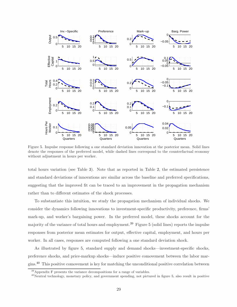
5 10 15 200
0.5
Out
put
Inv.−Specific
5 10 15 200
0.10.20.3
Preference
5 10 15 200
0.2
Mark−up
5 10 15 20
−0.05
0Barg. Power
5 10 15 200
1
Effe
ctiv
eC
apita
l
5 10 15 200
0.51
5 10 15 200
0.5
5 10 15 20−0.05
00.05
0.1
5 10 15 200
0.20.4
Tot
alH
ours
5 10 15 200
0.10.20.3
5 10 15 200
0.2
5 10 15 20
−0.1−0.05
0
5 10 15 200
0.2
Em
ploy
men
t
5 10 15 200
0.10.2
5 10 15 200
0.10.2
5 10 15 20
−0.1
0
5 10 15 200
0.1
Hou
rs P
erW
orke
r
Quarters5 10 15 20
00.020.040.060.08
Quarters5 10 15 20
0
0.05
Quarters5 10 15 20
0
0.02
0.04
Quarters
Figure 5. Impulse response following a one standard deviation innovation at the posterior mean. Solid linesdenote the responses of the preferred model, while dashed lines correspond to the counterfactual economywithout adjustment in hours per worker.
total hours variation (see Table 3). Note that as reported in Table 2, the estimated persistence
and standard deviations of innovations are similar across the baseline and preferred specifications,
suggesting that the improved fit can be traced to an improvement in the propagation mechanism
rather than to different estimates of the shock processes.
To substantiate this intuition, we study the propagation mechanism of individual shocks. We
consider the dynamics following innovations to investment-specific productivity, preference, firms’
mark-up, and worker’s bargaining power. In the preferred model, these shocks account for the
majority of the variance of total hours and employment.39 Figure 5 (solid lines) reports the impulse
responses from posterior mean estimates for output, effective capital, employment, and hours per
worker. In all cases, responses are computed following a one standard deviation shock.
As illustrated by figure 5, standard supply and demand shocks—investment-specific shocks,
preference shocks, and price-markup shocks—induce positive comovement between the labor mar-
gins.40 This positive comovement is key for matching the unconditional positive correlation between
39Appendix F presents the variance decompositions for a range of variables.40Neutral technology, monetary policy, and government spending, not pictured in figure 5, also result in positive
29

the labor margins. The main difference in propagation relative to the baseline model is that the low
wealth effect on the labor supply implies that hours per worker increase in response to positive sup-
ply and demand shocks, since hours per worker comove more tightly with the value of the marginal
product of hours.41 By contrast, labor-market shocks–shocks to workers’ bargaining power and
hours supply shocks—induce negative comovement. For instance, as displayed by the last column
of figure 5, an exogenous increase in workers’ bargaining power reduces employment—since workers
appropriate a larger share of the surplus through higher wages—and it increases hours per worker,
the relatively cheaper labor margin. The shock is recessionary as it increases the cost of production,
leading output, investment and consumption to decline.
The Role of Hours Supply Shocks
While parametrized wealth effects and hours adjustment costs are key ingredients for the model
to reproduce the empirical covariances of labor market variables, hours supply shocks remain an
important contributor for the variance of hours per worker— ht accounts for about 60 percent of the
volatility of ht. A natural question concerns the interpretation of hours supply shocks in the context
of the model. One possibility is that ht simply reflects measurement error. To rule this hypothesis,
we estimate an alternative version of the model that additionally allows for measurement error in
each observable. Even in this case, hours supply shocks still remain an important contributor to
fluctuations in hours per worker (results available upon request).
A closer look at the model equilibrium conditions presents a simple structural interpretation for
the role of ht at business cycle frequencies. Consider the log-linear approximation of the intratem-
poral condition for optimality in hours with the assumption that steady-state hours per worker are
normalized to one:
βt −1
Ψ
[CtC − hC
C
gA
(Ct−1 − gAt
)−
LX
1 + ω
(Lt + (1 + ω) ht + Xt
)]+ ht + Xt − uCt
= ϕt + α(uKt +
ˆKt − gAt − Lt − ht
)− φhht −
(ω +
XL
(1 + ω)Ψ
)ht,
where hats denote log-deviations. The right-hand side of this equation shows that ht acts as a time-
varying shifter of the marginal product of one hour worked, consistent with the empirical observation
that changes or differences in working hours do not entail the same changes or differences in effective
comovement in hours per worker and employment.41See Appendix E for a detailed comparison of impulse responses in the baseline and preferred model.
30

labor input (Pencavel, 2015). Thus, ht captures cyclical fluctuations in unobservable utilization of
hours per worker, reflecting variations in unobserved worker effort (see, for instance, Kimball et al.,
2006).42 In addition, ht captures exogenous fluctuations in the value of nonworking time, i.e., the
value of the opportunity cost of employment.43
6 Hours and Employment in Post-War U.S. Business Cycles
We now use the preferred model to empirically study the cyclical behavior of hours and employment
in U.S. data. We focus on U.S. business cycle recoveries—i.e., the progression of the economy after
having hit the trough of a recession—as there has been renewed interest in the topic in policy circles
(see Bernanke, 2003).
The impulse-response analysis discussed above rationalizes the observed time-varying comove-
ment between the margins of labor adjustment documented in section 2. When recoveries feature a
prominent role for standard supply and demand shocks, hours per worker and employment comove
positively. By contrast, when labor market shocks have a larger role, the adjustment along the two
margins displays a much lower correlation. The historical decompositions of employment and hours
per worker from the preferred model (presented in Appendix G) show that structural innovations
responsible for employment and hours per worker fluctuations in recoveries are consistent with these
comovements. For example, recessions and recoveries of 1970, 1975, and 1982 are predominantly
driven by investment-specific shocks, while those in 1991 and 2001 feature a more significant role
for labor-market shocks.44
Our model provides an ideal laboratory to quantify the contribution of the intensive margin
for employment outcomes. Towards this goal, we perform the following counterfactual. First,
we use the posterior mean estimates of the preferred model and the two-sided Kalman filter to
construct smoothed estimates of the structural shocks and model variables. We then construct a
counterfactual time series where hours are held constant at their steady-state value and compare
42Marchetti and Nucci (2014) document a hump-shaped profile of labor effort at business cycle frequencies. Noticethat ht may also capture in reduced-form other unmodeled features of hours adjustment such as overtime hours.A formal assesment of the quantitative importance of this alternative interpretation is precluded by the absence ofeconomy-wide data for overtime hours in the U.S. economy.
43The estimated preferred model is not only consistent with the labor margins emphasized in this paper, butalso with the properties of the opportunity cost of employment emphasized in Chodorow-Reich and Karabarbounis(2016). To demonstrate this, we use the observables and the two-sided Kalman filter at the posterior mean estimatesto generate smoothed, historical estimates of model variables, which by construction perfectly match employment andthe other macro observables to the data. The model-implies series generate 1) the opportunity cost of employment tobe more volatile than output and 2) procyclicality to the opportunity cost of employment, consistent with Chodorow-Reich and Karabarbounis (2016).
44The contribution of labor supply shocks in jobless recoveries is consistent with Aaronson et al. (2004).
31

the actual path to the hypothetical one where hours per worker are constant.45
Figure 6 contrasts the actual values of total hours, hours per worker, and employment (solid
lines) with the model counterfactual values (dashed lines).46 The figure shows that adjustment in
hours per worker has sizable effects on the recovery of total hours (up to 3.5 percentage points in
the recovery of 1982). The overall effect on total hours comes from both a direct and an indirect
effect. The direct effect accounts for the variation in total hours stemming from adjustments in
hours per worker for a given level of employment. The indirect effect accounts for the impact that
fluctuations in the intensive margin have on new matches (and thus employment) in response to
aggregate shocks. As shown by figure 6, lack of adjustment along the intensive margin would have
mitigated employment losses during recessions and resulted in quicker employment recoveries. We
find that the volatility of employment drops by 13 percent over the sample in the counterfactual
economy. Moreover, the standard deviation of total hours is 40 percent lower. Two-thirds of
this drop is accounted for by the lack of adjustment in hours-per-worker while the remaining part
depends on the indirect effect of the intensive margin on employment. These results imply that
hours adjustment contributes positively to employment volatility during post-war U.S. recessions
and recoveries.
What accounts for the importance of the indirect effect of hours per worker on employment?
Figure 7 plots the differences in the historical decompositions of employment from the preferred
and counterfactual models. As seen in the figure, investment-specific shocks account for most
of the differences in employment dynamics in the two economies. Labor market shocks also are
important.47
To understand the different transmission of these two shocks with and without the intensive-
margin adjustment, we return to our impulse response analysis. Figure 5 plots the responses
in the counterfactual economy with constant hours (dashed lines). An increase in investment-
specific productivity remains expansionary in the counterfactual economy. However, the absence of
hours adjustment implies a larger response of effective capital and a much lower response of total
hours. Since this shock induces positive comovement between the labor margins, the expected
present discounted value of new matches rises less in response to positive shocks when hours are
45Results are unaffected if hours per worker are held constant at the beginning of the trough of each recession(rather than at the beginning of the sample).
46Since total hours and employment are observables and there is no measurement error, the smoothed estimates ofthese variables from the two-sided Kalman filter, as well as hours per worker, perfectly match the data by construction.
47In particular, investment specific shocks account for large differences in the dynamics of the two economies in therecoveries of 1970, 1975 and 2001. Shocks to workers’ bargaining power are more important in the recovery of 1991,while the lack of hours supply shocks dominates in 1982.
32

−4 −2 0 2 4 6
0
2
4
Total Hours
197
0
−4 −2 0 2 4 60
0.5
1
1.5
Hours per Worker
197
0
−4 −2 0 2 4 6
−1
0
1
2
3
Employment
197
0
−4 −2 0 2 4 6
−6
−4
−2
0Total Hours
197
5
−4 −2 0 2 4 6
−1.5
−1
−0.5
0Hours per Worker
197
5
−4 −2 0 2 4 6−5
−4
−3
−2
−1
0Employment
197
5
−4 −2 0 2 4 6−8
−6
−4
−2
0Total Hours
198
2 −4 −2 0 2 4 6
−3
−2
−1
0Hours per Worker
198
2
−4 −2 0 2 4 6
−5
−4
−3
−2
−1
0Employment
198
2
−4 −2 0 2 4 6−2
−1
0
1
2
Total Hours
199
1
−4 −2 0 2 4 6
−1.5
−1
−0.5
0Hours per Worker
199
1
−4 −2 0 2 4 6
0
1
2
Employment
199
1
−4 −2 0 2 4 6−2
0
2
4
200
1
Total Hours
−4 −2 0 2 4 60
0.5
1
Hours per Worker
200
1
−4 −2 0 2 4 6
−2
0
2
Employment
200
1
Figure 6. U.S. recoveries relative to GDP trough. Blue solid lines: preferred model. Black dashed lines:counterfactual with hours per worker constant
2 4 6
−1
−0.5
0
0.5
Quarters
197
0
Employment
2 4 6
−1
−0.8
−0.6
−0.4
−0.2
0
0.2
197
5
Employment
Quarters2 4 6
−1.5
−1
−0.5
0
0.5
198
2
Employment
Quarters
2 4 6
−0.4
−0.2
0
0.2
0.4
0.6
Employment
199
1
Quarters2 4 6
−0.6
−0.4
−0.2
0
0.2
0.4Employment
200
1
Quarters
Technology
Preference
Inv Specific
Barg Power
Labor Supply
Markup
Govt Spending
Monetary
Initial Conditions
Figure 7. Differences between historical decompositions for employment in preferred model and counterfac-tual with hours per worker constant during U.S. recoveries.
33

constrained and do not increase. Moreover, achieving the same adjustment of total hours would
require additional vacancy posting in the counterfactual economy, which is costly due to congestion
externalities. All else equal, this decreases firms’ incentives to adjust employment, mitigating
employment’s response. Accordingly, firms raise effective capital more to meet a given demand.
Notice that, in general equilibrium, a second channel occurs through relative price adjustments.
Higher demand for effective capital raises the rental rate of capital, giving an incentive to producers
to substitute capital with labor (i.e., to hire more workers).48 In the case of an exogenous increase
in the workers’ bargaining power, firms can no longer substitute away from the relatively cheaper
labor input (hours per worker), leading employment to fall less than in the preferred model.
7 Sensitivity Analysis
We investigate the robustness of our results under several alternative specifications. The results
of these robustness checks are summarized in table 3. For reference, the first two rows report
the results of the baseline and preferred models, previously discussed. To understand how well
the model accounts for the labor market variables, we report for each specification the shares of
the variance of total hours attributed to hours per worker, employment, and their covariance. In
addition, we report log marginal data densities and twice the natural logarithm of Bayes factors
to provide an assessment of relative fit of models to the data, see section 5 for more discussion.
In all robustness cases, the preferred model implies a substantially greater fit. We discuss each
robustness case in turn.
The preferred model includes two additional features relative to the baseline, namely JR pref-
erences and costly hours adjustment. We consider each extension separately in the rows labeled
“Model w/o JR preferences” and “Model w/o costly hours adj.” Although each feature individually
improves the model’s fit relative to the baseline, the inclusion of both, the “Preferred Model” row,
provides the best fit. Omitting JR preferences reduces the model’s ability to match the positive
covariance between employment and hours per worker, as discussed in section 5.
48This feedback effect is stronger for shocks that are more persistent, since the present discounted value of jobcreation increases more in this case. In turn, the strength of the general equilibrium effect accounts for the responsesto preference and markup shocks in figure 5, as these shocks have high estimated persistence.
34

Alternative Shocks
We estimate the baseline model with seven observables when the hours supply shock is included as
opposed to the bargaining power shock. Hours supply shocks can potentially improve the model’s
fit with respect to labor market variables, as they directly affect the intensive labor margin. The
total hours variance shares in this case are listed in row “7 obs, h shock” of table 2. For comparison,
the estimates from the baseline model with seven observables is included for reference in row “7
obs, η shock.” While the hours supply shock does ensure the model matches the covariance of
employment and hours per worker, it does so with a counterfactually high volatility of hours per
worker, as βh’s bands encompass higher values than βL’s bands.
Wage Data
We document the robustness of our results to the wage observable. Using U.S. micro data, Haefke
et al. (2013) document that the wages of newly hired workers, unlike wages in ongoing relationships,
are volatile and procyclical. In addition, our baseline wage observable is not restricted to earnings,
as it includes employer contributions to employee-benefits (Justiniano et al., 2013). We address
these issues as follows. We estimate a version of the preferred model in which three measures of the
wage are simultaneously included in the observables. This strategy has been recently used by several
papers in the estimation literature (see for instance Boivin and Giannoni (2006), Gali et al. (2011),
and Justiniano et al. (2013)). The first is the measure described in section 4, which is the BLS’
hourly compensation for the nonfarm business sector. The second measure is the BLS’ average
Table 3: Robustness checks from Alternative Estimated Specifications.
Log Marginal 2 ln(Bayes Factor) βh βL βcov
Data Density vs. Preferred
CES Data 0.18 0.51 0.31
Preferred Model -1024 0 [0.13, 0.56] [0.20, 0.71] [-0.05, 0.44]Baseline Model -1073 98 [0.16, 0.76] [0.22, 0.89] [-0.43, 0.37]Model w/o JR preferences -1041 34 [0.13, 0.57] [0.24, 0.83] [-0.21, 0.41]Model w/o costly hours adj. -1043 38 [0.14, 0.58] [0.19, 0.57] [-0.04, 0.43]Preferred Model, mix wage obs -1332 0 [0.06, 0.56] [0.22, 0.95] [-0.28, 0.45]Baseline Model, mix wage obs -1380 96 [0.09, 0.72] [0.26, 1.12] [-0.62, 0.39]7 obs, η shock -1008 0 [0.03, 0.22] [0.64, 1.21] [-0.35, 0.25]7 obs, h shock -1076 136 [0.18, 0.60] [0.10, 0.50] [0.16, 0.44]
CPS Data 0.07 0.78 0.15
Preferred Model -1152 0 [0.05, 0.30] [0.31, 0.70] [0.14, 0.45]Baseline Model -1184 64 [0.11, 0.47] [0.26, 0.78] [-0.07, 0.43]
SW Data 0.39 0.44 0.17
Preferred Model -989 0 [0.14, 0.62] [0.18, 0.67] [-0.07, 0.42]Baseline Model -1051 124 [0.20, 0.83] [0.19, 0.80] [-0.40, 0.36]
Note: Parenthesis denote 90 percent posterior intervals. Log marginal data densities calculated using Geweke’s modifiedharmonic mean estimator; values are comparable conditional on observables, with different sets denoted by horizontal lines.
35

hourly earnings of production and nonsupervisory employees. The third measure is the quality
adjusted wage series of Haefke et al. (2013), which adjusts for individual-level characteristics. We
assume that each series represents an imperfect measure of the model wage according to:
Comp Waget
Earn Waget
Quality Waget
=
Γ1
Γ2
Γ3
(wt − wt−1 + gAt) +
e1t
e2t
e3t
where eit for i = 1, 2, 3 denote iid observation errors.49 Rows “Preferred Model, mix wage obs”
and “Baseline Model, mix wage obs” of Table 3 display the total hours variance shares in this case.
Again, the preferred model has a better fit, with bands well encompassing the data.
Alternative Labor Market Variables and Subsample Analysis
We check whether our results are sensitive to the labor market measures used for the estimation.
We estimate the model using CPS labor market variables, as in Ramey (2012).50 In this case,
neither total hours nor employment are linearly detrended as it is less obvious the series exhibit a
deterministic trend; the two variables are demeaned. Parameter estimates in this case are compara-
ble to those in table 2. Bayes factors suggest strong preference for the preferred model as well. As
shown in table 3, the posterior bands for the model’s βs well-encompass their data counterparts. In
addition, these results are robust to using the Smets and Wouters (2007) labor market observables
for estimation, which are commonly employed in the DSGE estimation literature, as evidenced by
the last rows of table 3.
Finally, our analysis of U.S. recoveries is robust to sub-sample estimation conditional on our
observables. This experiment allows us to address how structural change in parameter estimates (in
particular, those directly affecting labor market dynamics) contributes to the dynamics of hours and
employment in post-war U.S. data (the results are available upon request). As is common practice
in the literature, we split our original sample at the start of the so-called Great Moderation,
estimating from 1965:1 to 1983:4 and 1984:1 to 2007:4.
49The priors for the Γ’s are normal distributions centered at 1 with a standard deviation of 0.5. The priors for thestandard deviations of the wage observation errors are inverse gamma distributions with mean of 0.1 and standarddeviation of 1. Specifically, we use the median real wage of new hires corrected for fluctuations in all observable workercharacteristics from Haefke et al. (2013). This series is not available for the full sample period, but the Kalman filterhandles missing observations.
50See Appendix A for a description of the alternative labor market data.
36
8 Conclusions
We estimate a baseline search and matching model augmented with endogenous fluctuations in
hours per worker and shocks that affect both margins of labor adjustment. We show that this
baseline model is unable to replicate the correlation structure between aggregate macroeconomic
series and labor market variables. Two proposed modifications reconcile the model with the data:
adjustment costs to the intensive margin and a flexible parametrization of the strength of the short-
run wealth effect on hours supply, as first introduced by Jaimovich and Rebelo (2009). We use the
modified model to structurally assess the contribution of the intensive margin of labor adjustment
to aggregate dynamics.
We find the contribution of hours per worker to total hours is quantitatively significant, with a
notable component stemming from its indirect effect on employment adjustment. For instance, the
standard deviation of total hours is 40 percent lower in the constant hours counterfactual relative
to the estimated model. Two-thirds of this drop is accounted for by the lack of adjustment in
hours-per-worker while the remaining part depends on the indirect effect of the intensive margin
on employment.
While we estimate the model on U.S. data, our model introduces enough flexibility to allow the
model to match a broad array of empirical covariances between hours per worker and employment,
including potentially negative ones as observed in some European economies. Discerning the role
of the intensive margin for other countries, as well the introduction and study of country-specific
labor market policies, are important avenues for future research.
References
Aaronson, D., E. R. Rissman, and D. G. Sullivan (2004): “Assessing the Jobless Recovery,”Economic Perspectives, 2–21.
Altug, S., S. Kabaca, and M. Poyraz (2011): “Search Frictions, Financial Frictions andLabor Market Fluctuations in Emerging Economies,” Ko University-TUSIAD Economic ResearchForum Working Papers 1136, Koc University-TUSIAD Economic Research Forum.
Andolfatto, D. (1996): “Business Cycles and Labor-Market Search,” American Economic Re-
view, 86, 112–32.
Arseneau, D. M. and S. K. Chugh (2008): “Optimal Fiscal and Monetary Policy with CostlyWage Bargaining,” Journal of Monetary Economics, 55, 1401–1414.
——— (2012): “Tax Smoothing in Frictional Labor Markets,” Journal of Political Economy, 120,926–985.
37

Bachmann, R. (2012): “Understanding the Jobless Recoveries after 1991 and 2001,” Manuscript,University of Notre Dame.
Balleer, A., B. Gehrke, W. Lechthaler, and C. Merkl (2016): “Does Short-Time WorkSave Jobs? A Business Cycle Analysis,” European Economic Review, 84, 99–122.
Barro, R. J. (1977): “Long-Term Contracting, Sticky Prices, and Monetary Policy,” Journal of
Monetary Economics, 3, 305–316.
Beers, T. M. (2000): “Flexible Schedules and Shift Work: Replacing the ‘9-to-5’ Workday?”Monthly Labour Review, 33–40.
Bernanke, B. S. (2003): “The Jobless Recovery,” Remarks by Governor Ben S. Bernanke at the
Global Economic and Investment Outlook Conference, Carnegie Mellon University, PittsburghPennsylvania, November 6, 2003.
Boivin, J. and M. Giannoni (2006): “Has Monetary Policy Become More Effective?” Review of
Economics and Statistics, 88, 445–462.
Cahuc, P., F. Marque, and E. Wasmer (2008): “A Theory of Wages and Labor Demand WithIntra-Firm Bargaining and Matching Frictions,” International Economic Review, 49, 943–972.
Campolmi, A. and S. Gnocchi (2016): “Labor Market Participation, Unemployment and Mon-etary Policy,” Journal of Monetary Economics, 79, 17 – 29.
Cho, J.-O. and T. F. Cooley (1994): “Employment and Hours over the Business Cycle,” Journal
of Economic Dynamics and Control, 18, 411–432.
Chodorow-Reich, G. and L. Karabarbounis (2016): “The Cyclicality of the OpportunityCost of Employment,” Journal of Political Economy, 124, 1563–1618.
Christiano, L. J., M. Eichenbaum, and C. L. Evans (2005): “Nominal Rigidities and theDynamic Effects of a Shock to Monetary Policy,” Journal of Political Economy, 113, 1–45.
Christiano, L. J., M. S. Eichenbaum, and M. Trabandt (2016): “Unemployment and Busi-ness Cycles,” Econometrica, 84, 1523–1569.
Christiano, L. J. and T. J. Fitzgerald (2003): “The Band Pass Filter*,” International Eco-
nomic Review, 44, 435–465.
Christiano, L. J., M. Trabandt, and K. Walentin (2011): “Introducing Financial Frictionsand Unemployment into a Small Open Economy Model,” Journal of Economic Dynamics and
Control, 35, 1999–2041.
Davis, S. J., J. C. Haltiwanger, and S. Schuh (1998): Job Creation and Destruction, vol. 1of MIT Press Books, The MIT Press.
Del Negro, M., F. Schorfheide, F. Smets, and R. Wouters (2007): “On the Fit of NewKeynesian Models,” Journal of Business & Economic Statistics, 25, 123–143.
den Haan, W. J., G. Ramey, and J. Watson (2000): “Job Destruction and Propagation ofShocks,” American Economic Review, 90, 482–498.
38
Francis, N. and V. A. Ramey (2009): “Measures of per Capita Hours and Their Implicationsfor the Technology-Hours Debate,” Journal of Money, Credit and Banking, 41, 1071–1097.
Frazis, H. and J. Stewart (2010): “Why Do BLS Hours Series Tell Different Stories AboutTrends in Hours Worked?” in Labor in the New Economy, ed. by K. G. Abraham, J. R. Spletzer,and M. Harper, Princeton, NJ: University of Chicago Press, 343–372.
Fujita, S. and G. Ramey (2009): “The Cyclicality Of Separation and Job Finding Rates,”International Economic Review, 50, 415–430.
Gali, J., F. Smets, and R. Wouters (2011): “Unemployment in an Estimated New KeynesianModel,” NBER Macroeconomics Annual, 26, 329–360.
——— (2012): “Slow Recoveries: A Structural Interpretation,” Journal of Money, Credit and
Banking, 44, 9–30.
Gertler, M., L. Sala, and A. Trigari (2008): “An Estimated Monetary DSGE Model withUnemployment and Staggered Nominal Wage Bargaining,” Journal of Money, Credit and Bank-
ing, 40, 1713–1764.
Gertler, M. and A. Trigari (2009): “Unemployment Fluctuations with Staggered Nash WageBargaining,” Journal of Political Economy, 117, 38–86.
Geweke, J. (1999): “Using Simulation Methods for Bayesian Econometric Models: Inference,Development, and Communication,” Econometric Reviews, 18, 1–73.
Greenwood, J., Z. Hercowitz, and G. W. Huffman (1988): “Investment, Capacity Utiliza-tion, and the Real Business Cycle,” American Economic Review, 78, 402–17.
Groshen, E. L. and S. M. Potter (2003): “Has Structural Change Contributed to a JoblessRecovery?” Current Issues in Economics and Finance, 9.
Haefke, C., M. Sonntag, and T. Van Rens (2013): “Wage Rigidity and Job Creation,” Journal
of Monetary Economics, 60, 887–899.
Hall, R. E. (2005): “Employment Fluctuations with Equilibrium Wage Stickiness,” American
Economic Review, 95, 50–65.
Hansen, G. D. and T. J. Sargent (1988): “Straight Time and Overtime in Equilibrium,”Journal of Monetary Economics, 21, 281–308.
Hirose, Y. and A. Inoue (2015): “The Zero Lower Bound and Parameter Bias in an EstimatedDSGE Model,” Journal of Applied Econometrics, forthcoming.
Imbens, G. W., D. B. Rubin, and B. Sacerdote (1999): “Estimating the Effect of UnearnedIncome on Labor Supply, Earnings, Savings, and Consumption: Evidence from a Survey ofLottery Players,” NBER Working Papers.
Jaimovich, N. and S. Rebelo (2009): “Can News about the Future Drive the Business Cycle?”American Economic Review, 99, 1097–1118.
Jaimovich, N. and H. E. Siu (2012): “The Trend is the Cycle: Job Polarization and JoblessRecoveries,” NBER Working Papers 18334, National Bureau of Economic Research, Inc.
39

Justiniano, A. and C. Michelacci (2012): “The Cyclical Behavior of Equilibrium Unem-ployment and Vacancies in the United States and Europe,” NBER International Seminar on
Macroeconomics, 8, 169 – 235.
Justiniano, A., G. E. Primiceri, and A. Tambalotti (2010): “Investment Shocks and Busi-ness Cycles,” Journal of Monetary Economics, 57, 132–145.
——— (2013): “Is There a Trade-Off between Inflation and Output Stabilization?” American
Economic Journal: Macroeconomics, 5, 1–31.
Kass, R. E. and A. E. Raftery (1995): “Bayes Factors,” Journal of the American Statistical
Association, 90, 773–795.
Kimball, M. S., J. G. Fernald, and S. Basu (2006): “Are Technology Improvements Con-tractionary?” American Economic Review, 96, 1418–1448.
Kirkland, K. (2000): “On the Decline in Average Weekly Hours Worked,” Monthly Labour
Review, 26–31.
Kydland, F. E. and E. C. Prescott (1991): “Hours and Employment Variation in BusinessCycle Theory,” Economic Theory, 1, 63–81.
Marchetti, D. J. and F. Nucci (2014): Wealth, Income Inequalities, and Demography: The
Long-Term Policy View, Cham: Springer International Publishing, chap. Effort and Hours overthe Business Cycle, 229–249.
Merz, M. (1995): “Search in the Labor Market and the Real Business Cycle,” Journal of Monetary
Economics, 36, 269–300.
Merz, M. and E. Yashiv (2007): “Labor and the Market Value of the Firm,” American Economic
Review, 97, 1419–1431.
Mortensen, D. T. and C. A. Pissarides (1994): “Job Creation and Job Destruction in theTheory of Unemployment,” Review of Economic Studies, 61, 397–415.
Ohanian, L. E. and A. Raffo (2012): “Aggregate Hours Worked in OECD Countries: NewMeasurement and Implications for Business Cycles,” Journal of Monetary Economics, 59, 40–56.
Pencavel, J. (2015): “The Productivity of Working Hours,” The Economic Journal, 125, 2052–2076.
Petrongolo, B. and C. Pissarides (2006): “Scale Effects in Markets with Search,” Economic
Journal, 116, 21–44.
Pissarides, C. A. (2000): Equilibrium Unemployment Theory, 2nd Edition, vol. 1 of MIT Press
Books, The MIT Press.
Ramey, V. A. (2012): “The Impact of Hours Measures on the Trend and Cycle Behavior of U.S.Labor Productivity,” Manuscript, University of California–San Diego.
Ravenna, F. and C. E. Walsh (2011): “Welfare-Based Optimal Monetary Policy with Un-employment and Sticky Prices: A Linear-Quadratic Framework,” American Economic Journal:
Macroeconomics, 3, 130–62.
40

——— (2012): “Screening and Labor Market Flows in a Model with Heterogeneous Workers,”Journal of Money, Credit and Banking, 44, 31–71.
Ravn, M. O. and S. Simonelli (2007): “Labor Market Dynamics and the Business Cycle:Structural Evidence of the United States,” Scandinavian Journal of Economics, 109, 743–777.
Rotemberg, J. J. (1982): “Monopolistic Price Adjustment and Aggregate Output,” Review of
Economic Studies, 49, 517–31.
Schmitt-Grohe, S. and M. Uribe (2007): “Optimal Simple and Implementable Monetary andFiscal Rules,” Journal of Monetary Economics, 54, 1702–1725.
Schreft, S. L., A. Singh, and A. Hodgson (2005): “Jobless Recoveries and the Wait-and-SeeHypothesis,” Economic Review, 81–99.
Shimer, R. (2005): “The Cyclical Behavior of Equilibrium Unemployment and Vacancies,” Amer-
ican Economic Review, 95, 25–49.
Smets, F. and R. Wouters (2007): “Shocks and Frictions in US Business Cycles: A BayesianDSGE Approach,” American Economic Review, 97, 586–606.
Thomas, C. (2008): “Search and Matching Frictions and Optimal Monetary Policy,” Journal of
Monetary Economics, 55, 936–956.
Trigari, A. (2009): “Equilibrium Unemployment, Job Flows, and Inflation Dynamics,” Journal
of Money, Credit and Banking, 41, 1–33.
Wolters, M. H. (2016): “How the Baby Boomers’ Retirement Wave Distorts Model-Based Out-put Gap Estimates,” Kiel Working Papers No. 2031.
Woodford, M. (2003): “Interest and Prices: Foundations of a Theory of Monetary Policy,”Princeton University Press.
41


![Alfie Kohn - Unconditional Parenting[1]](https://static.fdocuments.in/doc/165x107/577cc60c1a28aba7119d900b/alfie-kohn-unconditional-parenting1.jpg)