Houghton, C., & Lee, K. (1999). Nahm Data and the Mass of 1/4-BPS States.Phys.Rev. E. 10.1103/PhysRevD.61.106001

Link to published version (if available):10.1103/PhysRevD.61.106001

Link to publication record in Explore Bristol ResearchPDF-document

University of Bristol - Explore Bristol ResearchGeneral rights

This document is made available in accordance with publisher policies. Please cite only the publishedversion using the reference above. Full terms of use are available:http://www.bristol.ac.uk/pure/about/ebr-terms.html

Take down policy

Explore Bristol Research is a digital archive and the intention is that deposited content should not beremoved. However, if you believe that this version of the work breaches copyright law please contactopen-access@bristol.ac.uk and include the following information in your message:

• Your contact details• Bibliographic details for the item, including a URL• An outline of the nature of the complaint

On receipt of your message the Open Access Team will immediately investigate your claim, make aninitial judgement of the validity of the claim and, where appropriate, withdraw the item in questionfrom public view.

brought to you by COREView metadata, citation and similar papers at core.ac.uk

provided by Explore Bristol Research

arX

iv:h

ep-t

h/99

0921

8v2

31

Mar

200

0

DAMTP-1999-104SNUTP-99-042

KIAS-P99089

hep-th/9909218

Nahm Data and the Mass of 1/4-BPS States

Conor J. Houghton,∗

DAMTP, University of Cambridge, Silver St., Cambridge, CB3 9EW, UK.

and

Physics Department, Columbia University, New York, New York 10027, USA.†

Kimyeong Lee,‡

Physics Department and Center for Theoretical Physics,

Seoul National University, Seoul 151-742, Korea.

and

School of Physic, Korea Institute for Advanced Study

207-43, Cheongryangryi-Dong, Dongdaemun-Gu, Seoul 130-012, Korea.§

September 29, 1999

Abstract

The mass of 1/4-BPS dyonic configurations in N = 4 D = 4 supersymmetricYang-Mills theories is calculated within the Nahm formulation. The SU(3) example,with two massive monopoles and one massless monopole, is considered in detail. Inthis case, the massless monopole is attracted to the massive monopoles by a linearpotential.

∗E-mail: houghton@cuphyb.phys.columbia.edu†Address during academic year 1999/2000‡E-mail: kimyeong@phya.snu.ac.kr§Address from September 1, 1999

1

1 Introduction

In the context of N = 4 supersymmetric Yang-Mills theories in four-dimensionalspacetime, BPS magnetic monopoles are referred to as 1/2-BPS states, because they areinvariant under half of the supersymmetry. Recently, 1/4-BPS states have also been con-sidered. 1/4-BPS states are invariant under only a quarter of the supersymmetry and formsomewhat larger supermultiplets.

Generally, there are six scalar fields in N = 4 supersymmetric Yang-Mills theory. Fora configuration to be 1/4 BPS, all but two of these scalar fields must vanish and theremaining two must satisfy two field equations called BPS equations. The first of theseequations requires that the gauge fields Ai and one of the scalar fields, b, must satisfy theusual Bogomolny equation for BPS monopoles. The second BPS equation requires thatthe other scalar field, a, must satisfy the covariant Laplace equation in the background ofthe solution, Ai and b, of the first BPS equation.

A point in the moduli space of 1/2-BPS configurations corresponds to a unique 1/4-BPS configuration; the field a is determined uniquely. This means the contribution ofa to the mass of the 1/4-BPS state is a potential function over the moduli space. Thecontribution of a to the mass is referred to as the electric part of the mass, or simply,the electric mass. It is thought that there may be a moduli space approximation to thelow energy dynamics of 1/4-BPS states with kinetic term given by the usual moduli spacemetric and with potential term given by half the electric mass.

It is difficult to solve the two BPS equations. The most tractable approach is to employthe Nahm formulation. Using the Nahm formulation, the fields were found for a simple casein [1]. Another approach is to study spherically symmetric solutions and use a sphericalansatz to solve the field equations [2, 3].

However, past experience has shown that a great deal can be learned about 1/2-BPSconfigurations, without knowing the explicit fields. It appears that this is also the casewith 1/4-BPS configurations. The solutions of the first BPS equations are described bymoduli space coordinates and there is a natural metric on the moduli space. In a numberof examples, this metric is known even though the fields are not. Furthermore, the electriccharge and the electric part of the BPS energy can be obtained from the moduli spacemetric without solving the BPS equations for the fields [4].

In this paper, we show that the electric mass may also be calculated directly from theNahm data, without having to calculate either the fields or the metric. We apply this totwo SU(3) examples. In the first example, b is a (1, 1)-monopole. In this case, the electricmass is already know from more direct calculations [1, 4]. In the second example, the bfield is the (2, [1])-monopole considered by Dancer [5, 6]. The electric mass has not beenpreviously calculated for this case and, so, it is discussed in some detail.

A (2, [1])-monopole is a monopole in the theory with SU(3) symmetry broken to U(2)by the asymptotic value of b. In other words, SU(3) has two simple roots, α and β, andthe asymptotic value of b is perpendicular to β, permitting a U(2) of gauge inequivalentlarge gauge transformations of the fields. This means that the theory has two types ofmonopoles: massive α monopoles and massless β monopoles. The nonabelian case is

2

usefully thought of as a limit of the generic case, where the asymptotic value of b is notperpendicular to either root [7].

A (2, [1])-monopole is composed of two α monopoles and one β monopole. The modulispace of (2, [1])-monopoles describes the solutions of the first BPS equation. The netmagnetic charge is purely abelian and the massless β monopole forms a nonabelian cloudsurrounding the two massive α monopoles. However, this discussion refers only to thecontribution that b makes to the mass. The asymptotic value of the second Higgs field, a,breaks the symmetry further to U(1)×U(1). This symmetry breaking pattern is requiredfor genuine 1/4-BPS configurations. When the asymptotic values of the two Higgs fieldsare proportional, the Higgs fields are proportional everywhere. This means that there isreally only one active scalar field and the configuration is 1/2 BPS. In a genuine 1/4-BPSconfiguration, the β monopole is not massless if the contribution of the a field is included.

A similar situation arose in the (1, [1], 1) case recently considered by one of us (KL) [8].Here, the SU(4) symmetry is broken to U(1) × SU(2) × U(1) by the b field and is brokenmaximally by the a field. Due to the recent progress in the understanding of 1/4-BPSconfigurations, some remarks can now be made about the (2, [1]) case which also apply tothe (1, [1], 1) case. It is emphasized that the precise position of the massless β monopole isimportant in the 1/4-BPS configuration. As far as the field b is concerned, the position ofthe massless monopole can be transformed by the unbroken symmetry. In fact, if a masslessmonopole is considered as the massless limit; then some of the moduli of the monopolebecome, in the limit, parameters of the orbit of the unbroken symmetry. On the otherhand, the asymptotic a field breaks the SU(2) symmetry and so the solution depends onthe position of the massless monopole. Similarly, if there were several identical masslessmonopoles, the solution of the second BPS equation would depend on the moduli of themassless monopoles.

Recently, a low energy effective lagrangian for the moduli dynamics of 1/4-BPS config-urations has been found [9]. It consists of a kinetic part and a potential part. The kineticpart is given by the moduli space metric of the corresponding 1/2-BPS monopole. Thepotential part is given by half of the electric mass. The non-relativistic lagrangian has aBPS bound, and the BPS configuration saturating this bound turns out to be the 1/4-BPSfield theoretic configuration. Naive criteria, for specifying the valid region of this low en-ergy lagrangian, require that the kinetic energy and the potential energy are much smallerthan the rest mass of the monopoles involved. When massless monopoles are involved, itis not clear whether there is any valid region. However, if such a region exists, it wouldhave to be one where the energy is smaller than the magnetic mass of the configuration.In this paper, we assume that a valid region exists and we explore the consequences. Thepicture which emerges appears to be consistent.

The potential in the (2, [1]) case is quite interesting. It is repulsive and the relativeelectric charge between dyons generates an effective attractive force. There is a minimumallowed electric charge, which matches nicely with the string picture. The balance of theattractive electric force and the repulsive force leads to the BPS configurations. Moreover,when we try to remove the apparently massless β monopole away from the α monopoles,it turns out that the potential grows linearly with distance from the two α monopoles to

3

the β monopole. This is a sort of confinement. Of course, it would be strange if we couldtake out the massless monopole with a finite energy cost since it would then appear to beboth massive and massless.

In section 2, there is a review of the physics of 1/4-BPS configurations. In section 3,we discuss 1/4-BPS configurations in the Nahm formulation and derive a formula for theelectric mass. This formula is used to calculate the known electric mass potential in the(1, 1) case. In section 4, the formula is used to calculate the mass of 1/4-BPS states inthe (2, [1]) case. A string configuration equivalent to this state is proposed. Finally, weconclude with some remarks in section 5.

2 1/4-BPS configurations

A N = 4 supersymmetric Yang-Mills theory has a six component scalar field. Four ofthese components are zero in 1/4-BPS configurations [1] and it is possible to choose twoindependent orthogonal Higgs fields a and b satisfying

Bi = Dib (2.1)

andDiDia + [b, [b, a]] = 0 (2.2)

where the coupling constant, e, is set to one. In this context, these are referred to asthe first and second BPS equations. The gauge group is SU(N). Thus, Ai and b satisfythe usual Bogomolny equation for 1/2-BPS monopoles and a satisfies a covariant Laplaceequation in the background of Ai and b. The equation satisfied by a is the same as theequation satisfied by a large gauge transformation of Ai and b obeying the backgroundgauge condition. The appearance of the Bogomolny equation apparently reflects the factthat some of the supersymmetry is unbroken. There is no Bogomolny equation in thenon-BPS case, where three of the scalar fields are active [3].

A general configuration has both magnetic and electric charges. Asymptotically, theHiggs field lies in the gauge orbit of

b ≃ b · H − 1

4πrg · H, (2.3)

a ≃ a · H− 1

4πrq ·H, (2.4)

where the dot product of bold quantities is in the Cartan space. The mass of the corre-sponding configuration is

b · g + a · q (2.5)

Thus, there are two contributions to the mass: b · g and a ·q. These are referred to as themagnetic mass and the electric mass respectively.

The solutions of the first BPS equation, (2.1), are 1/2-BPS monopoles. Generally, theasymptotic value, b, of b breaks SU(N) to U(1)N−1 and there exists a unique set of simple

4

roots β1, β2, . . . , βN−1 such that βI ·b > 0 for I = 1 . . . N − 1. For each simple root, thereis a fundamental monopole with four zero modes. For any magnetic charge

g = g(k1β1 + k2β2 + ... + kN−1βN−1) (2.6)

with non-negative kI , there exists a family of 1/2-BPS solutions of the first BPS equation,called (k1, k2, . . . , kN−1)-monopoles [10]. Usually g = 4π. The solutions are uniquely char-acterized by their moduli space coordinates. Thus, any specific solution of the first BPSequation is given by the coordinates zp of the moduli space of these 1/2-BPS monopoles.The dimension of the moduli space is 4× (k1 + k2 + ...+ kN−1) and there exists a naturallydefined metric on this moduli space, given by the L2 norm of gauge-orthogonal field vari-ations. The magnetic mass is the same for all monopoles with the same magnetic chargeand is given by

b · g = g∑

I

kIµI (2.7)

where gµI is the mass of the Ith type of monopole.The symmetry breaking is not maximal when βI ·b = 0 for some I. The corresponding

fundamental monopole becomes massless and does not exist in isolation. However, whenthe total magnetic charge g is purely abelian, so that g · βI = 0 for βI · b = 0, thereare massless monopoles with kI = (kI+1 + kI−1)/2. These massless monopoles appear as anonabelian cloud surrounding the massive monopoles. As long as the total magnetic chargeremains purely abelian the dimension of the moduli space does not change in the masslesslimit [10, 7]. However, the meaning of the moduli space coordinate changes from the pointof view of 1/2-BPS configurations. The position and phase of massless monopoles becomethe unbroken nonabelian gauge orbit parameters and gauge invariant cloud parameters.

A solution of the second BPS equation can be found for each solution of the first BPSequation. In fact, the second BPS equation is identical to the zero mode equation forgauge-orthogonal large gauge transformations of the fields. There are N − 1 such zeromodes since SU(N) breaks into N − 1 abelian U(1) groups. From the solution of thesecond BPS equations, the electric charges carried by the kI βI monopoles can be read offfrom the asymptotic field (2.4).

Thus, when the asymptotic value, b, leaves some of the nonabelian gauge symmetryunbroken, the 1/2-BPS configurations may involve massless monopoles. The asymptoticvalue a may preserve the unbroken symmetry by b or break it further. When there isan unbroken nonabelian symmetry group, there may be non-vanishing, nonabelian electriccharge for a 1/4-BPS configurations. This is shown in a simple case in [8].

3 The Nahm formulation

In this section, we first review the Nahm formulation for the first BPS equation.We then derive a formula for the electric mass using the Nahm formulation. There is acomplication when two adjacent charges are equal, as in the (1, 1) case. In subsection 3.1,

5

we extend our formula to these cases. The specific example of the (1, 1) case is consideredin subsection 3.2. In the next section, the formula is applied to the (2, [1]) case.

BPS monopoles are classified by Nahm data [11, 12]. Nahm data are a 4-vector ofskewhermetian matrix functions of one variable over the subdivided interval defined by theeigenvalues of the asymptotic Higgs field b · H. Inside each subinterval, the data satisfythe Nahm equation

dTi

ds+ [T0, Ti] = [Tj , Tk] (3.1)

where (i j k) is a cyclic permutation of (1 2 3). Each subinterval corresponds to one of theunbroken U(1) subgroups of SU(N) and the magnetic charge around that U(1) determinesthe size of the Nahm matrices over that subinterval. Thus, a (k1, k2, . . . , kN−1)-monopolewith Higgs field at spatial infinity is given by

b ·H = −idiag(s1, s2, . . . , sN) (3.2)

where s1 < s2 < . . . < sN , corresponds to Nahm data over the interval (s1, sN). Over(s1, s2), the Nahm matrices are k1 ×k1, over (s2, s3) they are k2 ×k2 and so on. It is usefulto illustrate Nahm data with a graph, taking the value kI over the Ith interval.

Boundary conditions relate the Nahm matrices in abutting subintervals. For

6

?

k1

s0

k2

6

?

(3.3)

the Nahm matrices are k1 × k1 matrices if s < s0 and k2 × k2 matrices if s > s0. Theboundary condition requires that

Ti(s0−) = blockdiag (Ri/(s − s0), Ti(s0+)) (3.4)

where the (k1 − k2) × (k1 − k2) residue matrices Ri must form the (k1 − k2)-dimensionalirreducible representation of su(2). Thus, part of the data carries through the junction andthe rest has a pole with residues of a particular type.

The boundary conditions are different when k1 = k2. In this case the data carryingthough may have a rank one discontinuity. Thus, for

6

?k

s0

(3.5)

the boundary condition at s = s0 is

∆Ti = Ti(s0+) − Ti(s0−) =i

2trace2 σiww† (3.6)

6

where w is a 2 × k matrix, ww† is a tensor product over both indices and trace2 (·) sumsthe diagonal of the 2× 2 part of the product. w is often called the jump or matching data.The boundary condition is sometimes included in the Nahm equation as a source term

dTi

ds+ [T0, Ti] = [Tj , Tk] +

i

2trace2 σiww†δ(s − s0). (3.7)

This practice is not adopted here.The boundary conditions for non-maximal symmetry breaking can be derived from

those above by identifying eigenvalues.There is a group action on Nahm data given by

T0 → GT0G−1 − dG

dsG−1,

Ti → GTiG−1 (3.8)

where G is a group valued function of s. For this to act on Nahm data, G must satisfycertain boundary conditions on the subintervals. Depending on how strong the boundaryconditions satisfied are, G is a large or small gauge transformation. The moduli spaceof Nahm data is defined relative to small gauge transformations. The precise form ofboundary conditions on the group transformations and the criterion distinguishing largeand small gauge transformations of the Nahm data are discussed for specific examples in[5, 13].

In [1], the Nahm formulation of 1/4-BPS states is derived by applying the Fourieranalysis methods of [14] to the ADHM formulation of the Laplace equation for an instantonbackground [15]. By partially performing the ADHMN construction a · q is calculated for(1, 1)-monopoles. A technique is now presented which simplifies the calculation of the massin the Nahm formulation. This technique relies on the isometry between the space of Nahmdata and the moduli space of monopoles. In fact, while it is believed that these spaces areisomorphic in general, this has only been proven in specific cases [16].

In [4], an expression is derived for the mass of a 1/4-BPS state as a function over themonopole moduli space. The argument that is used there is reversed to allow us to writethe mass in terms of the solution to the covariant Laplace equation on Nahm data. Theelectric contribution to the mass is

a · q = trace

∫

d3x∑

i

∂i(aDia)

= trace

∫

d3x{∑

i

(Dia)2 − [a, b]2}. (3.9)

In [4], it is noted that Dia is a large gauge transformation in Ai and can be written as

Dia =∑

p

a ·KpδpAi. (3.10)

7

In the same way,

− i[b, a] =∑

p

a · Kpδpb (3.11)

where δpAi and δpb are the zero modes for the 1/2-BPS configurations and Kp are theKilling vectors for the large gauge transformations. Substituting these expressions into(3.9) and using the equation satisfied by a gives the Tong formula

a · q =∑

p,q

gpq(a · Kp)(a ·Kq) (3.12)

where

gpq(z) = trace

∫

d3x

(

∑

i

δpAiδqAi + δpb δqb

)

. (3.13)

This formula allows the electric mass to be calculated from the metric; it does not requirethat the fields are known.

The metric can also be written in terms of Nahm data:

gpq = −gtrace

∫

ds∑

µ

δpTµδqTµ. (3.14)

This expression can be substituted into the Tong formula (3.12) and the derivation can bereversed to give a formula for a · q in terms of a large gauge transformation of the Nahmdata satisfying the background gauge condition. There is a factor of g in (3.14 because themass of a static monopole is gµ rather than µ.

An infinitesimal gauge transformation h of the Nahm data is given by

δT0 = −dh

ds− [T0, h],

δTi = −[Ti, h] (3.15)

and the background gauge condition is

dδT0

ds+∑

µ

[Tµ, δTµ] = 0. (3.16)

This is derived by requiring that variations are orthogonal to small gauge transformationsof the data. Thus, a gauge-orthogonal large gauge transformation, p, satisfies the covariantLaplace equation

[d

ds+ T0, [

d

ds+ T0, p]] +

∑

i

[Ti, [Ti, p] = 0. (3.17)

This is the equation discussed in [1]: the only differences result from the convention ofusing skewhermetian rather than hermetian Nahm data.

8

Now, substituting

∑

p

a · KpδpT0 = −dp

ds− [T0, p],

∑

p

a · KpδpTi = −[Ti, p] (3.18)

into (3.14) and using the covariant Laplace equation (3.17) gives

a · q = −gtrace

∫

dsd

ds

[

p

(

dp

ds+ [T0, p]

)]

= −gtrace

∫

dsd

ds

(

pdp

ds

)

. (3.19)

This is the formula for the mass in terms of the 1/4-BPS Nahm data. It allows the ADHMNconstruction to be avoided when calculating the mass.

A difficulty with using this formula is calculating what a is. In the example consideredin section 4, this is not difficult as the form of the group action on the Nahm is very clear.It is more difficult in more trivial examples, where p is proportional to the identity. In thesecases it seems the ADHMN construction must be examined. The ADHMN constructionfor 1/4-BPS states is described in [1]. In short, a linear equation, known as the ADHMNequation, is solved for a set of N complex vector functions vI(s; x1, x2, x3). b and a arethen given by

bIJ =

∫

isv†IvJds

aIJ =

∫

v†I(p ⊗ 12)vJds. (3.20)

There is a tensor product with 12 in the formula for a. This matches the tensor productin the ADHMN equation.

Let us consider the trivial SU(2) example. In the SU(2) case, b is a k-monopole andthere is no genuine 1/4-BPS state, since the only solution to the second BPS equationhas a proportional to b. The only non-singular solution to the covariant Laplace equation(3.17) is

p = Ais1k (3.21)

where A is a constant. By (3.20) this means

a = Ab. (3.22)

Thus a = Ab, q = Aa and the electric mass can be calculated both directly and by usingthe formula (3.19). Either way

a · q = A2gkµ = A2b · g. (3.23)

9

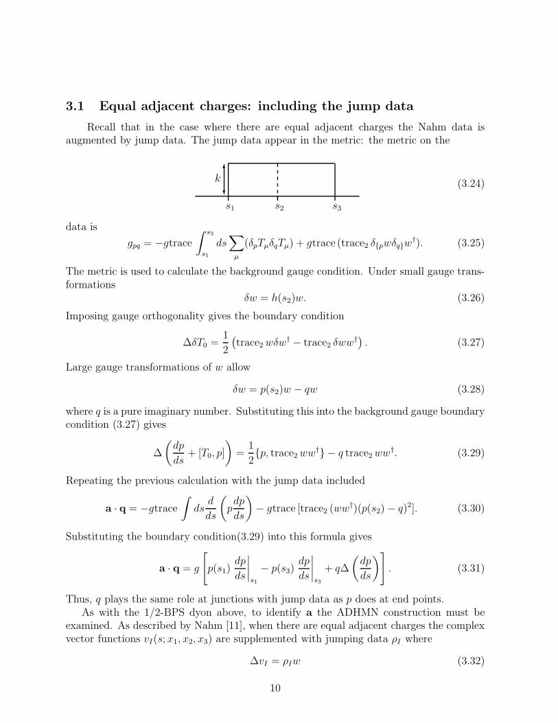
3.1 Equal adjacent charges: including the jump data

Recall that in the case where there are equal adjacent charges the Nahm data isaugmented by jump data. The jump data appear in the metric: the metric on the

6

?k

s1 s2 s3

(3.24)

data is

gpq = −gtrace

∫ s3

s1

ds∑

µ

(δpTµδqTµ) + gtrace (trace2 δ{pwδq}w†). (3.25)

The metric is used to calculate the background gauge condition. Under small gauge trans-formations

δw = h(s2)w. (3.26)

Imposing gauge orthogonality gives the boundary condition

∆δT0 =1

2

(

trace2 wδw† − trace2 δww†)

. (3.27)

Large gauge transformations of w allow

δw = p(s2)w − qw (3.28)

where q is a pure imaginary number. Substituting this into the background gauge boundarycondition (3.27) gives

∆

(

dp

ds+ [T0, p]

)

=1

2{p, trace2 ww†} − q trace2 ww†. (3.29)

Repeating the previous calculation with the jump data included

a · q = −gtrace

∫

dsd

ds

(

pdp

ds

)

− gtrace [trace2 (ww†)(p(s2) − q)2]. (3.30)

Substituting the boundary condition(3.29) into this formula gives

a · q = g

[

p(s1)dp

ds

∣

∣

∣

∣

s1

− p(s3)dp

ds

∣

∣

∣

∣

s3

+ q∆

(

dp

ds

)

]

. (3.31)

Thus, q plays the same role at junctions with jump data as p does at end points.As with the 1/2-BPS dyon above, to identify a the ADHMN construction must be

examined. As described by Nahm [11], when there are equal adjacent charges the complexvector functions vI(s; x1, x2, x3) are supplemented with jumping data ρI where

∆vI = ρIw (3.32)

10

and

bIJ = is2ρ⋆IρJ +

∫ s3

s1

isv†IvJds. (3.33)

Standard arguments involving approximate solutions of the ADHMN equation are thenused to prove [11, 12] that

b · H = −i

s1

s2

s3

(3.34)

In the 1/4-BPS case [1],

aIJ = qρ⋆IρJ +

∫ s3

s1

v†I(p ⊗ 12)vJds. (3.35)

If p ∝ 1k, then the same standard arguments prove that

a · H = −

p(s1)q

p(s3)

. (3.36)

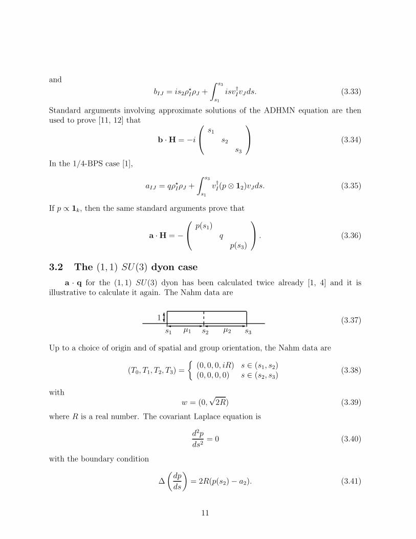
3.2 The (1, 1) SU(3) dyon case

a · q for the (1, 1) SU(3) dyon has been calculated twice already [1, 4] and it isillustrative to calculate it again. The Nahm data are

6?1

s1 s2 s3µ2µ1

-�-� (3.37)

Up to a choice of origin and of spatial and group orientation, the Nahm data are

(T0, T1, T2, T3) =

{

(0, 0, 0, iR) s ∈ (s1, s2)(0, 0, 0, 0) s ∈ (s2, s3)

(3.38)

withw = (0,

√2R) (3.39)

where R is a real number. The covariant Laplace equation is

d2p

ds2= 0 (3.40)

with the boundary condition

∆

(

dp

ds

)

= 2R(p(s2) − a2). (3.41)

11

The solution is

p =

{

ip1(s − s1) + ia1 s ∈ (s1, s2)ip2(s − s3) + ia3 s ∈ (s2, s3)

(3.42)

where the boundary conditions imply

p1µ1 + a1 = −p2µ2 + a3

= a2 +1

2R(p2 − p1) (3.43)

and q = ia3. Solving for p1 and p2 gives

p1 =a3 − a1 + 2(a2 − a1)µ2R

µ1 + µ2 + 2µ1µ2R,

p2 =a1 − a3 + 2(a2 − a3)µ1R

µ1 + µ2 + 2µ1µ2R(3.44)

and the electric mass formula (3.31) gives

a · q = g(a2 − a1)p1 + g(a3 − a2)p2. (3.45)

Choosing a2 = −a1 − a3 this corresponds to

a = −2a1α + 2a2β. (3.46)

This agrees with the previous calculation [1]. To compare the formulae directly, simplyrequires the substitution

a1 = ξs1 + ηµ1,

a3 = ξs3 + ηµ2. (3.47)

4 The (2, [1]) dyons in SU(3) gauge theory

Let us apply the above formalism to the (2, [1]) case first studied by Dancer [5, 6].The metric is known in this case and so the Tong formula could be used to calculatethe electric mass, however, it is easier to use the Nahm data formula we have derived. A(2, [1])-monopole is a 1/2-BPS configuration with two massive monopoles and one masslessone. The asymptotic form of the b field is

b =2µ

3

i

2

−21

1

− g

12πr

i

2

−21

1

. (4.1)

Thus, with α and β the standard SU(3) simple roots, the magnetic charge is given by

g = g(2α + β) (4.2)

12

and there are two massive α monopoles and a massless β monopole. The magnetic chargeis purely abelian, because g · β = 0.

The Nahm data are over the interval (−2µ/3, µ/3). In line with common practice, thisis translated to the interval (0, µ) and so the data are

6

?2

0 µ

6?1(4.3)

There is no boundary condition at s = µ.The residual SU(2) action on the monopole corresponds to gauge inequivalent large

gauge transformations of the Nahm data. The gauge action is given by (3.8) with G anSU(2) valued function of s with G(0) = 12. The gauge equivalence is given by the smallgauge transformations: those with G(µ) = 12. Thus, G(µ) parameterizes the SU(2) actionof large gauge transformations. This action corresponds to the SU(2) action on the fields.

The Nahm equations are solved by

Ti(s) = − i

2σifi(s) (4.4)

where

f1(s) = −D cnkDs

snkDs,

f2(s) = −D dnkDs

snkDs,

f3(s) = − D

snkDs(4.5)

are the well-known Euler top functions. There is a pole at s = 0. The data must beanalytic for s ∈ (0, µ] and so D < 2K(k)/µ. These solutions are acted on by the SU(2)group action along with a rotational SO(3) action to give an eight-dimensional modulispace.

We now consider 1/4-BPS configurations. Substituting these (2, [1]) Nahm data intothe covariant Laplace equation gives the three Lame equations

d2pi

ds2= (f 2

j + f 2

k )pi (4.6)

where (i j k) is a permutation of (1 2 3) and

p = −∑

i

i

2σipi. (4.7)

A two-parameter family of pi solving the relevant Lame equation is given by

pi(s) = αifi(s)Fi(s) + βifi(s) (4.8)

13

where

Fi(s) =

∫ s

0

ds

fi(s)2. (4.9)

For p to correspond to a 1/4-BPS state it must be finite and hence β1 = β2 = β3 = 0.This condition was also used to fix the lower integration limit. p is finite for any α sinceD < 2K(k)/µ. Thus

a · q =g

2

∑

i

α2i

(

XF 2i + Fi

)

(4.10)

where fi = fi(µ), Fi = Fi(µ) and X = f1f2f3.This expression needs to be normalized. p(µ) is in the algebra of the SU(2) action on

the moduli space and determines a. If

p(µ) = ν∑

i

ni

i

2σi (4.11)

with a unit vector n, then

a · q =g

2ν2∑

i

n2i c

2i (4.12)

where

ci =

√

XF 2i + Fi

fiFi

. (4.13)

These are the same as the ci appearing in the metric[5, 17]. c1 is not normally written inthis form. However, it can be converted into it by using the integration by parts identity

F1 + F2 + F3 +1

X= 0. (4.14)

We can make spatial rotations and group rotations of the Nahm data. Any SU(2)gauge rotation changes the position of the massless monopoles. After an SU(2) gaugetransformation of the Nahm data (4.4), the position of the massless position can be givenby

r = −i((T1)22, (T2)22, (T3)22)

= (f1 sin θ cos ϕ, f2 sin θ sin ϕ, f3 cos θ). (4.15)

Thus, the position of the massless monopole lies on an ellipsoid

x2

f 21

+y2

f 22

+z2

f 23

= 1. (4.16)

The p(t) for this gauge transformed Nahm data is simply the gauge transformed version ofthe previous result. The p(µ) generates an infinitesimal U(1) transformation and so shouldleave the position of the massless monopole invariant. Thus,

n = (sin θ cos ϕ, sin θ sin ϕ, cos θ) (4.17)

14

up to the sign. Therefore, we see that the potential a · q depends on the position of themassless monopole on the ellipsoid.

a is determined by p(µ) and a · q is known. Hence, the asymptotic value of the Higgsfield a is known. It is

a ≃ i

2ν block diag

(

0,∑

i

niσi

)

×(

1 − g∑

i n2i c

2i

8πr

)

. (4.18)

After diagonalizing, we get the Higgs expectation value

a = νβ (4.19)

and the unbroken U(1) charge is

q =gν

2

∑

i

n2

i c2

i β. (4.20)

Clearly, the electric charge of the 1/4-BPS configuration depends on the position of themassless monopole.

4.1 The field theory of the (2, [1]) example

In this subsection, we consider the behavior of the potential calculated above andwe describe the physics implied by this behavior. It appears that the electric mass isminimized when the massless β monopole is coincident with one of the α monopoles andthe two α monopoles are infinitely separated. In the next subsection, we calculate thisminimum value using string theory.

Quite a lot is known about the (2, [1])-monopole [5, 6, 18, 19, 17]. After fixing thecenter of mass and the overall phase, the moduli space has an isometric SU(2) actioncorresponding to the residual symmetry and an SO(3) action corresponding to rotation.These actions may be fixed by assuming, as we did above, that Ti is proportional to σi andthat the top functions are ordered f 2

1 ≤ f 22 ≤ f 2

3 . This quotient space is two-dimensionaland is parameterized by D and k. However, since the SO(3) action is not free, this quotientspace is not a manifold. A two-dimensional, totally geodesic manifold which includes thequotient space was introduced in [18]. It is called Y and is the manifold of Nahm datawith Ti proportional to σi but with no ordering assumption.

Y is pictured in Figure 1. There are six identical regions labeled A to F. Each isidentical to the quotient space but with a different ordering of the top functions. Thecoordinates on the space are

x = f 2

1 + f 2

2 − 2f 2

3 ,

y =√

3(f 2

2 − f 2

1 ), (4.21)

so region B corresponds to the ordering f 21 ≤ f 2

2 ≤ f 23 . The thick boundary corresponds to

Dµ = 2K and is a boundary of the moduli space. On the boundary between regions, two

15

B

C

A E

D

F

0-5 5

5

0

-5

y

x

Figure 1: The manifold Y .

of the top functions are equal and the corresponding monopole is axially symmetric. Thiscan happen in two ways: either k = 0 or k = 1. When k = 0, the (2, [1])-monopole is torusshaped and coincident. This is referred to as the trigonometric case, because the Euler topfunctions are trigonometric. This is what happens, for example, on the boundary betweenB and C. When k = 1, the (2, [1])-monopole may separate into two individual monopoles.This is referred to as the hyperbolic case, because the Euler top functions are hyperbolic;for example, on the boundary between B and A:

f1(s) = f2(s) = −Dcosech Ds

f3(s) = −D coth Ds. (4.22)

In this case, the two monopoles separate along the x3-axis. When D is large, it is theseparation of the two monopoles [19, 13]. The clouds get bigger as the thick boundary isapproached and the α monopoles separate down the legs [18, 19, 17].

The expressions for the ci’s are quite complicated. They are plotted numerically inFigure 2. In this figure, c3 is plotted in regions A and B, c2 in C and F and c1 in D and E.This is done because the top functions are in a different order in each region. Therefore,in each region, a different ci corresponds to each σi. In Figure 2, the ci plotted is the onewhich corresponds to σ3. The result is a continuous function c on Y .

c seems to become infinitely large at the boundary. It seems to increase steadily downthe CD and EF legs and decrease down the AB leg. This can be confirmed by doing anexplicit calculation with k = 1. In this case, it follows from the hyperbolic expressions that

c2

3|k=1 =(cosh Dµ sinh Dµ − Dµ)D

Dµ cosh Dµ sinh Dµ − sinh2 Dµ. (4.23)

16

5

0

-50-5 5

y

x

Figure 2: A contour plot of c as a potential on Y . The arrow points down the slope.

This has a minimum for infinite D

limD→∞

c2

3|k=1 =1

µ. (4.24)

Hence, the potential takes a minimum value for minimum cloud size and maximum sep-aration of the α monopoles. This leads to a critical electric charge which agrees withthe string theory (4.38). Similar calculations confirm that c2

1 and c22 diverge as D goes to

infinity.This situation is similar to the (1, [1], 1) case discussed in [8]. The uncharged monopole

consists of two massive monopoles and a massless one. As described in [13], the SU(2)symmetry acts on the position and charge of the massless monopole. This action movesthe massless monopole about on the ellipsoid known as the massless cloud. If the SU(2)symmetry is broken to U(1), the massless β seems to acquire a definite position. Theelectric 1/4-BPS energy and the electric charge depend also on the position of the masslessmonopole.

One of us (KL), working with collaborators, has recently considered the low energyeffective lagrangian for 1/4-BPS dyons [9]. When the electric part of the energy, which isalways positive, is small, then the 1/4-BPS configurations can be regarded as being veryclose to 1/2-BPS configurations. In fact, it may be regarded as being excited states of 1/2-BPS configurations. When the asymptotic value a is zero, only 1/2-BPS configurationsappear and their low energy dynamics are given by the moduli space metric. When a is

17

small compared to b, the low energy effective lagrangian is shown to be

L =1

2

∑

p,q

gpq(z)zpzq − U(z) (4.25)

where the potential is U(z) = 1

2a · q and so

U(z) =∑

p,q

1

2gpq(z)(a · Kp)(a ·Kq). (4.26)

The potential appears because there are two Higgs fields involved in the 1/4-BPS con-figuration and the electromagnetic force does not exactly cancel the Higgs force. Thiseffective lagrangian is of the order

L ∼ v2, ǫ2 (4.27)

where v is the order of velocities za and ǫ is the order of |a|/|b|. This lagrangian is validwhen v ≪ 1 and ǫ ≪ 1. It has N − 1 conserved electric charges, one for each unbrokenU(1) symmetry. There is a BPS bound on this newtonian lagrangian and field theoretic1/4-BPS configurations appear as BPS configurations.

When ν ≪ µ, the electric contribution to the magnetic energy is small if the electriccharge is small. In the (2, [1]) case, the kinetic part of the low energy effective lagrangianis the metric on the space of (2, [1]) monopoles: the Dancer metric [5]. The potential is

U(D, k) =g2ν2

2

∑

i

c2

i n2

i , (4.28)

that is, one half of the electric 1/4-BPS energy. Since we are considering only the relativemotion, there is only one conserved U(1). The position of the β monopole lies on theellipsoid (4.15). In the trigonometric case k = 1, the massless monopole goes to theinfinity when D approaches its maximal value π/µ. In this limit,

fi ≈π

π − µD(4.29)

and soc2

i ≈π

µ(π − µD). (4.30)

Thus, the potential is linearly increasing with the distance from the massless monopole tothe two α monopoles. Therefore, the β monopole is confined. In the hyperbolic case, withtwo massive monopoles well-separated,

f1 = f2 ≈ 0 (4.31)

andf3 ≈ −D. (4.32)

18

��

@@

@@@

aaaaa(1) (2)

(3)

(q, 0)

(0, g)

(q, g)

t t

t

Figure 3: This is the configuration discussed in [1]. The dots are D3-branes and the linesare strings.

In this limit,c2

1 = c2

2 ≈ D (4.33)

andc2

3 = 1/µ. (4.34)

Therefore, if we try to put the β monopole at the middle of the line connecting two massiveα monopoles, then the energy increases linearly with the distance. This again implies thatthe β monopole should be confined to one of the two massive α monopoles.

4.2 The string theory of the (2, [1]) example

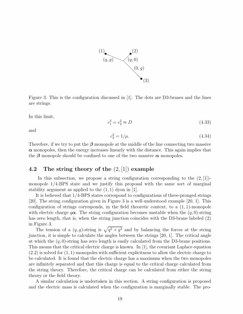
In this subsection, we propose a string configuration corresponding to the (2, [1])-monopole 1/4-BPS state and we justify this proposal with the same sort of marginalstability argument as applied to the (1, 1) dyon in [1].

It is believed that 1/4-BPS states correspond to configurations of three-pronged strings[20]. The string configuration given in Figure 3 is a well-understood example [20, 1]. Thisconfiguration of strings corresponds, in the field theoretic context, to a (1, 1)-monopolewith electric charge qα. The string configuration becomes unstable when the (q, 0)-stringhas zero length, that is, when the string junction coincides with the D3-brane labeled (2)in Figure 3.

The tension of a (q, g)-string is√

q2 + g2 and by balancing the forces at the stringjunction, it is simple to calculate the angles between the strings [20, 1]. The critical angleat which the (q, 0)-string has zero length is easily calculated from the D3-brane positions.This means that the critical electric charge is known. In [1], the covariant Laplace equation(2.2) is solved for (1, 1)-monopoles with sufficient explicitness to allow the electric charge tobe calculated. It is found that the electric charge has a maximum when the two monopolesare infinitely separated and that this charge is equal to the critical charge calculated fromthe string theory. Therefore, the critical charge can be calculated from either the stringtheory or the field theory.

A similar calculation is undertaken in this section. A string configuration is proposedand the electric mass is calculated when the configuration is marginally stable. The pro-

19

��

��

@@

@@t t

t

(1)

(2)

(3)

(0, 2g)

(q, g)(q, g)

(a)

��

��

@@

@@t t

t

-�

?

6

ν

µ

θ

(b)

Figure 4: These two pictures are of the Y-shaped string configuration, dots denote D3-branes and lines denote strings. (a) shows which string is which and (b) shows the lengthsµ and ν and the angle θ.

posed string configuration is Y-shaped and is shown in Figure 4. The angle θ can becalculated by balancing forces at the junction and is given by

sin θ =g

√

q2 + g2. (4.35)

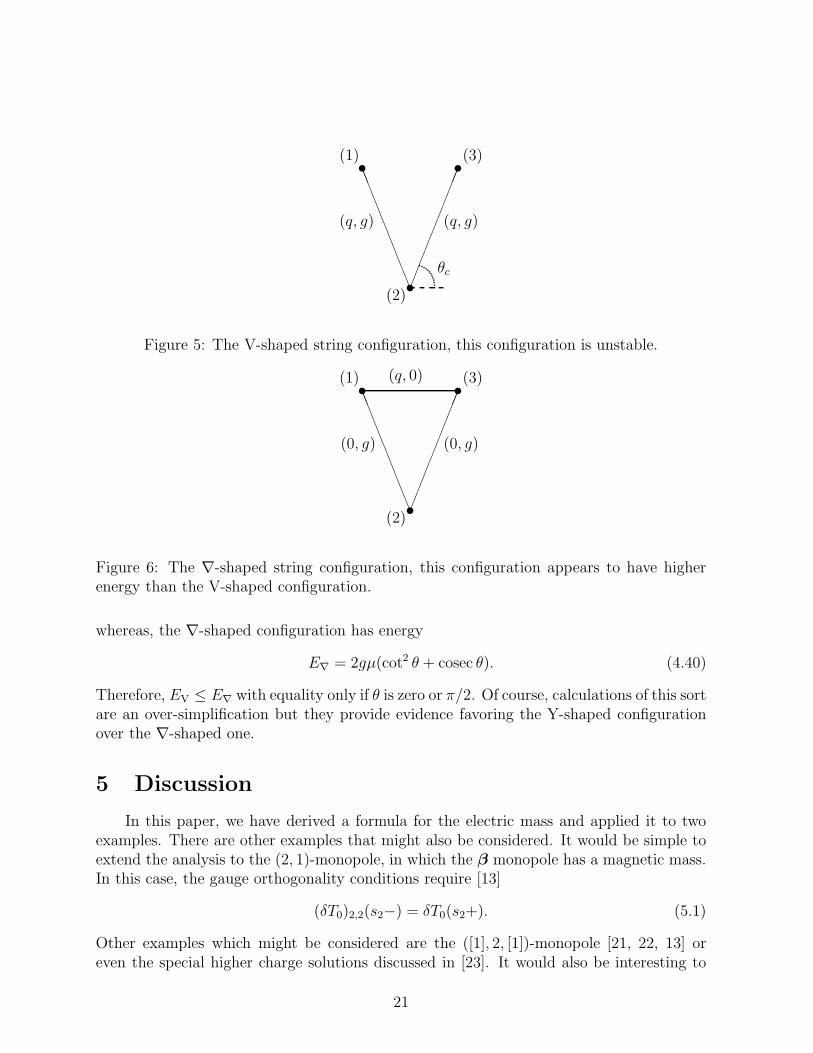
This configuration becomes unstable if the (0, 2g)-string has zero length and the Y-shapedegenerates to the V-shaped configuration illustrated in Figure 5. At the onset of instability

θ = θc (4.36)

wheresin θc =

µ√

(

1

2ν)2

+ µ2

. (4.37)

This means that the critical electric charge is qc where

qc =gν

2µ. (4.38)

From the string picture it would appear that this critical value of the electric charge is aminimum. This contrasts with the (1, 1) case, where the critical value is a maximum. Theabove value of the critical charge is identical to the charge obtained from (4.20) and (4.24).This critical value corresponds to the 1/4-BPS electric charge of infinitely separated twomassive monopoles, with the massless monopole on top of either massive monopole.

Figure 5 might create the suspicion that at some point the Y -shaped configuration haslarger energy than the ∇-shaped configuration illustrated in Figure 6. Calculating theenergies allays this concern. The V-shaped configuration has energy

EV = 2gµcosec2 θ = 2gµ(cot2 θ + 1) (4.39)

20

����������

LL

LL

LL

LL

LL

(1)

(2)

(3)

(q, g)(q, g)

θc

t t

t

Figure 5: The V-shaped string configuration, this configuration is unstable.

����������

LL

LL

LL

LL

LLt t

t

(1)

(2)

(3)

(0, g)(0, g)

(q, 0)

Figure 6: The ∇-shaped string configuration, this configuration appears to have higherenergy than the V-shaped configuration.

whereas, the ∇-shaped configuration has energy

E∇ = 2gµ(cot2 θ + cosec θ). (4.40)

Therefore, EV ≤ E∇ with equality only if θ is zero or π/2. Of course, calculations of this sortare an over-simplification but they provide evidence favoring the Y-shaped configurationover the ∇-shaped one.

5 Discussion

In this paper, we have derived a formula for the electric mass and applied it to twoexamples. There are other examples that might also be considered. It would be simple toextend the analysis to the (2, 1)-monopole, in which the β monopole has a magnetic mass.In this case, the gauge orthogonality conditions require [13]

(δT0)2,2(s2−) = δT0(s2+). (5.1)

Other examples which might be considered are the ([1], 2, [1])-monopole [21, 22, 13] oreven the special higher charge solutions discussed in [23]. It would also be interesting to

21

use the numerical ADHMN construction of [24] to find the a field. This would reveal thespatial distribution of the electric mass. This might be interesting in examples, like theone considered in this paper, where there are monopoles with no magnetic mass. It wouldalso be instructive in examples, such as those in [23], where there are extra minima of theHiggs field.

The dynamics of 1/4-BPS states are not fully understood. In the better understood(1, 1) example the level set of the potential lies on a group orbit. In the (2, [1]) example,this is not the case as there are monopoles with the same electric mass which cannot begroup transformed into each other. The geodesic motion on the Y space was studied byDancer and Leese [18]. It would be interesting to determine how this motion is modifiedby the presence of the potential.

Acknowledgment

CJH warmly thanks the Physics Department and Center for Theoretical Physics, SeoulNational University for hospitality while part of this work was undertaken. CJH thanksFitzwilliam College, Cambridge for a research fellowship and thanks Patrick Irwin and PaulSutcliffe for useful discussion. KL appreciates the Aspen Center for Physics, ColumbiaUniversity and PIMS of University of British Columbia for support and hospitality. KLis supported in part by the SRC program of SNU-CTP, the Basic Science and ResearchProgram under BRSI-98-2418, and KOSEF 1998 Interdisciplinary Research Grant 98-07-02-07-01-5.

References

[1] K. Lee and P. Yi, Phys. Rev. D 58 (1998) 066005, hep-th/9804174.

[2] D. Bak, K. Hashimoto, B.-H. Lee, H. Min and N. Sasakura, Phys. Rev. D 60 (1999)046005, hep-th/9901107; K. Hashimoto, H. Hata and N. Sasakura, Phys. Lett. B431 (1998) 303, hep-th/9803127; Nucl.Phys. B535 ((1998) 83, hep-th/9804164; T.Kawano and K. Okuyama, Phys. Lett. B 432 (1998) 338, hep-th/9804139.

[3] T. Ioannidou and P.M. Sutcliffe, Phys. Lett. B 467 (1999) 54. hep-th/9907157.

[4] D. Tong, Phys. Lett. B 460 (1999) 295, hep-th/9902005.

[5] A.S. Dancer, Commun. Math. Phys. 158 (1993) 545.

[6] A.S. Dancer, Nonlinearity 5 (1992) 1355.

[7] K. Lee, E.J. Weinberg, P. Yi, Phys. Rev. D 54 (1996) 6351, hep-th/9605229.

[8] K. Lee, Phys. Lett. B 458 (1999) 53, hep-th/9903095.

22

[9] D. Bak, C. Lee, K. Lee and P. Yi, Phys. Rev. D 61 (2000) 025001, hep-th/9906119.

[10] E.J. Weinberg, Nucl. Phys. B167 (1980) 500; Nucl. Phys. B 203 (1982) 445.

[11] W. Nahm, The construction of all self-dual multimonopoles by the ADHM method inMonopoles in quantum field theory edited by N.S. Craigie, P. Goddard and W. Nahm(World Scientific, Singapore, 1982).

[12] N.J. Hitchin, Commun. Math. Phys. 89 (1983) 145.

[13] C.J. Houghton, P. Irwin and A.J. Mountain, JHEP 9904 (1999) 029, hep-th/9902111.

[14] T.C. Kraan and P. van Baal, Phys. Lett. B 428 (1998) 268, hep-th/9802049.

[15] H. Osborn, Ann. Phys. (N.Y.) 135 (1981) 373.

[16] H. Nakajima, Monopoles and Nahm’s equations in Einstein metrics and Yang-Mills

connections edited by T. Mabuchi and S. Mukai (Marcel Dekker, New York, 1993).

[17] P. Irwin, Phys. Rev. D 56 (1997) 5200, hep-th/9704153.

[18] A.S. Dancer and R.A. Leese, Proc. R. Soc. Lond. A 440 (1993) 421.

[19] A.S. Dancer and R.A. Leese, Phys. Lett. 390B (1997) 252.

[20] O. Bergman, Nucl. Phys. B525 (1998) 104, hep-th/9712211.

[21] C.J. Houghton, Phys. Rev. D 56 (1997) 1220, hep-th/9702161.

[22] K. Lee and C. Lu, Phys. Rev. D 57 (1998) 5260, hep-th/9709080.

[23] C.J. Houghton and P.M. Sutcliffe, J. Maths. Phys. 38 (1997) 5576, hep-th/9708006.

[24] C.J. Houghton and P.M. Sutcliffe, Commun. Math. Phys. 180 (1996) 343,hep-th/9601146.

23