
Hot Wires Wakes and Drag Measurement
30
AAE 520 Experimental Aerodynamics Professor Schneider Experiment 1: Hot Wires, Wakes, and Drag Measurement Purdue University School of Aeronautics and Astronautics Performed by: Micah Chibana and Edward Kay 2/9/2004
Transcript of Hot Wires Wakes and Drag Measurement

AAE 520
Experimental Aerodynamics
Professor Schneider
Experiment 1:
Hot Wires, Wakes, and Drag Measurement
Purdue University
School of Aeronautics and Astronautics
Performed by: Micah Chibana and Edward Kay
2/9/2004

2
Hot Wires, Wakes, and Drag Measurement
1. Abstract
Using a subsonic wind tunnel, the wake of a cylinder and a NACA 0010 airfoil were
investigated using hot wire measurements of the air velocity downstream from the objects.
Integrating the profile of the velocity across the wake perpendicular to the flow gives a
measurement of the drag on the bodies. This technique was used to evaluate drag at
various velocities and at various positions downstream from the objects. The airfoil was
also studied at an angle of attack. In the performance of this lab we were able to gain
experience using hot wires and the related experimental equipment, while at the same
time obtaining experimental measurements of the drag coefficient, Cd, that were in
agreement with theoretical values. Other measurements confirmed that the cylinder wake
remains self-similar as it travels downstream.
2. Introduction
Whenever an object is moving in a fluid (or whenever a fluid is moving relative to an
object) at a large enough speed (Re > 1), there is always a wake trailing behind. This is
easily seen in the trailing wake behind boats as they drive through water. Often the fluid
flowing in this wake is turbulent and hard to predict without the use of experimental
techniques. Studying the velocities of the fluid in this wake can give a measurement of
the drag on the object. For most applications such as airplanes, boats, and cars the design
of the object’s shape is critical in reducing the drag on the object, thus creating a better
performing vehicle. Fluid mechanics gives a formulation of the physics behind fluid flow
and has largely studied the flow around cylinders. This forms the motivation behind our
study of cylinder wakes, due to the ease of comparison to theoretical predictions.
Measuring the wake of an airfoil should give a nice comparison/contrast to the cylinder,
giving a real world application to this experiment.1

3
2.1 Objectives
The objectives of the experiment were to:
o Observe the structure of a wake.
o Use velocity profile information to calculate the drag on a body.
o Become familiar with using a hot-wire anemometer.
o Compare the results from various cylinder and airfoil wakes, under
downstream conditions.
3. Background
3.1 Pitot-Static Tube
When studying the flow for an inviscid, incompressible fluid of density ρ along a
streamline, Bernoulli’s equation gives a relation between the static pressure (Ps), total
pressure (Pt), and the average velocity of the flow (U).2
Ps + ½ρU2 = Pt (1)
A pitot-static tube uses a pitot tube for measuring the total pressure and a static tube to
obtain a measurement of the static pressure (Fig.1). Once these two quantities are
measured equation 1 can be rewritten to obtain the value for the velocity of the fluid.1
(2)

4
Figure 1: A pitot–static tube is aligned along a streamline to give a measurement
of ∆P.1
3.2 Hot Wire Sensor
Another tool used in the measurement of fluid velocity is the hot wire sensor (Fig. 2). A
hot wire consists of a thin thread of wire placed perpendicular to the flow that is heated
and kept at a constant temperature by an anemometer. When the wire is placed in the
flow, the passing fluid cools the wire. Since the anemometer is keeping the wire at a
constant temperature, the voltage passing through the wire must increase when fluid is
passing. Thus, the anemometer measures the amount of heat transferred to the fluid from
the wire.
Figure 2: Hot wire sensor1
King’s Law gives an empirical formula relating the voltage applied to the wire (V) and
the velocity of the fluid (U).
(3)
3.3 Cylinder Wake: Laminar and Turbulent Flow
Flow around a cylinder has been a thoroughly studied topic in fluid mechanics. Figure 3
shows a variety of flow patterns as the velocity of the fluid is increased. The Reynolds
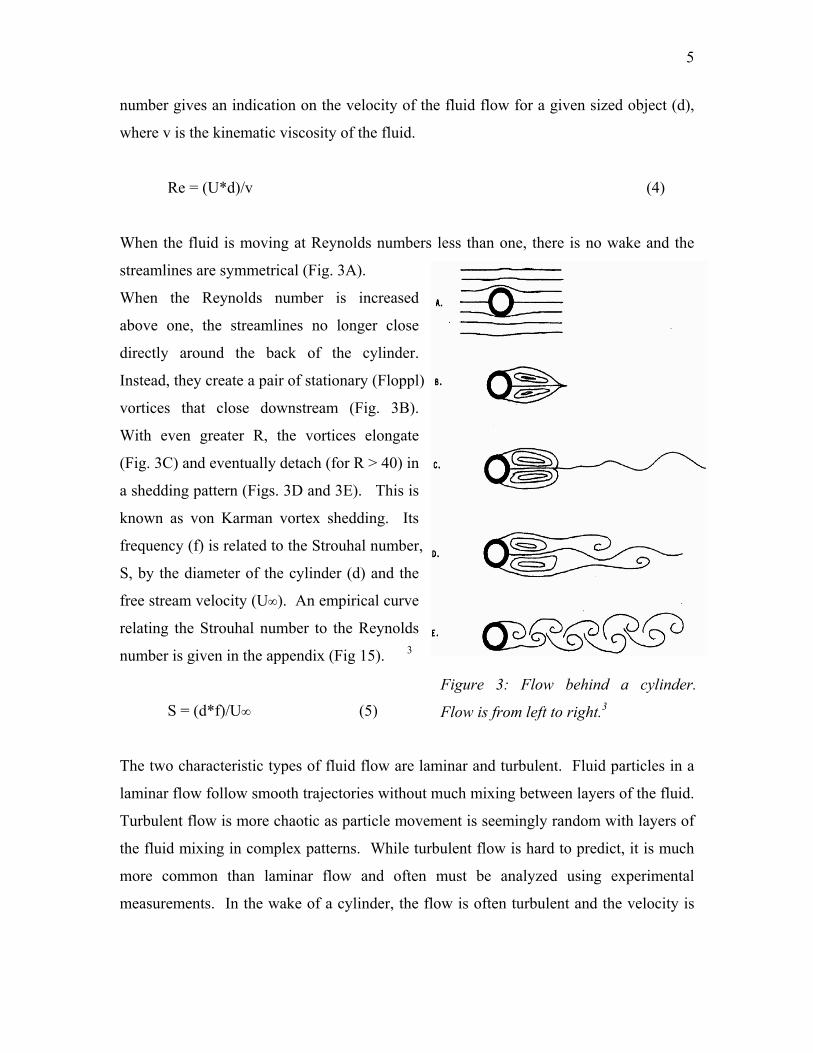
5
number gives an indication on the velocity of the fluid flow for a given sized object (d),
where v is the kinematic viscosity of the fluid.
Re = (U*d)/v (4)
When the fluid is moving at Reynolds numbers less than one, there is no wake and the
streamlines are symmetrical (Fig. 3A).
When the Reynolds number is increased
The two characteristic types luid
above one, the streamlines no longer close
directly around the back of the cylinder.
Instead, they create a pair of stationary (Floppl)
vortices that close downstream (Fig. 3B).
With even greater R, the vortices elongate
(Fig. 3C) and eventually detach (for R > 40) in
a shedding pattern (Figs. 3D and 3E). This is
known as von Karman vortex shedding. Its
frequency (f) is related to the Strouhal number,
S, by the diameter of the cylinder (d) and the
free stream velocity (U∞). An empirical curve
relating the Strouhal number to the Reynolds
number is given in the appendix (Fig 15). 3
S = (d*f)/U∞ (5)
Figure 3: Flow behind a cylinder.
Flow is from left to right.3
of f flow are laminar and turbulent. Fluid particles in a
laminar flow follow smooth trajectories without much mixing between layers of the fluid.
Turbulent flow is more chaotic as particle movement is seemingly random with layers of
the fluid mixing in complex patterns. While turbulent flow is hard to predict, it is much
more common than laminar flow and often must be analyzed using experimental
measurements. In the wake of a cylinder, the flow is often turbulent and the velocity is

6
lower than in the free stream. Figure 4 shows the turbulent wake behind a cylinder and
the profile of the velocity deficit in the wake.
Figure 4: Turbulent wake and velocity profile behind a cylinder3
This deficit can be viewed as energy lost from the free stream and integrating it across the
wake can give a measure of the total drag force acting on a body. Given the velocity
profile components (Fig. 5), the velocity deficit (u1) can be written as:
u1 = U∞ – u (6)
Figure 5: Geometry of the velocity profile in a wake3

7
Moving away from the wake u converges to U∞. The total drag (D) is found by
considering the conservation of momentum in a control volume enclosing the cylinder.
(7)
(8)
Here Eqn. 6 has been used to put Eqn. 7 in terms of the height of the body (h), velocity
deficit at point y (u1), and the fluid density (ρ). Another to express the drag force (D) is
in terms of the frontal area of the body (A) and the drag coefficient (Cd).
D = ½ρAU∞2Cd (9)
An empirical curve fit for the Cd of a cylinder is:
(10)
Another result from fluid mechanics is that as the velocity is observed downstream from
the cylinder the profile should remain self-similar in shape.
(11)
Thus, the curve shape should be independent of the downstream location given
x/(Cd*d) > 50. This self-similarity of the profile and the empirical curve for Cd will be
compared to results found in this lab.3

8
4. Procedure
4.1 Tunnel Setup
The diagram of the experimental setup is shown in figure 6, consisting of the subsonic
wind tunnel, pitot tube, manometer, hot wire, transversing mechanism, anemometer,
oscilloscope, and Fluke 77. The pitot tube is connected to the manometer for pressure
measurements as described in section 3.1. Downstream in the flow from the object being
studied is the hot wire which sits on a transversing mechanism. This allows the location
of the hot wire to be adjusted perpendicular to the free stream flow. A micrometer on the
mechanism allows for accurate position measurements. The anemometer keeps the hot
wire at a constant temperature while its output shows the voltage applied to the hot wire
on the oscilloscope display. The Fluke is also there for voltage measurements.
Figure 6: Wind tunnel and associated experimental setup.3

9
4.2 Anemometer Calibration
The first step before running any measurements with the hot wire is to do a calibration
run. The internal resistance of the anemometer is set at 1.25 times the resistance of the
hot wire probe’s cold resistance which is measured with the Fluke 77. Before the tunnel
is turned on, the manometer measurement of static pressure is noted. Manometer
readings for Pt are taken for various tunnel velocities and the corresponding anemometer
voltages are taken. This data will be used to fit a calibration curve, which will be used to
determine all velocities measured hereon.
4.3 Velocity Profile Measurements
For all the steps in this experiment, the following steps were taken to measure the
velocity profile downstream from an object. While running the tunnel at a given velocity,
either the cylinder or airfoil is placed upstream from the hot wire. Starting the wire near
the edge of the tunnel gives an indication of the free stream velocity. The hot wire is then
moved towards the center of the tunnel until the velocity changes. Note that the
anemometer voltage output is what is monitored as a function of the fluid velocity. Once
the edge of the wake is found, back the hot wire up slightly so that data will start in the
free stream. Measure the anemometer voltage and voltage rms on the oscilloscope noting
the location of the hot wire probe by reading the micrometer on the transversing
mechanism. The hot wire is moved at intervals across the wake noting the anemometer
voltage and probe location at each point. When the wire passes all the way through the
wake, the anemometer voltage will again reach the free stream value. This data can
readily be converted in velocity profile information.
This procedure of velocity profile measurement was followed for the following cases (all
TS numbers are in inches and refer to the diagram of the tunnel in the appendix figure 16):
10
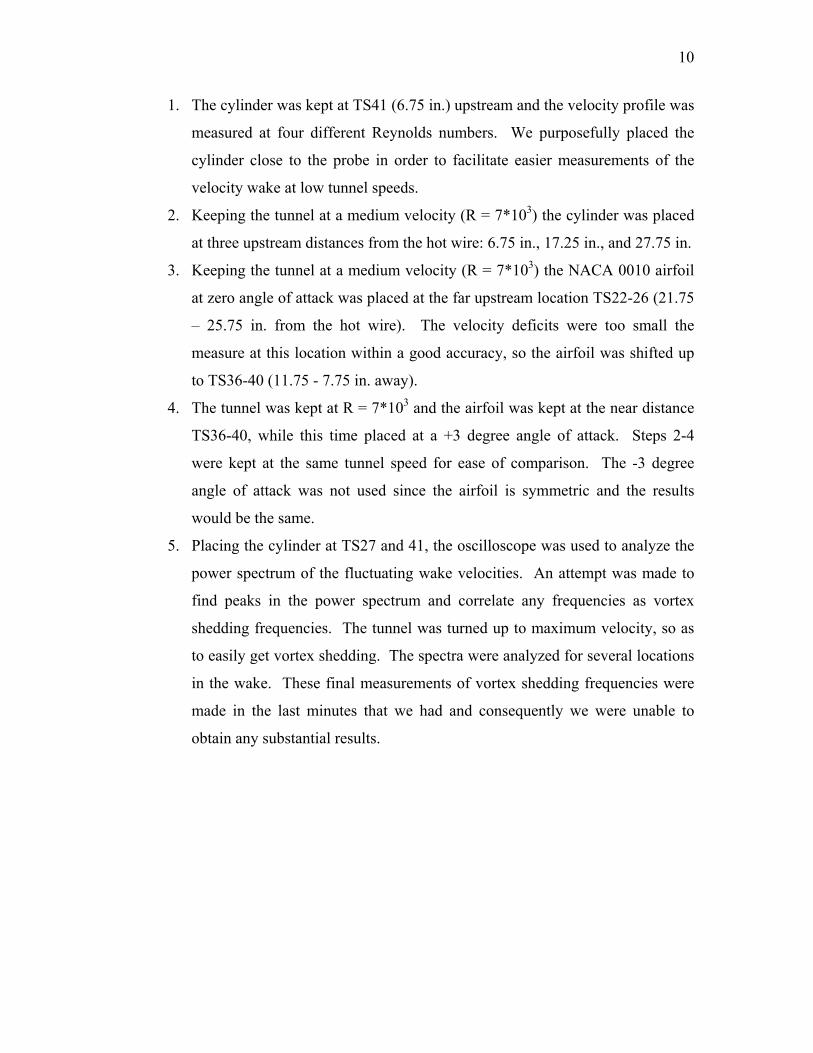
1. The cylinder was kept at TS41 (6.75 in.) upstream and the velocity profile was
measured at four different Reynolds numbers. We purposefully placed the
cylinder close to the probe in order to facilitate easier measurements of the
velocity wake at low tunnel speeds.
2. Keeping the tunnel at a medium velocity (R = 7*103) the cylinder was placed
at three upstream distances from the hot wire: 6.75 in., 17.25 in., and 27.75 in.
3. Keeping the tunnel at a medium velocity (R = 7*103) the NACA 0010 airfoil
at zero angle of attack was placed at the far upstream location TS22-26 (21.75
– 25.75 in. from the hot wire). The velocity deficits were too small the
measure at this location within a good accuracy, so the airfoil was shifted up
to TS36-40 (11.75 - 7.75 in. away).
4. The tunnel was kept at R = 7*103 and the airfoil was kept at the near distance
TS36-40, while this time placed at a +3 degree angle of attack. Steps 2-4
were kept at the same tunnel speed for ease of comparison. The -3 degree
angle of attack was not used since the airfoil is symmetric and the results
would be the same.
5. Placing the cylinder at TS27 and 41, the oscilloscope was used to analyze the
power spectrum of the fluctuating wake velocities. An attempt was made to
find peaks in the power spectrum and correlate any frequencies as vortex
shedding frequencies. The tunnel was turned up to maximum velocity, so as
to easily get vortex shedding. The spectra were analyzed for several locations
in the wake. These final measurements of vortex shedding frequencies were
made in the last minutes that we had and consequently we were unable to
obtain any substantial results.

11
5. Analysis of Results
5.1 Calibration
Fitting calibration data to King’s Law (Eqn. 3) and using a least squares fit line gave the
following calibration curves:
Day One Day Two
y=U^.5; x=V2 y = 0.6639x - 0.8055 y = 0.7192x - 0.8844
R2 0.9987 0.9973
Figure 7: Anemometer calibration results
Sample Calculation:
Ideal gas law: P = ρRT
Given ambient pressure (P), temperature (T), and the ideal gas constant (R=286); the density of air ρ =
P/RT = (99335 Pa)/(286 * 297.6 K) = 1.167 kg/m3
Manometer reading: Pt = 1.317 in. H2O * (249.09 Pa/1 in. H2O) = 328.1 Pa
Anemometer output voltage: 2.048 V
Using Eqn. 2 with Ps = 319.6 Pa:
U = [2*(328.1 Pa – 319.6 Pa)/ 1.1671 kg/m3]^.5 = 3.810 m/s
U is calculated from the various Pt measurements and then U^.5 is plotted versus V2 according to Eqn. 3.
Microsoft Excel was used to fit the least squares line, which solves the system of equations (m=A and
b=B):1
(12)
The R2 values indicate less than one percent error in the calibration of the anemometer.

12
5.2 Cylinder at TS41 for Various R
Figure 7 gives a picture of the velocity profiles for the cylinder at a distance of 6.75 in.
With increasing Reynolds numbers the height of the curve increases due to the increase in
the free stream velocity. Higher Reynolds numbers also show a steeper curve or velocity
deficit in the wake resulting in a larger value of drag. Conversion of raw anemometer
voltage data to fluid velocity was obtained through the use of the day one calibration
yielding a smooth picture of the profile. Another thing seen in Fig. 7 is that the center of
wake stay in the center of the tunnel (the wake stays symmetric).
Sample Calculation:
Anemometer voltage reading at location .1016 m = 2.52 V
Using day one calibration: U = [.6639*(2.52^2) - .8055]^2 = 11.7 m/s
Dynamic Viscosity (Sutherland’s Law): µ = mu0*[(T/T0)^(3/2)]*[(T0+198.6)/(T+198.6)]
µ = 3.74*10-7*[(535.67 Rankin/518.6 Rankin)^(3/2)]*[(518.6 R +198.6)/(535.67+198.6)] = 3.835 lb-s/ft^2
= 1.836*10-5 kg/m*s
Kinematic Viscosity: v = µ/ρ = (1.836 kg/m*s)/( 1.167 kg/m3) = 1.57*10-5 m2/s
Reynolds Number (Eqn. 4): R= U∞*d/v = (11.7 m/s * .0127 m)/(1.57*10-5 m2/s) = 9400
These U values correspond to u in Eqn. 7 and can be integrated using the trapezoidal
method giving the drag, D. Eqn. 9 can then be rearranged to find Cd. Figure 8 gives a
tabular result for the four Cd values found at TS41 and compares them to theoretically
obtained values found through Eqn. 10.

13
Velocity Wake Profiles of a Cylinder
34
56
789
1011
1213
0.09 0.11 0.13 0.15 0.17 0.19
Position (m)
Velo
city
(m/s
)
Re 9400 Re 7300 Re 6000 Re 4800
Figure 7: Velocity profiles for the cylinder at location TS41 (6.75 in. from the hot
wire).
Reynolds Number
Experimental Cd
Theoretical Cd
Percent Error
9400 1.041 +- .027 1.022 2% 7300 1.038 +- .022 1.027 1% 6000 1.034 +- .026 1.030 <1% 4800 0.939 +- .024 1.035 -9%
Figure 8: Cd results for the cylinder at TS41
Sample Calculation:
Experimental Cd: Trapezoidal method of integration used for Eqn. 7. f(y) = u*(U∞-u)
For R = 9400 at TS41, U∞ = 11.7 m/s. f(y) is computed at each location and then f(y) is integrated across
the wake (only this area needs to be integrated since u goes to U∞ outside of the wake). The trapezoidal
method of integration is:
(13)
For this sample calculation a =.1016 m, b =.1778, x is the position, and y is u*(U∞-u) calculated at location
x. The step size in x = xi+1 – xi = .00635 m.

14
The integral of f(y) = .5*(.00635)*[0 + 2(1.9 + 5.4 + 17.0 + 18.8 + 24.5 + 25.8 + 23.4 + 15.2 + 6.0 + 3.1
+ .5) + 0] = .9 = D/(h*ρ) from Eqn. 7.
In Eqn. 10, A = h*d. Rearranging gives
Cd = 2*[D/(h* ρ)]*[1/(d*U∞2)] = 2*(.9)*{1/[.0127m *(11.7m/s)2]} = 1.041
Theoretical Cd (Eqn. 10): Cd = 1 + 10.0*R^(-2/3) = 1 + 10.0*(9400)^-(2/3) = 1.022
Percentage Error = [(Experimental Cd – Theoretical Cd)/(Theoretical Cd)]*100 = [(1.041-
1.022)/(1.022)]*100 = 2%
The only result experimental Cd result in agreement with theory is for R = 6000,
although all are within 2% except for R = 4800. Perhaps we have underestimated the
precision of our Cd measurement. It is logical to have worse results at low velocities
because the velocity deficit is smaller and thus harder to measure. I might also note that
the R = 4800 measurement was the first one of the experiment, so there may be a
significant amount of experimental error associated with that measurement.
Contrastingly, at high velocities the amount of turbulence is higher in the wake
contributing to an imprecision in measuring the velocity. This is why our mid-range data
seems to fit best. The imprecision experimental Cd stems from computational error of
the trapezoidal rule, velocity fluctuations due to turbulence, and a level of ambiguity
associated with selecting U∞. The trapezoidal rule error is order (1/N2) for N number of
intervals. We have used this as a rough error estimate for the integration and have
propagated it through the experimental Cd calculation. It can be observed in the wake
profiles in Fig. 7 that the velocity measurements at the both sides of the wake are not
exactly equivalent, thus resulting in an error in selecting the free stream velocity.
Sample Calculation:
Error in U∞: ∆U∞ = U∞*[(4*∆V)/V] = 11.7 m/s *[(4*.005 V)/2.522 V] = .1 m/s
Error in trapezoidal rule: ∆ [D/(h*ρ)] ≈1/N2 = (1/112) = .008
∆(Cd) ≈ Cd*[2*( ∆U∞/U∞) + {∆ [D/(h*ρ)]/ [D/(h*ρ)]}] = 1.041*[(2*.1m/s)/11.7 m/s + (.008/.9)] = .027
5.3 Cylinder at Various Downstream Positions for R = 7000

15
Three velocity profiles were measures for positions at TS41, 30.5, and 20 (6.75 in., 17.25
in., and 27.75 in. from the hot wire). The velocities u in the wakes were computed using
the same method as above. Closer to the cylinder (TS41) the profile is thin and the
deficit is large (Fig.8). As the wake travels downstream it broadens while as the same
time keeping the same geometry and the same drag (related the integral of the velocity
deficit by Eqn. 8). This confirms the theoretical picture of a cylinder wake spreading
downstream presented in Fig. 4. Also from Fig.8 it is noted that since the curves are all
centered around the same location, the wake travels straight downstream.
Wake Profiles of a Cylinder at Various Downstream Locations
6
6.5
7
7.5
8
8.5
9
0.05 0.07 0.09 0.11 0.13 0.15 0.17 0.19 0.21 0.23
Position (m)
Vel
ocity
(m/s
)
TS41 TS30.5 TS20
Figure 8: Wake Profiles of a Cylinder at Various Downstream Locations for
R=7000
Eqn. 6 takes the velocities u and puts them in terms of the velocity deficit u1 and Eqn. 11
gives a relation for analyzing the self-similarity of the profiles by normalizing the width
and height of the profiles. Experimental results along with the theoretical curve are given
in Fig. 9.

16
Self-Similarity of Cylinder Wake for Various Downstream Positions
-0.1
0.1
0.3
0.5
0.7
0.9
1.1
-1.25 -0.75 -0.25 0.25 0.75 1.25
y/b
{u1(
y/b)
}/u1m
ax
TS 41 TS 30.5 TS 20 Theoretical: u1/u1max = [1-(y/b)^1.5}^2
Figure 9: Self-Similarity of Cylinder Wake for Various Downstream Positions at
R = 700
Sample Calculation:
At TS41: velocity u = 8.5 m/s at location y = .10668 m
(this is the second diamond point from the left in Fig. 9)
b = .03937 m, U∞ = 8.6 m/s, y0 (middle of the tunnel) = .13843 m
u1 = U∞ - u = 8.6 m/s – 8.5m/s = .1m/s (after all u1 calculated find u1max = 2.06152m)
u1/u1max = (.1m/s)/(2.06152m) = .07
y/b = (.10668 m - .13843m)/.03937 m = -.80645
The plot in Fig. 9 indicates that we were able to confirm the theoretical self-
similar relation given in Eqn. 11. The experimental values vary just slightly even as you
continue downstream. As in Sec. 5.2, the velocity profile can be used for measuring Cd.

17
Distance from Hot
Wire (in.)
Experimental
Cd
Theoretical
Cd Percent Error
6.75 1.041 +- .024 1.027 1%
17.25 1.038 +- .023 1.028 1%
27.75 1.129 +- .026 1.027 10%
Figure 10: Cd at Various Distances from the Cylinder at R = 7000
The closer measurements are in agreement with the theoretical values, but the farthest
measurement does not since the accuracy of measuring the velocity profile of the wake
goes down as you move away from the cylinder. As shown in Fig. 8 as the wake moves
downstream, the velocity profile broadens and the velocity deficit decreases. When
further downstream the hot wire must traverse a larger distance and the velocity values
are harder to measure causing the absolute error increases. This problem of measuring a
small velocity deficit was the same as encountered in measuring the wake a low Reynolds
numbers in Sec. 5.2.
5.4 Drag on a NACA 0010 Airfoil
As described in the procedure, the NACA 0010 airfoil wake was observed at the same
free stream velocity (8.4 m/s) as the cylinder though this results in a higher Reynolds
number (R = 55700) since the chord length is 4 in. and not the ½ in. diameter of the
cylinder. First the airfoil was placed farther away from the hot wire, but this resulted in
small variations of the velocity for the velocity deficit (as noted for the cylinder, if the
downstream distance is too far the data is off significantly). This velocity profile is
uneven and not useful, but can be observed in the appendix. Moving the airfoil closer to
the hot wire (7.75 in. from the trailing edge) produced very good results. Fig. 11 plots
the velocity profile of the airfoil at this location for both 0 and +3 degrees angle of attack.

18
Effect of Angle of Attack on the Wake Profile of the NACA 0010 Airfoil
7.4
7.6
7.8
8
8.2
8.4
8.6
8.8
0.11 0.12 0.13 0.14 0.15 0.16
Pos ition (m )
Vel
ocity
(m/s
)
Alpha = 0 Alpha = +3
Figure 11: Velocity Profile for the Airfoil Trailing Edge 7.75 in. from the Hot
Wire with the Airfoil at 0 and +3 degrees Angle of Attack.
Zero angle of attack results in a thinner wake with a higher u1max, while at +3 degrees
angle of attack the velocity profile is shifted over and broadened. Although the zero
angle of attack profile has a larger maximum deficit, the profile at an angle of attack
produces more drag as indicated in Fig. 12.
Angle of Attack (deg) Experimental CD
Theoretical CD
(found using Xfoil) Percent Error
0 0.0154 +- .0014 0.0166 +- .007 -7%
3 0.0178 +- .0007 0.0195 +- .007 -9%
Figure 12: Experimental and Theoretical Results for Airfoil at
R = 55700 and 7.75 in. to the Trailing Edge.
The experimental Cd result at zero angle of attack is in agreement with the theoretical
and the +3 degree result is quite close. The larger percent error is again due to the fact

19
that the velocity deficit being measured is quite small compared to the fluctuations. If we
were to repeat this lab, we would measure the airfoil drag at the maximum tunnel speed.
Comparing to the cylinder, the drag is reduced considerable. Also, the percentage error is
greater for the +3 degrees angle of attack because the wake is wider and the deficit
shallower than at 0 angle of attack. Looking through literature, we could not find a
comparable experiment at this Reynolds number, so we did a numerical simulation using
Xfoil. The error for the Xfoil is roughly taken from the Cl at zero angle of attack (-.0067),
which should be zero. Both Xfoil runs for the NACA 0010 at 0 and +3 degrees are
placed in the appendix.
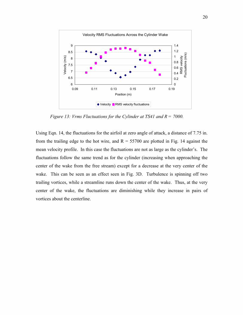
5.5 RMS Fluctuations
For all the velocity profile measurements, data was taken for the fluctuations (V’) in the
mean voltage (V). This gives a measure of how much the velocity is fluctuating and the
turbulence levels in the wake. Measuring these fluctuations across the wake presents a
picture of how turbulence is ordered in the wake. Assuming small fluctuations, voltage
fluctuations can be converted into velocity fluctuations (U’).3
(14)
Sample Calculations:
Cylinder at TS41 and R = 7000
At location y = .1016m, V = 2.302 V, V’ = .022 V, Calibration Day Two: A = .7192 and B = -.8844
Using Eqn. 14: U’ = 4[.7192(2.302)2 -.8844]*.7192*2.302*.022 = .43 m/s
The velocity fluctuations for the cylinder wake at TS41 and R = 7000 are plotted along
with the velocity profile in Fig. 13. The RMS fluctuation scale is on the right side, while
the left side has the mean velocity scale. The fluctuations increase as you go into the
wake and reach a maximum at the middle of the wake. The turbulence is in the middle of
the wake and dies out as you go farther from the center.
20
Velocity RMS Fluctuations Across the Cylinder Wake
6
6.5
7
7.5
8
8.5
9
0.09 0.11 0.13 0.15 0.17 0.19
Position (m)
Velo
city
(m/s
)
0
0.2
0.4
0.6
0.8
1
1.2
1.4
RM
S v
eloc
ity
Fluc
tuat
ions
(m/s
)
Velocity RMS velocity fluctuations
Figure 13: Vrms Fluctuations for the Cylinder at TS41 and R = 7000.
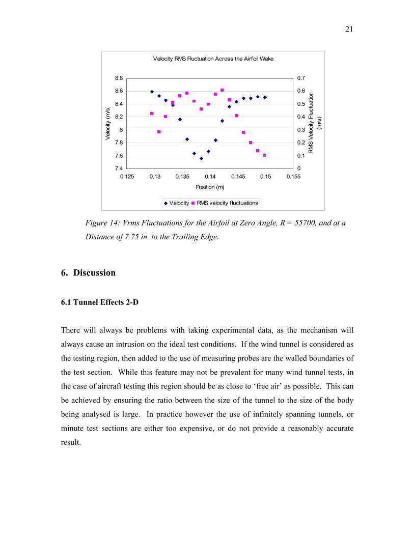
Using Eqn. 14, the fluctuations for the airfoil at zero angle of attack, a distance of 7.75 in.
from the trailing edge to the hot wire, and R = 55700 are plotted in Fig. 14 against the
mean velocity profile. In this case the fluctuations are not as large as the cylinder’s. The
fluctuations follow the same trend as for the cylinder (increasing when approaching the
center of the wake from the free stream) except for a decrease at the very center of the
wake. This can be seen as an effect seen in Fig. 3D. Turbulence is spinning off two
trailing vortices, while a streamline runs down the center of the wake. Thus, at the very
center of the wake, the fluctuations are diminishing while they increase in pairs of
vortices about the centerline.
21
Velocity RMS Fluctuation Across the Airfoil Wake
7.4
7.6
7.8
8
8.2
8.4
8.6
8.8
0.125 0.13 0.135 0.14 0.145 0.15 0.155
Position (m)
Velo
city
(m/s
)
0
0.1
0.2
0.3
0.4
0.5
0.6
0.7
RM
S Ve
loci
ty F
luct
uatio
n(m
/s)
Velocity RMS velocity fluctuations
Figure 14: Vrms Fluctuations for the Airfoil at Zero Angle, R = 55700, and at a
Distance of 7.75 in. to the Trailing Edge.
6. Discussion
6.1 Tunnel Effects 2-D
There will always be problems with taking experimental data, as the mechanism will
always cause an intrusion on the ideal test conditions. If the wind tunnel is considered as
the testing region, then added to the use of measuring probes are the walled boundaries of
the test section. While this feature may not be prevalent for many wind tunnel tests, in
the case of aircraft testing this region should be as close to ‘free air’ as possible. This can
be achieved by ensuring the ratio between the size of the tunnel to the size of the body
being analysed is large. In practice however the use of infinitely spanning tunnels, or
minute test sections are either too expensive, or do not provide a reasonably accurate
result.

22
One major feature of tunnel scale effect was that of the walls affecting the wake profile.
That is to say, not the boundary layer interaction, but the region of air that lies between
the ‘edge’ of the wake profile and the tunnel wall. While the relative size of the body
with respect to the tunnel dimensions was small, it must be noted that the wake extended
much further from the body that the diameter of cylinder, or the profile thickness of the
Airfoil. As the wake contains flow that has lower velocity than the surrounding flow,
according to Bernoulli’s principle for an Ideal fluid, the flow region around the wake
must accelerate to a higher velocity in order to satisfy the continuity equation. While air
is far from being an Ideal fluid, it is safe to assume that at such a low Reynolds number
the effects of compressibility will not have a great effect.
AIR
Figure 15a: (Left) Streamlines produced around a cylinder using a Potential
function (doublet+ freestream). Figure 15b. (Right) schematic of the velocity
distribution behind a cylinder in a test section
We can analyse the effect of a bluff body in a flow field by using potential flow, shown
in Figure 15a. The effect of combining a uniform flow field with a doublet causes
streamlines to separate from the central flow region. Coupled with the restriction of the
walls on either side must cause the flow to increase in velocity. The downstream effect
of this phenomenon is shown in figure 15b , where the solid line represents a standard
velocity profile taken from our results, and the dashed line represents the velocity profile
if there were no cylinder upstream. The question that therefore still remains is where to
take the value for the freestream velocity measurement in order to provide the baseline
for the drag integration.

23
During the investigation a lot of care was taken with the initial freestream measurement.
As this was the potential source of the greatest error in the drag calculation. The
freestream measurement was taken far out of the downstream wake of the cylinder
towards the wall where a reasonably accurate result could be obtained.
Excess
AIR
Figure 16: Location of freestream velocity measurement in order to gain more
accurate results.
It was hoped that by taking a measurement of the freestream at this location the excess
portion of the wake profile, shown in figure 16 would not be measured, which would give
a better estimate of the drag. However, since the freestream was measured while the
cylinder was in the tunnel, this would account for the general trend in our results giving
higher estimations of drag than previously measured empirical data, or CFD data. There
was still also a great deal of ambiguity of where to take this freestream value.
6.2 Vortex Shedding Frequencies
After a short investigation into the vortex shedding behaviour of the cylinder it was clear
from the oscilloscope readings that no frequencies that would reasonably be caused by a
set of shedding vortices could be found. Two locations were used in the investigation,
where the data from the TS27 location has been included in the appendix. Using both the
fast Fourier transform function provided by the Lecroy oscilloscope, and a further
24
averaged FFT from the captured data, only peaks at much higher frequencies could be
found. These plots have been included in the appendix, but no supportable conclusions
can be gained from them.
7. Conclusions
Anemometer calibrations followed theoretical expectations from King’s Law (Eqn. 3)
and were quite accurate with R2 values around .998 giving A and B with little to no error.
A majority of our Cd measurements for both the cylinder and airfoil were in agreement
with theoretical results given the precision of the experiment. Those results that were not
in agreement were cases where the velocity deficit was too small and difficult to measure.
These cases occurred at large downstream distances and low free stream velocity levels.
A majority of the Cd results were within 1 or 2% error, which is quite appreciable. Only
two cases had errors larger than this: the cylinder at R = 4800 and at 27.75 in. distance
downstream. Qualitatively, we observed the cylinder wake broaden while the velocity
deficit decreased as the downstream location was increased. The Eqn. 11 self-similarity
relation for wake profiles was confirmed for three locations downstream from the
cylinder. These results turned out particularly nicely.
The zero angle airfoil drag measurement was in agreements with our computational
measurement using Xfoil. The Cd result for +3 degrees was not in agreements, but was
very close. Percentage errors in airfoil drag were quite larger than cylinder (~8%
compared to 2%) and this was due to the difficulty in measuring the smaller velocity
deficits. The airfoil geometry is quite advantageous as it results in 1% of the drag created
by the cylinder. Fig. 11 shows that the effect of the angle of attack is to clearly shift the
wake, broaden it, which results in a larger Cd. Since the tunnel and airfoil are
symmetrical, we did not perform the experiment at -3 degrees since it should give the
same result.
25
Another indication of what is going on in the wake is Figs. 13 and 14, which show the
velocity fluctuations while crossing the wake. The cylinder had turbulence levels high at
the center the wake and trailing off when approaching the outer edges. The airfoil
fluctuations follow the same pattern, but with a dip in the center of the wake associated
with a calm streamline down the center as seen in Fig. 3D.
The majority of error in this lab is due to fact that the velocity levels are turbulent and
fluctuating. This creates and inherent precision error in all velocity measurements. Other
lower factor errors are due to error when performing the trapezoid method of integration.
This could be reduced by taking more intervals or using a different, more accurate
method of integration. Another error is due to a level of ambiguity when deciding the
free stream velocity. In many runs the free stream is smaller on far side of the tunnel.
This could be due to the fact that the hot wire is traversing across the wake and
interacting with the wake velocities. To correct for this, maybe we should have taken a
run across the tunnel at several velocities without any object in the tunnel. This would
give an indication to the level of uniformity in the free stream velocity and correct for
interactions between our measure instrument (the hot wire and traversing mechanism)
and the fluid flow. All in all, this lab made it quite easy to visualize what occurs in a
wake behind an object and allowed for fairly accurate measurements of Cd, which were
mostly within 2% of theoretical values.
8. References
1. “Background Information for Use of Pitot Tube, Manometer, Hot Wires, and
Hot Films.” AAE520. Purdue University. 2004.
2. Currie, I.G. Fundamental Mechanics of Fluids, 3rd ed, Marcel Dekker, Inc.,
New 2003York,.
3. “Hot Wires, Wakes, and Drag Measurement.” AAE520. Purdue University.
2004.

26
4. Xfoil 6.94 executable for Win32, optimized for Pentium 4.
http://raphael.mit.edu/xfoil/
9. Appendix
Figure 17: Empirical Correlation between Strouhal Number and Reynolds
Number.

27
Figure 18: Diagram of Wake Tunnel and Various Test Section Positions
Day One: Anemometer Callibration
y = 0.6639x - 0.8055R2 = 0.9987
1.75
1.95
2.15
2.35
2.55
2.75
2.95
3.15
3.35
4 4.5 5 5.5 6 6.5
Voltage^2 (V^2)
Velo
city
^.5
(m/s
)^.5
Volts^2 Linear (Volts^2)
Figure 19: Anemometer Calibration for Day One

28
Day Two:Anemometer Callibration y = 0.7192x - 0.8844
R2 = 0.9973
1.5
2
2.5
3
3.5
4
3.5 4.0 4.5 5.0 5.5 6.0 6.5
Voltage^2 (V^2)
Velo
city
^.5
(m/s
)^.5
volts^2 Linear (volts^2)
Figure 20: Anemometer Calibration for Day Two
Airfoil at TS22-26:Medium Velocity
7.8
7.9
8
8.1
8.2
8.3
8.4
8.5
8.6
0.11 0.115 0.12 0.125 0.13 0.135 0.14 0.145 0.15 0.155 0.16
Position (m)
Velo
city
(m/s
)
Figure 21: Airfoil at R = 55700, Zero Angle, and at Far Location

29
Figure 22: Xfoil Run Simulation of NACA 0010 at Zero Angle of Attack.

30
Figure 23: Xfoil Run Simulation of NACA 0010 at +3 Degrees Angle of Attack.
Figure 24a: Average FFT for location TS27 using MATLAB. Figure 24b: An
FFT plot and an Average FFT plot using the Lecroy oscilloscope at location TS27