Hornsea Project Three Offshore Wind Farm · mapping or assessing woodland structure and composition...
68
Hornsea Project Three Offshore Wind Farm Hornsea Project Three Offshore Wind Farm Appendix 6 to Deadline 2 Submission – Estimating Seabird Flight Height Using LiDAR (Cook et al, 2018) Date: 21 st November 2018
Transcript of Hornsea Project Three Offshore Wind Farm · mapping or assessing woodland structure and composition...
Hornsea Project Three Offshore Wind Farm
Hornsea Project Three
Offshore Wind Farm
Appendix 6 to Deadline 2 Submission –
Estimating Seabird Flight Height Using LiDAR (Cook et al, 2018)
Date: 21st November 2018
Estimating Seabird Flight Height Using LiDAR November 2018
i
Document Control
Document Properties
Organisation Ørsted Hornsea Project Three
Author Cook et al, 2018
Checked by n/a
Approved by n/a
Title Appendix 6 to Deadline 2 Submission –
Estimating Seabird Flight Height Using LiDAR (Cook et al, 2018)
PINS Document Number
n/a
Version History
Date Version Status Description / Changes
21/11/2018 A Final Submitted at Deadline 2 (21/11/2018)
Ørsted
5 Howick Place,
London, SW1P 1WG
© Ørsted Power (UK) Ltd, 2018. All rights reserved
Front cover picture: Kite surfer near a UK offshore wind farm © Ørsted Hornsea Project Three (UK) Ltd., 2018.
Estimating Seabird Flight Height using
LiDAR
Scottish Marine and Freshwater Science Vol 9 No 14
A S C P Cook, R M Ward, W S Hansen and L Larsen
Estimating Seabird Flight Height Using LiDAR
Scottish Marine and Freshwater Science Vol 9 No 14
Aonghais S C P Cook, Robin M Ward, William S Hansen and
Laurids Larsen
Report of work carried out by the British Trust for Ornithology and NIRAS Consulting
Ltd, on behalf of the Scottish Government
August 2018
Published by Marine Scotland Science
ISSN: 2043-7722
DOI: 10.7489/12131-1

Marine Scotland is the directorate of the Scottish Government responsible for the
integrated management of Scotland’s seas. Marine Scotland Science (formerly
Fisheries Research Services) provides expert scientific and technical advice on
marine and fisheries issues. Scottish Marine and Freshwater Science is a series of
reports that publishes results of research and monitoring carried out by Marine
Scotland Science. It also publishes the results of marine and freshwater scientific
work that has been carried out for Marine Scotland under external commission.
These reports are not subject to formal external peer-review.
This report presents the results of marine and freshwater scientific work carried out
for Marine Scotland under external commission.
© Crown copyright 2018
You may re-use this information (excluding logos and images) free of charge in any
format or medium, under the terms of the Open Government Licence. To view this
licence, visit: http://www.nationalarchives.gov.uk/doc/open-
governmentlicence/version/3/ or email: psi@nationalarchives,gsi.gov.uk
Where we have identified any third party copyright information you will need to obtain
permission from the copyright holders concerned.
Estimating Seabird Flight Height Using LiDAR
Aonghais S C P Cook, Robin M Ward, William S Hansen and
Laurids R Larsen
British Trust for Ornithology and NIRAS Consulting Ltd
Executive Summary
Accurately estimating the proportion of birds at collision risk height forms a key part
of assessing potential collision risk at offshore wind farms. Recent advances in
LiDAR and digital aerial imaging offer the potential to collect precise estimates of the
altitude of birds in flight. We trialled LiDAR and digital aerial photography as an
approach to measuring the flight heights of seabirds in the Outer Forth and Tay
Estuaries and carried out an exercise to validate measurements of flight height
gained from LiDAR. The validation exercise demonstrated that the height of birds in
flight could be measured using LiDAR to an accuracy of within 1 m. This compares
very favourably to other approaches used for measure seabird flight height.
We successfully collected flight height information on 2,201 birds of which 806 were
believed to be black-legged kittiwakes and 377 were identified as northern gannets.
These data were used to derive continuous flight height distributions. We also
demonstrate how data can be used to plot spatial patterns in seabird flight heights
which may be of use for the purposes of marine spatial planning. Based on our
experiences, we provide recommendations for the best practice in the use of LiDAR
to collect seabird flight height data as part of future studies.
Contents
Introduction ............................................................................................................................................ 1
Background ............................................................................................................. 1
How LiDAR works ................................................................................................... 1
Types of LiDAR System .......................................................................................... 2
Ecological Applications of LiDAR ............................................................................ 3
Project Objectives and Aims ................................................................................... 4
Methods ................................................................................................................................................. 6
Survey Area ............................................................................................................ 6
Survey ..................................................................................................................... 7
Equipment ............................................................................................................... 8
Validation Exercise ................................................................................................. 8
Data Processing ...................................................................................................... 9
Simulations ........................................................................................................... 10
Flight Height Modelling ......................................................................................... 11
Comparison with Previous Studies ....................................................................... 12
Three-dimensional modelling of black-legged kittiwake and gull flight heights ..... 13
Results ................................................................................................................................................. 14
Data Collection ...................................................................................................... 14
Data validation ...................................................................................................... 19
Simulations ........................................................................................................... 21
Visual comparison of simulated data and distributions fitted to these data ...................... 22
Comparison of predicted and observed proportions of birds from simulated datasets
within collision risk window ....................................................................................................... 23
Difference between simulated datasets and fitted distributions .......................................... 25
Flight Height Modelling ......................................................................................... 26
Proportions of birds at Collision Risk Height ......................................................... 31
Comparison with boat-based and digital aerial survey data .................................. 32
Comparison with the results of Cleasby et al. (2015) for northern gannet ............ 34
Three dimensional modelling of black-legged kittiwake flight height ..................... 36
Three dimensional modelling of gull flight height .................................................. 36
Discussion ........................................................................................................................................... 38
Future applications ................................................................................................ 41
Best practice recommendations ............................................................................ 43

Acknowledgements ............................................................................................................................ 46
References .......................................................................................................................................... 47
APPENDIX 1: Validation exercise ................................................................................................... 52
1
Introduction
Background
Scotland is recognised as having considerable potential for offshore renewable
energy development and the Scottish Government has the duty to ensure that the
development of offshore renewable sectors is achieved in a sustainable manner.
Strategic Environmental Assessments (SEAs) and Environmental Impact
Assessments (EIAs) for offshore renewable developments have identified a need to
evaluate potential interactions between offshore renewables and marine wildlife as a
matter of priority so that appropriate mitigation can be investigated and applied.
Collision mortality is widely regarded to be one of the main potential impacts of wind
farms on seabird populations (Furness et al., 2013; Garthe and Huppop, 2004).
Consequently concerns with respect to the potential collision impacts of offshore
wind farms have formed a substantial component of the consenting process for
offshore wind farm projects throughout the UK.
Estimates of collision risk are calculated using collision risk modelling; typically using
the Band model (Band, 2012). A key input parameter into the Band model is the
height at which birds fly. A range of methods exist for either measuring or estimating
bird flight heights, but validation of these flight heights appears to be limited or
lacking (Thaxter et al., 2016), resulting in considerable uncertainty over the
estimation of collision rates, and this may result in overly precautionary assessment
methods being applied (Furness et al., 2013). For one of the Band model options
(‘Option 3’), the risk of collision, with respect to the sweep of the turbines blades, is
calculated to reflect the heterogeneous likelihood of being struck, i.e. to account for
birds’ expected flight height distributions (Johnston et al., 2014) (other options
assume a homogenous likelihood of collision across the turbine blades). There is a
clear and growing need for the validation of the estimates of flight heights, collection
of robust data and quantification of the uncertainty around the data and subsequent
estimates (Johnston et al., 2014; Johnston and Cook, 2016; Thaxter et al., 2016).
Recent developments in the application of Light Detection and Ranging (LiDAR)
technology offer the potential to collect precise species specific estimates of seabird
flight heights when combined with the use of digital imagery in order to identify
individual birds to species level.
How LiDAR Works
LiDAR is a remote sensing technique. LiDAR systems record the three-dimensional
location of objects by emitting frequent, short-duration laser pulses. Each pulse is
2
reflected off an object and the time it takes to return to the LiDAR sensor is recorded.
The distance between the LiDAR and the object can then be calculated by
multiplying the time it takes for the pulse to return to the sensor by the speed of light
and dividing by two, in order to account for the return journey (Lefsky et al., 2002).
Each emitted laser pulse is aimed towards a different location and, by aggregating
the large number of resulting pulse signal return records, a detailed three
dimensional map of surface structure can be created. When LiDAR equipment are
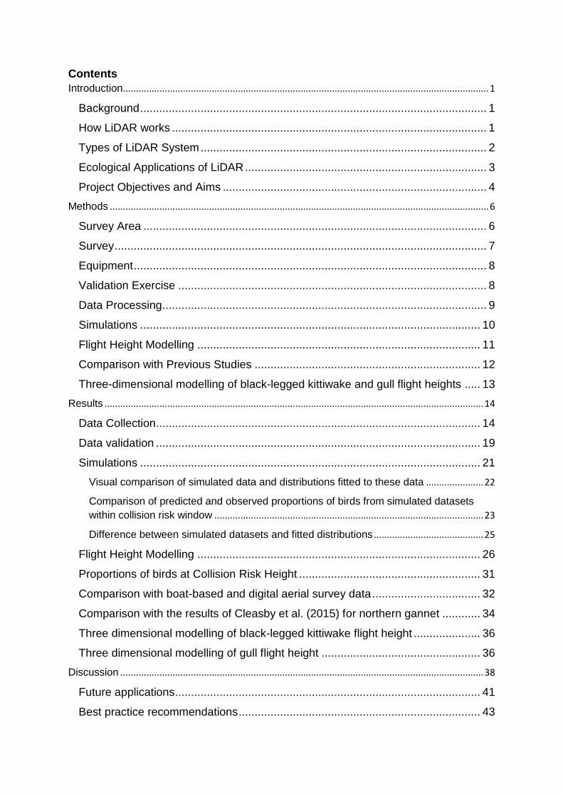
mounted in aircraft, these maps may be combined with high resolution GPS data in
order to create a detailed, geo-referenced point cloud of a surface (Figure 1).
Figure 1: Example point cloud collected using LiDAR showing an area of sea surface in the Outer Forth and Tay Estuaries. The blue colours indicate waves and troughs with darker colours reflecting deeper troughs and lighter colours indicating higher waves. Black indicates areas for which no signal was detected. Note that the black areas are concentrated towards the edges of the image where the beam from the LiDAR will be less focussed. Also note highlighted points which are likely to be birds in flight.
Types of LiDAR System
There are two types of LiDAR system, discrete point return systems and continuous
waveform systems (Lefsky et al., 2002). Discrete point return systems collect
estimates of a limited number of heights by identifying major peaks representing
discrete objects in the return signal of the laser. Such systems have a high laser
repetition rate and a footprint with a small diameter. This enables them to collect a
3
relatively dense distribution of sampled points, making them ideal for detailed
mapping of the ground surface or of canopy topography (Lefsky et al., 2002).
Waveform systems record the height distribution of surfaces by recording the time-
varying intensity of the energy returned by each laser pulse. This enables
information to be collected over larger areas than is possible through the use of point
return systems (Lefsky et al., 2002).
The laser wavelength employed in a particular LiDAR instrument largely determines
its interaction (or lack thereof) with various surface types, and, therefore, dictates
how the 3-D structure of potential habitat is recorded by the sensor. For example,
while near-infrared wavelengths are readily reflected by vegetation and soil (thus
making them useful for recording canopy and ground signals), these same
wavelengths are almost wholly absorbed by water and do not provide enough ‘return’
energy for point detection by the instrument (Lefsky et al., 2002). To map
bathymetric habitat features in marine and freshwater environments, therefore, a
higher energy blue-green laser, which can transmit through water and enable
subsurface point detection is required. Other key factors to consider when selecting
LiDAR equipment include the power of the laser and the size of the receiver aperture
as these will determine the maximum altitude from which data can be collected and,
the width of the swath.
Ecological Applications of LiDAR
LiDAR has been widely used by ecologists for tasks such as fine-scale habitat
mapping or assessing woodland structure and composition (Chust et al., 2008; Hill
and Thomson, 2005; Lefsky et al., 2002; Vierling et al., 2008). However, LiDAR is
also widely applied in fields such as meteorology for tasks such as measuring wind
speeds and locating atmospheric boundary layers (Northend et al., 1966). In these
contexts, the presence of flying animals, like insects, has long been acknowledged
as a potential problem for the data collected. Approaches have been developed to
filter out such data (Lefsky et al., 2002; Martner and Moran, 2001). However, the
potential for such filters to be used to monitor populations of flying species including
insects (Kirkeby et al., 2016), bats (Azmy et al., 2012) and birds (Jansson et al.,
2017) is becoming widely recognised. We describe some applications of LiDAR for
monitoring animals in flight below.
Flying insects are economically important as they may act as pollinators of crops,
crop pests and vectors of zoonotic disease. Consequently, there is growing interest
in monitoring their spatio-temporal distributions. A recent study compared a LiDAR
system and a light trap as methods for monitoring insect populations (Kirkeby et al.,
4
2016). This study demonstrated that LiDAR was capable of recording a greater
number of flying insects than was detected using the light trap and, also that it was
capable of making morphological measurements of the detected insects.
Furthermore, LiDAR may also be sensitive enough to record the wing-beat patterns
of insects, further aiding species identification (Fristrup et al., 2017).
A network of multi-wavelength aerosol LiDAR systems operates across Europe in
order to create a comprehensive database describing the horizontal, vertical and
temporal distribution of aerosols in the atmosphere1. Using data collected from a
LiDAR system installed in Athens, Greece, it was possible to use the characteristics
of the LiDAR signals in order to identify 1735 events likely to have been birds and
the altitudes at which they were recorded (Jansson et al., 2016). The wider network
corresponds well to key migration routes across Europe, leading to calls to use data
collected by the LiDAR system in order to monitor migration patterns (Jansson et al.,
2017).
Information about vertical obstructions, such as power lines, is vital for both military
and commercial flight safety. In order to build a dataset containing information on
vertical obstructions, a recent study developed an algorithm to detect objects above
100 feet (30 m) in altitude that may pose a risk to aircraft (Kohlbrenner et al., 2009).
The data were collected from an aircraft mounted LiDAR system at an altitude of
9,000 feet (2750 m). LiDAR was combined with camera imagery in order to identify
any objects detected. In total, over 4,000 objects were detected and assigned to a
series of altitude categories. Of these, 65 objects were assessed as likely to be
birds in flight either on the basis of the accompanying photograph or, on the basis of
behaviour as recorded by the LiDAR. It should be noted that the purpose of this
study was not to detect birds and, as it filtered out observations below 80 feet, many
are likely to have been missed.
Project Objectives and Aims
Whilst LiDAR may offer the potential to quantify seabird flight heights with high
precision, there is a need for a field trial of the technology in order to understand how
the technology performs in a range of different conditions. For example, as is the
case with RADAR measurements of bird movement patterns, there is the potential
for sea clutter to interfere with the detection of birds close to the sea surface. There
is a need to understand how this may influence estimates of seabird flight height
distributions and quantify any resulting uncertainty. The resulting flight height
1 https://www.earlinet.org/index.php?id=earlinet_homepage

5
distributions could be compared to existing distributions derived from tagging data
(Cleasby et al., 2015), digital aerial survey data (Johnston and Cook, 2016) and
boat-based survey data (Johnston et al., 2014) in order to understand how estimates
may vary between platforms and what consequences there may be for the
consenting process. The wider objectives for this project are:
Test and validate a novel approach for collecting flight height data and provide
best practice recommendations for future survey work;
Collect new bird flight height data for five key breeding seabird features of UK
SPAs (Northern Gannet, Black-legged Kittiwake, Herring Gull, Lesser Black-
backed Gull and Great Black-backed Gull) using a novel application of LiDAR
and digital imagery technology, growing the evidence base;
To use the data collected to model flight height distributions for these five key
species;
To validate flight height estimates collected using LiDAR and digital imagery;
Compare data with those collected using existing methodologies in order to
investigate how different platforms may influence estimates of seabird flight
height, and the uncertainty surrounding estimates of seabird flight height;
Consider how this approach could be used to decrease uncertainty in collision
risk assessments for birds and to reduce uncertainties in the consenting of
offshore wind projects at site-specific and cumulative scales.
6
Methods
Survey Area
The purpose of this work was to test the applicability of LiDAR as a tool for collecting
flight height data and deriving robust flight height distributions suitable for use with
’Option 3’ of the Band Collision Risk Model (Band, 2012). Previous experience with
data from digital aerial surveys suggested that a minimum sample size of 100 birds
is required in order to produce a robust modelled distribution (Johnston and Cook,
2016). Consequently, we reviewed existing datasets including HiDef (2016) and
Stone et al. (1995) in order to identify areas where aerial surveys were likely to
obtain a sufficient sample size for five key species: Northern Gannet Morus
bassanus, Black-legged Kittiwake Rissa tridactyla, Lesser Black-backed Gull Larus
fuscus, Herring Gull Larus argentatus and Great Black-backed Gull Larus marinus.
Based on this review, we identified an area in the Outer Firth of Tay Estuary where
we felt a sufficient sample size could be collected for the five key species. Based on
estimates of the likely speed of the plane and the distribution of the birds within the
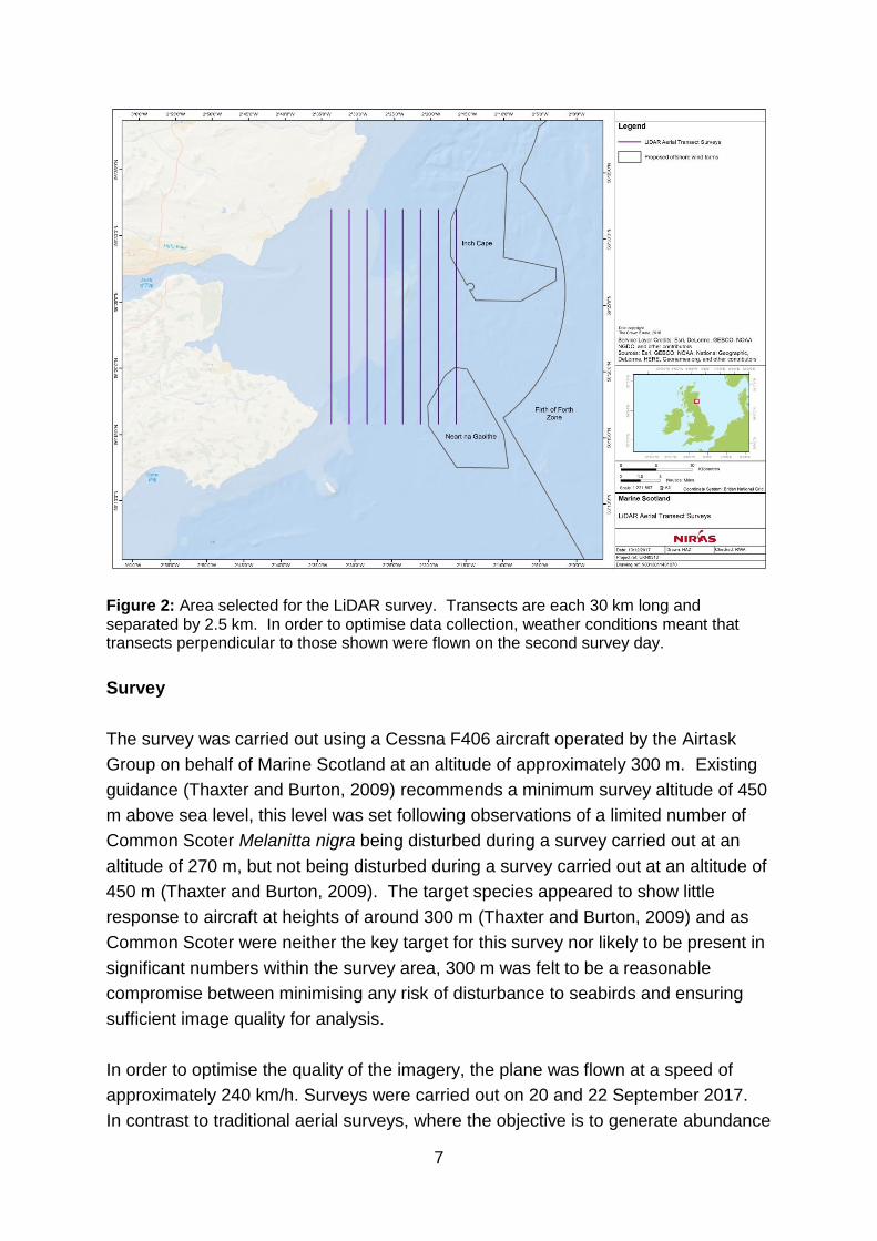
study area, we designed a survey with eight transects, each 30 km long and
separated by 2.5 km (Figure 2). In order to maximise data collection, we aimed to fly
the transects on multiple occasions during the survey period, initially planned for late
July 2017 in order to coincide with the breeding season of the key species at their
colonies in nearby Special Protection Areas (SPAs). Unfortunately, technical issues
lead to the delay of the data collection until the 20-22 September 2017, after the end
of the breeding season for most of the key species. There was a need to maintain a
constant ground speed in order to optimise the quality of the imagery.
Consequently, pilots had the discretion to fly transects perpendicular to those shown
in Figure 2 depending on the prevailing wind conditions for the purposes of the trial
survey.
7
Figure 2: Area selected for the LiDAR survey. Transects are each 30 km long and separated by 2.5 km. In order to optimise data collection, weather conditions meant that transects perpendicular to those shown were flown on the second survey day.
Survey
The survey was carried out using a Cessna F406 aircraft operated by the Airtask
Group on behalf of Marine Scotland at an altitude of approximately 300 m. Existing
guidance (Thaxter and Burton, 2009) recommends a minimum survey altitude of 450
m above sea level, this level was set following observations of a limited number of
Common Scoter Melanitta nigra being disturbed during a survey carried out at an
altitude of 270 m, but not being disturbed during a survey carried out at an altitude of
450 m (Thaxter and Burton, 2009). The target species appeared to show little
response to aircraft at heights of around 300 m (Thaxter and Burton, 2009) and as
Common Scoter were neither the key target for this survey nor likely to be present in
significant numbers within the survey area, 300 m was felt to be a reasonable
compromise between minimising any risk of disturbance to seabirds and ensuring
sufficient image quality for analysis.
In order to optimise the quality of the imagery, the plane was flown at a speed of
approximately 240 km/h. Surveys were carried out on 20 and 22 September 2017.
In contrast to traditional aerial surveys, where the objective is to generate abundance
8
and/or density estimates, the purpose of this survey was to trial a methodology for
collecting flight height information. Consequently, we were not restricted by weather
constraints in the way we would have been had we been collecting abundance data
to generate estimates of population size. On 20 September, the eight transects were
covered once over a period of 1.5 hours. The conditions were overcast with light
wind and no rain, sea conditions were relatively calm. On 22 September, the
surveys were carried out over a period of 4.5 hours, during which time all eight
transects were covered twice and four of the transects were covered a third time.
Conditions during this flight were similar to those recorded during the first although,
wind direction had changed, meaning transects were aligned from east to west
(perpendicular to those shown in Figure 2) in order to optimise flight conditions. A
second survey that day was abandoned after 45 minutes as the light drizzle at the
beginning of the flight turned to heavy rain. For more details about the equipment,
survey site selection and fieldwork, see Appendix 1.
Equipment
To collect data on seabird flight heights, the aircraft was equipped with a Riegl 780i
LiDAR system and a Phase One iXA180 Camera. The camera was set with a 1.6
seconds repetition rate, enabling a 60% spatial overlap between images, provided
associated imagery to identify individual birds to species level. The Riegl 780i
LiDAR is a near-infrared waveform system with a high laser pulse repetition rate of
up to 1 MHz. This reflected a need to collect data from across a relatively broad
area above the sea-surface. From an altitude of 300 m above sea level, the LiDAR
had a point density of approximately 11 points m-2 on the sea surface and a swath of
approximately 300 m. The camera had a Ground Sample Distance of approximately
3.5 cm and a swath of approximately 350 m.
Validation Exercise
The initial validation exercise was planned to coincide with the main data collection.
However, adverse weather conditions meant that it was not possible to carry out this
work as planned. Consequently, the validation exercise was re-arranged and carried
out on the western coast of Zealand in Denmark on 6 April 2018. The aircraft and
equipment for this validation exercise were set up so as to minimise any differences
with the main study in order to ensure that the results were transferable.
Three drones were flown simultaneously at heights of approximately 10 m, 40 m and
80 m above sea level. The drones were then overflown by an aircraft equipped with
a Riegl 480i LiDAR scanner (which has a similar specification to the Riegl 780 LiDAR
9
used for the main study). As with the main survey, the plane flew at an altitude of
approximately 300 m above sea-level and at a speed of approximately 240 km h-1.
This gave a point density of approximately 10 points m-2 at ground level. The drones
were overflown seven times. On four occasions the drones were stationary and on
three occasions the drones were moving at speeds of 7-15 km h-1, taken as
representative of seabird flight speed (Alerstam et al., 2007). The height of each
drone was then estimated using on board GPS, LiDAR and photogrammetry based
on overlap of the images from the drones and the presence of marked control points
of known height. For more details of the validation exercise, see Appendix 1.
Data Processing
Initially, the internal geometry (angle and distance to points) of the LiDAR dataset
was analysed in order to isolate single points, or groups of points, that could be the
reflections of birds in flight. In order to estimate flight height, points which were
classified as birds were compared to those which were classified as sea. The height
of each point in the LiDAR cloud was measured in relation to the European
Terrestrial Reference System 89 (ETRS89), the EU recommended frame of
reference for European geo-data. Flight height estimates made using traditional
digital aerial surveys are based on calculations made in relation to the altitude of the
survey aircraft (Thaxter et al., 2016). Where there is error associated with the
estimation of the altitude of the survey aircraft, this is introduced into the estimation
of seabird flight height. Flight height estimates made using LiDAR are made in
relation to the position of the sea surface, generating a precise measurement of
seabird height above sea-level which was independent of the height of the survey
aircraft. The flight speed of the plane meant that any individual bird could not be
captured by more than one set of LiDAR points.
As is the case with RADAR, sea-swell may interfere with estimates of seabird flight
height resulting in too many false positive records of seabird flight heights for the
data to be reliable. Consequently, a minimum height threshold was set in order to
ensure that the resulting dataset did not contain too many false positive estimates of
seabird flight heights. This minimum threshold varied in relation to weather
conditions. In calmer conditions on 20 September 2017, it was possible to lower this
threshold to 1 m above sea level, for the first survey on 22 September a threshold of
1.5 m above sea level was possible and, as weather conditions worsened, for the
second survey on 22 September, a threshold of 2 m above sea level was possible.
Having identified potential birds within the LiDAR point cloud, the average position of
each set of points (height, latitude and longitude) was determined based on the
10
angle and time taken for each LiDAR pulse to return to the LiDAR system. This
information was then used to pinpoint the location of the bird in photographs taken
before and after the LiDAR pulse. The LiDAR equipment and the camera were both
attached to an Inertial Measurement Unit (IMU) on board the aircraft. The IMU
precisely measures acceleration in three directions to survey grade accuracy. This
meant that the images from the camera could be matched to the information from the
LiDAR with a high degree of accuracy.
The photographs were then passed to an ornithologist for identification. In order to
help identify which bird the LiDAR record related to in instances where two or more
birds occurred on the same photographs, the LiDAR point(s) were projected onto the
image. No points above the minimum thresholds were identified as anything other
than birds.
Simulations
Approaches such as kernel density plots are a relatively simple and straightforward
way of describing the underlying distributions of data such as the estimates of flight
height collected as part of this study. However, such an approach is likely to result in
a flight height distribution which is over-fitted to the underlying data. The data
collected during this study were samples from the true flight height distributions of
the species using the study area. A kernel density plot would describe this sample
exactly, but may not be an accurate representation of the true underlying distribution.
To describe the true, underlying distribution, we attempted to fit the data using a pre-
defined distributional form (Johnston and Cook, 2016). However, in order to do this,
it was important to identify a distribution that was sufficiently flexible to describe a
broad range of data. This helped to ensure that we were able to describe the
underlying flight height distribution, rather than just the sample that we have
collected from that distribution.
In order to achieve this, we simulated datasets informed by the survey data in which
the underlying distribution was either a normal, log-normal, gamma, normal-mixture
or gamma-mixture distribution using the mixtools (Benaglia et al., 2009) and
fitdistrplus (Delignette-Muller and Dutang, 2015) packages in the R statistical
package (R Core Team, 2014). We then attempted to fit each distribution to each
simulated dataset in turn. In order to determine how sample size influenced the
ability to fit distributions to data we considered samples of 10, 25, 50, 75, 100, 150
and 200 individuals from each simulated dataset. For each underlying distribution
and each sample size, we repeated this process 1,000 times.
11
Following Johnston & Cook (2016) we assessed how well each distribution fitted the
simulated datasets in three ways:
1. Visual comparison of the fitted distributions and the simulated datasets they
were derived from;
2. Comparison of the predicted and observed proportions of birds from simulated
datasets within a 20-120 m collision risk window (as defined in Johnston et al.,
2014);
3. Assessment of the difference between fitted distributions and the simulated
datasets summed in 10 m height bands (0-10 m, 10-20 m, etc.).
Flight Height Modelling
We used the outcome of the simulation exercise in order to determine which
distribution best fitted the data. Initially, we produced flight height distributions based
on data from all three surveys. However, the minimum threshold above which flight
height data was collected varied from 1-2 m above sea level. Therefore, to ensure
consistency between surveys, we only considered records of birds that were a
minimum of 2 m above sea level when we modelled the full dataset.
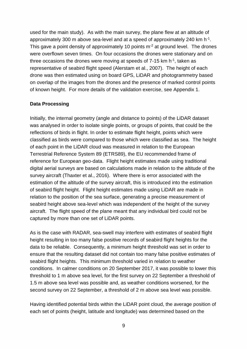
The survey aircraft may be thought of as being at the tip of a pyramid (Figure 3). As
both the LiDAR points and the digital imagery originate from this point, towards the
edge of the survey transects, the probability of detecting a bird in flight will decline as
its flight height increases. This may lead to the modelled flight height distributions
being negatively biased. In order to test this, we used basic trigonometry to
calculate the horizontal distance of each bird from the survey aircraft. We then
compared modelled distributions and the proportion of birds estimated to be at
collision risk height for all birds, birds within 150 m of the survey aircraft horizontally,
birds within 125 m of the survey aircraft and birds within 100 m of the aircraft. This
analysis was used to determine the optimal horizontal distance from the survey
aircraft with which to produce the final modelled distribution. We then compared this
distribution to distributions based on each individual survey. Comparison of
modelled distributions from the first and third surveys also enabled us to understand
the implications of excluding birds with a flight height of 1-2 m from the final analysis.
12
Figure 3: The LiDAR and camera system are within an aircraft which is effectively at the tip of a pyramid, meaning that towards the edges of the survey transect, the probability of detecting a bird in flight varies with the height at which that bird flies.
Comparison with Previous Studies
Flight height data have previously been collected using boat-based surveys, digital
aerial surveys and tagging data (Cleasby et al., 2015; Johnston et al., 2014;
Johnston and Cook, 2016). For boat-based surveys and digital aerial surveys, data
were used to derive continuous flight height distributions. We compared the flight
height distributions derived from the LiDAR data to those derived in these previous
studies (Johnston et al., 2014; Johnston and Cook, 2016).
Cleasby et al. (2015) collected flight height data from 16 northern gannets fitted with
GPS tags and altimeters in the Outer Forth and Tay Estuaries between mid-June
and mid-August 2010 and 2011. They modelled flight heights, as measured using
the altimeters, using a Generalized Additive Mixed Model (Wood, 2006) which
included an isotropic smooth of latitude and longitude, enabling spatial predictions of
flight height. Trip number nested within bird identity was included as a random
effect. Although the studies did not overlap in time, the study area considered by
Cleasby et al. (2015) encompassed that covered by the present LiDAR study. To
enable comparison with the spatial patterns in flight heights obtained from altimeters
by Cleasby et al. (2015), we, therefore, used a similar modelling approach to also
explore spatial patterns in flight heights of northern gannets, as recorded by LiDAR
in the present study. We modelled flight height data collected using LiDAR using a
13
Generalized Additive Model (Wood, 2006) again with an isotropic smooth of latitude
and longitude.
Three-Dimensional Modelling of Black-Legged Kittiwake and Gull Flight
Heights
Following the approach described above for northern gannet, we also applied the
same approach to model spatial patterns in the flight heights of black-legged
kittiwakes and other gulls within the study area. We again modelled the flight height
data collected using LiDAR using a Generalized Additive Model with an isotropic
smooth of latitude and longitude, enabling spatial patterns in flight heights to be
examined.
14
Results
Data Collection
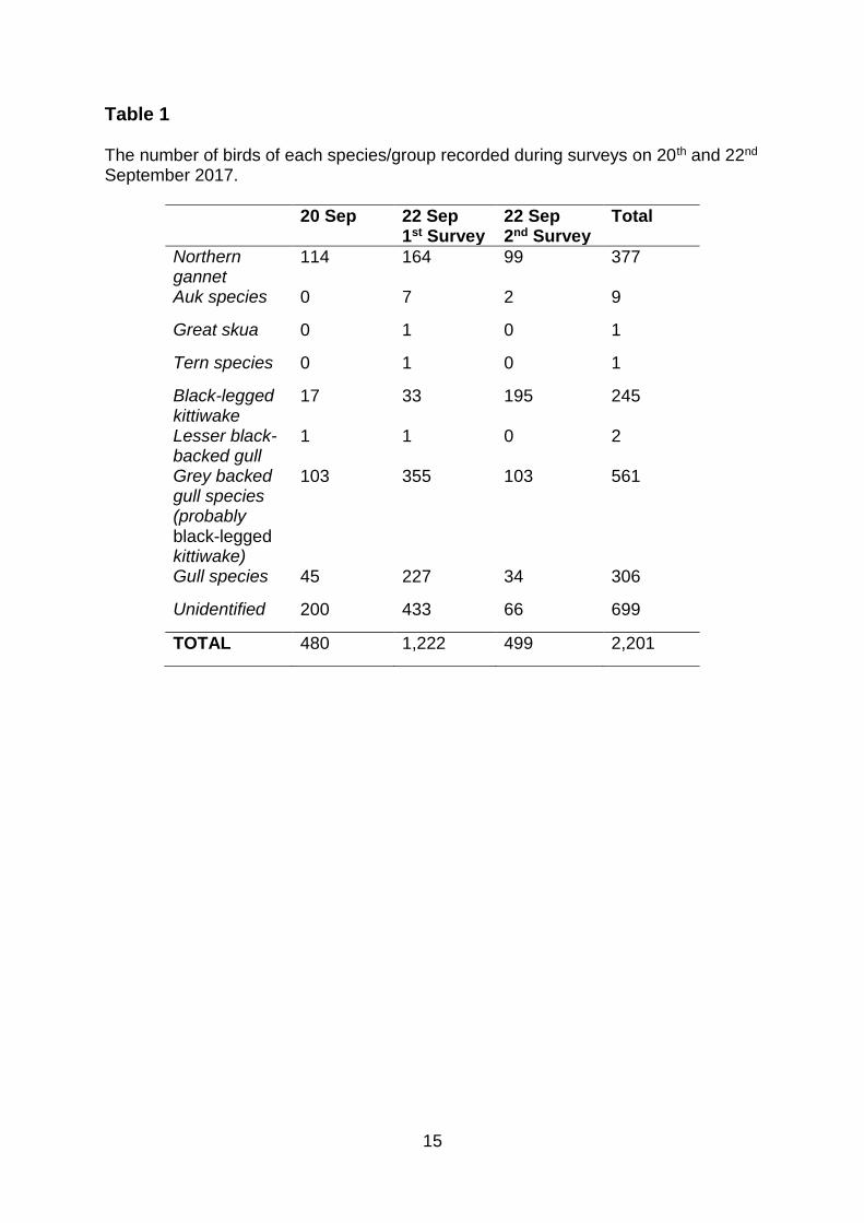
A total of 2,487 LiDAR clusters were identified as potentially containing birds. Of
these, on closer inspection, birds could not be found in the photographs relating to
286 (11%) of these records. These clusters consisted of less than four LiDAR points
and are considered to most likely relate to suspended matter in the air. The most
abundant identified species were northern gannet and black-legged kittiwake (Table
1). A large number of grey-backed gull species were also identified in the imagery.
Given the location and the time of year, it is almost certain that these were black-
legged kittiwake (HiDef, 2016) and they were treated as such in subsequent
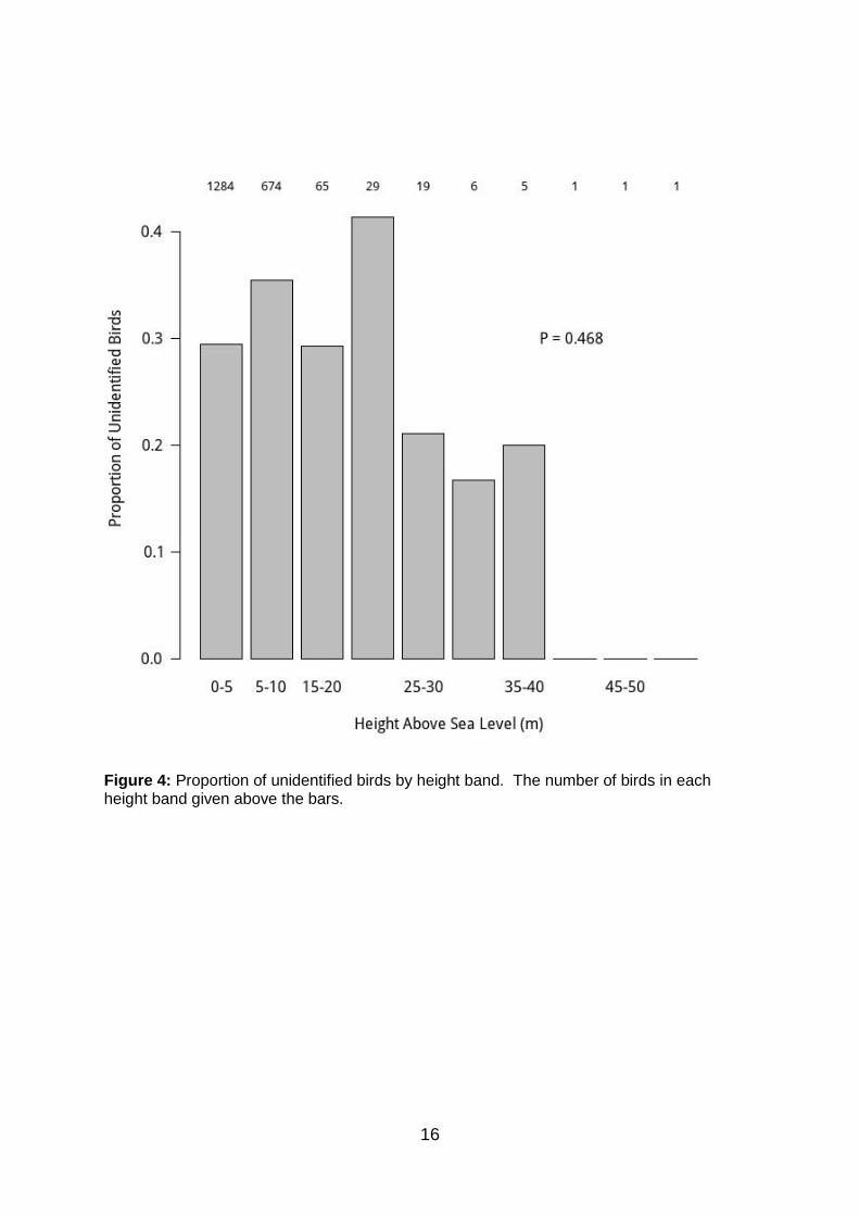
analyses. The data also included records of a large number of unidentified birds.
This was the result of a technical issue causing equipment vibration and meant that
the image resolution was too poor to allow species identification. If the unidentified
birds were not randomly distributed in relation to height above sea level, this had the
potential to bias any modelled flight height distribution. However, analyses of these
data using a Generalised Linear Model with a binomial error structure (identified/not
identified) (Figure 4), suggested that the proportion of unidentified birds did not vary
in relation to flight height.
15
Table 1 The number of birds of each species/group recorded during surveys on 20th and 22nd September 2017.
20 Sep 22 Sep 1st Survey
22 Sep 2nd Survey
Total
Northern gannet
114 164 99 377
Auk species 0 7 2 9
Great skua 0 1 0 1
Tern species 0 1 0 1
Black-legged kittiwake
17 33 195 245
Lesser black-backed gull
1 1 0 2
Grey backed gull species (probably black-legged kittiwake)
103 355 103 561
Gull species 45 227 34 306
Unidentified 200 433 66 699
TOTAL 480 1,222 499 2,201
16
Figure 4: Proportion of unidentified birds by height band. The number of birds in each height band given above the bars.
17
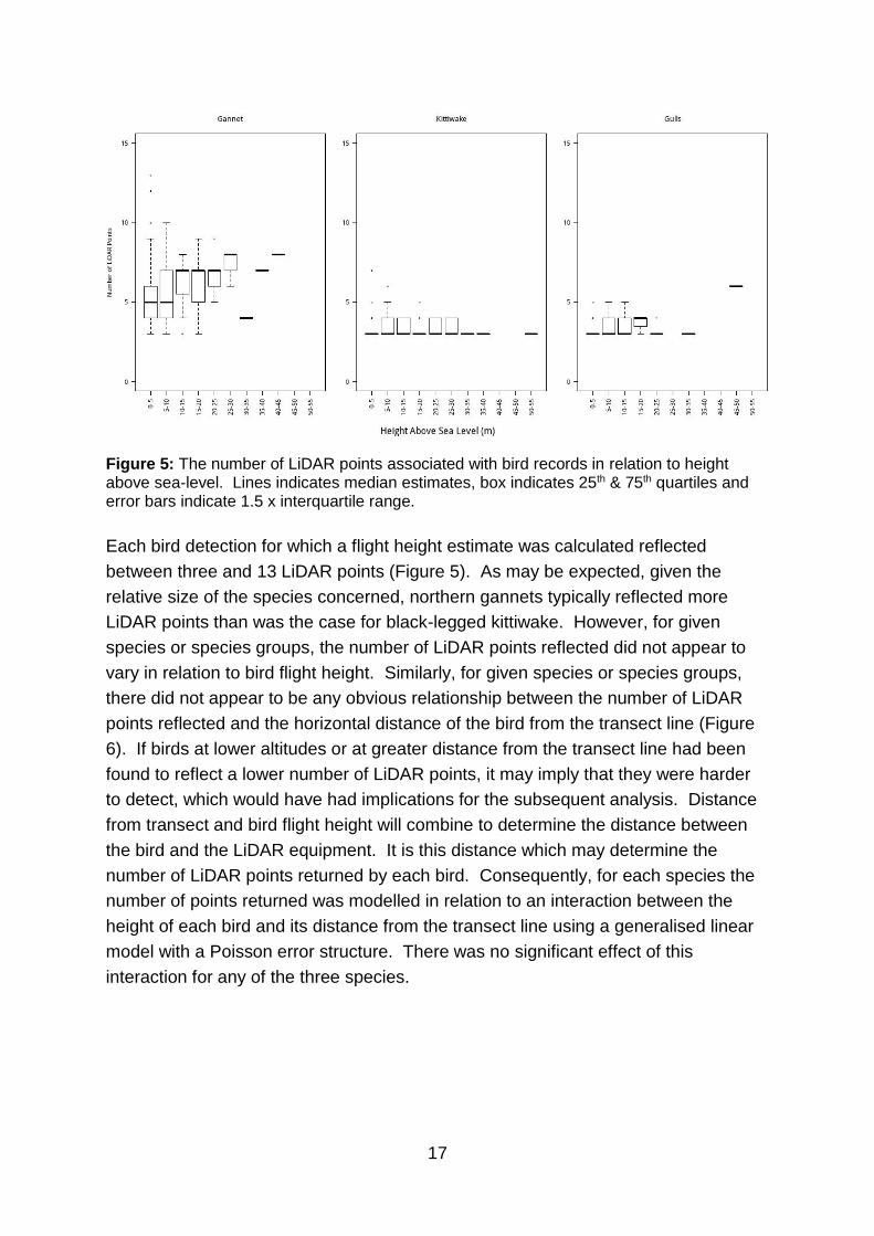
Figure 5: The number of LiDAR points associated with bird records in relation to height above sea-level. Lines indicates median estimates, box indicates 25th & 75th quartiles and error bars indicate 1.5 x interquartile range.
Each bird detection for which a flight height estimate was calculated reflected
between three and 13 LiDAR points (Figure 5). As may be expected, given the
relative size of the species concerned, northern gannets typically reflected more
LiDAR points than was the case for black-legged kittiwake. However, for given
species or species groups, the number of LiDAR points reflected did not appear to
vary in relation to bird flight height. Similarly, for given species or species groups,
there did not appear to be any obvious relationship between the number of LiDAR
points reflected and the horizontal distance of the bird from the transect line (Figure
6). If birds at lower altitudes or at greater distance from the transect line had been
found to reflect a lower number of LiDAR points, it may imply that they were harder
to detect, which would have had implications for the subsequent analysis. Distance
from transect and bird flight height will combine to determine the distance between
the bird and the LiDAR equipment. It is this distance which may determine the
number of LiDAR points returned by each bird. Consequently, for each species the
number of points returned was modelled in relation to an interaction between the
height of each bird and its distance from the transect line using a generalised linear
model with a Poisson error structure. There was no significant effect of this
interaction for any of the three species.
18
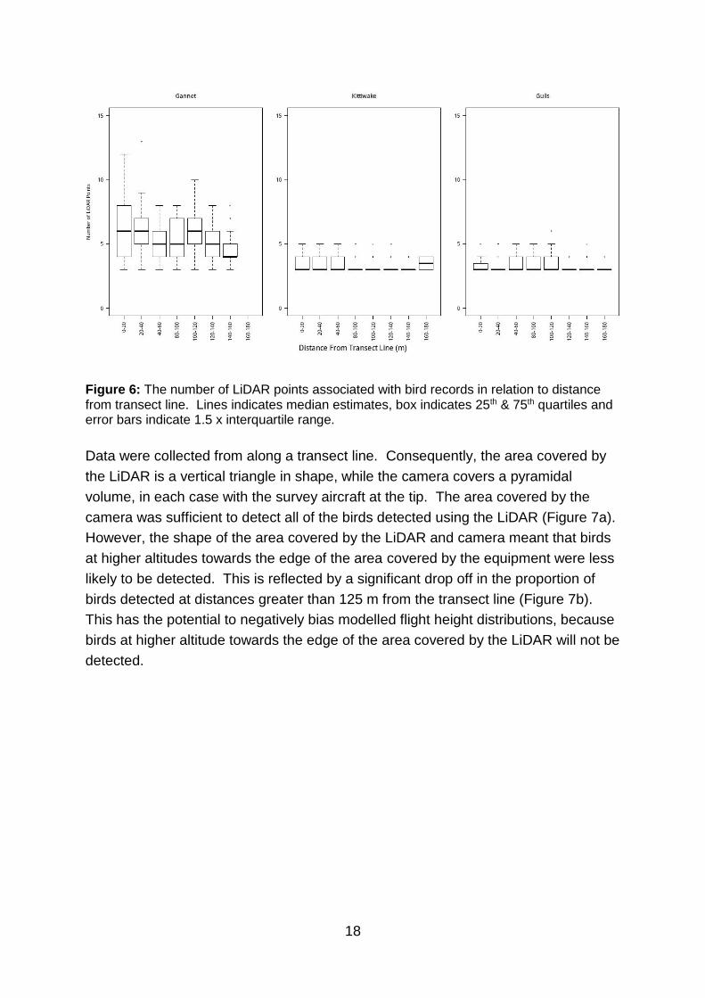
Figure 6: The number of LiDAR points associated with bird records in relation to distance from transect line. Lines indicates median estimates, box indicates 25th & 75th quartiles and error bars indicate 1.5 x interquartile range.
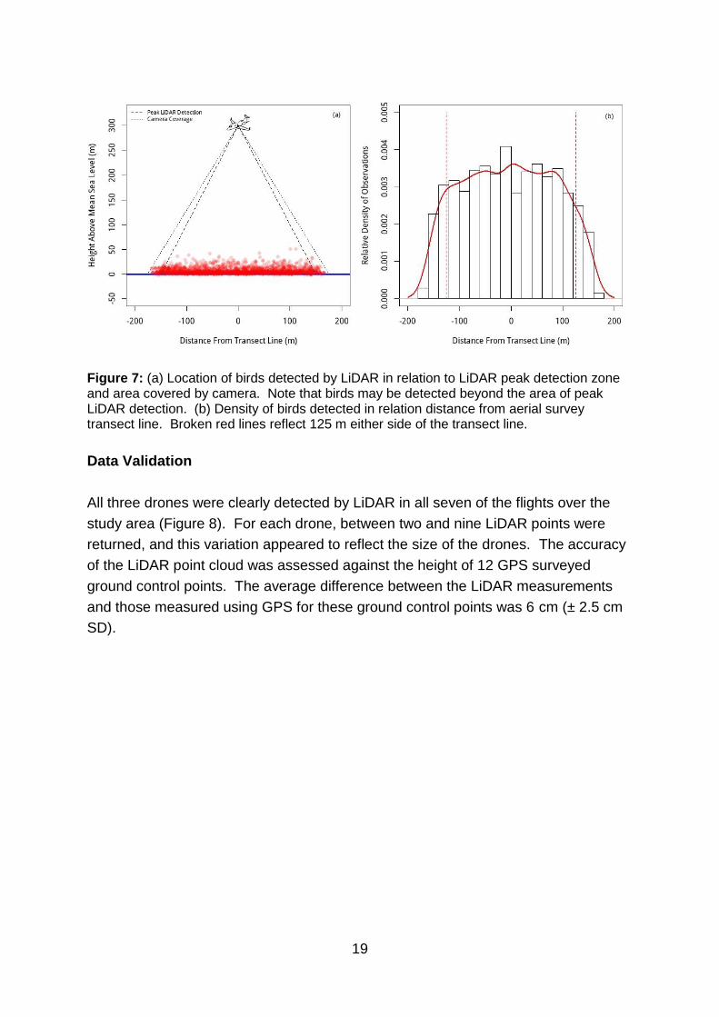
Data were collected from along a transect line. Consequently, the area covered by
the LiDAR is a vertical triangle in shape, while the camera covers a pyramidal
volume, in each case with the survey aircraft at the tip. The area covered by the
camera was sufficient to detect all of the birds detected using the LiDAR (Figure 7a).
However, the shape of the area covered by the LiDAR and camera meant that birds
at higher altitudes towards the edge of the area covered by the equipment were less
likely to be detected. This is reflected by a significant drop off in the proportion of
birds detected at distances greater than 125 m from the transect line (Figure 7b).
This has the potential to negatively bias modelled flight height distributions, because
birds at higher altitude towards the edge of the area covered by the LiDAR will not be
detected.
19
Figure 7: (a) Location of birds detected by LiDAR in relation to LiDAR peak detection zone and area covered by camera. Note that birds may be detected beyond the area of peak LiDAR detection. (b) Density of birds detected in relation distance from aerial survey transect line. Broken red lines reflect 125 m either side of the transect line.
Data Validation
All three drones were clearly detected by LiDAR in all seven of the flights over the
study area (Figure 8). For each drone, between two and nine LiDAR points were
returned, and this variation appeared to reflect the size of the drones. The accuracy
of the LiDAR point cloud was assessed against the height of 12 GPS surveyed
ground control points. The average difference between the LiDAR measurements
and those measured using GPS for these ground control points was 6 cm (± 2.5 cm
SD).
20
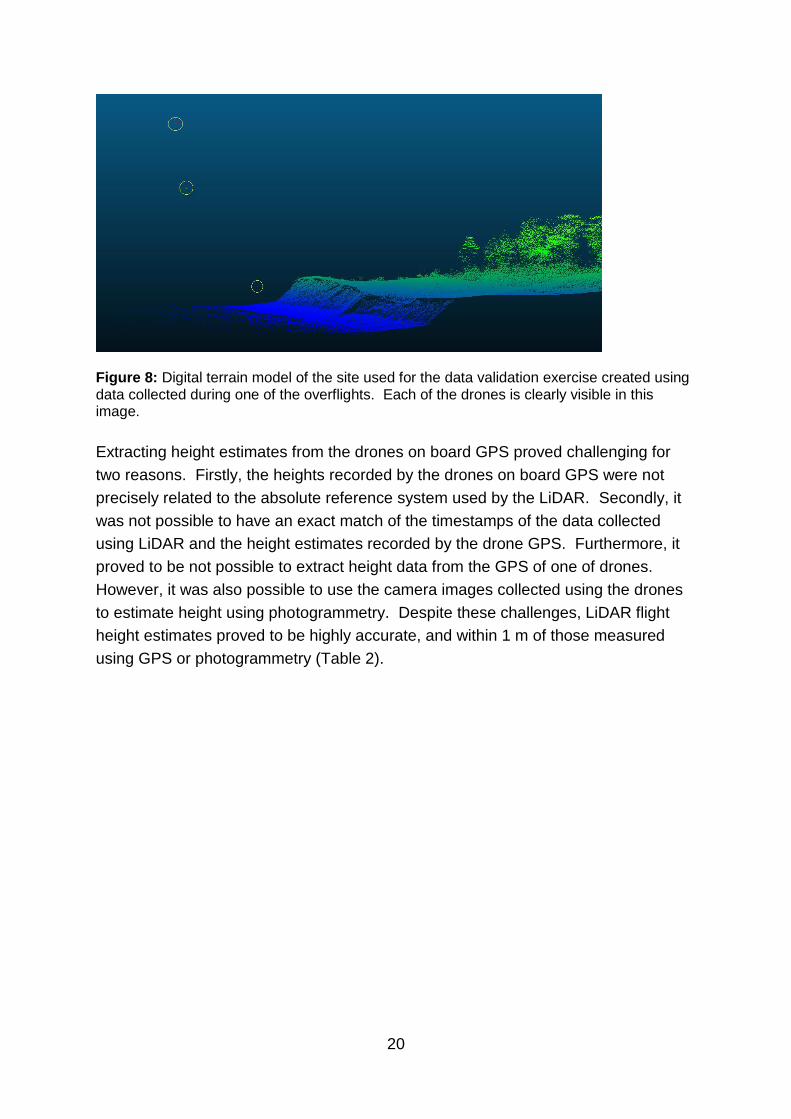
Figure 8: Digital terrain model of the site used for the data validation exercise created using data collected during one of the overflights. Each of the drones is clearly visible in this image.
Extracting height estimates from the drones on board GPS proved challenging for
two reasons. Firstly, the heights recorded by the drones on board GPS were not
precisely related to the absolute reference system used by the LiDAR. Secondly, it
was not possible to have an exact match of the timestamps of the data collected
using LiDAR and the height estimates recorded by the drone GPS. Furthermore, it
proved to be not possible to extract height data from the GPS of one of drones.
However, it was also possible to use the camera images collected using the drones
to estimate height using photogrammetry. Despite these challenges, LiDAR flight
height estimates proved to be highly accurate, and within 1 m of those measured
using GPS or photogrammetry (Table 2).
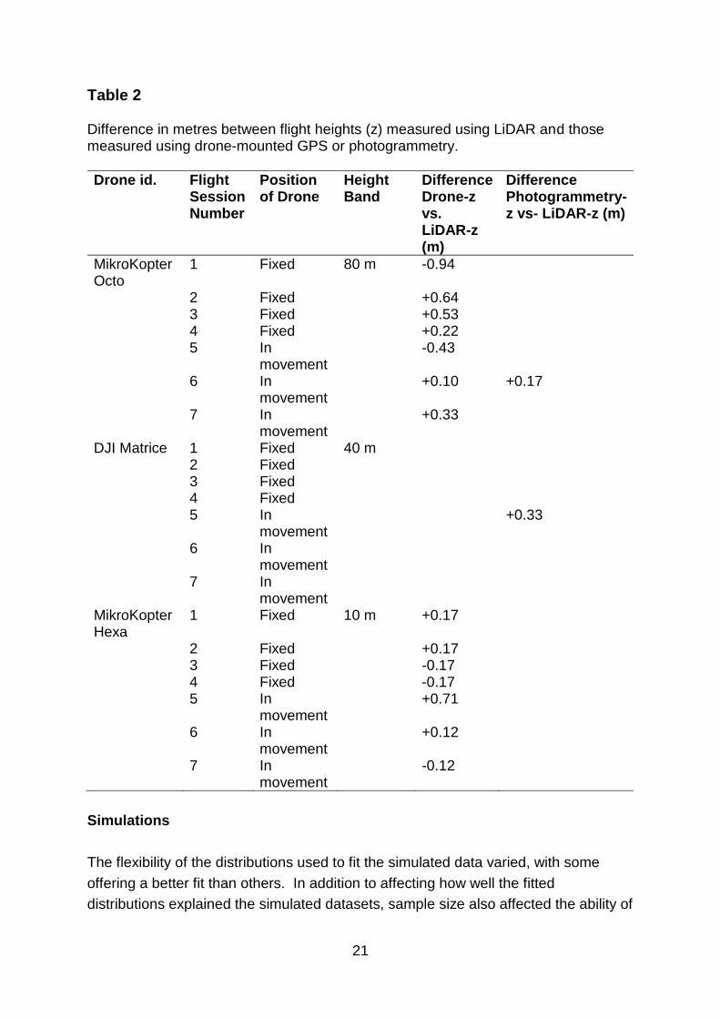
21
Table 2 Difference in metres between flight heights (z) measured using LiDAR and those measured using drone-mounted GPS or photogrammetry.
Drone id. Flight Session Number
Position of Drone
Height Band
Difference Drone-z vs. LiDAR-z (m)
Difference Photogrammetry-z vs- LiDAR-z (m)
MikroKopter Octo
1 Fixed 80 m -0.94
2 Fixed +0.64 3 Fixed +0.53 4 Fixed +0.22 5 In
movement -0.43
6 In movement
+0.10 +0.17
7 In movement
+0.33
DJI Matrice 1 Fixed 40 m 2 Fixed 3 Fixed 4 Fixed 5 In
movement +0.33
6 In movement
7 In movement
MikroKopter Hexa
1 Fixed 10 m +0.17
2 Fixed +0.17 3 Fixed -0.17 4 Fixed -0.17 5 In
movement +0.71
6 In movement
+0.12
7 In movement
-0.12
Simulations
The flexibility of the distributions used to fit the simulated data varied, with some
offering a better fit than others. In addition to affecting how well the fitted
distributions explained the simulated datasets, sample size also affected the ability of
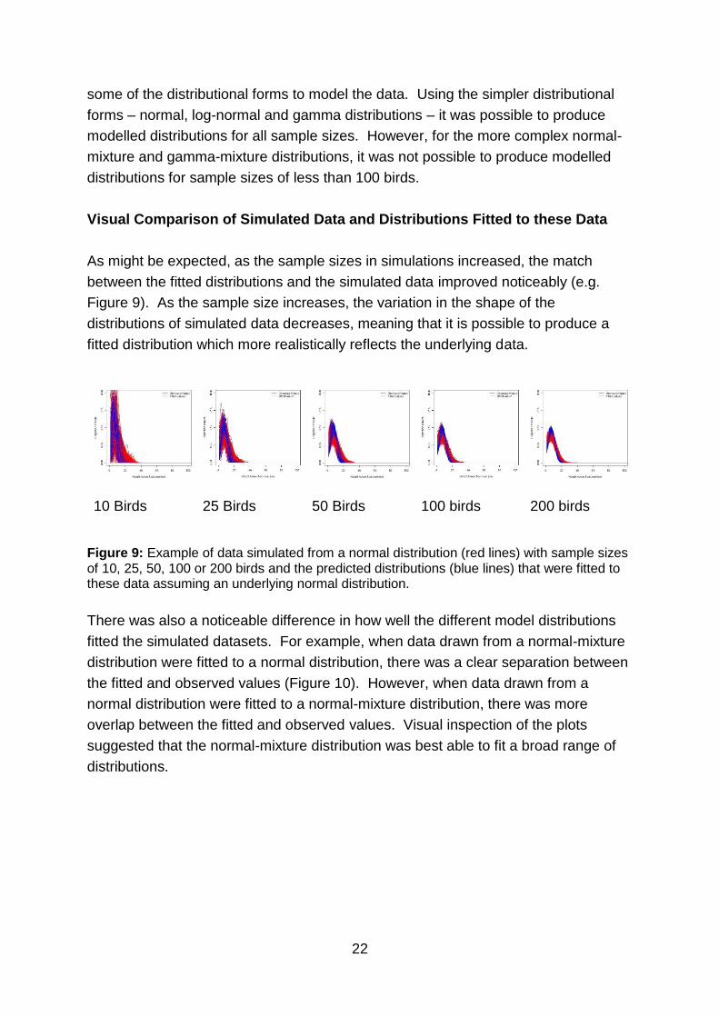
22
some of the distributional forms to model the data. Using the simpler distributional
forms – normal, log-normal and gamma distributions – it was possible to produce
modelled distributions for all sample sizes. However, for the more complex normal-
mixture and gamma-mixture distributions, it was not possible to produce modelled
distributions for sample sizes of less than 100 birds.
Visual Comparison of Simulated Data and Distributions Fitted to these Data
As might be expected, as the sample sizes in simulations increased, the match
between the fitted distributions and the simulated data improved noticeably (e.g.
Figure 9). As the sample size increases, the variation in the shape of the
distributions of simulated data decreases, meaning that it is possible to produce a
fitted distribution which more realistically reflects the underlying data.
10 Birds 25 Birds 50 Birds 100 birds 200 birds
Figure 9: Example of data simulated from a normal distribution (red lines) with sample sizes of 10, 25, 50, 100 or 200 birds and the predicted distributions (blue lines) that were fitted to these data assuming an underlying normal distribution.
There was also a noticeable difference in how well the different model distributions
fitted the simulated datasets. For example, when data drawn from a normal-mixture
distribution were fitted to a normal distribution, there was a clear separation between
the fitted and observed values (Figure 10). However, when data drawn from a
normal distribution were fitted to a normal-mixture distribution, there was more
overlap between the fitted and observed values. Visual inspection of the plots
suggested that the normal-mixture distribution was best able to fit a broad range of
distributions.
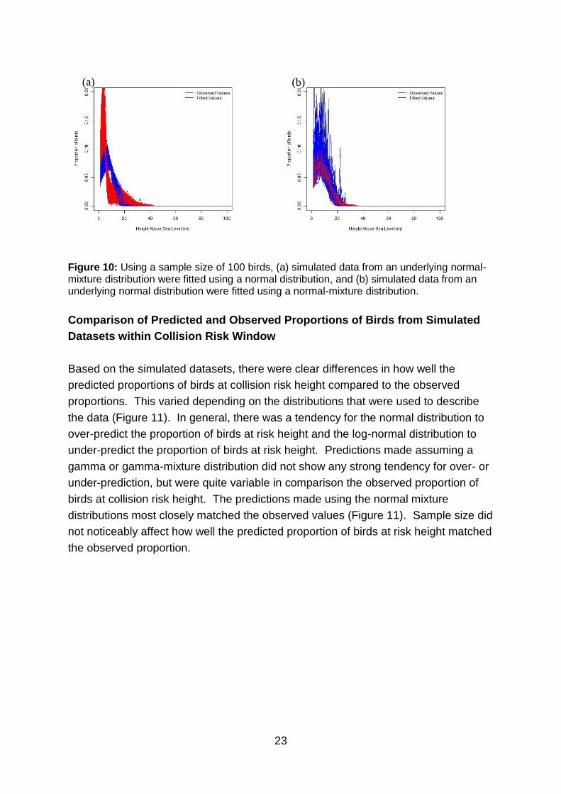
23
Figure 10: Using a sample size of 100 birds, (a) simulated data from an underlying normal-mixture distribution were fitted using a normal distribution, and (b) simulated data from an underlying normal distribution were fitted using a normal-mixture distribution.
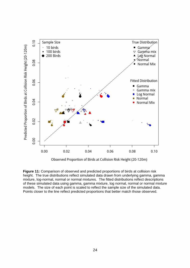
Comparison of Predicted and Observed Proportions of Birds from Simulated
Datasets within Collision Risk Window
Based on the simulated datasets, there were clear differences in how well the
predicted proportions of birds at collision risk height compared to the observed
proportions. This varied depending on the distributions that were used to describe
the data (Figure 11). In general, there was a tendency for the normal distribution to
over-predict the proportion of birds at risk height and the log-normal distribution to
under-predict the proportion of birds at risk height. Predictions made assuming a
gamma or gamma-mixture distribution did not show any strong tendency for over- or
under-prediction, but were quite variable in comparison the observed proportion of
birds at collision risk height. The predictions made using the normal mixture
distributions most closely matched the observed values (Figure 11). Sample size did
not noticeably affect how well the predicted proportion of birds at risk height matched
the observed proportion.
(a) (b)
24
Figure 11: Comparison of observed and predicted proportions of birds at collision risk height. The true distributions reflect simulated data drawn from underlying gamma, gamma mixture, log-normal, normal or normal mixtures. The fitted distributions reflect descriptions of these simulated data using gamma, gamma mixture, log normal, normal or normal mixture models. The size of each point is scaled to reflect the sample size of the simulated data. Points closer to the line reflect predicted proportions that better match those observed.
25
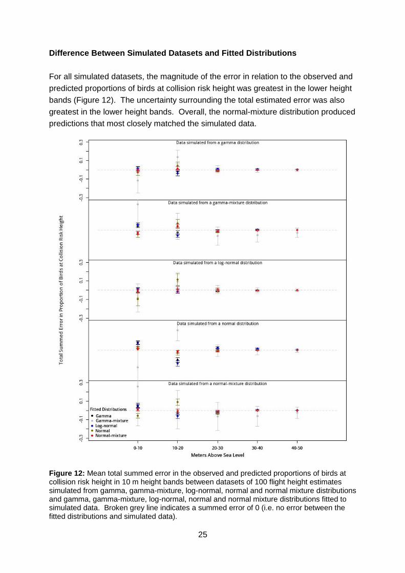
Difference Between Simulated Datasets and Fitted Distributions
For all simulated datasets, the magnitude of the error in relation to the observed and
predicted proportions of birds at collision risk height was greatest in the lower height
bands (Figure 12). The uncertainty surrounding the total estimated error was also
greatest in the lower height bands. Overall, the normal-mixture distribution produced
predictions that most closely matched the simulated data.
Figure 12: Mean total summed error in the observed and predicted proportions of birds at collision risk height in 10 m height bands between datasets of 100 flight height estimates simulated from gamma, gamma-mixture, log-normal, normal and normal mixture distributions and gamma, gamma-mixture, log-normal, normal and normal mixture distributions fitted to simulated data. Broken grey line indicates a summed error of 0 (i.e. no error between the fitted distributions and simulated data).
26
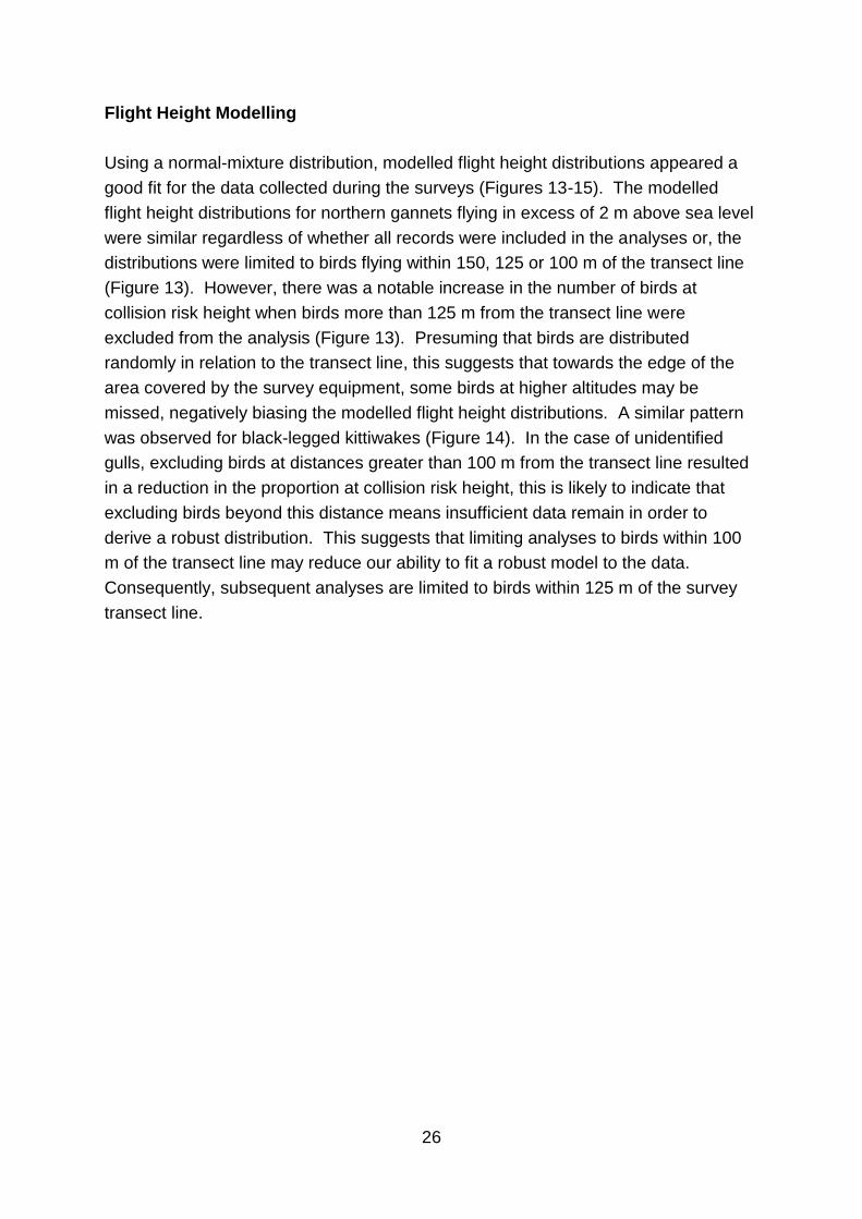
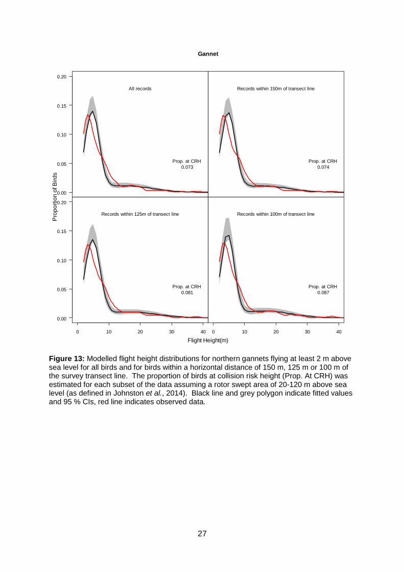
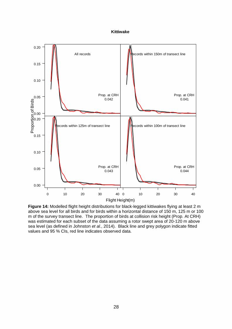
Flight Height Modelling
Using a normal-mixture distribution, modelled flight height distributions appeared a
good fit for the data collected during the surveys (Figures 13-15). The modelled
flight height distributions for northern gannets flying in excess of 2 m above sea level
were similar regardless of whether all records were included in the analyses or, the
distributions were limited to birds flying within 150, 125 or 100 m of the transect line
(Figure 13). However, there was a notable increase in the number of birds at
collision risk height when birds more than 125 m from the transect line were
excluded from the analysis (Figure 13). Presuming that birds are distributed
randomly in relation to the transect line, this suggests that towards the edge of the
area covered by the survey equipment, some birds at higher altitudes may be
missed, negatively biasing the modelled flight height distributions. A similar pattern
was observed for black-legged kittiwakes (Figure 14). In the case of unidentified
gulls, excluding birds at distances greater than 100 m from the transect line resulted
in a reduction in the proportion at collision risk height, this is likely to indicate that
excluding birds beyond this distance means insufficient data remain in order to
derive a robust distribution. This suggests that limiting analyses to birds within 100
m of the transect line may reduce our ability to fit a robust model to the data.
Consequently, subsequent analyses are limited to birds within 125 m of the survey
transect line.
27
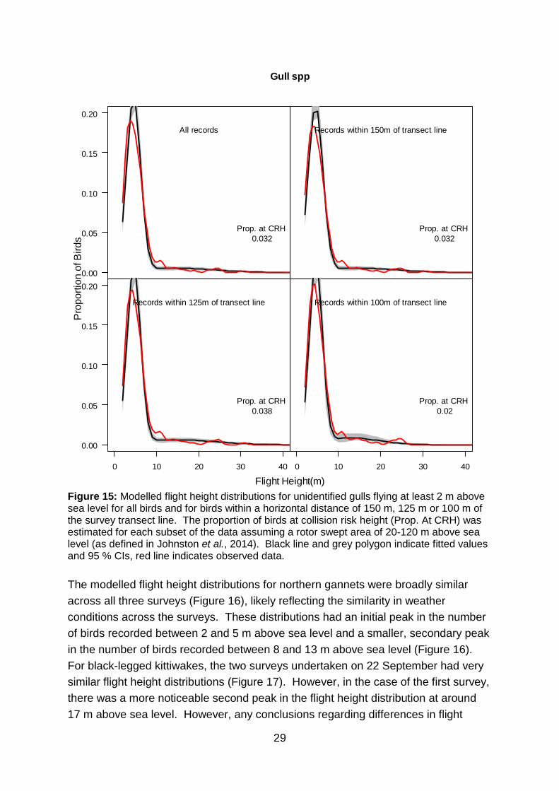
Figure 13: Modelled flight height distributions for northern gannets flying at least 2 m above sea level for all birds and for birds within a horizontal distance of 150 m, 125 m or 100 m of the survey transect line. The proportion of birds at collision risk height (Prop. At CRH) was estimated for each subset of the data assuming a rotor swept area of 20-120 m above sea level (as defined in Johnston et al., 2014). Black line and grey polygon indicate fitted values and 95 % CIs, red line indicates observed data.
0.00
0.05
0.10
0.15
0.20
All records
Prop. at CRH
0.073
Records within 150m of transect line
Prop. at CRH
0.074
0 10 20 30 40
0.00
0.05
0.10
0.15
0.20
Records within 125m of transect line
Prop. at CRH
0.081
0 10 20 30 40
Records within 100m of transect line
Prop. at CRH
0.087
Flight Height(m)
Pro
po
rtio
n o
f B
ird
sGannet
28
Figure 14: Modelled flight height distributions for black-legged kittiwakes flying at least 2 m above sea level for all birds and for birds within a horizontal distance of 150 m, 125 m or 100 m of the survey transect line. The proportion of birds at collision risk height (Prop. At CRH) was estimated for each subset of the data assuming a rotor swept area of 20-120 m above sea level (as defined in Johnston et al., 2014). Black line and grey polygon indicate fitted values and 95 % CIs, red line indicates observed data.
0.00
0.05
0.10
0.15
0.20
All records
Prop. at CRH
0.042
Records within 150m of transect line
Prop. at CRH
0.041
0 10 20 30 40
0.00
0.05
0.10
0.15
0.20
Records within 125m of transect line
Prop. at CRH
0.043
0 10 20 30 40
Records within 100m of transect line
Prop. at CRH
0.044
Flight Height(m)
Pro
po
rtio
n o
f B
ird
sKittiwake
29
Figure 15: Modelled flight height distributions for unidentified gulls flying at least 2 m above sea level for all birds and for birds within a horizontal distance of 150 m, 125 m or 100 m of the survey transect line. The proportion of birds at collision risk height (Prop. At CRH) was estimated for each subset of the data assuming a rotor swept area of 20-120 m above sea level (as defined in Johnston et al., 2014). Black line and grey polygon indicate fitted values and 95 % CIs, red line indicates observed data.
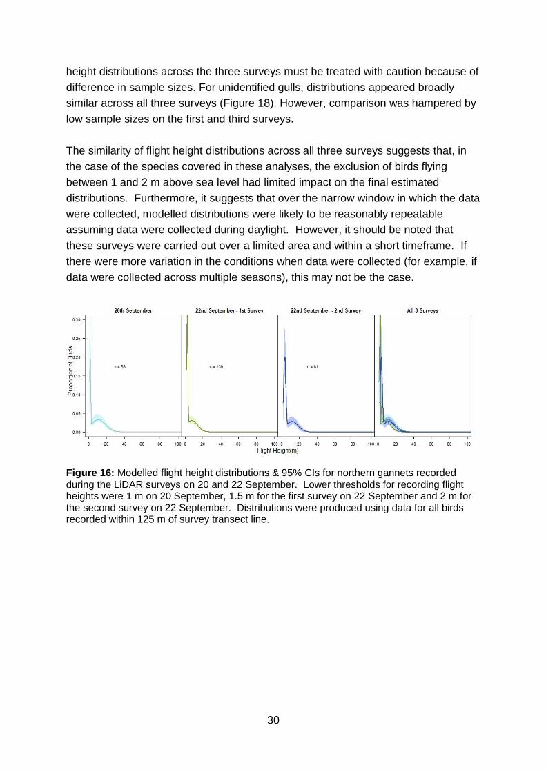
The modelled flight height distributions for northern gannets were broadly similar
across all three surveys (Figure 16), likely reflecting the similarity in weather
conditions across the surveys. These distributions had an initial peak in the number
of birds recorded between 2 and 5 m above sea level and a smaller, secondary peak
in the number of birds recorded between 8 and 13 m above sea level (Figure 16).
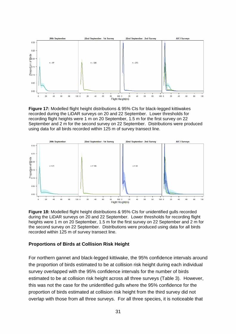
For black-legged kittiwakes, the two surveys undertaken on 22 September had very
similar flight height distributions (Figure 17). However, in the case of the first survey,
there was a more noticeable second peak in the flight height distribution at around
17 m above sea level. However, any conclusions regarding differences in flight
0.00
0.05
0.10
0.15
0.20
All records
Prop. at CRH
0.032
Records within 150m of transect line
Prop. at CRH
0.032
0 10 20 30 40
0.00
0.05
0.10
0.15
0.20
Records within 125m of transect line
Prop. at CRH
0.038
0 10 20 30 40
Records within 100m of transect line
Prop. at CRH
0.02
Flight Height(m)
Pro
po
rtio
n o
f B
ird
sGull spp
30
height distributions across the three surveys must be treated with caution because of
difference in sample sizes. For unidentified gulls, distributions appeared broadly
similar across all three surveys (Figure 18). However, comparison was hampered by
low sample sizes on the first and third surveys.
The similarity of flight height distributions across all three surveys suggests that, in
the case of the species covered in these analyses, the exclusion of birds flying
between 1 and 2 m above sea level had limited impact on the final estimated
distributions. Furthermore, it suggests that over the narrow window in which the data
were collected, modelled distributions were likely to be reasonably repeatable
assuming data were collected during daylight. However, it should be noted that
these surveys were carried out over a limited area and within a short timeframe. If
there were more variation in the conditions when data were collected (for example, if
data were collected across multiple seasons), this may not be the case.
Figure 16: Modelled flight height distributions & 95% CIs for northern gannets recorded during the LiDAR surveys on 20 and 22 September. Lower thresholds for recording flight heights were 1 m on 20 September, 1.5 m for the first survey on 22 September and 2 m for the second survey on 22 September. Distributions were produced using data for all birds recorded within 125 m of survey transect line.
31
Figure 17: Modelled flight height distributions & 95% CIs for black-legged kittiwakes recorded during the LiDAR surveys on 20 and 22 September. Lower thresholds for recording flight heights were 1 m on 20 September, 1.5 m for the first survey on 22 September and 2 m for the second survey on 22 September. Distributions were produced using data for all birds recorded within 125 m of survey transect line.
Figure 18: Modelled flight height distributions & 95% CIs for unidentified gulls recorded during the LiDAR surveys on 20 and 22 September. Lower thresholds for recording flight heights were 1 m on 20 September, 1.5 m for the first survey on 22 September and 2 m for the second survey on 22 September. Distributions were produced using data for all birds recorded within 125 m of survey transect line.
Proportions of Birds at Collision Risk Height
For northern gannet and black-legged kittiwake, the 95% confidence intervals around
the proportion of birds estimated to be at collision risk height during each individual
survey overlapped with the 95% confidence intervals for the number of birds
estimated to be at collision risk height across all three surveys (Table 3). However,
this was not the case for the unidentified gulls where the 95% confidence for the
proportion of birds estimated at collision risk height from the third survey did not
overlap with those from all three surveys. For all three species, it is noticeable that
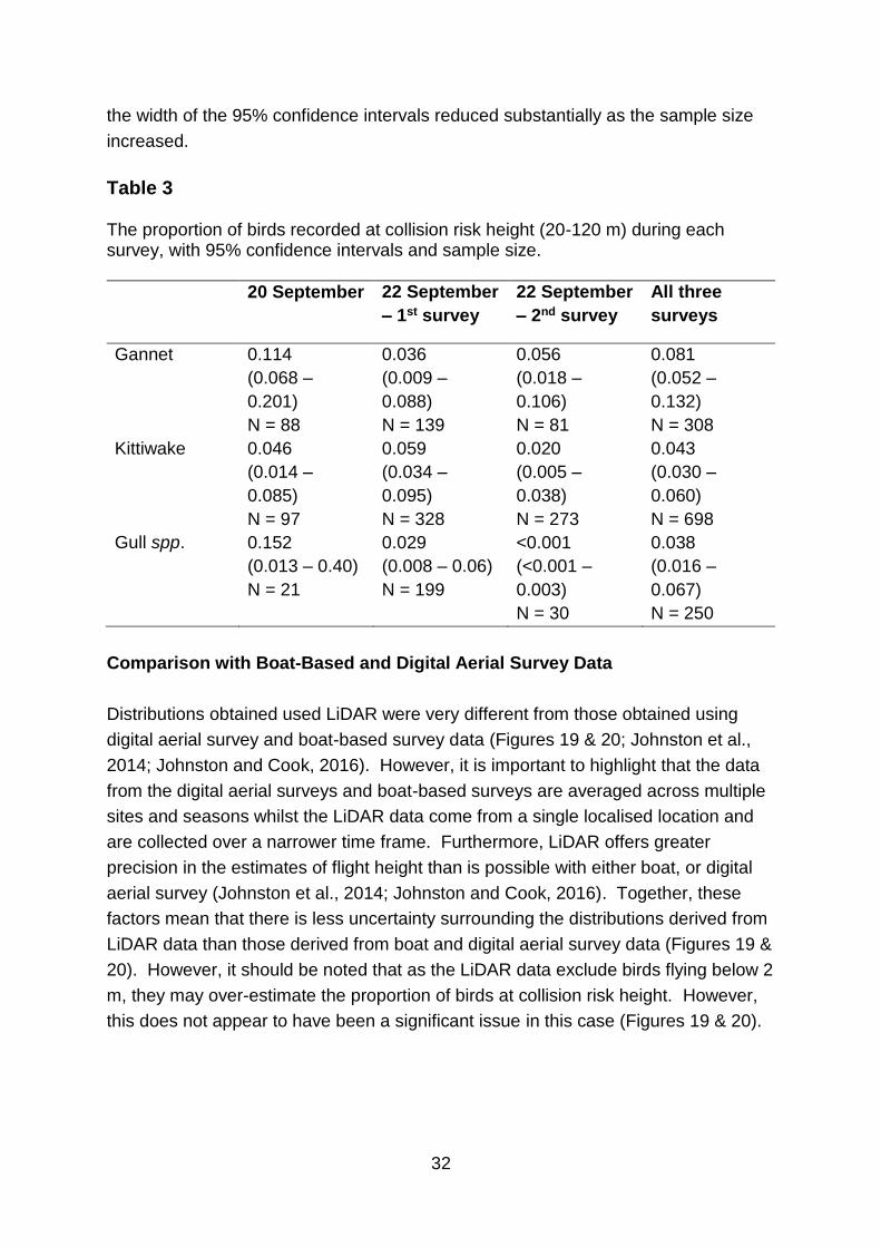
32
the width of the 95% confidence intervals reduced substantially as the sample size
increased.
Table 3 The proportion of birds recorded at collision risk height (20-120 m) during each survey, with 95% confidence intervals and sample size.
20 September 22 September
– 1st survey
22 September
– 2nd survey
All three
surveys
Gannet 0.114
(0.068 –
0.201)
N = 88
0.036
(0.009 –
0.088)
N = 139
0.056
(0.018 –
0.106)
N = 81
0.081
(0.052 –
0.132)
N = 308
Kittiwake 0.046
(0.014 –
0.085)
N = 97
0.059
(0.034 –
0.095)
N = 328
0.020
(0.005 –
0.038)
N = 273
0.043
(0.030 –
0.060)
N = 698
Gull spp. 0.152
(0.013 – 0.40)
N = 21
0.029
(0.008 – 0.06)
N = 199
<0.001
(<0.001 –
0.003)
N = 30
0.038
(0.016 –
0.067)
N = 250
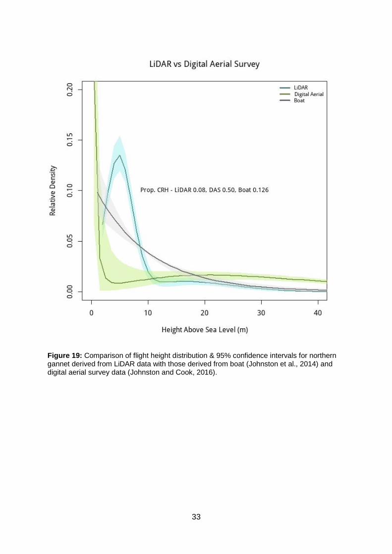
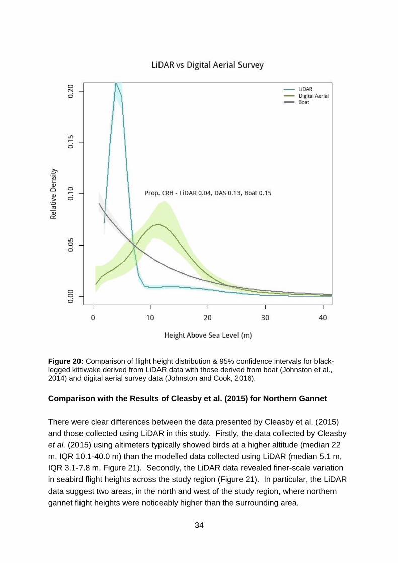
Comparison with Boat-Based and Digital Aerial Survey Data
Distributions obtained used LiDAR were very different from those obtained using
digital aerial survey and boat-based survey data (Figures 19 & 20; Johnston et al.,
2014; Johnston and Cook, 2016). However, it is important to highlight that the data
from the digital aerial surveys and boat-based surveys are averaged across multiple
sites and seasons whilst the LiDAR data come from a single localised location and
are collected over a narrower time frame. Furthermore, LiDAR offers greater
precision in the estimates of flight height than is possible with either boat, or digital
aerial survey (Johnston et al., 2014; Johnston and Cook, 2016). Together, these
factors mean that there is less uncertainty surrounding the distributions derived from
LiDAR data than those derived from boat and digital aerial survey data (Figures 19 &
20). However, it should be noted that as the LiDAR data exclude birds flying below 2
m, they may over-estimate the proportion of birds at collision risk height. However,
this does not appear to have been a significant issue in this case (Figures 19 & 20).
33
Figure 19: Comparison of flight height distribution & 95% confidence intervals for northern gannet derived from LiDAR data with those derived from boat (Johnston et al., 2014) and digital aerial survey data (Johnston and Cook, 2016).
34
Figure 20: Comparison of flight height distribution & 95% confidence intervals for black-legged kittiwake derived from LiDAR data with those derived from boat (Johnston et al., 2014) and digital aerial survey data (Johnston and Cook, 2016).
Comparison with the Results of Cleasby et al. (2015) for Northern Gannet
There were clear differences between the data presented by Cleasby et al. (2015)
and those collected using LiDAR in this study. Firstly, the data collected by Cleasby
et al. (2015) using altimeters typically showed birds at a higher altitude (median 22
m, IQR 10.1-40.0 m) than the modelled data collected using LiDAR (median 5.1 m,
IQR 3.1-7.8 m, Figure 21). Secondly, the LiDAR data revealed finer-scale variation
in seabird flight heights across the study region (Figure 21). In particular, the LiDAR
data suggest two areas, in the north and west of the study region, where northern
gannet flight heights were noticeably higher than the surrounding area.
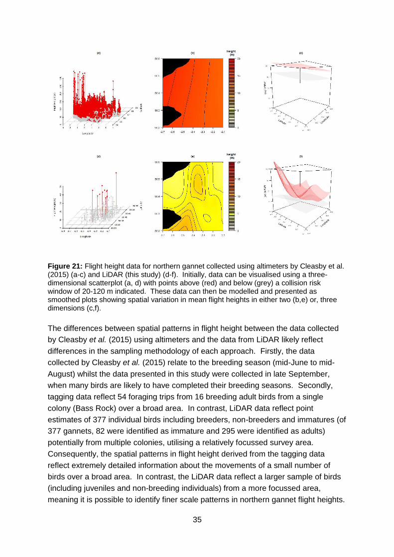
35
Figure 21: Flight height data for northern gannet collected using altimeters by Cleasby et al. (2015) (a-c) and LiDAR (this study) (d-f). Initially, data can be visualised using a three-dimensional scatterplot (a, d) with points above (red) and below (grey) a collision risk window of 20-120 m indicated. These data can then be modelled and presented as smoothed plots showing spatial variation in mean flight heights in either two (b,e) or, three dimensions (c,f).
The differences between spatial patterns in flight height between the data collected
by Cleasby et al. (2015) using altimeters and the data from LiDAR likely reflect
differences in the sampling methodology of each approach. Firstly, the data
collected by Cleasby et al. (2015) relate to the breeding season (mid-June to mid-
August) whilst the data presented in this study were collected in late September,
when many birds are likely to have completed their breeding seasons. Secondly,
tagging data reflect 54 foraging trips from 16 breeding adult birds from a single
colony (Bass Rock) over a broad area. In contrast, LiDAR data reflect point
estimates of 377 individual birds including breeders, non-breeders and immatures (of
377 gannets, 82 were identified as immature and 295 were identified as adults)
potentially from multiple colonies, utilising a relatively focussed survey area.
Consequently, the spatial patterns in flight height derived from the tagging data
reflect extremely detailed information about the movements of a small number of
birds over a broad area. In contrast, the LiDAR data reflect a larger sample of birds
(including juveniles and non-breeding individuals) from a more focussed area,
meaning it is possible to identify finer scale patterns in northern gannet flight heights.
36
However, it should be noted that, because of the more restricted area over which
these LiDAR data have been collected, these distributions are less likely to reflect
the full range of northern gannet flight behaviour (e.g. both foraging and commuting
flight).
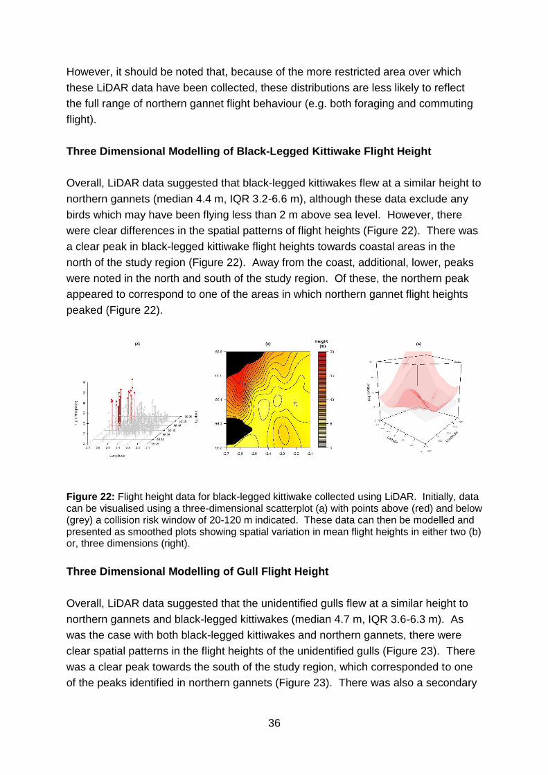
Three Dimensional Modelling of Black-Legged Kittiwake Flight Height
Overall, LiDAR data suggested that black-legged kittiwakes flew at a similar height to
northern gannets (median 4.4 m, IQR 3.2-6.6 m), although these data exclude any
birds which may have been flying less than 2 m above sea level. However, there
were clear differences in the spatial patterns of flight heights (Figure 22). There was
a clear peak in black-legged kittiwake flight heights towards coastal areas in the
north of the study region (Figure 22). Away from the coast, additional, lower, peaks
were noted in the north and south of the study region. Of these, the northern peak
appeared to correspond to one of the areas in which northern gannet flight heights
peaked (Figure 22).
Figure 22: Flight height data for black-legged kittiwake collected using LiDAR. Initially, data can be visualised using a three-dimensional scatterplot (a) with points above (red) and below (grey) a collision risk window of 20-120 m indicated. These data can then be modelled and presented as smoothed plots showing spatial variation in mean flight heights in either two (b) or, three dimensions (right).
Three Dimensional Modelling of Gull Flight Height
Overall, LiDAR data suggested that the unidentified gulls flew at a similar height to
northern gannets and black-legged kittiwakes (median 4.7 m, IQR 3.6-6.3 m). As
was the case with both black-legged kittiwakes and northern gannets, there were
clear spatial patterns in the flight heights of the unidentified gulls (Figure 23). There
was a clear peak towards the south of the study region, which corresponded to one
of the peaks identified in northern gannets (Figure 23). There was also a secondary
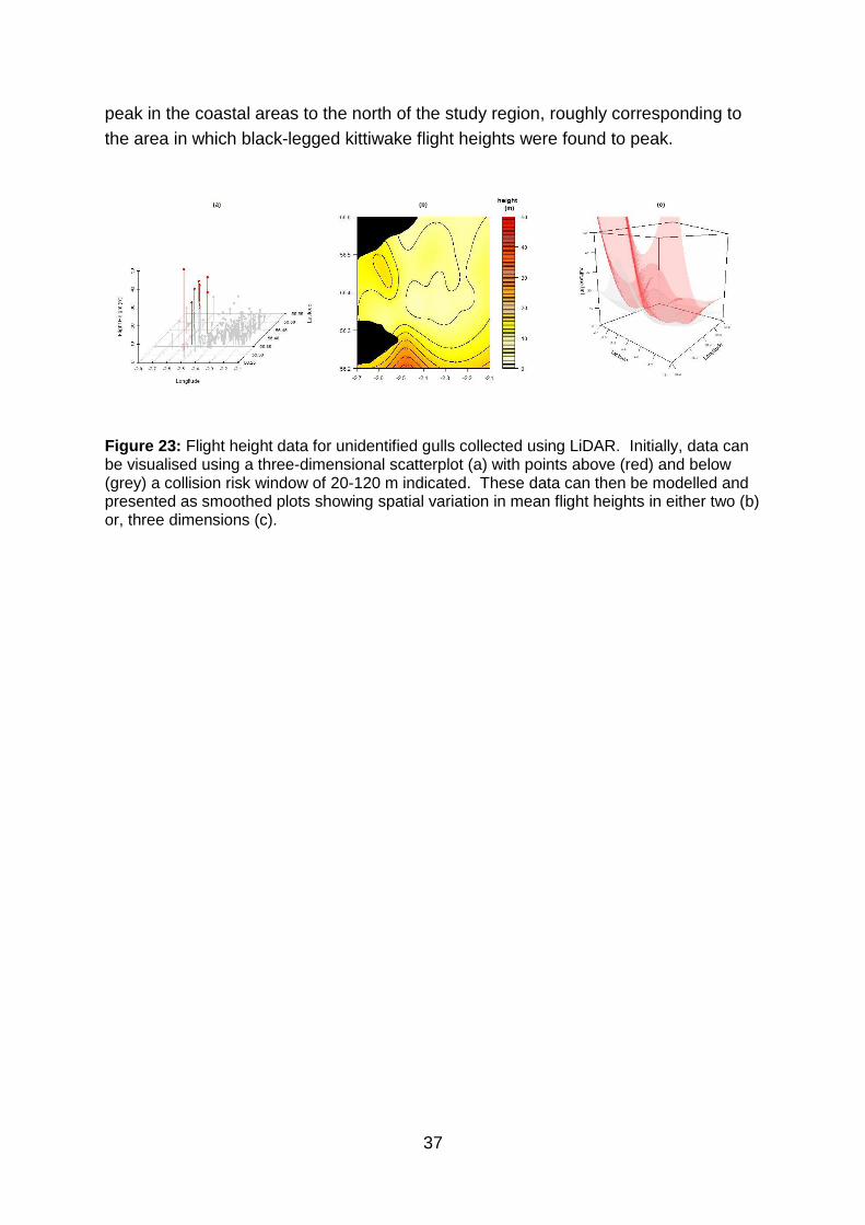
37
peak in the coastal areas to the north of the study region, roughly corresponding to
the area in which black-legged kittiwake flight heights were found to peak.
Figure 23: Flight height data for unidentified gulls collected using LiDAR. Initially, data can be visualised using a three-dimensional scatterplot (a) with points above (red) and below (grey) a collision risk window of 20-120 m indicated. These data can then be modelled and presented as smoothed plots showing spatial variation in mean flight heights in either two (b) or, three dimensions (c).
38
Discussion
Of the six objectives set at the start of the project, we have fulfilled four and partially
fulfilled the remaining two. We have successfully tested the novel combination of
LiDAR and digital imagery as a tool for collecting information about the flight heights
of seabirds. We have carried out a successful validation exercise which
demonstrates that this approach can measure seabird flight heights with a high
degree of precision. We have compared the flight heights measured using this
approach to those collected using boat-based surveys, digital aerial surveys and
GPS tags. We have demonstrated how this approach can be used to decrease
uncertainty in collision risk assessments through the use of spatial modelling of
species flight heights. However, we were only able to collect sufficient data to
produce modelled flight height distributions for two of the five key breeding seabird
features of UK SPAs. This reflects technical problems which meant that the
fieldwork had to be delayed until September, when most of the study species had
completed their breeding seasons.
Our analyses demonstrate that LiDAR can offer a valuable tool with which to
estimate seabird flight heights. In contrast to other approaches, LiDAR is capable of
measuring seabird flight heights with a high degree of precision, typically within 1 m
(Table 2). In comparison, the error associated with bird-borne devices can be more
variable. For GPS tags, error varies from approximately 3 m to 14 m depending on
factors such as the sampling rate that is used (Borkenhagen et al., 2018; Thaxter et
al., 2018) with a similar level of error for estimates derived from altimeters (Thaxter
et al., 2016). The error associated with “high end” laser rangefinders has been
estimated at approximately 2 m (Borkenhagen et al., 2018) whilst the estimates from
digital aerial survey are wider and more variable (Johnston and Cook, 2016).
Consequently, the uncertainty associated with measurements of seabird flight height
from LiDAR is far lower than the uncertainty associated with measurements made
using other technologies. Furthermore, flight heights are estimated relative to the
sea surface, helping to overcome difficulties associated with negative flight heights
that may be recorded when using digital aerial surveys, GPS tags or laser
rangefinders (Borkenhagen et al., 2018; Corman and Garthe, 2014; Johnston and
Cook, 2016; Ross-Smith et al., 2016).
A key limitation of LiDAR estimates of seabird flight height is that sea-swell may
interfere with the detection of birds in flight, resulting in a high false positive rate. For
the purposes of this study, flight height has been estimated with reference to height
above the mean sea level generated from each LiDAR pulse. As part of this study, a
lower threshold of 1-2 m above sea level, depending on when the survey was carried
39
out, was identified as a point at which the false positive rate was not unacceptably
high. As a consequence, the flight height distributions derived as part of this study
will be biased against birds flying below 1-2 m above sea level i.e. would
overestimate the proportion on birds at greater altitudes. However, this compares
favourably to the use of handheld laser rangefinders on a vessel which may be
biased against birds flying less than 10 m above sea level (Borkenhagen et al.,
2018). Furthermore, there is the potential to lower the threshold used in the analysis
of LiDAR data through further analytical development. By using an estimate of mean
sea-level, we are treating the water surface as a smooth plane. By using a
topographic model (e.g. Hwang et al., 2000) it would be possible to treat the water as
a ‘rough’ surface, more reflective of any sea-swell, and identify birds closer to the
sea-surface. However, it should be noted that such an approach may result in a
greater uncertainty surrounding estimated seabird flight heights as these estimates
would vary depending on whether a bird was detected over a wave or a trough.
To understand the potential consequences of the bias against low-flying birds
present in the data, we re-calculated the proportion of birds at collision risk height
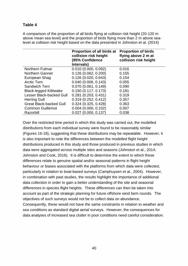
presented in Johnston et al. (2014) having excluded those flying below 2 m. For all
species, excluding birds flying below 2 m resulted in a modest increase in the
proportion of birds estimated to be at collision risk height (Table 4). However, the
proportional change in the number of birds flying at collision risk height was greatest
for species whose flight heights meant that they were generally at low risk of
collision. Furthermore, even after excluding birds flying below 2 m from the analysis,
the revised proportion of birds at collision risk height was well within the 95%
confidence intervals of that calculated from the full distribution (Table 4). As the
LiDAR in this study was unable to detect birds flying below 2 m, this is likely to result
in the distributions presented above over-estimating the proportion of birds at
collision risk height. Such an overestimate is likely to lead to a precautionary
assessment of collision risk. However, given the overall uncertainty that may be
associated with estimates of collision risk and flight height behaviour, this
overestimate is unlikely to be overly precautionary. In future analyses it may be
possible to use standard digital aerial survey processing methods to count birds
flying below the threshold and incorporate these into the distributions by assuming a
default value (e.g. 1 m).
40
Table 4 A comparison of the proportion of all birds flying at collision risk height (20-120 m above mean sea level) and the proportion of birds flying more than 2 m above sea-level at collision risk height based on the data presented in Johnston et al. (2014)
Proportion of all birds at collision risk height (95% Confidence Intervals)
Proportion of birds flying above 2 m at collision risk height
Northern Fulmar 0.010 (0.000, 0.092) 0.016 Northern Gannet 0.126 (0.062, 0.200) 0.155 European Shag 0.126 (0.020, 0.643) 0.154 Arctic Tern 0.040 (0.006, 0.143) 0.055 Sandwich Tern 0.070 (0.061, 0.149) 0.090 Black-legged Kittiwake 0.150 (0.117, 0.173) 0.181 Lesser Black-backed Gull 0.281 (0.203, 0.431) 0.319 Herring Gull 0.319 (0.252, 0.412) 0.357 Great Black-backed Gull 0.324 (0.325, 0.428) 0.363 Common Guillemot 0.004 (0.000, 0.102) 0.007 Razorbill 0.027 (0.000, 0.137) 0.038
Over the restricted time period in which this study was carried out, the modelled
distributions from each individual survey were found to be reasonably similar
(Figures 16-18), suggesting that these distributions may be repeatable. However, it
is also important to note the differences between the modelled flight height
distributions produced in this study and those produced in previous studies in which
data were aggregated across multiple sites and seasons (Johnston et al., 2014;
Johnston and Cook, 2016). It is difficult to determine the extent to which these
differences relate to genuine spatial and/or seasonal patterns in flight height
behaviour or biases associated with the platforms from which data were collected,
particularly in relation to boat-based surveys (Camphuysen et al., 2004). However,
in combination with past studies, the results highlight the importance of additional
data collection in order to gain a better understanding of the site and seasonal
differences in species flight heights. These differences can then be taken into
account as part of the strategic planning for future offshore wind farm rounds. The
objectives of such surveys would not be to collect data on abundance.
Consequently, these would not have the same constraints in relation to weather and
sea conditions as standard digital aerial surveys. However, the consequences for
data analyses of increased sea clutter in poor conditions need careful consideration.
41
Future Applications
Species flight heights are known to vary spatially and temporally (Cleasby et al.,
2015; Corman and Garthe, 2014; Ross-Smith et al., 2016). This variation may be
influenced by behaviour, for example whether birds are actively foraging or,
commuting between breeding colonies and preferred foraging areas (Cleasby et al.,
2015). In order to fully understand the extent of this variation and what influences it,
more data are required from a wider range of sites, seasons and conditions. In order
to understand how the presence of a wind farm may influence species flight
behaviour, this should include a survey area which incorporates a wind farm and a
substantial buffer area. Similar surveys have been carried out in order to assess the
distribution of northern gannets in relation to an offshore wind farm (APEM Ltd.,
2014). These surveys suggest that it may be challenging to collect sufficient data to
enable producing a modelled flight height distribution for northern gannet within a
wind farm. However, given that black-legged kittiwake and large gulls show little
displacement by, and may even be attracted to, offshore wind farms, it should be
possible to gain a sufficient sample size for these species (Dierschke et al., 2016;
Vanermen et al., 2015).
As with traditional digital aerial surveys, a key limitation in flight height estimates
using the approach described in this study is the difficulty in collecting data at night.
We know from GPS tracking studies that flight height may differ between day and
night (Ross-Smith et al., 2016). As with traditional digital aerial surveys, the key
limiting factor in using LiDAR to estimate the flight height of birds at night is the need
for digital imagery to accompany the LiDAR data in order to confirm the presence of
a bird and identify the species concerned. However, there may be the potential to
combine LiDAR with thermal imaging technology in order to detect birds at night (e.g.
Kinzel et al., 2006). Thermal imaging techniques have previously been used to
detect birds moving in and around offshore wind farms (Desholm et al., 2006). At
present, such technology may be insufficient to precisely identify the species
concerned, but it may be possible to assign birds to rough species groups (e.g. large
gulls, gannet, etc.).
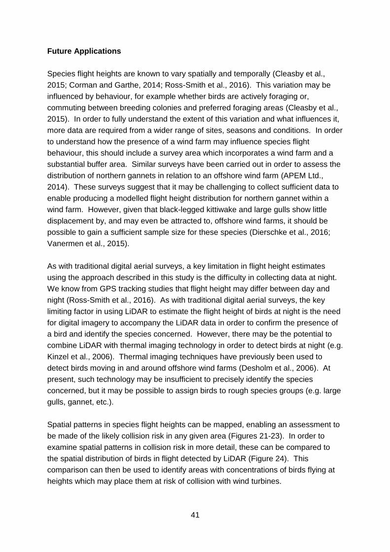
Spatial patterns in species flight heights can be mapped, enabling an assessment to
be made of the likely collision risk in any given area (Figures 21-23). In order to
examine spatial patterns in collision risk in more detail, these can be compared to
the spatial distribution of birds in flight detected by LiDAR (Figure 24). This
comparison can then be used to identify areas with concentrations of birds flying at
heights which may place them at risk of collision with wind turbines.
42
Figure 24: LiDAR data can be used to produce kernel density estimates of the distribution of birds in flight and show patterns of spatial variation in species flight heights. The kernel density estimates of species distributions can then be overlaid on to plots showing spatial patterns in species flight heights, enabling the two to be compared.
The models of the distribution of seabirds in flight and the heights at which they fly
presented in this report (Figure 24) are relatively simple analyses based on spatial
smoothing. However, there is the potential to improve these models through the
incorporation of environmental variables, for example in relation to oceanographic or
wind conditions (Ainley et al., 2015; Scott et al., 2013; Spear and Ainley, 2008). This
would enhance the predictive capability of these models, potentially enabling
assessments of collision risk to be extrapolated over a broader spatial area.
Irrespective of whether environmental variables are included, the models of the
distribution of seabirds in flight and the heights at which they fly presented in this
43
report provides an approach that is likely to be of value as a tool to the marine spatial
planning of the offshore wind sector.
The accuracy of estimates of bird flight speed can have a significant impact on
predictions about collision risk (Fijn and Gyimesi, 2018; Masden, 2015; Skov et al.,
2018). However, published estimates of flight speed are often based on a limited
sample of birds (e.g. Alerstam et al., 2007) and, as with flight height, it is clear that
there may be spatial patterns in flight speed related to birds behaviour (Fijn and
Gyimesi, 2018). A detailed assessment of species flight speeds has been
highlighted as a key gap in knowledge in relation to assessments of collision risk at
offshore wind farms (Masden, 2015). The approach to data collection used in this
study could enable the estimation of species flight speeds. The birds detected by
the LiDAR feature in two photographs, one immediately prior to the LiDAR pulse and
one immediately after the LiDAR pulse. These photographs can be georeferenced
and, because we have an accurate estimate of species flight height from the LiDAR,
the distance travelled by the bird between the two photographs can be estimated
using trigonometry. As we also know the time between each photograph, the flight
speed of the bird in question can then be estimated. Having done this, it would be
possible to either produce a modelled distribution of species flight speeds, as we
have done in relation to flight height or, to look at spatial variation in flight speed, as
in Figure 24. Combining plots of spatial patterns of species flight speed with those of
flight height and distribution would further improve spatial assessments of collision
risk, such as those which could be inferred from Figure 24. In additional to being of
value in relation to planning for the offshore wind sector, such assessments may be
of value for wider marine spatial planning purposes as they may enable an
assessment of spatial patterns in behaviour from which it may be possible to infer
how birds are using any given area (e.g. in relation to foraging, commuting or,
migration).
Best Practice Recommendations
LiDAR offers a valuable tool with which to estimate seabird flight heights. As the
methodology and approaches to data processing develop this technique may be a
valuable addition to traditional digital aerial surveys. Indeed, as methodologies
develop, LiDAR may help reduce the costs of traditional digital aerial surveys by
reducing the time needed for data processing if it can be used to filter images in
which birds are present on the sea surface.
44
Based on our experiences with this approach, we make the following
recommendations for future studies:
In order to balance the risk of disturbance to birds with the need for high
resolution imagery and high LiDAR point density, we recommend a minimum
survey aircraft altitude of 300 m above mean sea-level for survey aircraft. As
technology and analytical approaches improve, it is likely to be possible to
increase this altitude further.
In order to optimise the imagery, the flight speed of the survey aircraft and the
repetition rate of the camera should be optimised to ensure a minimum image
overlap of 60% in order to aid identification of birds detected by LiDAR. For
the purposes of this study, this reflected a ground speed of approximately 240
km h-1 and a camera repetition rate of 1.6 seconds.
To achieve a greater level of certainty in identification and a reduction in the
birds assigned to only species group level e.g. grey gulls, requires higher
photographic resolution than was used in this study. It is considered, based
on digital aerial surveys undertaken elsewhere, that a resolution of 2.5 cm
Ground Sampling Distance will be adequate in most instances.
The point density of the LiDAR should on survey be at least 10 points/m2 at
sea level to optimise on coverage in transect by the LiDAR.
Careful consideration should be given to ensuring that factors such as sea-
swell do not result in a high false positive rate when identifying birds in flight.
A high false positive rate may make it difficult to determine how LiDAR points
relate to birds in the accompanying photographs. Determining a threshold
below which the high false positive rate means data should be excluded from
the analysis is a key stage in data processing. This threshold may vary
depending on weather conditions.
The camera and LiDAR imagery originate from a single point. This means
that the three dimensional shape over which data are collected is a pyramid.
The consequence of this is that as the altitude of birds in flight increases, the
probability of them being detected decreases. Note that this is an issue for
flight heights measured using existing digital aerial survey protocols as well as
LiDAR. This difficulty can be overcome if the location of the bird is pinpointed
in three dimensions by recording both the duration and angle of the return
pulse from the LiDAR. By pinpointing the location of the bird in three
dimensions, difficulties in relation to detecting birds may be overcome either
through the application of statistical approaches such as occupancy
modelling, or by filtering based on distance from transect line, as in Figure 7.
45
In order to overcome this difficulty, the angle of the bird relative to the LiDAR
equipment should be recorded. This will allow the bird to be located in three
dimensions with a high degree of accuracy using basic trigonometry.
Assuming that birds are randomly distributed in relation to the transects and
the survey aircraft, when considered across the study region as a whole, the
distribution of the horizontal distances between the birds and the transect line
should be relatively even. This assumption should be confirmed and, if not
met, data beyond this region should be excluded from analysis.
Data represent a sample from the true distribution, rather than the distribution
itself. Consequently, simple plots of the proportion of birds recorded at
different heights will not reflect the true flight height distribution. Therefore, it
is important to use the data to produce a modelled distribution of seabird flight
heights. However, it is equally important that the distribution these data are
fitted to is sufficiently flexible to adapt to a range of different shapes. If the
distribution is relatively inflexible, the final flight height distribution may be
constrained to reflect the assumed distribution, rather than the flight heights of
the species in question. For this reason, a range of distributions should be
considered for modelling bird flight heights and, careful consideration should
be given as to which best matches the observed data.
Sample size is a key factor in determining how well a modelled distribution
can reflect the true underlying distribution. A minimum sample size of 100
birds from each site and/or seasons being considered offers an optimal
balance between being able to fit a robust flight height distribution and a
realistic level of effort for surveys.

46
Acknowledgements
This work was funded by the Contract Research Fund of the Scottish Government
and overseen by a project steering group consisting of Marine Scotland, Marine
Scotland Science, RSPB, Natural England, JNCC, Crown Estate and Scottish
Natural Heritage. Jim Kersey (NIRAS) and Penny Mitchell (BTO) also provided
valuable support for the project. Nick Brockie (SSE), Jesper Larsen (Vatenfall),
Sophie Hartfield and Rachel Hall (both Ørsted) proved useful insights from a
developer’s perspective. Thanks also to Peter Lund Hansen (FUGRO) for advice
about the LiDAR equipment, and Arjun Sheoran and Helica Srl. for supplying the
LiDAR equipment used for this work. James Hutton Institute offered us access to
land for our initial validation exercise, which Nicola Largey and Elizabeth Masden
(UHI ERI) also offered helpful advice and assistance with. Keith Hamer (University
of Leeds) and Ian Cleasby (University of Exeter) supplied northern gannet tracking
data from the study region. Matt Hazleton (NIRAS UK) helped with the initial
fieldwork planning and identification of the study site. Morten Fredskild (NIRAS)
helped with the processing of the data collected as part of the validation exercise.
Alison Johnston, Chris Thaxter and Niall Burton (BTO) offered valuable comments
and advice on this work. Thanks also to Marine Scotland and Airtask Group for their
assistance with the aircraft and deploying the equipment for the survey.
47
References
Ainley, D.G., Porzig, E., Zajanc, D., Spear, L.B., 2015. Seabird flight behavior and
height in response to altered wind strength and direction. Marine Ornithology 43, 25-
36.
Alerstam, T., Rosén, M., Bäckman, J., Ericson, P.G.P., Hellgren, O., 2007. Flight
Speeds among Bird Species: Allometric and Phylogenetic Effects. PLoS Biology 5,
e197. https://doi.org/10.1371/journal.pbio.0050197
APEM Ltd., 2014. Assessing northern gannet avoidance of offshore wind farms.
Cambridge.
Azmy, S.N., Sah, S.A.M., Shafie, N.J., Ariffin, A., Majid, Z., Ismail, M.N.A., Shamsir,
M.S., 2012. Counting in the dark: Non-intrusive laser scanning for population
counting and identifying roosting bats. Scientific Reports 2, 524.
https://doi.org/10.1038/srep00524
Band, B., 2012. Using a collision risk model to assess bird collision risks for offshore
wind farms [WWW Document]. URL
https://www.bto.org/sites/default/files/u28/downloads/Projects/Final_Report_SOSS02
_Band1ModelGuidancepdf (accessed 8.23.17)
Benaglia, T., Chauveau, D., Hunter, D.R., Young, D., 2009. mixtools : An R Package
for Analyzing Finite Mixture Models. Journal of Statistical Software 32, 1-29.
https://doi.org/10.18637/jss.v032.i06
Borkenhagen, K., Corman, A.-M., Garthe, S., 2018. Estimating flight heights of
seabirds using optical rangefinders and GPS data loggers: a methodological
comparison. Marine Biology 165, 17. https://doi.org/10.1007/s00227-017-3273-z
Camphuysen, C. J., Fox, A., Leopold, M., Petersen, I. K. 2004. Towards
Standardised Seabirds at Sea Census Techniques in Connection with Environmental
Impact Assessments for Offshore Wind Farms in the UK. Report by Royal
Netherlands Institute for Sea Research (NIOZ). pp 39.
Chust, G., Galparsoro, I., Borja, Á., Franco, J., Uriarte, A., 2008. Coastal and
estuarine habitat mapping, using LIDAR height and intensity and multi-spectral
imagery. Estuarine, Coastal and Shelf Science 78, 633-643.
https://doi.org/10.1016/J.ECSS.2008.02.003
48
Cleasby, I.R., Wakefield, E.D., Bearhop, S., Bodey, T.W., Votier, S.C., Hamer, K.C.,
2015. Three-dimensional tracking of a wide-ranging marine predator: Flight heights
and vulnerability to offshore wind farms. Journal of Applied Ecology 52, 1474-1482.
https://doi.org/10.1111/1365-2664.12529
Corman, A.M., Garthe, S., 2014. What flight heights tell us about foraging and
potential conflicts with wind farms: a case study in Lesser Black-backed Gulls (Larus
fuscus). Journal of Ornithology 155, 1037-1043. https://doi.org/10.1007/s10336-014-
1094-0
Delignette-Muller, M.L., Dutang, C., 2015. fitdistrplus: An R Package for Fitting
Distributions. Journal of Statistical Software 64, 1-34.
Desholm, M., Fox, A.D., Beasley, P.D.L., Kahlert, J., 2006. Remote techniques for
counting and estimating the number of bird-wind turbine collisions at sea: A review.
Ibis 148, 76-89. https://doi.org/10.1111/j.1474-919X.2006.00509.x
Dierschke, V., Furness, R.W., Garthe, S., 2016. Seabirds and offshore wind farms in
European waters: Avoidance and attraction. Biological Conservation 202, 59-68.
https://doi.org/10.1016/J.BIOCON.2016.08.016
Fijn, R.C., Gyimesi, A., 2018. Behaviour related flight speeds of Sandwich Terns
and their implications for wind farm collision rate modelling and impact assessment.
Environmental Impact Assessment Review 71, 12-16.
https://doi.org/10.1016/J.EIAR.2018.03.007
Fristrup, K.M., Shaw, J.A., Tauc, M.J., 2017. Development of a wing-beat-
modulation scanning lidar system for insect studies, in: Singh, U.N. (Ed.), Lidar
Remote Sensing for Environmental Monitoring 2017. SPIE, p. 15.
https://doi.org/10.1117/12.2274656
Furness, R.W., Wade, H.M., Masden, E.A., 2013. Assessing vulnerability of marine
bird populations to offshore wind farms. Journal of Environmental Management 119,
56-66. https://doi.org/10.1016/j.jenvman.2013.01.025
Garthe, S., Huppop, O., 2004. Scaling possible adverse effects of marine wind
farms on seabirds: Developing and applying a vulnerability index. Journal of Applied
Ecology 41, 724-734. https://doi.org/10.1111/j.0021-8901.2004.00918.x
49
HiDef, 2016. Kernel density analysis of seabird abundance and distribution in the
Outer Firth of Tay. Report to Marine Scotland.
Hill, R.A., Thomson, A.G., 2005. Mapping woodland species composition and
structure using airborne spectral and LiDAR data. International Journal of Remote
Sensing 26, 3763-3779. https://doi.org/10.1080/01431160500114706
Hwang, P.A., Wang, D.W., Walsh, E.J., Krabill, W.B., Swift, R.N., Hwang, P.A.,
Wang, D.W., Walsh, E.J., Krabill, W.B., Swift, R.N., 2000. Airborne Measurements
of the Wavenumber Spectra of Ocean Surface Waves. Part I: Spectral Slope and
Dimensionless Spectral Coefficient*. Journal of Physical Oceanography 30, 2753-
2767. https://doi.org/10.1175/1520-0485(2001)031<2753:AMOTWS>2.0.CO;2
Jansson, S., Brydegaard, M., Papayannis, A., Tsaknakis, G., Åkesson, S., 2017.
Exploitation of an atmospheric lidar network node in single-shot mode for the
classification of aerofauna. Journal of Applied Remote Sensing 11.
https://doi.org/10.1117/1.JRS.11.036009
Jansson, S., Papayannis, A., Åkesson, S., Tsaknakis, G., Brydegaard, M., 2016.
Exploitation of Multi-Band Lidar for the Classification of Free-Flying Migratory Birds:
A Pilot Study Over Athens, Greece. EPJ Web of Conferences 119, 27002.
https://doi.org/10.1051/epjconf/201611927002
Johnston, A., Cook, A.S.C.P., 2016. How high do birds fly? Development of
methods and analysis of digital aerial data of seabird flight heights. BTO Research
Report No. 676. Thetford.
Johnston, A., Cook, A.S.C.P., Wright, L.J., Humphreys, E.M., Burton, N.H.K., 2014.
Modelling flight heights of marine birds to more accurately assess collision risk with
offshore wind turbines. Journal of Applied Ecology 51, 31-41.
https://doi.org/10.1111/1365-2664.12191
Kinzel, P.J., Nelson, J.M., Paker, R.S., Davis, L.R., 2006. Spring Census of Mid‐
Continent Sandhill Cranes Using Aerial Infrared Videography. The Journal of
Wildlife Management 70, 70-77. https://doi.org/10.2193/0022-
541X(2006)70[70:SCOMSC]2.0.CO;2
Kirkeby, C., Wellenreuther, M., Brydegaard, M., 2016. Observations of movement
dynamics of flying insects using high resolution lidar. Scientific Reports 6, 29083.
https://doi.org/10.1038/srep29083
50
Kohlbrenner, D.A., Specialist, G., Jamison, T.A., Kedzierski, L.M., 2009. Automated
extraction of vertical obstructions from LiDAR data, in: ASPRS/MAPPS 2009 Fall
Conference. San Antonio, Texas.
Lefsky, M.A., Cohen, W.B., Parker, G.G., Harding, D.J., 2002. Lidar Remote
Sensing for Ecosystem Studies. BioScience 52, 19-30. https://doi.org/10.1641/0006-
3568(2002)052[0019:lrsfes]2.0.co;2
Martner, B.E., Moran, K.P., 2001. Using cloud radar polarization measurements to
evaluate stratus cloud and insect echoes. Journal of Geophysical Research:
Atmospheres 106, 4891-4897. https://doi.org/10.1029/2000JD900623
Masden, E. 2015. Developing an avian collision risk model to incorporate variability
and uncertainty. Scottish Marine and Freshwater Science Vol 6 No 14. Edinburgh:
Scottish Government, 43pp. DOI: 10.7489/1659-1
Northend, C.A., Honey, R.C., Evans, W.E., 1966. Laser Radar (Lidar) for
Meteorological Observations. Review of Scientific Instruments 37, 393-400.
https://doi.org/10.1063/1.1720199
R Core Team, 2014. R: A language and environment for statistical computing. R
Foundation for Statistical Computing, Vienna, Austria.
Ross-Smith, V.H., Thaxter, C.B., Masden, E.A., Shamoun-Baranes, J., Burton,
N.H.K., Wright, L.J., Rehfisch, M.M., Johnston, A., 2016. Modelling flight heights of
lesser black-backed gulls and great skuas from GPS: a Bayesian approach. Journal
of Applied Ecology 53, 1676-1685. https://doi.org/10.1111/1365-2664.12760
Scott, B.E., Webb, A., Palmer, M.R., Embling, C.B., Sharples, J., 2013. Fine scale
bio-physical oceanographic characteristics predict the foraging occurrence of
contrasting seabird species; Gannet (Morus bassanus) and storm petrel (Hydrobates
pelagicus). Progress in Oceanography 117, 118-129.
https://doi.org/10.1016/J.POCEAN.2013.06.011
Skov, H., Heinanen, S., Norman, T., Ward, R., Mendez-Roldan, S., Ellis, I., 2018.
ORJIP Bird Collision and Avoidance Study. Final report - April 2018.
https://www.carbontrust.com/resources/reports/technology/bird-collision-avoidance/
Spear, L.B., Ainley, D.G., 2008. Flight speed of seabirds in relation to wind speed
and direction. Ibis 139, 234-251. https://doi.org/10.1111/j.1474-919X.1997.tb04621.x
51
Stone, C.J., Webb, A., Barton, C., Ratcliffe, N., Reed, T.C., Tasker, M.L.,
Camphuysen, C.J., Pienkowski, M.W., 1995. An atlas of seabird distribution in
north-west European waters, pp. 326, ISBN 1 873701 94 2. Available from:
http://jncc.defra.gov.uk/page-2407
Thaxter, C.B., Burton, N.H.K., 2009. High Definition Imagery for Surveying Seabirds
and Marine Mammals: A Review of Recent Trials and Development of Protocols.
BTO Report to COWRIE. Thetford.
Thaxter, C.B., Ross-Smith, V.H., Bouten, W., Masden, E.A., Clark, N.A., Conway,
G.J., Barber, L., Clewley, G., Burton, N.H.K., 2018. Dodging the blades: new
insights into three-dimensional area use of offshore wind farms by lesser black-
backed gulls Larus fuscus. Marine Ecology Progress Series 587, 247-253.
https://doi.org/10.3354/meps12415
Thaxter, C.B., Ross-Smith, V.H., Cook, A.S.C.P., 2016. How high do birds fly? A
review of current datasets and an appraisal of current methodologies for collecting
flight height data: Literature Review. BTO Research Report No. 666. Thetford.
Vanermen, N., Onkelinx, T., Courtens, W., Van de walle, M., Verstraete, H., Stienen,
E.W.M., 2015. Seabird avoidance and attraction at an offshore wind farm in the
Belgian part of the North Sea. Hydrobiologia 756, 51-61.
https://doi.org/10.1007/s10750-014-2088-x
Vierling, K.T., Vierling, L.A., Gould, W.A., Martinuzzi, S., Clawges, R.M., 2008.
Lidar: shedding new light on habitat characterization and modelling. Frontiers in
Ecology and the Environment 6, 90-98. https://doi.org/10.1890/070001
Wood, S.N., 2006. Generalised Additive Models: An Introduction With R. CRC
Press, Boca Raton, Florida.
52
APPENDIX 1
Validation Exercise
Aims
The purpose of the validation test is to demonstrate the efficacy and accuracy of a
LiDAR capture approach by comparing estimated seabird flight heights using
airborne LiDAR to objects of known height. Drones are flown at known heights and
varying speeds.
Initial (Unsuccessful) Data Validation Exercise
The initial data validation exercise was planned for Balruddery Farm, Invergowrie,
Dundee (56.48˚N, 3.13˚W), with the kind permission of the landowners, the James
Hutton Institute. The site was selected on the requirement for a comparatively level
open area free from obstructions e.g. pylons at no closer than 200 metres, within
which UK regulations permit the flying of drones and the low level flying of aircraft
down to approximately 300 m. The site chosen covered two lowland arable fields
within proximity to the Tay estuary. Unfortunately, weather conditions meant that
this had to be aborted.
To carry out the data validation exercise, it was intended for the survey aircraft to fly
over the study site for approximately one hour in order to capture the drone with the
LiDAR equipment. The flight path for the aircraft when crossing the two fields at the
site was to start at 56.48˚N, 3.13˚W and end at 56.48˚N, 3.14˚W. This was
considered by the aircraft operators (Airtask) to be safe and achievable.
The drone to be used for the survey was a Mikrokopter OKTO XL equipped with a
GPS, barometric altitude meter and accelerometer. This drone has a maximum
diameter of 1 m and a height of 0.38 m. The Mikrokopter can operate in wind
conditions of up to gusts of 12 m/s and a temperature range of -15-+35 degrees
Celsius. The drone was piloted by a CAA approved pilot (Simon Strickland, Dragons
Eye Filming [CAA licence no. PA and EUAV1931]). To comply with CAA licence
requirements, the pilot maintained direct visual contact with the drone at all times
and the drone was to be flown below a ceiling height of 120 metres.
The drone was to be flown at known heights and varying speeds, so as to intersect
under the flight path of the survey aircraft flying at 1,000 feet (305 metres) and no
lower than 250 metres (820 feet).
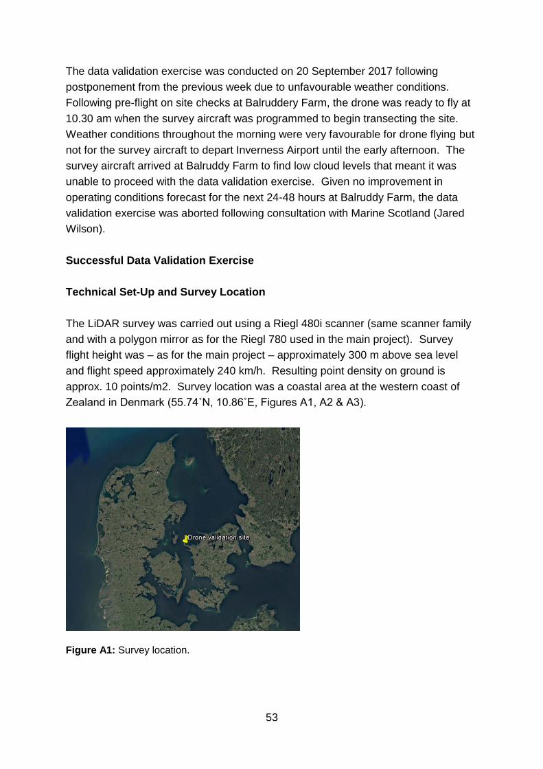
53
The data validation exercise was conducted on 20 September 2017 following
postponement from the previous week due to unfavourable weather conditions.
Following pre-flight on site checks at Balruddery Farm, the drone was ready to fly at
10.30 am when the survey aircraft was programmed to begin transecting the site.
Weather conditions throughout the morning were very favourable for drone flying but
not for the survey aircraft to depart Inverness Airport until the early afternoon. The
survey aircraft arrived at Balruddy Farm to find low cloud levels that meant it was
unable to proceed with the data validation exercise. Given no improvement in
operating conditions forecast for the next 24-48 hours at Balruddy Farm, the data
validation exercise was aborted following consultation with Marine Scotland (Jared
Wilson).
Successful Data Validation Exercise
Technical Set-Up and Survey Location
The LiDAR survey was carried out using a Riegl 480i scanner (same scanner family
and with a polygon mirror as for the Riegl 780 used in the main project). Survey
flight height was – as for the main project – approximately 300 m above sea level
and flight speed approximately 240 km/h. Resulting point density on ground is
approx. 10 points/m2. Survey location was a coastal area at the western coast of
Zealand in Denmark (55.74˚N, 10.86˚E, Figures A1, A2 & A3).
Figure A1: Survey location.
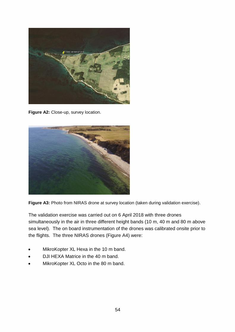
54
Figure A2: Close-up, survey location.
Figure A3: Photo from NIRAS drone at survey location (taken during validation exercise).
The validation exercise was carried out on 6 April 2018 with three drones
simultaneously in the air in three different height bands (10 m, 40 m and 80 m above
sea level). The on board instrumentation of the drones was calibrated onsite prior to
the flights. The three NIRAS drones (Figure A4) were:
MikroKopter XL Hexa in the 10 m band.
DJI HEXA Matrice in the 40 m band.
MikroKopter XL Octo in the 80 m band.
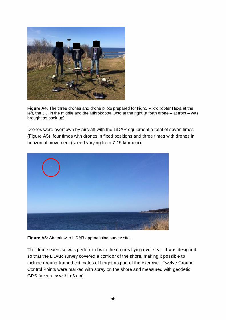
55
Figure A4: The three drones and drone pilots prepared for flight, MikroKopter Hexa at the left, the DJI in the middle and the Mikrokopter Octo at the right (a forth drone – at front – was brought as back-up).
Drones were overflown by aircraft with the LiDAR equipment a total of seven times
(Figure A5), four times with drones in fixed positions and three times with drones in
horizontal movement (speed varying from 7-15 km/hour).
Figure A5: Aircraft with LiDAR approaching survey site.
The drone exercise was performed with the drones flying over sea. It was designed
so that the LiDAR survey covered a corridor of the shore, making it possible to
include ground-truthed estimates of height as part of the exercise. Twelve Ground
Control Points were marked with spray on the shore and measured with geodetic
GPS (accuracy within 3 cm).
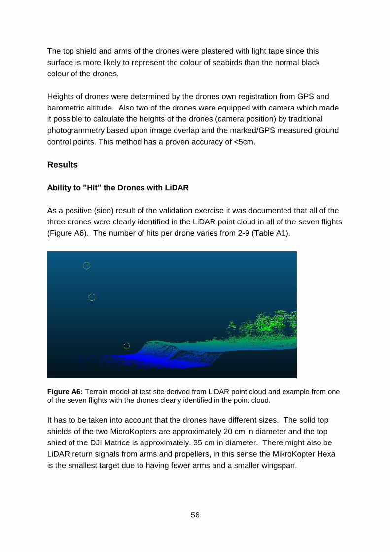
56
The top shield and arms of the drones were plastered with light tape since this
surface is more likely to represent the colour of seabirds than the normal black
colour of the drones.
Heights of drones were determined by the drones own registration from GPS and
barometric altitude. Also two of the drones were equipped with camera which made
it possible to calculate the heights of the drones (camera position) by traditional
photogrammetry based upon image overlap and the marked/GPS measured ground
control points. This method has a proven accuracy of <5cm.
Results
Ability to ”Hit” the Drones with LiDAR
As a positive (side) result of the validation exercise it was documented that all of the
three drones were clearly identified in the LiDAR point cloud in all of the seven flights
(Figure A6). The number of hits per drone varies from 2-9 (Table A1).
Figure A6: Terrain model at test site derived from LiDAR point cloud and example from one of the seven flights with the drones clearly identified in the point cloud.
It has to be taken into account that the drones have different sizes. The solid top
shields of the two MicroKopters are approximately 20 cm in diameter and the top
shied of the DJI Matrice is approximately. 35 cm in diameter. There might also be
LiDAR return signals from arms and propellers, in this sense the MikroKopter Hexa
is the smallest target due to having fewer arms and a smaller wingspan.
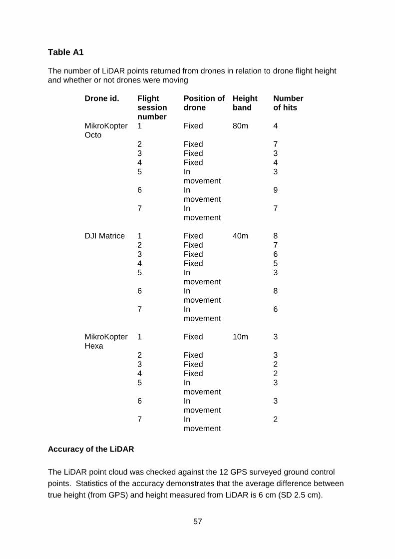
57
Table A1 The number of LiDAR points returned from drones in relation to drone flight height and whether or not drones were moving
Drone id. Flight session number
Position of drone
Height band
Number of hits
MikroKopter Octo
1 Fixed 80m 4
2 Fixed 7 3 Fixed 3 4 Fixed 4 5 In
movement 3
6 In movement
9
7 In movement
7
DJI Matrice 1 Fixed 40m 8 2 Fixed 7 3 Fixed 6 4 Fixed 5 5 In
movement 3
6 In movement
8
7 In movement
6
MikroKopter Hexa
1 Fixed 10m 3
2 Fixed 3 3 Fixed 2 4 Fixed 2 5 In
movement 3
6 In movement
3
7 In movement
2
Accuracy of the LiDAR
The LiDAR point cloud was checked against the 12 GPS surveyed ground control
points. Statistics of the accuracy demonstrates that the average difference between
true height (from GPS) and height measured from LiDAR is 6 cm (SD 2.5 cm).
58
It can be expected that the LiDAR measurements of the drones/birds has a similar
accuracy although difficult to prove since a bird (as well as a drone) is not in a fixed
position within this tolerance.
The test demonstrated that it was more complicated than expected to extract high
accuracy height information from the drones own GPS- and barometric altitude
registration since the registrations are not precisely related to the absolute reference
system and neither to the sea surface.
To compensate for this NIRAS used the camera exposures from two of the drones to
do a traditional photogrammetric height determination. Comparing the
photogrammetric height determination of the drones with the heights from the LiDAR
survey the difference is 33 cm in one test (DJI drone in 40 band) and 17 cm in
another test (MikroKopter Octo in 80 m band). These results are considered to be
“high accuracy” taking into account that it’s not possible to have an exact match of
the timestamps from the LiDAR acquisition and from the image exposures.
Based upon these experiences NIRAS conclude that the absolute height positioning
of the drones by LiDAR is actually better than the height information directly
registered by the drone.
The heights of the drones based upon LiDAR were compared with the heights
registered by the drone but with an off-set correction of the height information from
the drones to match the correct absolute height reference (Table A2). As for the DJI
drone it was not possible to extract the internal registration of height, so the
difference of 33 cm represents the result of the test comparing the photogrammetric
calculated height with the LiDAR height.
The differences are within 1 m (Table A2). Again one has to take into consideration
that it is not possible to have an exact match between the timestamps of the LiDAR
acquisition and the timestamps of the drone position meaning that the actual LiDAR
survey is expected to be better.
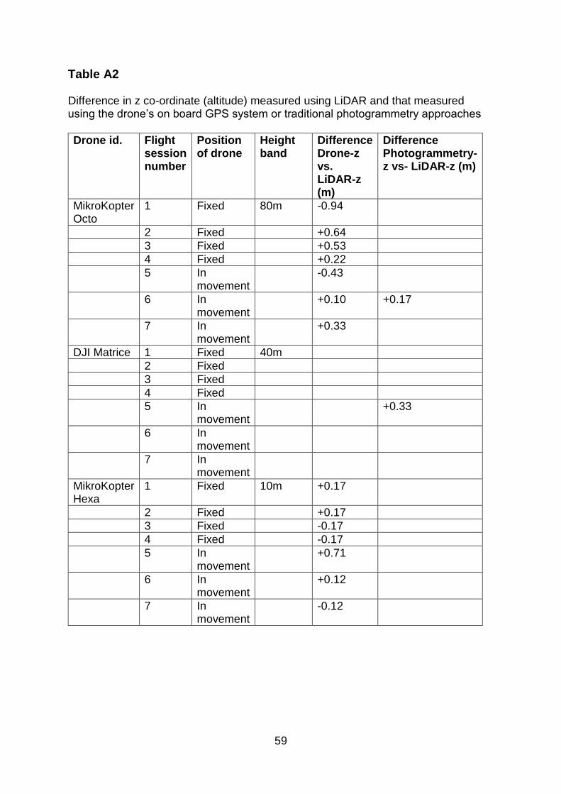
59
Table A2 Difference in z co-ordinate (altitude) measured using LiDAR and that measured using the drone’s on board GPS system or traditional photogrammetry approaches
Drone id. Flight session number
Position of drone
Height band
Difference Drone-z vs. LiDAR-z (m)
Difference Photogrammetry-z vs- LiDAR-z (m)
MikroKopter Octo
1 Fixed 80m -0.94
2 Fixed +0.64
3 Fixed +0.53
4 Fixed +0.22
5 In movement
-0.43
6 In movement
+0.10 +0.17
7 In movement
+0.33
DJI Matrice 1 Fixed 40m
2 Fixed
3 Fixed
4 Fixed
5 In movement
+0.33
6 In movement
7 In movement
MikroKopter Hexa
1 Fixed 10m +0.17
2 Fixed +0.17
3 Fixed -0.17
4 Fixed -0.17
5 In movement
+0.71
6 In movement
+0.12
7 In movement
-0.12