Hopper SOME EXTRACTS FROM THE BOOK BELT FEEDER … Feeder/Extract from the book... · Page 2...
93
Page 1 SOME EXTRACTS FROM THE BOOK – BELT FEEDER DESIGN AND HOPPER BIN SILO The information in this book extract is part of book and accordingly it is protected under copyright. However website visitor can copy this for his own use; not for publication or display. Chapter 1: FEEDER TYPES AND APPLICATION 1.1.0 NEED OF FEEDERS IN A SYSTEM The properly designed bulk material handling system always commences from the feeder, i.e. first equipment in the system (or section of the system), should always be feeder. This is depicted schematically in figure-1A. The feeder decides the magnitude of load on the system. Therefore, the system load condition and thereby its performance is governed / controlled by the feeder. For example, a belt conveyor conveys the material; whatever quantity is loaded onto it. If the quantity is loaded on the belt is less than its capability, then it will run at partial capacity. However, if the quantity loaded is excessive then the conveyor will be overloaded, spillage and even failure. The belt conveyor which has correct magnitude of load will have optimum performance, long life, maximum monetary return from investment. Similarly, if the receiving equipment happens to be crusher instead of conveyor, then, it will also have under- loading or correct-loading or overloading with consequential outcome (there can be few types of crushers which are suitable for choke-feed, but then that crusher will be also working as feeder-cum-crusher). As said before; any section of bulk material handling system always commences with feed control, i.e. mostly, by the equipment named as feeder. However, sometimes starting equipment may not be named as feeder, but it might actually be functioning indirectly as feeder also. For example, in a reclaiming system, the first equipment could be bucket wheel reclaimer. It is named as reclaimer, but in reality it is functioning as reclaimer and also as Feeder Material handling system Material input Figure-1A (schematic) Figure-1B (schematic) Hopper Feeder Conveyor Conveyor Screen Crusher Conveyor Conveyor
Transcript of Hopper SOME EXTRACTS FROM THE BOOK BELT FEEDER … Feeder/Extract from the book... · Page 2...

Page 1
SOME EXTRACTS FROM THE BOOK – BELT FEEDER DESIGN AND
HOPPER BIN SILO
The information in this book extract is part of book and accordingly it is protected under copyright.
However website visitor can copy this for his own use; not for publication or display.
Chapter 1: FEEDER TYPES AND APPLICATION
1.1.0 NEED OF FEEDERS IN A SYSTEM
The properly designed bulk material
handling system always
commences from the feeder, i.e.
first equipment in the system (or
section of the system), should
always be feeder. This is depicted
schematically in figure-1A. The feeder decides the magnitude of load on the system. Therefore, the system load
condition and thereby its performance is governed / controlled by the feeder.
For example, a belt conveyor conveys the material; whatever quantity is loaded onto it. If the quantity is loaded
on the belt is less than its capability, then it will run at partial capacity. However, if the quantity loaded is
excessive then the
conveyor will be
overloaded, spillage and
even failure. The belt
conveyor which has
correct magnitude of load
will have optimum
performance, long life,
maximum monetary return
from investment. Similarly,
if the receiving equipment
happens to be crusher
instead of conveyor, then,
it will also have under-
loading or correct-loading
or overloading with
consequential outcome (there can be few types of crushers which are suitable for choke-feed, but then that
crusher will be also working as feeder-cum-crusher).
As said before; any section of bulk material handling system always commences with feed control, i.e. mostly, by
the equipment named as feeder. However, sometimes starting equipment may not be named as feeder, but it
might actually be functioning indirectly as feeder also. For example, in a reclaiming system, the first equipment
could be bucket wheel reclaimer. It is named as reclaimer, but in reality it is functioning as reclaimer and also as
Feeder Material handling system
Material input
Figure-1A (schematic)
Figure-1B (schematic)
Hopper
Feeder
Conveyor
Conveyor
Screen
Crusher
Conveyor
Conveyor
Page 2
feeder, because it is accepting only specific maximum quantity of material from stock pile and then passing it to
down-line system.
The bulk material handling system (or section of the system) is made-up of handling equipment in series. In this
arrangement; the material from one equipment flows into second equipment, and from there to third equipment
and so on; as shown in figure-1B (refer page 1). So far these equipment in series are operating simultaneously
and at the same capacity, then there would not be feeder (for feed regulation) at intermediate point, as it would
introduce disturbance into stabilised flow pattern. Thus, feeder is not required among series of equipment, when
their operation is identical with respect to time and flow rate. In short, the first equipment in any section of bulk
material handling system needs to be feeder or equipment with feed control. The subsequent equipment in that
section does not need (have) feed regulation, unless its flow pattern is disturbed by items like storage facility.
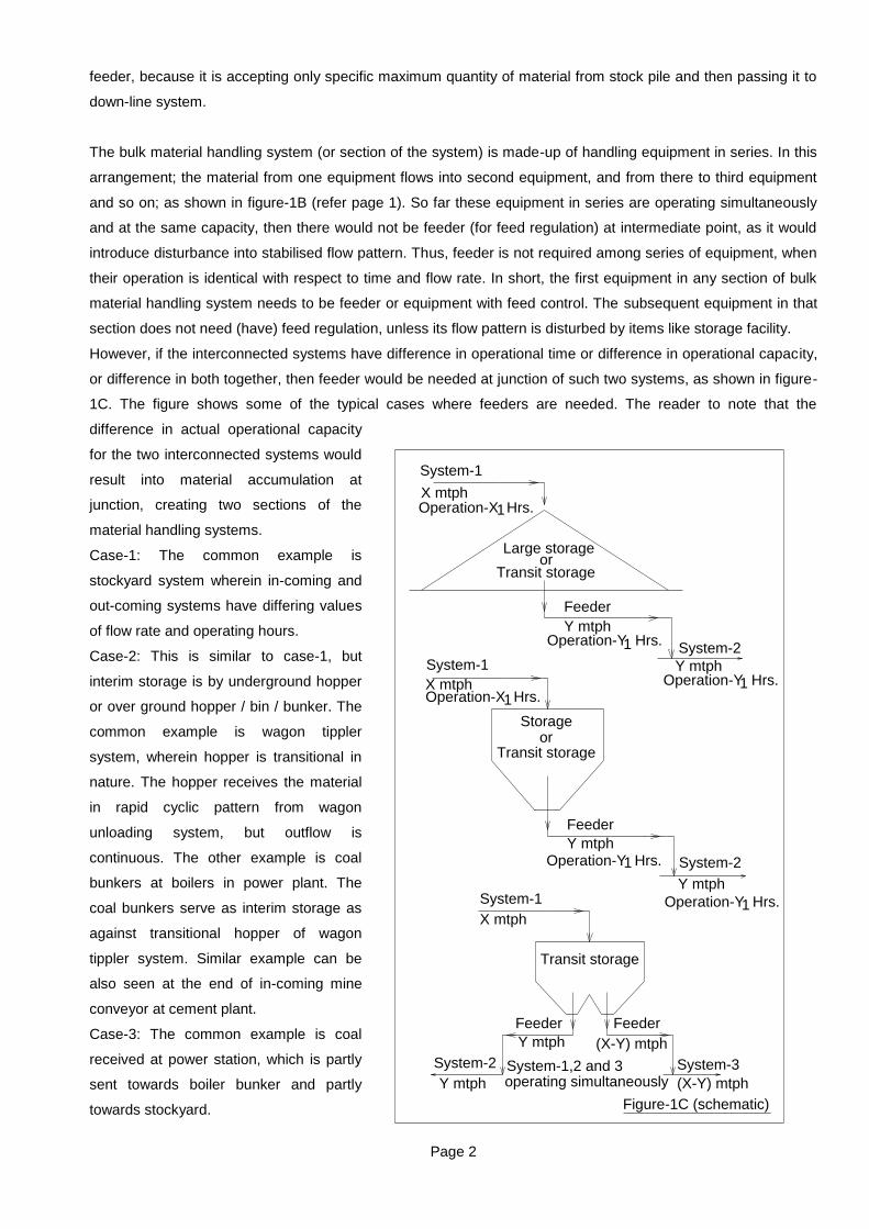
However, if the interconnected systems have difference in operational time or difference in operational capacity,
or difference in both together, then feeder would be needed at junction of such two systems, as shown in figure-
1C. The figure shows some of the typical cases where feeders are needed. The reader to note that the
difference in actual operational capacity
for the two interconnected systems would
result into material accumulation at
junction, creating two sections of the
material handling systems.
Case-1: The common example is
stockyard system wherein in-coming and
out-coming systems have differing values
of flow rate and operating hours.
Case-2: This is similar to case-1, but
interim storage is by underground hopper
or over ground hopper / bin / bunker. The
common example is wagon tippler
system, wherein hopper is transitional in
nature. The hopper receives the material
in rapid cyclic pattern from wagon
unloading system, but outflow is
continuous. The other example is coal
bunkers at boilers in power plant. The
coal bunkers serve as interim storage as
against transitional hopper of wagon
tippler system. Similar example can be
also seen at the end of in-coming mine
conveyor at cement plant.
Case-3: The common example is coal
received at power station, which is partly
sent towards boiler bunker and partly
towards stockyard.
System-1
X mtphOperation-X Hrs.1
1Operation-Y Hrs.Y mtph
Feeder
System-2
Y mtphOperation-Y Hrs.1
Large storage
Transit storage or
orTransit storage
Storage
1Operation-Y Hrs.
Y mtph
System-2
Feeder
Y mtphOperation-Y Hrs.1
1Operation-X Hrs.X mtph
System-1
System-1
X mtph
(X-Y) mtph
Feeder
System-3
(X-Y) mtph
Transit storage
Y mtph
System-2
Feeder
Y mtph
operating simultaneously
Figure-1C (schematic)
System-1,2 and 3
Page 3
1.2.0 TYPE OF FEEDERS
Various types of feeders have evolved during course of time, to suit differing needs of bulk material handling
plants. The different types of feeders are needed because bulk materials can range from food grains, coal,
minerals, granite, and so on which have altogether different physical characteristics. The different types of
feeders are also required to suit the need for large difference in capacity ranging from few mtph to mtph in
thousands. Mainly, following types of feeders are available for choice and needs:
1) Belt feeders
2) Apron feeders
3) Vibrating feeders (Electromagnetic)
4) Vibrating feeders (Mechanical)
5) Reciprocating feeders
6) Screw feeders
7) Drag chain / drag flight feeders
8) Rotary table feeders
9) Rotary van feeders
10) Rotary drum feeders
11) Rotary plough feeders
1.3.0 FEEDERS MAIN CHARACTERISTICS AND APPLICATION
1.3.1 Belt feeders
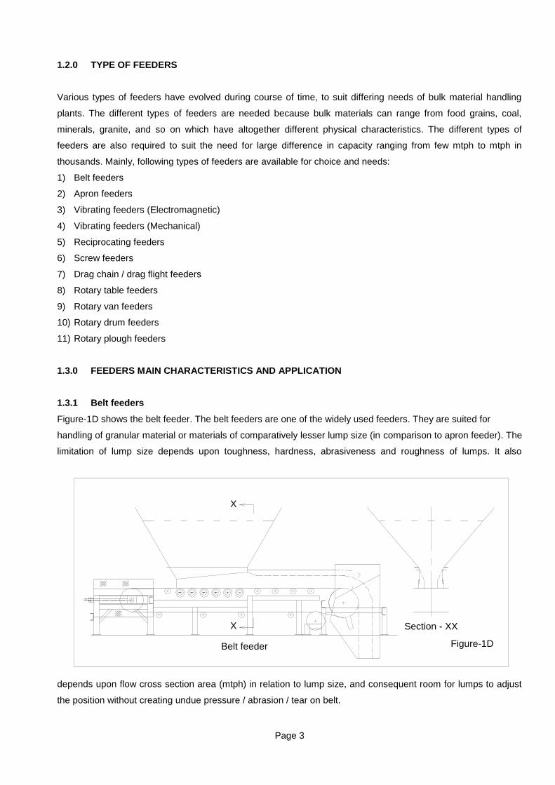
Figure-1D shows the belt feeder. The belt feeders are one of the widely used feeders. They are suited for
handling of granular material or materials of comparatively lesser lump size (in comparison to apron feeder). The
limitation of lump size depends upon toughness, hardness, abrasiveness and roughness of lumps. It also
depends upon flow cross section area (mtph) in relation to lump size, and consequent room for lumps to adjust
the position without creating undue pressure / abrasion / tear on belt.
Belt feeder
X
X Section - XX
Figure-1D
Page 4
The belt feeder is not recommended for very hard and tough material which have sharp cutting edges and
comparatively of large lumps (i.e. belt feeder is not substitute to apron feeder). It is difficult to quantify this issue
in simple or mathematical terms. In case of uncommon application, the designer has to check about the previous
use of belt feeder in somewhat comparable situation in existing plants or his previous experience. Regarding
basic rule for preliminary decision, the designer has to imagine that :
1) In case of large lumpy material, imagine that the lump/s are blocked momentarily (i.e. not moving with belt).
2) Lumps are pressing on belt due to pressure above and also additionally due to reshuffling reaction forces
when the belt is trying to dislodge the jammed lumps (by eliminating arch formation in plane of belt). Such
things continue to happen momentarily even without being observed.
3) In the situation stated above, imagine whether the sharp edges front part would get sheared off to make the
lump edges blunt. If these edges front line are getting blunted, or the pressure is not high enough to create
cut / puncture on belt, then belt feeder can suit.
4) In the situation stated above, imagine whether the sharp edges of lumps will get worn out by belt (also by
material particles on belt), to make them blunt. If the edges extreme front line get blunted immediately, or the
pressure is not high enough to create cut / puncture on belt, then belt feeder can suit the application.
5) If the points mentioned against serial number 3 and 4 are unfavourable; then the same can be overcome to
certain extent by providing thick top cover to belt, making the use of belt feeder possible.
The aforesaid guidelines help in engineering judgement. The belt feeder use for granular or material of limited
lump size, do not pose such dilemma.
The belt feeder can extract the material from hopper outlet. The hopper outlet length along feeder, can be up to
7 to 8 meters in favourable situation (lesser the feed zone length, more favorable is the situation for belt life).
The belt feeder center to center distance is different from this feed zone length. The virtual freedom in choosing
center to center distance of belt feeder, provides excellent flexibility for optimum layout of associated portion of
the plant.
The belt feeder discharge is positive volumetric in nature. The typical capacity range is up to 1500 m3/hour, for
regularly used belt widths. However, belt feeders of higher capacities are also possible. As an example, a mine
in Germany has 6400 mm wide belt feeder for handling lignite at much higher capacity.
1.3.2 Apron feeders
Figure-1E shows the apron feeder. The apron feeder is used for dealing with materials which are very hard,
abrasive, tough and for lumps of larger dimensions; which are beyond the scope of belt feeders. The boulders of
even 1.5 m edge length dimension can be handled, because such lumps will be falling and carried by steel pans,
which can have thickness of 6 mm to 40 mm. Again, at loading zone, the multiple support pads under the pans
can be provided to withstand the impact of such large lumps.
Page 5
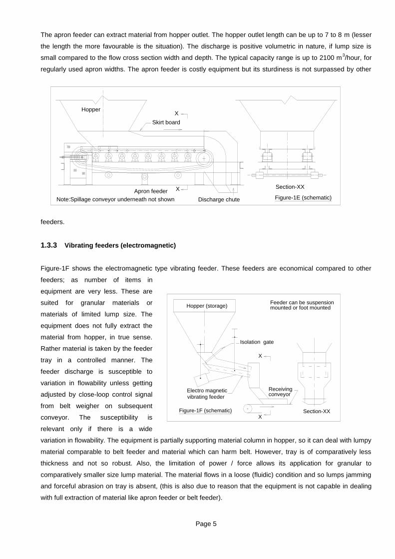
The apron feeder can extract material from hopper outlet. The hopper outlet length can be up to 7 to 8 m (lesser
the length the more favourable is the situation). The discharge is positive volumetric in nature, if lump size is
small compared to the flow cross section width and depth. The typical capacity range is up to 2100 m3/hour, for
regularly used apron widths. The apron feeder is costly equipment but its sturdiness is not surpassed by other
feeders.
1.3.3 Vibrating feeders (electromagnetic)
Figure-1F shows the electromagnetic type vibrating feeder. These feeders are economical compared to other
feeders; as number of items in
equipment are very less. These are
suited for granular materials or
materials of limited lump size. The
equipment does not fully extract the
material from hopper, in true sense.
Rather material is taken by the feeder
tray in a controlled manner. The
feeder discharge is susceptible to
variation in flowability unless getting
adjusted by close-loop control signal
from belt weigher on subsequent
conveyor. The susceptibility is
relevant only if there is a wide
variation in flowability. The equipment is partially supporting material column in hopper, so it can deal with lumpy
material comparable to belt feeder and material which can harm belt. However, tray is of comparatively less
thickness and not so robust. Also, the limitation of power / force allows its application for granular to
comparatively smaller size lump material. The material flows in a loose (fluidic) condition and so lumps jamming
and forceful abrasion on tray is absent, (this is also due to reason that the equipment is not capable in dealing
with full extraction of material like apron feeder or belt feeder).
Figure-1E (schematic)Apron feeder
Skirt board
Note:Spillage conveyor underneath not shown
Hopper
Discharge chute
X
X Section-XX
Figure-1F (schematic)
Receivingconveyor
Electro magnetic
vibrating feeder
Isolation gate
Hopper (storage)
X
XSection-XX
Feeder can be suspension mounted or foot mounted
Page 6
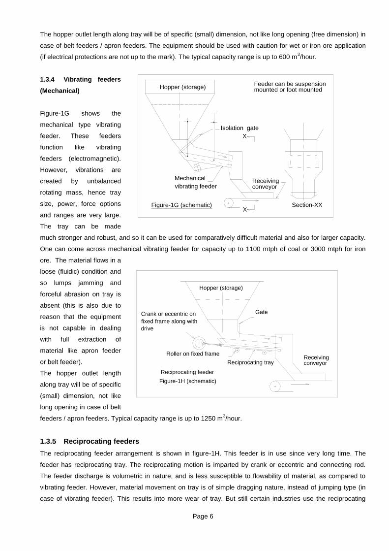
The hopper outlet length along tray will be of specific (small) dimension, not like long opening (free dimension) in
case of belt feeders / apron feeders. The equipment should be used with caution for wet or iron ore application
(if electrical protections are not up to the mark). The typical capacity range is up to 600 m3/hour.
1.3.4 Vibrating feeders
(Mechanical)
Figure-1G shows the
mechanical type vibrating
feeder. These feeders
function like vibrating
feeders (electromagnetic).
However, vibrations are
created by unbalanced
rotating mass, hence tray
size, power, force options
and ranges are very large.
The tray can be made
much stronger and robust, and so it can be used for comparatively difficult material and also for larger capacity.
One can come across mechanical vibrating feeder for capacity up to 1100 mtph of coal or 3000 mtph for iron
ore. The material flows in a
loose (fluidic) condition and
so lumps jamming and
forceful abrasion on tray is
absent (this is also due to
reason that the equipment
is not capable in dealing
with full extraction of
material like apron feeder
or belt feeder).
The hopper outlet length
along tray will be of specific
(small) dimension, not like
long opening in case of belt
feeders / apron feeders. Typical capacity range is up to 1250 m3/hour.
1.3.5 Reciprocating feeders
The reciprocating feeder arrangement is shown in figure-1H. This feeder is in use since very long time. The
feeder has reciprocating tray. The reciprocating motion is imparted by crank or eccentric and connecting rod.
The feeder discharge is volumetric in nature, and is less susceptible to flowability of material, as compared to
vibrating feeder. However, material movement on tray is of simple dragging nature, instead of jumping type (in
case of vibrating feeder). This results into more wear of tray. But still certain industries use the reciprocating
Section-XXX
X
Isolation gate
vibrating feeder
Mechanical
Figure-1G (schematic)
mounted or foot mountedFeeder can be suspension
conveyorReceiving
Hopper (storage)
Reciprocating feeder
Hopper (storage)
Gate
conveyorReceiving
Figure-1H (schematic)
Roller on fixed frame
fixed frame along with
Crank or eccentric on
Reciprocating tray
drive

Page 7
feeder. The magnitude of vibrating forces are comparatively high but at a very low frequency, say at about 60
cycle per minute. The commonly used reciprocating feeders have capacity range up to 250m3/hr, for material of
average abrasiveness. The higher capacities are possible. The feeder can handle larger lumps, compared to
vibrating feeder.
1.3.6 Screw feeders
Figure-1J shows the screw feeder. These feeders are suitable for material which are granular / powdery or which
have small size lumps (in tens of mm). The feeder extracts the material from hopper. It provides totally enclosed
construction from hopper to receiving equipment. The capacity range is less compared to earlier described
feeders.
The material continuously rubs with flights and trough. So, abrasive material will cause faster wear. The feeder is
extensively used in grain industries and for granular materials in process plants.
It is not used for materials which have tendency to pack or interlock and thereby difficult to shear or create flow.
It should also be used with caution where material is likely to solidify during idle time. Feeder is simple and
economical. The typical capacity range is up to 200 m3/hour
1.3.7 Drag chain / Drag flight feeders
Figure-1K shows the drag chain / drag flight feeder. The feeder extracts the material from hopper. It is suitable
for materials of moderate size lumps and of average abrasiveness. The hopper outlet can have some length
along feeder. It can provide enclosed construction. The feeder needs minimum installation heights, it also
imparts agitation to material at outlet, i.e. improves flow at hopper outlet. Typical capacity range is up to 100
m3/hour.
Section-XX X
XDrive end
Outlet
Hopper
Figure-1J (schematic)
Screw feeder

Page 8
1.3.8 Rotary table feeders
Figure-1L shows the rotary table feeder.
These feeders are suitable to install under
hopper outlet of larger diameter to prevent
clogging by sluggish material. The feeders
are suitable for non abrasive and marginally
abrasive materials. The material
continuously rubs / slides on table, however,
table can be fitted with thick liner if needed.
Discharge is volumetric in nature. The
capacity range is limited, say up to 20 m3/
hour.
1.3.9 Rotary vane feeders
Figure-1M shows the rotary vane feeder.
These feeders are particularly used to
discharge fine freely flowing material from
hopper, while maintaining sealing so that air
/ gases do not flow into hopper, when
hopper is under negative air pressure.
These feeders are regular features for
discharge of dust from dust collection
hopper / enclosure in a dust extraction
plant. These feeders can be also used when
such sealing is not required. The discharge is positive volumetric in nature. The other area of application can be
process plant, where material is to flow in a totally enclosed construction. The feeder is suitable for materials,
Drive
Figure-1L (schematic)
Section-XX
X
Stationary ring
Rotating disc
(skirt plate)
Rotary table feeder
Discharge barrier
X
Hopper
Discharge chute
Drag flight feeder
Figure-1K (schematic)
Control gate
Hopper
Drive end
Discharge end
Flow
Flow Flow

Page 9
which are free flowing and non-sticky. This feeder application competes with screw feeder, but this is not so
popular as screw feeder. However, if feeding is to be accomplished with minimum horizontal displacement, then
this feeder will be the choice.
1.3.10 Rotary drum feeders
Figure-1N shows the rotary drum feeder. This simple
and sturdy feeder is suitable for free flowing and small
lump material. It extracts the material from hopper. The
discharge is positive volumetric and accurate. This
feeder is not suitable for very abrasive materials in
continuous duty application. It is also not suitable for
sticky material. The material rubs continuously with
rotating periphery. The typical capacity range is up to
150 m3/hour.
1.3.11 Paddle feeders (or plough feeders or plow
feeders)
Figure-1P shows the paddle feeder. Generally, this is
travelling type and extracts material from hopper-shelf.
The feeder travel and thereby hopper outlet length can be up to 200m or so. This feeder is suitable to operate in
tunnel under stockpile. The feeder along with civil work is an expensive proposition, and is used to reclaim
material from track hopper or long stockpile on storage-yard. The feeder can deal with practically any material,
and in large capacity range. The feeder requirement in a particular layout arrangement is without alternative
option of matching performance. Thus, this feeder does not compete with other feeders, but competes with other
reclaiming machines. It is more as reclaiming machine-cum-feeder. The feeder extracts the material forcefully
and so, it can also deal with materials, which have tendency to pack or interlock. The typical capacity range is up
Figure-1N (schematic)
Rotary drum feeder
Hopper
Control gate
X
X
Rotary vane feederpowdery material lumpy material
Rotary vane feederSection-XX
Drive
Figure-1M (schematic)
X
X

Page 10
to 1250 m3/hour. More capacity is also possible. In general, this is used for lump size up to 450 mm. This
depends upon the characteristics of material.
Chapter 2: INTRODUCTION TO BELT FEEDER
This chapter has 7 pages. Following 2 pages write-up is typical.
BELT FEEDER FUNCTION
The purpose and function of belt feeder is to draw out specific quantity (m3/sec) of material from hopper, for
discharging in to onward system. The specific quantity could be as per pre-setting or as dictated by manual /
Hopper
X
X
Section-XX
Figure-1P (schematic)
Paddle feeder (or plough feeder or plow feeder)
travelMachine
Impacttable

Page 11
automatic command. The equipment like conveyor, crusher, screen, etc., if placed directly below hopper, same
will get flooded with material from hopper. This will result into overloading of this equipment, because this
equipment can not be provided with constructional feature for taking only set quantity of material (exception is
some crusher suitable for choke feed). In fact there would be chaos in entire system, in absence of feeder below
hopper.
The belt feeder is placed below the hopper. The belt feeder also gets flooded with material (choke feed).
However, it is designed to work in this condition and take only set quantity (m3/sec) of material, even though
more quantity of material is present in the hopper.
Referring to figure- 2A & 2B, the belt feeder skirt board is flange connected with the hopper outlet (or adapter
outlet). Thus, hopper skirt board and belt forms totally enclosed space. The material in the hopper has continuity
through skirt board, and rests (presses) directly on the belt, due to gravitational force.
Thus material is directly pressing on belt, all the time, and hence there exists frictional grip between belt and
material. In view of this frictional grip, the belt forward motion drags the material along with it. However, entire
body of material in hopper, can not move forward due to following reasons:
The belt motion tends to drag the body of material forward, but hopper (adapter) front wall acts as barrier
except for opening at exit end of hopper.
There is frictional grip between material and hopper / skirt walls, which opposes the material movement
forward.
The material body is subjected to forward forces by tractive pull and backward forces by frictional
resistances. This opposing force results in to shearing of material at weakest plane. Accordingly, part of
material in contact with belt moves forward, whereas balance material tends to be stationary.
Not withstanding the numerous intricacies of internal forces and internal movements within material, finally
the material quantity which is emerging out at hopper outlet front end is specific in accordance with front end
opening area and belt velocity. This is so, because material is being pulled out by belt, under choke feed
situation.
The material quantity Qv m3/sec drawn out from hopper, and which would be discharged by belt feeder at
head pulley is given by following formula:
Qv = (front end opening area m2) x (material cross section average velocity at this opening, m/sec).
The material cross section average velocity at hopper exit is subjective to specific application, on case to
case basis. This could be in the range of 0.70 to 0.85 of belt velocity. As a general statement, considering
this to be 0.75 of belt velocity, the formula can be written as below:
Qv = (front end opening area m2) x [(belt velocity m/sec) x 0.75]
= (skirt inside width at exit) x [(opening height at exit) x 0.75] x (belt velocity) m3/sec
The above formula clarifies the basic functional nature of belt feeder discharge. For more clarity, refer chapter-6
and chapter-7.
It is evident from this formula that Qv is volumetric in nature and can be adjusted by front end opening area or by
adjustment in belt velocity. Accordingly, the belt discharge rate is controlled as below:
1) The control gate (i.e. front end opening height adjustment gate / slide plate) is always provided in belt
feeder. This enables to manually change the opening height and thereby flow area at exit section. This is
widely used to control flow rate for many of the feeders dealing with granular material or when lump size is
not large, and when push button adjustment is not needed.

Page 12
2) The variable speed drive enables to vary the feeder discharge because discharge is directly proportional to
belt velocity. So slower speed is used for lesser discharge, and faster speed for more discharge. The
operator makes the speed setting to suit required discharge. Thus this arrangement enables push button
control of discharge rate. The variable speed drive can be also used for automatic control of belt speed so
as to have set value of discharge rate (mtph), by electrical inter-lock with belt weigher on subsequent
conveyor.
Most of the time belt feeders are set to discharge specific m3/sec. In case one is trying to change the discharge
rate frequently, the following aspects and limitation of the whole system should be taken in to consideration:
Hopper filling rate multiplied by filling duration, in certain time cycle.
The hopper should have enough storage capacity to balance out its inflow and outflow, in the aforesaid time
cycle. In short, feeder discharge rate should not be changed arbitrarily; ignoring the hopper inflow cycle,
hopper storage capacity and hopper outflow (feeder discharge). Otherwise, this can result into flow
imbalance and system tripping and non-workable system.
As said before, belt feeder discharge rate is volumetric in nature and this can be converted in to mtph as
below.
The feeder discharge rate in mtph = (volumetric discharge m3/sec) x 3600 x (bulk density kg/m
3) 1000 =
3.6 x (volumetric discharge m3/sec) x (bulk density kg/m
3) mtph
Chapter 3: BULK MATERIALS
This chapter has 10 pages. Following 1 page write-up is typical.
Table-2 : Common materials repose angle and wall friction coefficient
Note : 1) The table-2 indicates average values. These can vary as per source. Use specific values for
contractual needs.
2) Case-1 s : This is applicable to plain and fairly even surface of steel, aluminum, average plastic; without
protruding edges. Flush and welded steel surface would be of this type.
3) Case-2 s : This is applicable to surface of medium smoothness / evenness, such as welded steel flush
surface (below average), smooth concrete, wood planks, protruding edges, bolt head rivets etc.
4) The designer can also use s value in between case-1 and case-2. This data is not applicable to corrugated
surface.
Case-1 Case-2 Case-1 Case-2
Ash fly 41 0.50 0.60 Lignite (dry) 37 0.475 0.55
Barley 24 0.25 0.35 Limestone 37 0.42 0.50
Cement clinker 44 0.45 0.55 Limestone, fines 38 0.40 0.50
Cement portland
(non-aerated)37 0.40 0.45 Maize 34 0.23 0.36
Coal bituminous 36 0.44 0.49 Sand dry 37 0.38 0.48
Coal bituminous, fines 41 0.40 0.50 Slag clinker 38 0.50 0.60
Coke 35 0.50 0.55 Soya beans 27 0.25 0.38
Granite, blackish
(-) 75 mm38 0.47 0.57 Sugar 37 0.45 0.50
Gravel (river) 37 0.40 0.48 Wheat 30 0.24 0.38
Iron Ore Pellets 36 0.50 0.55
Repose
Angle
degrees
Material and surface
friction coefficient s
Material and surface
friction coefficient s Material
Repose
Angle
degrees
Material
Page 13
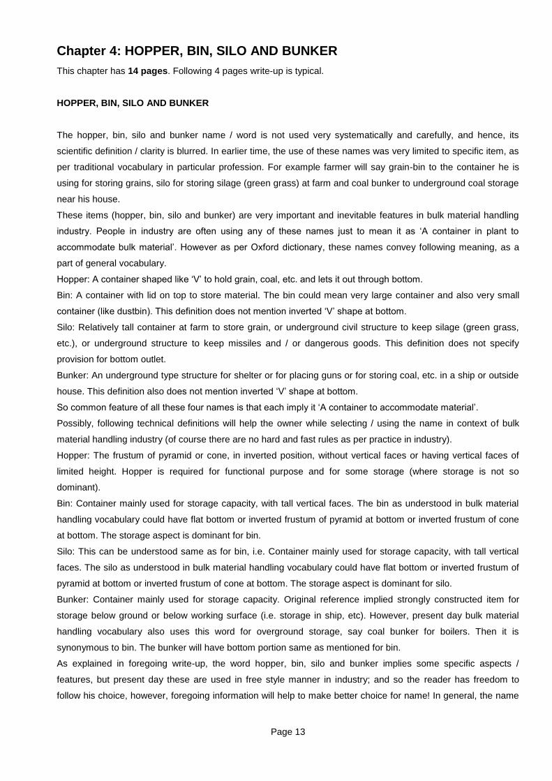
Chapter 4: HOPPER, BIN, SILO AND BUNKER
This chapter has 14 pages. Following 4 pages write-up is typical.
HOPPER, BIN, SILO AND BUNKER
The hopper, bin, silo and bunker name / word is not used very systematically and carefully, and hence, its
scientific definition / clarity is blurred. In earlier time, the use of these names was very limited to specific item, as
per traditional vocabulary in particular profession. For example farmer will say grain-bin to the container he is
using for storing grains, silo for storing silage (green grass) at farm and coal bunker to underground coal storage
near his house.
These items (hopper, bin, silo and bunker) are very important and inevitable features in bulk material handling
industry. People in industry are often using any of these names just to mean it as „A container in plant to
accommodate bulk material‟. However as per Oxford dictionary, these names convey following meaning, as a
part of general vocabulary.
Hopper: A container shaped like „V‟ to hold grain, coal, etc. and lets it out through bottom.
Bin: A container with lid on top to store material. The bin could mean very large container and also very small
container (like dustbin). This definition does not mention inverted „V‟ shape at bottom.
Silo: Relatively tall container at farm to store grain, or underground civil structure to keep silage (green grass,
etc.), or underground structure to keep missiles and / or dangerous goods. This definition does not specify
provision for bottom outlet.
Bunker: An underground type structure for shelter or for placing guns or for storing coal, etc. in a ship or outside
house. This definition also does not mention inverted „V‟ shape at bottom.
So common feature of all these four names is that each imply it „A container to accommodate material‟.
Possibly, following technical definitions will help the owner while selecting / using the name in context of bulk
material handling industry (of course there are no hard and fast rules as per practice in industry).
Hopper: The frustum of pyramid or cone, in inverted position, without vertical faces or having vertical faces of
limited height. Hopper is required for functional purpose and for some storage (where storage is not so
dominant).
Bin: Container mainly used for storage capacity, with tall vertical faces. The bin as understood in bulk material
handling vocabulary could have flat bottom or inverted frustum of pyramid at bottom or inverted frustum of cone
at bottom. The storage aspect is dominant for bin.
Silo: This can be understood same as for bin, i.e. Container mainly used for storage capacity, with tall vertical
faces. The silo as understood in bulk material handling vocabulary could have flat bottom or inverted frustum of
pyramid at bottom or inverted frustum of cone at bottom. The storage aspect is dominant for silo.
Bunker: Container mainly used for storage capacity. Original reference implied strongly constructed item for
storage below ground or below working surface (i.e. storage in ship, etc). However, present day bulk material
handling vocabulary also uses this word for overground storage, say coal bunker for boilers. Then it is
synonymous to bin. The bunker will have bottom portion same as mentioned for bin.
As explained in foregoing write-up, the word hopper, bin, silo and bunker implies some specific aspects /
features, but present day these are used in free style manner in industry; and so the reader has freedom to
follow his choice, however, foregoing information will help to make better choice for name! In general, the name

Page 14
mentioned by buyer becomes the name of the item in particular plant. The foregoing lengthy elaboration about
name is not for hypothetical reasons, but directly concerns what name to be used here.
As for the issue of using name in this book; the situation is as below:
The bulk material storage container in bulk material handling plant will always have bottom discharge outlet and
equipment at bottom. So, the hopper aspect is present most of the time and it should prevail. Thus, the right
word for such storage container would be hopper, or (hopper + bin) or (hopper + silo) or (hopper + bunker).
However using such theoretically correct name would make the presentation difficult and also uncomfortable for
the reader. So, only one word hopper has been used in this book in following manner.
- Word hopper is used in this book to mean the complete container for storing material. The hopper of
this book can have only converging portion or converging portion + vertical portion.
- To describe the engineering phenomenon or formula applicable to particular region of hopper, the issue has
been addressed in this book by using words such as ‘hopper vertical portion’ or ‘hopper converging
portion’.
It would be better if reputed standards promote the use of only single name (for complete container) in bulk
material handling industry, because dictionary meanings of various original names have artistic angle for
sophisticated expressions, but the same are not relevant for bulk material handling industry today. Because
these items are being used for storing all sorts of materials, ranging from iron ore pellets, minerals, fertilisers,
salts and so on, which are at variance to original reference to hopper, bin, silo and bunker.
HOPPER FUNCTIONS
The hopper/s are
inevitable items in most
of the plants for
handling of bulk
materials. The hopper
is needed at the
junction of two systems
which have different
values of instantaneous
flow rates (m3/sec), and
system themselves are
not capable to absorb /
cushion-out this
difference in flow rate.
Example-1
Calculate the gross and maximum effective capacity of hopper as shown in figure-4K. The material inside
hopper is coal of (-) 50mm size, bulk density 0.8 t/m3, repose angle 35. The material filling at top in area
2m x 2m at center.
Flow rate fluctuating
0 to 3 tonne / minute
System-1 Hopper System-2
1tonne / minute
Flow rate steady
System-1
System-2
210 3 4 5
1
2
3
Figure-4ATime in minute
Tonne / minute

Page 15
Solution
The material maximum filling in hopper will be as shown in figure-4K. The filled volume to be divided into known
shapes to enable
calculation of capacity. The
material from top face of
2m x 2m will spread
laterally as per 35 repose
angle. As the hopper cross
section is rectangle, the
sloping faces will intersect
to two vertical faces as
shown.
The material spread from
each corner of top square
will form conical surface.
There will be 4 nos. of
quarter cones i.e. all
together will form one cone.
However, these quarter
cones base will not be flat
but will be curved up-down-
up in accordance with cone
curved surface intersection
with vertical planes at
differing horizontal
distance.
The hopper converging
portion (imagine views
without dotted extension
lines below bottom outlet)
would look like frustum of
pyramid, but closer study
shows it is not frustum of
pyramid. All the four edges are appearing in plan view but are not meeting at common point. If these four edges
are meeting at common point, then these would also appear meeting at common point in plan view; because
view of the point is same from any angle. This would be more clear by extending elevation and end view, below
bottom outlet, as shown in dotted lines. These dotted lines are meeting at different place, in elevation and end
view. So, converging portion is not frustum of pyramid. Instead it is frustum of wedge. The bottom converging
portion volume can be computed as wedge of 3.4641 + 0.8659 = 4.33 m height minus wedge of 0.8659 m
height. The material fill-up volume is as below, as per foregoing explanation.
Portion (1), cuboid = 2 x 2 x (1.05 + 0.70) = 7.0 m3
Portion (2), prism = 0.5 x 2.5 x 1.75 x 2 = 4.375 m3
Figure-4K
4.5m
3.4641m1.5m1.5m
1m 1m
60°
3.5m
1m 1m
7
6
2 1 2A
3.5m
A B
2
3
1 2A
3A 5C5D
5A 5B
3.5m3.5m
View-YY
YY
ZZ
X
X
View-ZZ
3.5m 3.5m
4A
6
60°
2.5m 2.5m
1m 1m
1
3A3
4C D
0.75m
1.05m
0.70m
2m
3.4641m
0.8659m
0.5m0.5m
View-XX
Front view
7

Page 16
Portion (2A), prism = 0.5 x 2.5 x 1.75 x 2 = 4.375 m3
Portion (3), prism = 0.5 x 1.5 x 1.05 x 2 = 1.575 m3
Portion (3A), prism = 0.5 x 1.5 x 1.05 x 2 = 1.575 m3
Portion (4), cuboid = 1.5 x 0.7 x 2 = 2.10 m3
Portion (4A), cuboid = 1.5 x 0.7 x 2 = 2.10 m3
The four nos. of cone quadrant will make one cone. So, volume of one cone is computed. Looking to plan view,
the base radius can be considered approximately as an average of (2.5 - 1.0) + (3.5 - 1.0) + diagonal = 1.5 + 2.5
+ diagonal.
Its average height as 0.5 x [1.05 + (1.05 + 0.7)] = 1.4 m
Portion (6), cuboid = 5 x 7 x 2 = 70 m3
Hence maximum effective volume :
=7.0 + 4.375 + 4.375 + 1.575 + 1.575 + 2.10 + 2.10 + 7.785 + 70 + 56.579 = 157.464 m3
Gross volume = 5 x 7 x 4.5 + 56.579 = 214.079 m3
Chapter 5: BELT SPEED AND CAPACITY FOR BELT FEEDER
This chapter has 24 pages. Following 5 pages write-up is typical.
BELT SPEED
Selecting the optimum belt speed is very important step in design of belt feeder. The belt feeder performance,
life and price depend upon belt speed. The belt speed selection requires thoughtful understanding of bulk
material characteristics and its action on belt described in foregoing cl.-5.4.1 to cl.-5.4.5. The belt speed is
influenced by following points:
- The belt speed is less for material of higher abrasion capability. The belt speed is more for material of less
abrasion capability.
The material abrasion capability is in proportion to total abrasion factor Aft. The total abrasion factor
Aft = General abrasion Af + Lump factor Lf
- The belt speed being used is somewhat less for heavy bulk material. This is due to reason that for same
column height, the material force (pressure) and belt abrasion is more in case of heavy material. The
material column height is same for equal values of friction angles, equal values of external features of lumps
/ granules and hopper arrangement; but independent of bulk density. So density aspect is to be incorporated
in belt speed calculation. This influence is accounted by factor Df.
m305.23
5.25.15.25.1
radiusAveage
22
32 m785.7305.2xx4.1x3
1cone),D5()C5()B5()A5(Portion
3m579.56154.1733.576
233x1x8659.0
6
277x5x33.4)7(Portion

Page 17
- The belt speed is comparatively less for difficult feed zone and is more for easy feed zone. This is due to
consideration that the difficult feed zone results into more abrasion / wear of belt. This influence is
accounted by feed zone factor Ff.
The belt speed basic formula is as below, in considerations to above influences (also refer page-56).
The reader would be interested to know about the mentioned belt speed formula. This is based on following
benchmarks:
Belt speed of about 0.075 mps (15 fpm) is used in applications dealing with most difficult material and most
difficult feed zone i.e. worst situation as permitted for belt feeder.
Belt speed of about 0.5 mps (100 fpm) is used in applications dealing with very easy materials and easy
feed zone.
The observed speed values in practice for some of the intermediate materials.
The formula provides speed within this range in accordance with the application conditions.
The belt speed calculation always involves certain element of subjectivity, because most suitable speed will
depend upon the exact nature of material and belt feeder hopper arrangement, which are specific to application.
This should be given open thought and in case of doubt, opt for somewhat lower speed. The past experience /
data, if available, should also be utilised in problems pertaining to application engineering.
The belt feeder located in constrained space (like mobile equipment) can have speed more than calculated, but
same amounts to reduced life, as no option.
For grain like wheat, rice, etc., Aft is zero for use in this formula, which provides belt speed of 0.5 mps as an
average value for grain. However, somewhat higher speed can be used for gain if material pressure is not very
high (i.e. if hopper is not very deep).
The required input to this formula are described as below:
Abrasion total factor Aft
This factor is sum of following factors:
Aft = abrasion factor Af + lump factor Lf.
The value of Af is to be decided using table-3. This table mentions value of Af for model materials. Now, actual
material to be handled by belt feeder may not be mentioned in this table. In such situation, compare the
conventional abrasiveness of actual material with the listed material. The Af value of best matching material will
also be Af value of actual material. The designer can also select intermediate value, in accordance with relative
comparison.
The abrasive gradation such as A1, A2, A3, A4 or 6, 7, 8, 9, etc. are easily available for most of the materials,
from published literature. This abrasive gradation provides easy guide to decide value of Af. However, visual
inspection of material for refinement of decision is recommended for application and contractual design.
Similarly value of Lf is to be decided using graphs of figure-5D. The graph mentions value of Lf for model
materials. So, actual material to be handled by belt feeder may not be mentioned in this graph. In such case
mpsFf.Df.
100
Aft100x4.01.0
mpsFf.Df.100
Aft100x1.05.01.0vspeedBelt

Page 18
compare the abrasion / attrition capability of lumps of actual material, to the attrition capability of lumps of model
material. The Lf value of best matching material will also be Lf value of actual material. The designer can also
select the intermediate value, in accordance with relative comparison. The above mentioned lump attrition
capability implies the lump capability to inflict abrasion / wear / deterioration of belt as a combined effect of lump
hardness, lump toughness and sharp edges / corners on lump, as described under cl.-5.4.4.
Coming to the practical aspect of comparison of lump factor; it is necessary that the designer should see the
actual material and also the model materials, to enable him to make correct judgement. The listed model
materials like wheat, lignite, coal, limestone, cement clinker, granite, etc. are so common that the engineer with
very little exposure to bulk material handling will come across and see these materials. It is possible that such
materials might have been already seen in day to day life without specific exposure. As for the actual material,
one can ask for sample or alternatively refer to published information on such material. Or reference should be
made to buyer / producer to provide physical characteristics and description as to how it compare to model
materials on concerned aspects. The experienced engineer can make comparative decision on visual inspect,
because such decision relates to only one issue i.e. how good / bad is material lump for damage / abrasion
to belt.
The other alternative option is to ask for numerical values of hardness, toughness, etc. of lumps which demands
testing of reasonable number of sample. This is expensive and time consuming. Thus , values of Af and Lf are
decided as explained in foregoing write-up. The value of Aft is:
Aft = Af + Lf.
Bulk density factor Df
Df = 1.0 if material bulk density 1000kg/m3
Df = 0.95 if 1000 kg/m3 Bulk density of material 1650 kg/m
3 (i.e. when bulk density is more than
1000 kg/m3, and up to 1650 kg/m
3.
Feed zone factor Ff
This factor depends upon skirt board arrangement, feed zone length, feed zone width and lump factor. Thus it is
inter dependent on lump factor also. This is due to reason that the difficult lumpy material and difficult feed zone
combine effect is “geometric (more than proportionate)” in nature.
The values of feed zone factor Ff are as below:
Most easy or easy feed zone Lf 25 : Ff = 1.0
Most easy or easy feed zone Lf 25 : Ff = 0.90
Difficult feed zone Lf 25 : Ff = 0.90
Difficult feed zone Lf 25 : Ff = 0.80
Most difficult feed zone Lf 25 : Ff = 0.85
Most difficult feed zone Lf 25 : Ff = 0.75
The aforesaid values are primarily for industrial materials. In case of gains like wheat, rice, etc., Ff can be
considered generally as 1.0 or in very adverse conditions as 0.9.
Thus to decide Ff, one has to decide lump factor Lf and feed zone type i.e. whether easy type, difficult type,
more difficult type, etc.
The lump factor Lf is known as per clause 5.4.5.
Referring to figure-5E, the decision for feed zone type whether most easy, easy, difficult or most difficult;
requires relative value of L and W, which are yet not known (in fact the exercise is to find the values of L and W).
To circumvent this obstacle, consider feed zone arrangement at midway, say „difficult‟, while making first time

Page 19
calculation, and decide Ff accordingly. Use this Ff value to calculate preliminary belt speed. Thus, having
decided the preliminary belt speed, the preliminary value of W becomes known as per clause-5.7.0. This
becomes an input to next stage design process, to derive real value of W. This is the standard process of first
stage design becoming input to second stage design to reach the final value. The design procedure will be clear
from the example.
Firstly, decide the preliminary elevation view of the proposed arrangement for belt feeder, as shown in following
figure-5E, (depiction is as per scale).
The belt feeder feed zone arrangement can be as per any one of the arrangement in figure-5E. These
arrangements elevation views (feed zone length) depends upon technical requirements such as starting point of
belt feeder, ending point of belt feeder, feed zone length to suit dimensional constrain, hopper outlet size, etc.
These are already known to suit the overall plant arrangement. The preliminary value of W is already decided as
mentioned in foregoing write-up Hence preliminary plotting or assessing of the applicable arrangement is
possible (This refers to only preliminary arrangement). This would enable to decide second stage value of Ff.
Having decided the value of Af, Lf, Aft, Df and Ff as explained in foregoing write-up, calculate the belt speed v as
below:
Above calculated speed when equal or larger than approximately 0.125 mps (25 fpm), the same to be amended
by following factors, if applicable.
Material pressure factor 1.0; for C2 2.25.
OR material pressure factor 0.925; for 2.25 < C2 3.5
OR material pressure factor 0.85; for 3.5 < C2 4.5.
Lump numerical dimension factor 0.95; for lump dimension 170 mm.
OR Lump numerical dimension factor 0.9; for lump dimension > 250 mm, subjects to experience.
Figure-5E
L
L L
L
L L
X
X
X
X
X
X
X
X
X
X
X
X
W
Section-XXMost easy feed zone Easy feed zone
Easy feed zone Difficult feed zone
Difficult feed zone Most difficult feed zone
( 3 W L 5 W )
( L 5 W )( L 5 W )
( L 3 W ) ( L 2.5 W )
( 3 W L 5 W )
mpsFf.Df.
100
Aft100x4.01.0vspeedBelt

Page 20
The pressure factor C2 is for dynamic (continuous operation) condition. Refer chapter-8, cl.-8.14.4, page- 206,
for definition of C2.
The above factors are as per engineering judgement and the designer can adopt this speed or review / refine
this value on the basis of his specific experience and other data.
EXAMPLES - 1 TO 7
Decide the belt speed for wheat, lignite, coal less hard, hard coal, limestone less hard, hard limestone, and
granite, for following situations.
- Lumps of good shape, maximum size
- Lumps of good shape, 1/2 maximum size
- Lumps of good shape,1/4 maximum size
- Lumps of bad shape, maximum size
- Lumps of bad shape, 1/2 maximum size
- Lumps of bad shape,1/4 maximum size
Decide the above speed considering easy feed zone to belt feeder, and also considering difficult feed zone to
belt feeder. The material bulk densities are as below :
Wheat : 770 kg/m3
Lignite : 800 kg/m3
Coal less hard : 800 kg/m3
Coal hard : 800 kg/m3
Limestone less hard : 1400 kg/m3
Hard limestone : 1400 kg/m3
Granite : 1440 kg/m3
Following example -5 and 7 have only been presented here.
Example - 5 : limestone, less hard :
Referring to table-3 and graph figure-5D, the values of Af and Lf are as below :
The value of Af = 24
Lf = 27 (Maximum size and good lumps)
Lf = 21 (½ Maximum size and good lumps)
Lf = 17 (¼ Maximum size and good lumps)
Lf = 38 (Maximum size and bad lumps)
Lf = 27 (½ Maximum size and bad lumps)
Lf = 21 (¼ Maximum size and bad lumps)
The bulk density factor Df = 0.95, as density is greater than 1000 kg / m3
For Lf less than or equal to 25, the feed zone factor Ff = 1.0, for easy feed zone.
For Lf less than or equal to 25, the feed zone factor Ff = 0.9, for difficult feed zone.
For Lf greater than 25, the feed zone factor Ff = 0.9, for easy feed zone.
For Lf greater than 25, the feed zone factor Ff = 0.8, for difficult feed zone.
The belt speed values in different situations are as below:
Maximum size, good lumps, easy feed, v = [0.1 + 0.4 x (100 - 24 - 27) 100] x 0.95 x 0.9 = 0.2531mps
Page 21
Maximum size, good lumps, difficult feed, v = [0.1 + 0.4 x (100 - 24 - 27) 100] x 0.95 x 0.8 = 0.2249 mps
½ Maximum size, good lumps, easy feed, v = [0.1 + 0.4 x (100 - 24 - 21) 100] x 0.95 x 1 = 0.304 mps
½ Maximum size, good lumps, difficult feed, v = [0.1 + 0.4 x (100 - 24 - 21) 100] x 0.95 x 0.9 = 0.2736 mps
¼ Maximum size, good lumps, easy feed, v = [0.1 + 0.4 x (100 - 24 - 17) 100] x 0.95 x 1 = 0.3192 mps
¼ Maximum size, good lumps, difficult feed, v = [0.1 + 0.4 x (100 - 24 - 17) 100] x 0.95 x 0.9 = 0.2872 mps
Maximum size, bad lumps, easy feed, v = [0.1 + 0.4 x (100 - 24 - 38) 100] x 0.95 x 0.9 = 0.2154 mps
Maximum size, bad lumps, difficult feed, v = [0.1 + 0.4 x (100 - 24 - 38) 100] x 0.95 x 0.8 = 0.1915 mps
½ Maximum size, bad lumps, easy feed, v = [0.1 + 0.4 x (100 - 24 - 27) 100] x 0.95 x 0.9 = 0.253 mps
½ Maximum size, bad lumps, difficult feed, v = [0.1 + 0.4 x (100 - 24 - 27) 100] x 0.95 x 0.8 = 0.2249 mps
¼ Maximum size, bad lumps, easy feed, v = [0.1 + 0.4 x (100 - 24 - 21) 100] x 0.95 x 1 = 0.304 mps
¼ Maximum size, bad lumps, difficult feed, v = [0.1 + 0.4 x (100 - 24 - 21) 100] x 0.95 x 0.9 = 0.2736 mps
The above calculated speeds are to be multiplied by pressure factor and lump numerical dimension factor, if
applicable. In general lumps would be somewhat “bad”.
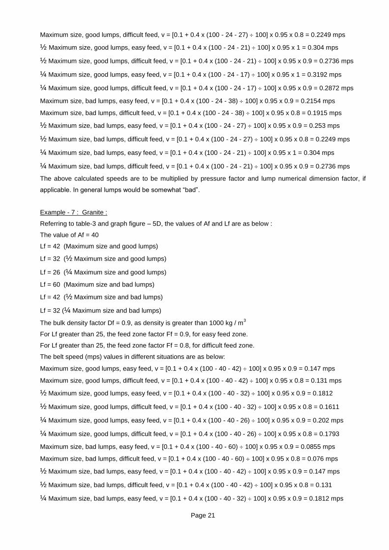
Example - 7 : Granite :
Referring to table-3 and graph figure – 5D, the values of Af and Lf are as below :
The value of Af = 40
Lf = 42 (Maximum size and good lumps)
Lf = 32 (½ Maximum size and good lumps)
Lf = 26 (¼ Maximum size and good lumps)
Lf = 60 (Maximum size and bad lumps)
Lf = 42 (½ Maximum size and bad lumps)
Lf = 32 (¼ Maximum size and bad lumps)
The bulk density factor Df = 0.9, as density is greater than 1000 kg / m3
For Lf greater than 25, the feed zone factor Ff = 0.9, for easy feed zone.
For Lf greater than 25, the feed zone factor Ff = 0.8, for difficult feed zone.
The belt speed (mps) values in different situations are as below:
Maximum size, good lumps, easy feed, v = [0.1 + 0.4 x (100 - 40 - 42) 100] x 0.95 x 0.9 = 0.147 mps
Maximum size, good lumps, difficult feed, v = [0.1 + 0.4 x (100 - 40 - 42) 100] x 0.95 x 0.8 = 0.131 mps
½ Maximum size, good lumps, easy feed, v = [0.1 + 0.4 x (100 - 40 - 32) 100] x 0.95 x 0.9 = 0.1812
½ Maximum size, good lumps, difficult feed, v = [0.1 + 0.4 x (100 - 40 - 32) 100] x 0.95 x 0.8 = 0.1611
¼ Maximum size, good lumps, easy feed, v = [0.1 + 0.4 x (100 - 40 - 26) 100] x 0.95 x 0.9 = 0.202 mps
¼ Maximum size, good lumps, difficult feed, v = [0.1 + 0.4 x (100 - 40 - 26) 100] x 0.95 x 0.8 = 0.1793
Maximum size, bad lumps, easy feed, v = [0.1 + 0.4 x (100 - 40 - 60) 100] x 0.95 x 0.9 = 0.0855 mps
Maximum size, bad lumps, difficult feed, v = [0.1 + 0.4 x (100 - 40 - 60) 100] x 0.95 x 0.8 = 0.076 mps
½ Maximum size, bad lumps, easy feed, v = [0.1 + 0.4 x (100 - 40 - 42) 100] x 0.95 x 0.9 = 0.147 mps
½ Maximum size, bad lumps, difficult feed, v = [0.1 + 0.4 x (100 - 40 - 42) 100] x 0.95 x 0.8 = 0.131
¼ Maximum size, bad lumps, easy feed, v = [0.1 + 0.4 x (100 - 40 - 32) 100] x 0.95 x 0.9 = 0.1812 mps

Page 22
¼ Maximum size, bad lumps, difficult feed, v = [0.1 + 0.4 x (100 - 40 - 32) 100] x 0.95 x 0.8 = 0.1611
The above calculated speeds are to be multiplied by pressure factor and lump numerical dimension factor, if
applicable. In general lumps would be “bad”.
Chapter 6: BELT FEEDER CROSS SECTION FEATURES
This chapter has 34 pages. Following 7 pages write-up is typical.
6.5.0 BELT FEEDER CROSS SECTION DETAILS (BEYOND FEED ZONE)
This topic establishes the main technical data / features for belt feeders, for cross section in conveying zone i.e.
beyond feed zone. Finally, this data have been summarised in table-4, table-5 and table-6. Most of the reasons
for this data have been already explained in preceding part of the chapter, and some of the reasons would be
clear, as the book progresses.
The conveying zone cross section fundamental parameters viz. material layer width (skirt board width), and
height values have been already analysed in foregoing cl. 6.2.0, cl.6.3.0 and 6.4.0. These values become
important input for the exercise here.
6.5.1 Picking type belt feeder cross section features (conveying zone)
The cross section of this belt feeder is shown in figure-6R. The aim of this exercise is to decide the values of all
dimensions appearing in this figure-6R.
Input data :
B: Belt width in mm. This is fixed during belt feeder design.
Lp : Pulley face width in mm. This is as per ISO / DIN in accordance with belt width.
Emin : Minimum edge margin in mm. This is the distance from outside of skirt rubber to belt edge, when belt has
maximum allowable misalignment. This value is decided considering functional needs, as explained under cl.
6.2.0. The numerical values of Emin are mentioned in table-4, and are to be used as input for this exercise.
y : The distance between skirt rubber outside to belt bending point (belt kink), theoretical, in mm. This value has
been selected as stated in table. The belt will have radial shape at theoretical bending point. This radial shape
will have minimum natural dimension, when being pressed by material. It is advisable that skirt rubber should be
some what away from this bending point, so that there would not be undue pressure between belt and skirt
rubber, when belt is empty. This value depends upon thickness / stiffness of belt, and designer should decide
W
Belt symetrical
Wn
tr
Wr
hsk
Rm
Bm
Rs
Bisy yy Bisyh
Rs Rs
hBiminy yBimax
Rs
Bm
Rm
hsk
Wr
tr
Wn
W
Belt misaligned (max)
Figure - 6R

Page 23
this value as per need. The values indicated in table are for average condition. More value of y is better for belt,
but it reduces the skirt board width and cross section area. The listed values are compromise of conflicting
needs between more room for the belt radius and reduction in cross section.
ts : skirt plate thickness in mm. This has been mentioned in table for average conditions. The designer can
review this as per his choice and its implication on other parameters.
tl : Thickness of liner on skirt plate in mm. This has been mentioned in table for average conditions. The
designer can review this as per his choice and its implication on other parameters.
tr : Skirt rubber thickness, 16 mm as an average.
h : Material layer height in skirt board, mm (conveying zone), as a factor (ratio) of W, such as 0.58 W, 0.65 W,
0.71 W etc. as decided by designer.
Output
The aforesaid input data enables to derive following output values in accordance with geometric reasons. Refer
figure-6R. Please note that for picking type belt feeder, the roller dimensions are fixed in this exercise to suit
their function in belt feeder. The arbitrary dimensional values of picking type idlers should not be mixed up here
i.e. values used for picking type conveyor are for different purpose, and need not be valid here.
Wn = 2B - Lp - 2 . Emin - 2 . tr = 2B - Lp - 2 . Emin - 32 mm (as per formula in cl.6.3.1 )
Wr = Wn + 2 . tr = Wn + 32 mm
W = Wn - 2 . ts - 2 . tl mm
Bm = Wr + 2 .y mm (Bm is belt flat portion, theoretical).
Bisy = (B - Bm) 2 mm (Bisy is inclined belt width, when belt is symmetrical).
Bimin = Emin - y mm (Bimin is inclined belt width, minimum, when belt is misaligned)
Bimax = B - Bm – Bimin mm (Bimax is inclined belt width, maximum, when belt is misaligned)
Emin = Bimin + y mm (This is actually input data).
Emax = Bimax + y mm (This is maximum edge margin when belt is misaligned)
Esy = Bisy + y mm (Belt edge margin when belt is symmetrical on idlers)
Rm = Bm - 10 mm (Rm is middle roller length and 10 mm is gap between rollers,
for belt width less than 2000 mm)
OR
Rm = Bm - 15 mm (Rm is middle roller length and 15 mm is gap between rollers,
for belt width equal to or greater than 2000 mm).
Rs = Bimax - 5 mm (Rs is side roller length and 5 mm is half gap between rollers, for
belt width less than 2000 mm).
OR
Rs = Bimax - 7.5 mm (Rs is side roller length and 7.5 mm is half gap between rollers,
for belt width 2000 mm and more).
hsk = h + 100 mm or 1.5 x h whichever is more. (For skirt board length within 1.5 x W from exit of feed
zone).
hsk = h + 100 mm or 1.35 x h whichever is more. (For skirt board length beyond 1.5 x W from exit of feed
zone). If one intends to have uniform height for skirt board, then it would be necessary to adopt preceding norm.
An = W . h (1000 x 1000) m2 (An is material nominal cross section area)

Page 24
Example-7
Calculate cross section important features based on following input data, for 2400 mm belt, for conveying zone
of picking type belt feeder. Refer figure-6R for nomenclatures. The designer‟s input are :
B = 2400mm, Lp = 2700mm, Emin = 130 mm, y = 90 mm, ts = 12 mm, tl = 18 mm, h = 0.71 W
Solution :
Wn = 2B - Lp - 2 . Emin - 32 mm = 2 x 2400 - 2700 - 2 x 130 - 32 = 1808 mm
Wr = Wn + 2 . tr = 1808 + 2 x 16 = 1840 mm
W = Wn - 2 . ts - 2 . tl = 1808 - 2 x 12 - 2 x 18 = 1748 mm
Bm = Wr + 2 .y = 1840 + 2 x 90 = 2020 mm
Bisy = (B - Bm) 2 = (2400 - 2020) 2 = 190 mm
Bimin = Emin - y = 130 - 90 = 40 mm
Bimax = B - Bm - Bimin = 2400 - 2020 - 40 = 340 mm
Emin = Bimin + y = 40 + 90 = 130 mm (This is just cross check).
Emax = Bimax + y = 340 + 90 = 430 mm
Esy = Bisy + y = 190 + 90 = 280 mm
Rm = Bm - 15 = 2020 - 15 = 2005 mm
Rs = Bimax - 7.5 = 340 - 7.5 = 332.5 mm
hsk = h + 100 = 0.71 x 1748 + 100 = 1341 mm OR 1.5 x h = 1.5 x 1241.08 = 1862 mm. So, the value is 1862
mm. (For skirt board length 1.5 W from exit of feed zone).
hsk = h + 100 = 0.71 x 1748 +100 = 1341 mm OR 1.35 x h = 1.35 x (0.71 x 1748) = 1676 mm. So, the value is
1676 mm. (For skirt board length beyond 1.5 W from exit of feed zone).
An = W . h (1000 x 1000) = 1748 x 0.71 x 1748 (1000 x 1000) = 2.16941 m2
In case of DIN standard for 3 equal rollers, the total developed length along rollers = 900 x 3 + 15 x 2 = 2730
mm. This value for picking type idler as per above derivation is 2005 + 333 + 333 +15 + 15 = 2701 mm, these
are quite close.
As would be observed by the reader, the chosen value of y is very important, in context of belt bending radial
zone at kink. Less thick belt for less difficult material would not be problematic. But strong carcass belt with thick
rubber should be given careful thought for its bending behaviour at kink, when empty and loaded. The value of y
should be adopted in conjunction with belt specifications, on case to case basis. The value of y should be
somewhat less than Emin.
Picking type belt feeder
For effectiveness or for meaningful purpose of picking type idler, y < Emin, so that some portion of belt width
remains on side roller, and it does not become flat belt feeder, in worst situation.
The required value of y is sensitive to belt. The unusual stiff and thick rubber belt bending in radial zone can
require more value of y. The increase of y and thereby also the increase of Emin will result into lesser cross
section of material layer. The required y value is also influenced by troughing angle. The shallow troughing angle
reduces the problem of belt bending. As against this, more troughing angle helps to prevent spillage of leaked
material. The required value of y, as per belt thickness and stiffness, cannot be ignored. Some time it may make
use of this type of belt feeder uneconomical (or may prevent its use).

Page 25
3-roll troughing idler belt feeder
The table mentions = 12.5°. One can use more value of say up to 20°, if transition length, belt width etc.
permit the same. More value of troughing angle is favorable to prevent spillage of leaked material. The scope for
use of this belt feeder for expanding width skirt board is limited, because skirt plate cannot pass across the idler
kink. So only small value of width gradient is possible. Other option is to use comparatively smaller middle roller
and longer side rollers to have somewhat more gradient on width. Even in such case, the skirt board
construction would be complicated because it would be expanding on inclined side rollers.
Flat belt feeder
The flat belt feeder do not have constrains similar to picking type or 3-roller type belt feeder, but it has only one
issue of fear for “possible” spillage of leaked material. It is compact and can be constructed exceptionally strong.
The short belt feeder will not have chances for spillage of leaked material. One can use larger value of Emin, if
need be, to reduce the chances of spillage, to suit application conditions. This belt feeder with more (i.e.
sufficient) value of Emin can sometimes be the only and economical choice when application of very heavy class
is resulting into very stiff and thick belt and skirt board is also of expanding type. In such case, the other option
would be picking type belt feeder with sufficiently narrow skirt board, but with reduced capacity (larger belt
width).
ALLOWABLE LUMP SIZE
The allowable maximum lump size is in accordance with following proportion between lump size and skirt board
net width, as discussed in chapter-8 cl.8.17.2.
The values mentioned below are for skirt board of constant width. In case of skirt board of tapering width; the
value at tail end side could be considered about 10% less than specified value.
Opening width = 3.40 x (maximum lump size) : for less abrasive material, and hopper (including vertical
portion) of limited height.
Opening width = 4.25 x (maximum lump size) : for less abrasive material, and hopper (including vertical
portion) of more height.
Opening width = 4.25 x (maximum lump size) : for highly abrasive material, and hopper (including vertical
portion) of limited height.
Opening width = 5.00 x (maximum lump size) : for highly abrasive material, and hopper (including vertical
portion) of large height.
Page 26
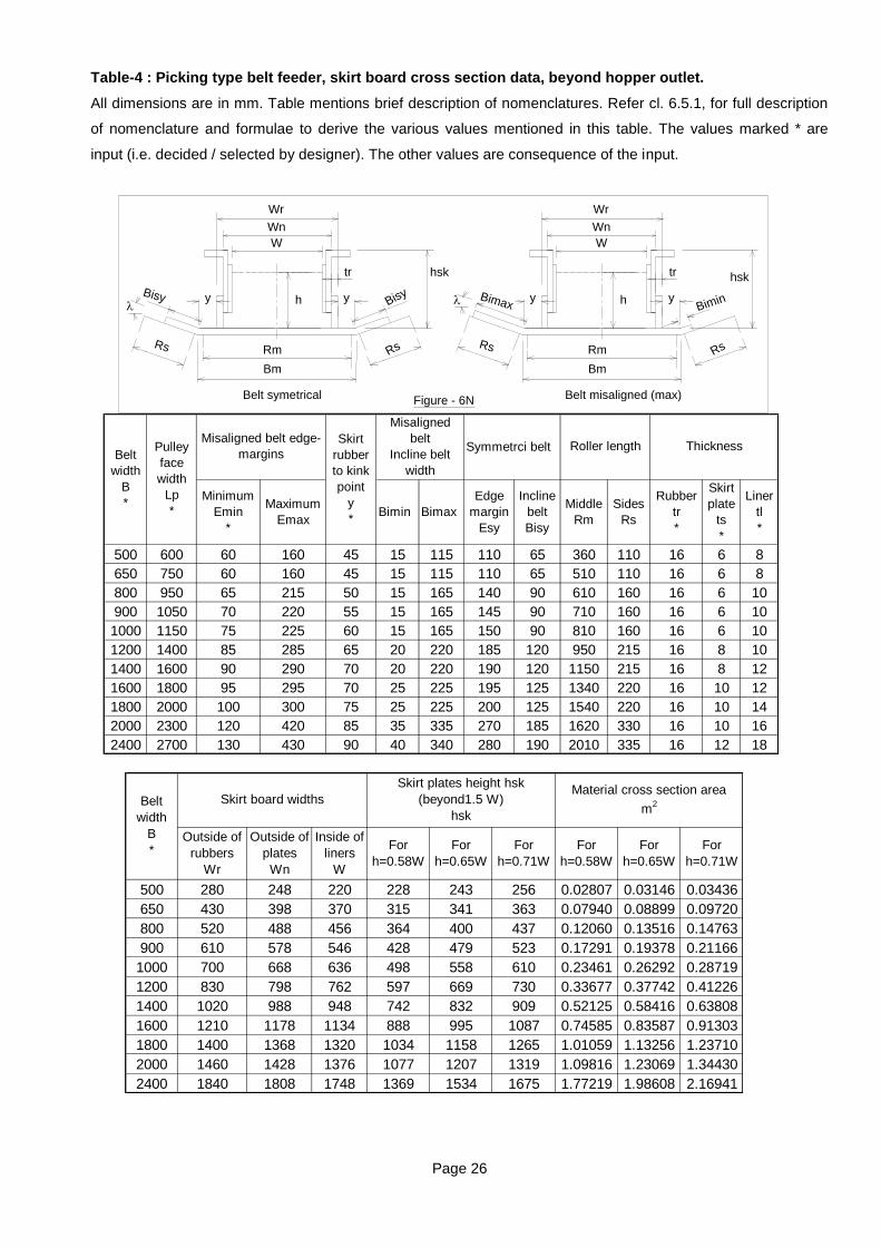
Table-4 : Picking type belt feeder, skirt board cross section data, beyond hopper outlet.
All dimensions are in mm. Table mentions brief description of nomenclatures. Refer cl. 6.5.1, for full description
of nomenclature and formulae to derive the various values mentioned in this table. The values marked * are
input (i.e. decided / selected by designer). The other values are consequence of the input.
W
Belt symetrical
Wn
tr
Wr
hsk
Rm
Bm
Rs
Bisy yy Bisyh
Rs Rs
hBiminy yBimax
Rs
Bm
Rm
hsk
Wr
tr
Wn
W
Belt misaligned (max)
Figure - 6N
Symmetrci belt
Minimum
Emin
*
Maximum
EmaxBimin Bimax
Edge
margin
Esy
Incline
belt
Bisy
Middle
Rm
Sides
Rs
Rubber
tr
*
Skirt
plate
ts
*
Liner
tl
*
500 600 60 160 45 15 115 110 65 360 110 16 6 8
650 750 60 160 45 15 115 110 65 510 110 16 6 8
800 950 65 215 50 15 165 140 90 610 160 16 6 10
900 1050 70 220 55 15 165 145 90 710 160 16 6 10
1000 1150 75 225 60 15 165 150 90 810 160 16 6 10
1200 1400 85 285 65 20 220 185 120 950 215 16 8 10
1400 1600 90 290 70 20 220 190 120 1150 215 16 8 12
1600 1800 95 295 70 25 225 195 125 1340 220 16 10 12
1800 2000 100 300 75 25 225 200 125 1540 220 16 10 14
2000 2300 120 420 85 35 335 270 185 1620 330 16 10 16
2400 2700 130 430 90 40 340 280 190 2010 335 16 12 18
Belt
width
B
*
Pulley
face
width
Lp
*
Skirt
rubber
to kink
point
y
*
Misaligned belt edge-
margins
Misaligned
belt
Incline belt
width
Roller length Thickness
Outside of
rubbers
Wr
Outside of
plates
Wn
Inside of
liners
W
For
h=0.58W
For
h=0.65W
For
h=0.71W
For
h=0.58W
For
h=0.65W
For
h=0.71W
500 280 248 220 228 243 256 0.02807 0.03146 0.03436
650 430 398 370 315 341 363 0.07940 0.08899 0.09720
800 520 488 456 364 400 437 0.12060 0.13516 0.14763
900 610 578 546 428 479 523 0.17291 0.19378 0.21166
1000 700 668 636 498 558 610 0.23461 0.26292 0.28719
1200 830 798 762 597 669 730 0.33677 0.37742 0.41226
1400 1020 988 948 742 832 909 0.52125 0.58416 0.63808
1600 1210 1178 1134 888 995 1087 0.74585 0.83587 0.91303
1800 1400 1368 1320 1034 1158 1265 1.01059 1.13256 1.23710
2000 1460 1428 1376 1077 1207 1319 1.09816 1.23069 1.34430
2400 1840 1808 1748 1369 1534 1675 1.77219 1.98608 2.16941
Skirt plates height hsk
(beyond1.5 W)
hsk
Material cross section area
m2Belt
width
B
*
Skirt board widths

Page 27
Chapter 7: MATERIAL FLOW, HOPPER TO BELT FEEDER
This chapter has 54 pages. Following 8 pages write-up is typical.
MATERIAL FLOW FROM HOPPER TO BELT FEEDER
The hopper outlet is flange connected with skirt board. Thus hopper and skirt board forms continuous enclosed
space for material. The material at hopper outlet is carried away by belt feeder. Thus, belt feeder is continuously
creating cavity in material, at hopper bottom. Hence material in hopper descends down to fill in the cavity being
created by belt feeder. This appears as falling level of material in
hopper. In a continuously operating system; the material so lost in
hopper, is replenished by in-flow system at hopper top. In a
continuously operating system the flow would be balanced each time
(instant), or with respect to time cycle / interval. Figure-7A depicts
schematically the system of in-flow to hopper and out-flow from hopper
to belt feeder. In general, the in-flow system will have comparatively
very high velocity and hence material cross section of very small value.
The hopper material has very large cross section and so very small
velocity. The belt feeder speed is very less compared to in-flow system
and hence its material cross section is large compared in-flow system.
However, in comparison to hopper its flow cross section is quite small
and thereby material velocity in belt feeder is quite large compared to
velocity in hopper zone. In balanced flow system (i.e. without accumulation / loss):
(In-flow system material cross section) x (its velocity) = (Hopper material cross section) x (material velocity in
hopper) = (belt feeder material cross section) x (belt velocity) = (Hopper outlet area) x (Average velocity of
material across outlet).
The foregoing description provides general information about flow velocity, right from in-flow system to belt
feeder. This also considers as if bulk density is constant.
BASIC CONDITION FOR FAIRLY UNIFORM FLOW AT HOPPER OUTLET
The figure-7B shows hopper and belt feeder schematic arrangement. Consider that hopper outlet is divided into
5 equal compartments by imaginary line. The belt segment of Y length (equal to compartment length) is to pick-
Figure-7A
Hopper
Inflowsystem
Belt feeder
5
Y
Figure-7B
A B
4321 V

Page 28
up say 5 tonnes of material from hopper during its travel from A to B. Now bulk material under gravity thrust
create potential for each compartment to put full load of 5 tonne on belt section Y when it comes beneath, i.e.
gravity force will just flood in material without keeping room for next compartment. So, the belt feeder
arrangement needs to be such that when segment Y comes below compartment -1, it will just take / accept
ideally 1 tonne of material in spite of material push. When section-Y reaches to compartment-2, it should take 1
more tonne i.e. here load capacity should be totally 2 tonnes. Likewise at 3rd
compartment, the section-Y
capacity should increase to 3 tonne so that although it is already carrying 2 tonnes, it will take 1 tonne from 3rd
compartment. Ultimately, at 5th compartment it will take 1 more tonne with load carrying capacity of 5 tonne.
Thus, for uniform draw out from hopper outlet, the basic condition is that feeder capacity to draw
material from hopper should increase progressively from inlet end to exit end.
The common and similar (but not identical) example is river, where the river widens in direction of flow so that it
can accept water from downstream
area (figure-7C).
In a screw feeder this requirement
of uniform draw out is achieved by
progressively increasing the screw
diameter, pitch, etc. For the belt
feeder, this condition is fulfilled by
gradually increasing the flow cross
section, from inlet end to outlet end,
so that all zones at hopper outlet
get fairly equal opportunity to add
material into belt feeder
flow. The other
consideration is that the
gradual enlargement of
cross section, reduces the
interference / conflict within
body of material and thereby
improves belt feeder
performance and life.
The belt feeder flow cross
section can be increased by
increasing the skirt board
width (alone) or by
increasing height alone or
by both. However, to
maintain proper flow in
bottom part of hopper, it is
not possible to increase
width and height in isolation.
Tributory river
Main river
Figure-7C
Elevation
Section - AA
A A
Hopper
Feed zone
Feed zone
Skirt board
Skirt board
Figure-7D
Page 29
Both increases simultaneously as explained in chapter-8 cl.-8.14.5. Thus figure-7D shows increase of both to
achieve gradual increase of flow cross section.
It is observed that belt feeder performance would be better with combined increase of skirt board width as well
as height in specific manner. The increasing height of skirt board, apart from increasing capacity, it tends to
reduce shear resistance, and creates material ejecting force. The increasing width also increases the capacity.
Additionally it provides material pushing reaction, and would result into less difficulty in pulling out the material.
The situation is similar to pulling out the wedge from surrounding grip. If the belt feeder is handling granular
material; the gradients on height as well as width can be chosen somewhat freely. However, if the material
happens to be lumpy, the flow area at inlet end cannot be made very small, particularly the width. The lump has
freedom in vertical plane, as there is continuous entity of material and vertically the physical barrier is somewhat
flexible. However, lumps have physical barrier width wise (skirt plates) and lumps jamming can damage the belt.
So, the minimum height at rear end could be around 1.75 times lump size and the minimum width at rear end
could be as per chapter-8 cl.-8.17.0.
The skirt board maximum allowable width (at exit end) is fixed in accordance with belt width (refer chapter-6,
tables-4, 5 and 6). So, one can use this (or somewhat lesser) width at exit end.
As for the skirt plate height at exit end, constructionally there is freedom to choose the height. However, the
general practice suggests that it should not be more than net width of skirt board. This height at exit end would
be in the range of 0.75 to 1.0 times the net width of skirt board. The designer can use mid-way value 0.875, and
review it on analysing the general shear plane (refer page - 81, and also clause - 9.8.0, 9.9.0 and 8.16.0).
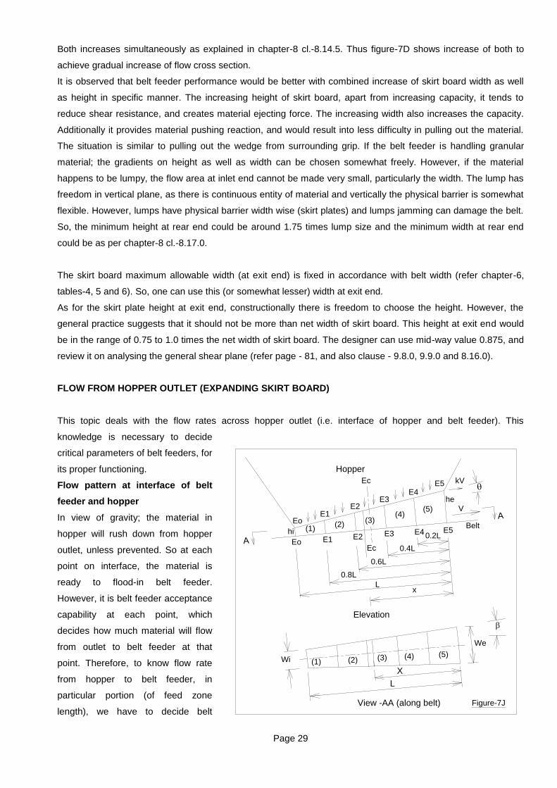
FLOW FROM HOPPER OUTLET (EXPANDING SKIRT BOARD)
This topic deals with the flow rates across hopper outlet (i.e. interface of hopper and belt feeder). This
knowledge is necessary to decide
critical parameters of belt feeders, for
its proper functioning.
Flow pattern at interface of belt
feeder and hopper
In view of gravity; the material in
hopper will rush down from hopper
outlet, unless prevented. So at each
point on interface, the material is
ready to flood-in belt feeder.
However, it is belt feeder acceptance
capability at each point, which
decides how much material will flow
from outlet to belt feeder at that
point. Therefore, to know flow rate
from hopper to belt feeder, in
particular portion (of feed zone
length), we have to decide belt
A
A
Belt
Eo
Eo
E1 E2 E3 E4 E5
E3E2
E1
E4E5
(1)(2)
(3)(4)
(5)
0.2L
0.4L
0.6L
0.8L
Lx
(1) (2) (3) (4) (5)
L
We
Wi
V
kV
hi
he
Elevation
View -AA (along belt) Figure-7J
Hopper
Ec
Ec
X

Page 30
feeder flow rates across vertical planes at entry point and exit point of this portion. The difference between these
two flow rates of belt feeder, is the material flow rate across horizontal plane from hopper into belt feeder, in this
portion.
For the first compartment, no material is entering from tail end side i.e. in-flow at EoEo is zero. Hence for first
compartment, the belt feeder flow rate at E1E1 is also the input in to belt feeder from compartment-1.
Flow rate across interface, into compartment-1 = Flow rate across E1E1 - zero = Flow across E1E1
Flow rate across interface, into compartment-2 = Flow rate across E2E2 - Flow rate across E1E1
Flow rate across interface, into compartment-3 = Flow rate across E3E3 - Flow rate across E2E2
Flow rate across interface, into compartment-4 = Flow rate across E4E4 - Flow rate across E3E3
Flow rate across interface, into compartment-5 = Flow rate across E5E5 - Flow rate across E4E4
Total inflow in 5 compartments of belt feeder = sum of above
Using the equation for flow at E1E1, E2E2, E3E3, E4E4 and E5E5, the flow into belt feeder from interface of
each imaginary compartment, can be derived as mentioned above.
Example-2
Calculate flow pattern from hopper outlet to belt feeder (i.e. across interface); for following data for 1600mm flat
belt feeder, having material shear at interface.
We = 1.124 m, Wi = 0.563 m, he = 0.89 We = 1.0 m
Hi = 0.23 m, L = 5.5 m, V = 0.3 mps, K = 0.555
Also calculate the flow magnitudes for feed zone portion on left side of center line, and for feed zone portion on
right side of center line. The left side is towards rear end and right side is towards head end.
Solution
The calculations are considering 5 compartments of feed zone length.
Ge = (he - hi) L = (1.0 - 0.23) 5.5 = 0.14
Gp = (We - Wi) 2 . L = (1.124 - 0.563) (2 x 5.5) = 0.051
Lz = he Ge = 1.0 0.14 = 7.142857143
2 . Lz = 14.28571429
Flow rate across section E1E1
= (he - 0.8 . L . Ge) . (We - 1.6 . L . Gp) [Lz . (1 + K) + 0.8 . L . (1 - K)] . V 2 . Lz
= (1.0 - 0.8 x 5.5 x 0.14) . (1.124 - 1.6 x 5.5 x 0.051) [7.142857143 x (1 + 0.555) + 0.8 x 5.5 x (1 - 0.555)] x 0.3
14.28571429
= 0.071137257 m3/sec
= 256.1 m3/hr
Flow rate across section E2E2
= (1.0 – 0.6 x 5.5 x 0.14) x (1.124 – 1.2 x 5.5 x 0.051) x [7.142857 x (1.555) + 0.6 x 5.5 x (0.445)] x 0.3
14.285714
= 0.1118735 m3/sec
= 402.74 m3/hr
Flow rate across section E3E3

Page 31
= (1.0 - 0.4 x 5.5 x 0.14) x (1.124 - 0.8 x 5.5 x 0.051) x [7.142857 x (1.555) + 0.4 x 5.5 x (0.445)] x 0.3
14.285714
= 0.158002 m3/sec
= 568.8 m3/hr
Flow across section E4E4
= (1.0 – 0.2 x 5.5 x 0.14) x (1.124 – 0.4 x 5.5 x 0.051) x [7.142857 x (1.555) + 0.2 x 5.5 x (0.445)] x 0.3
14.285714
= 0.208457 m3/sec
= 750.44 m3/hr
Flow across section E5E5
= he . We . (1 + K) . V 2
= 1.0 x 1.124 x (1 + 0.555) x 0.3 2
= 0.262173 m3/sec
= 943.8228 m3/hr
Using the above values of flow across E1E1, E2E2, E3E3, E4E4 and E5E5, the flow into compartment-1,
compartment-2, compartment-3, compartmet-4 and compartment-5, counting from rear end is as below :
Flow into compartment-1 of belt feeder = Flow across E1E1 - zero = 256.1 m3/hr
Flow into compartment-2 of belt feeder = Flow across E2E2 - Flow across E1E1 = 402.74 - 256.1 = 146.64
m3/hr
Flow into compartment-3 of belt feeder = Flow across E3E3 - Flow across E2E2 = 568.8 - 402.74 = 166.06
m3/hr
Flow into compartment-4 of belt feeder = Flow across E4E4 - Flow across E3E3 = 750.44 - 568.8 = 181.64
m3/hr
Flow into compartment-5 of belt feeder = Flow across E5E5 - Flow across E4E4 = 943.82 - 750.44 = 193.38
m3/hr
Total inflow in 5 compartments of belt feeder = sum of above = 943.82 m3/hr
The total inflow from all 5 compartments matches to the flow rate across E5E5, which is finally outflow at exit
end.
The inflow values in individual sections are 256.1, 146.64, 166.06, 181.64 and 193.38 m3/hr. It is not possible to
make these values identical, because it would need differing values of and for each section. This is not
practical from construction and other reasons, and exact matching is also not necessary.
Now, calculations are to be done for flow magnitude for feed zone portion, which is on tail side of center line, and
flow magnitude for feed zone portion, which is on head side of center line. Here, center line means center line of
feed zone. This can be done using data for each compartment as below. The flow on tail side (i.e. center line to
rear side) is ZT. The flow on head side (i.e. center line to forward side) is ZH.
ZT = (compartment-1) + (compartment-2) + (half of compartment-3)
= 256.1 + 146.64 + 0.5 x 166.06
= 485.77 m3/hr (This is 51.47% of total).
ZH = (half of compartment-3) + (compartment-4) + (compartment-5)
= 0.5 x 166.06 + 181.64 + 193.38
Page 32
= 458.05 m3/hr (This is 48.53% of total).
Total ZT + ZH = 485.77 + 458.05 = 943.82 m3/hr
This result can be said as an excellent matching of flow, on both sides of center line of feed zone.
In this example, Ge = 0.14 i.e. = 7.96961°, and Gp = 0.051 i.e. = 2.919555°. The reader to note that the
values of and will be in large digits and unusual figures, because they are derivations of pre-decided
dimensions. Referring to chapter-8, cl.8.14.5, the hopper outlet adapter wall angle would be 20.016° from
vertical (i.e. 70° to horizontal), according to these values of Ge and Gp and formula given in the said clause.
As would be seen from this numerical example, it is not possible to have exactly equal flow from each
compartment. The exactly equal flow will need differing values of or or both, for each compartment. This is
not practical from feeder construction point of view. So, the designer is to see that at least there is reasonable
balance of in-flow into feeder, for first half of feed zone and second half of feed zone.
Some imbalance between them is not directly harmful to belt feeder but would result in to imbalance in hopper
emptying process, and material top face would be at lower level where there is greater flow at underneath outlet
portion. The material top face would be at higher level where the flow is less at underneath outlet portion. This
implies that material in hopper is not descending vertically down, but it is also simultaneously shifting horizontally
at a very slow rate, towards the outlet section, which is emptying fast. Such imbalance is more of concern for tall
hoppers (bin / silo / bunker), if the same results into undesirable flow pattern in hopper. In general, lesser value
of and would tend to increase flow in the rear zone. The more value of and i.e. higher values of taper
(rapidly expanding cross section) will tend to put more material into forward zone. This statement will help the
designer in manipulating the values of and to achieve approximate balance of flow.
Ready to use tables
The book includes ready to use flow balancing tables (17 pages). These tables enables designer to select the
skir-board expansion features close to requirement, and thereby the subsequent design work becomes easy and
quick.
Enclosed two pages show the typical tables.

Page 33
ZT% : Percentage of flow at interface, for feed zone half length, toward tail side.
Analysis basis: Flat belt feeder. The values are fairly applicable to picking type and 3-equal roll belt feeders. The
values are % of total flow, for feed zone half length from tail side to feed zone center line.
The values are ZH % = 100 - ZT%. L is feed zone length (not feeder length).
Wi minimum = 0.25 We. hi minimum = 0.15 m.
The indicated values are ZT%
Belt : 1200 mm L : 4.80 m K = Belt : 1200 mm L : 6.50 m K =
We : 0.762 m he = 0.875 x We = 0.667 m 0.17 We : 0.762 m he = 0.875 x We = 0.667 m 0.17
619 mm 477 mm 334 mm 190 mm 619 mm 476 mm 333 mm 190 mm
1.4926 542 1.1041 542
2.9852 417 2.2081 416
4.4779 291 3.3122 291
5.9705 165 4.4162 165
Belt : 1200 mm L : 1.50 m K = 0.5 Belt : 1200 mm L : 2.00 m K = 0.5
We : 0.762 m he = We = 0.762 m 0.17 We : 0.762 m he = We = 0.762 m 0.17
621 mm 479 mm 336 mm 191 mm 620 mm 478 mm 335 mm 191 mm
5.4256 620 4.1551 617
10.8513 474 8.3102 470
16.2769 324 12.4653 320
21.7026 165 16.6204 165
Belt : 1200 mm L : 2.70 m K = 0.5 Belt : 1200 mm L : 3.60 m K = 0.5
We : 0.762 m he = We = 0.762 m 0.17 We : 0.762 m he = We = 0.762 m 0.17
620 mm 477 mm 334 mm 191 mm 619 mm 477 mm 334 mm 191 mm
3.1170 615 2.3540 614
6.2341 467 4.7079 466
9.3511 317 7.0619 316
12.4681 165 9.4159 165
Belt : 1200 mm L : 4.80 m K = 0.5 Belt : 1200 mm L : 6.50 m K = 0.5
We : 0.762 m he = We = 0.762 m 0.17 We : 0.762 m he = We = 0.762 m 0.17
619 mm 477 mm 334 mm 190 mm 619 mm 476 mm 333 mm 190 mm
1.7724 613 1.3119 613
3.5449 465 2.6238 464
5.3173 315 3.9358 315
7.0898 165 5.2477 165 62.33 55.88 49.43 42.98
70.30 63.03 55.76 48.48
77.67 69.64 61.60 53.56
84.44 75.71 66.97 58.23
degrees
hi
mm
degrees and Wi mm
0.6293 1.2586 1.8879 2.5172
62.33 55.89 49.44 42.98
70.33 63.06 55.78 48.50
77.70 69.66 61.63 53.58
84.46 75.73 66.99 58.24
degrees
hi
mm
degrees and Wi mm
0.8517 1.7034 2.5552 3.4069
62.33 55.90 49.45 42.98
70.37 63.10 55.82 48.52
77.74 69.71 61.67 53.61
84.49 75.76 67.02 58.26
degrees
hi
mm
degrees and Wi mm
1.1346 2.2692 3.4038 4.5383
62.34 55.91 49.46 42.98
70.45 63.18 55.89 48.57
77.83 69.80 61.74 53.66
84.55 75.82 67.07 58.29
degrees
hi
mm
degrees and Wi mm
1.5103 3.0207 4.5310 6.0413
62.36 55.94 49.49 42.98
70.60 63.33 56.02 48.66
77.98 69.95 61.88 53.75
84.65 75.93 67.17 58.34
degrees
hi
mm
degrees and Wi mm
2.0328 4.0656 6.0983 8.1311
62.39 55.99 49.53 42.98
70.85 63.58 56.24 48.81
78.24 70.21 62.11 53.90
84.81 76.11 67.32 58.42
degrees
hi
mm
degrees and Wi mm
2.6964 5.3928 8.0892 10.7856
62.48 56.02 49.56 43.09
70.21 62.95 55.69 48.42
77.48 69.46 61.45 53.43
84.28 75.56 66.85 58.12
0.5625
degrees
hi
mm
degrees and Wi mm
0.6293 1.2586 1.8879 2.5172
62.48 56.03 49.56 43.09
70.23 62.97 55.71 48.43
77.50 69.49 61.47 53.44
84.29 75.58 66.86 58.13
0.5625
degrees
hi
mm
degrees and Wi mm
0.8517 1.7034 2.5552 3.4069
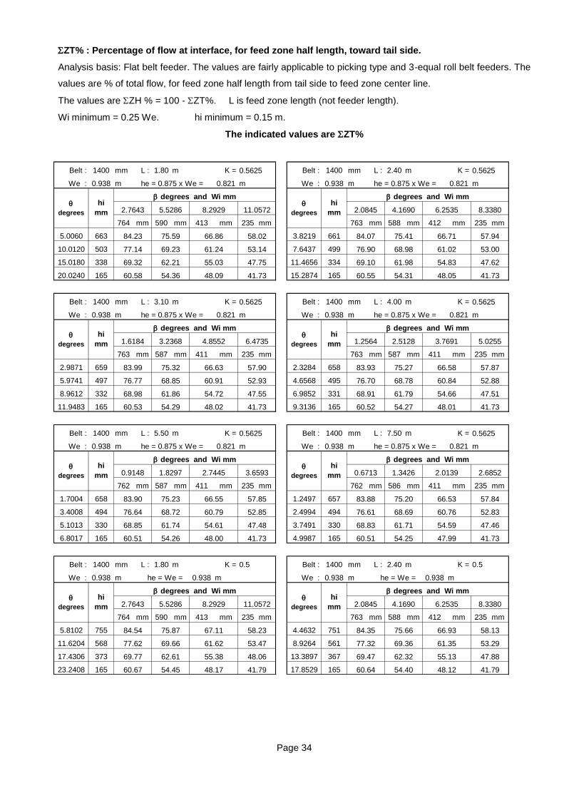
Page 34
ZT% : Percentage of flow at interface, for feed zone half length, toward tail side.
Analysis basis: Flat belt feeder. The values are fairly applicable to picking type and 3-equal roll belt feeders. The
values are % of total flow, for feed zone half length from tail side to feed zone center line.
The values are ZH % = 100 - ZT%. L is feed zone length (not feeder length).
Wi minimum = 0.25 We. hi minimum = 0.15 m.
The indicated values are ZT%
Belt : 1400 mm L : 1.80 m K = Belt : 1400 mm L : 2.40 m K =
We : 0.938 m he = 0.875 x We = 0.821 m 0.17 We : 0.938 m he = 0.875 x We = 0.821 m 0.17
764 mm 590 mm 413 mm 235 mm 763 mm 588 mm 412 mm 235 mm
5.0060 663 3.8219 661
10.0120 503 7.6437 499
15.0180 338 11.4656 334
20.0240 165 15.2874 165
Belt : 1400 mm L : 3.10 m K = Belt : 1400 mm L : 4.00 m K =
We : 0.938 m he = 0.875 x We = 0.821 m 0.17 We : 0.938 m he = 0.875 x We = 0.821 m 0.17
763 mm 587 mm 411 mm 235 mm 763 mm 587 mm 411 mm 235 mm
2.9871 659 2.3284 658
5.9741 497 4.6568 495
8.9612 332 6.9852 331
11.9483 165 9.3136 165
Belt : 1400 mm L : 5.50 m K = Belt : 1400 mm L : 7.50 m K =
We : 0.938 m he = 0.875 x We = 0.821 m 0.17 We : 0.938 m he = 0.875 x We = 0.821 m 0.17
762 mm 587 mm 411 mm 235 mm 762 mm 586 mm 411 mm 235 mm
1.7004 658 1.2497 657
3.4008 494 2.4994 494
5.1013 330 3.7491 330
6.8017 165 4.9987 165
Belt : 1400 mm L : 1.80 m K = 0.5 Belt : 1400 mm L : 2.40 m K = 0.5
We : 0.938 m he = We = 0.938 m 0.17 We : 0.938 m he = We = 0.938 m 0.17
764 mm 590 mm 413 mm 235 mm 763 mm 588 mm 412 mm 235 mm
5.8102 755 4.4632 751
11.6204 568 8.9264 561
17.4306 373 13.3897 367
23.2408 165 17.8529 165 60.64 54.40 48.12 41.79
69.47 62.32 55.13 47.88
77.32 69.36 61.35 53.29
84.35 75.66 66.93 58.13
degrees
hi
mm
degrees and Wi mm
2.0845 4.1690 6.2535 8.3380
60.67 54.45 48.17 41.79
69.77 62.61 55.38 48.06
77.62 69.66 61.62 53.47
84.54 75.87 67.11 58.23
degrees
hi
mm
degrees and Wi mm
2.7643 5.5286 8.2929 11.0572
60.51 54.25 47.99 41.73
68.83 61.71 54.59 47.46
76.61 68.69 60.76 52.83
83.88 75.20 66.53 57.84
0.5625
degrees
hi
mm
degrees and Wi mm
0.6713 1.3426 2.0139 2.6852
60.51 54.26 48.00 41.73
68.85 61.74 54.61 47.48
76.64 68.72 60.79 52.85
83.90 75.23 66.55 57.85
0.5625
degrees
hi
mm
degrees and Wi mm
0.9148 1.8297 2.7445 3.6593
60.52 54.27 48.01 41.73
68.91 61.79 54.66 47.51
76.70 68.78 60.84 52.88
83.93 75.27 66.58 57.87
0.5625
degrees
hi
mm
degrees and Wi mm
1.2564 2.5128 3.7691 5.0255
60.53 54.29 48.02 41.73
68.98 61.86 54.72 47.55
76.77 68.85 60.91 52.93
83.99 75.32 66.63 57.90
0.5625
degrees
hi
mm
degrees and Wi mm
1.6184 3.2368 4.8552 6.4735
60.55 54.31 48.05 41.73
69.10 61.98 54.83 47.62
76.90 68.98 61.02 53.00
84.07 75.41 66.71 57.94
0.5625
degrees
hi
mm
degrees and Wi mm
2.0845 4.1690 6.2535 8.3380
60.58 54.36 48.09 41.73
69.32 62.21 55.03 47.75
77.14 69.23 61.24 53.14
84.23 75.59 66.86 58.02
0.5625
degrees
hi
mm
degrees and Wi mm
2.7643 5.5286 8.2929 11.0572
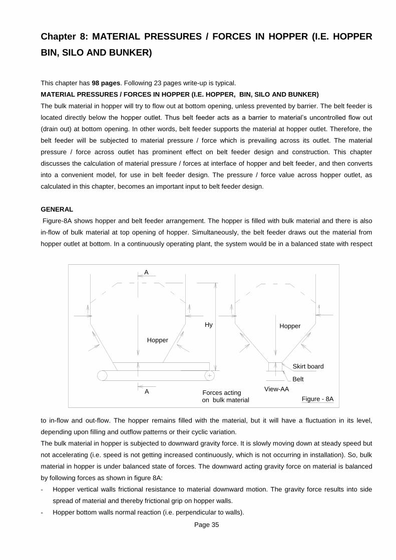
Page 35
Chapter 8: MATERIAL PRESSURES / FORCES IN HOPPER (I.E. HOPPER
BIN, SILO AND BUNKER)
This chapter has 98 pages. Following 23 pages write-up is typical.
MATERIAL PRESSURES / FORCES IN HOPPER (I.E. HOPPER, BIN, SILO AND BUNKER)
The bulk material in hopper will try to flow out at bottom opening, unless prevented by barrier. The belt feeder is
located directly below the hopper outlet. Thus belt feeder acts as a barrier to material‟s uncontrolled flow out
(drain out) at bottom opening. In other words, belt feeder supports the material at hopper outlet. Therefore, the
belt feeder will be subjected to material pressure / force which is prevailing across its outlet. The material
pressure / force across outlet has prominent effect on belt feeder design and construction. This chapter
discusses the calculation of material pressure / forces at interface of hopper and belt feeder, and then converts
into a convenient model, for use in belt feeder design. The pressure / force value across hopper outlet, as
calculated in this chapter, becomes an important input to belt feeder design.
GENERAL
Figure-8A shows hopper and belt feeder arrangement. The hopper is filled with bulk material and there is also
in-flow of bulk material at top opening of hopper. Simultaneously, the belt feeder draws out the material from
hopper outlet at bottom. In a continuously operating plant, the system would be in a balanced state with respect
to in-flow and out-flow. The hopper remains filled with the material, but it will have a fluctuation in its level,
depending upon filling and outflow patterns or their cyclic variation.
The bulk material in hopper is subjected to downward gravity force. It is slowly moving down at steady speed but
not accelerating (i.e. speed is not getting increased continuously, which is not occurring in installation). So, bulk
material in hopper is under balanced state of forces. The downward acting gravity force on material is balanced
by following forces as shown in figure 8A:
- Hopper vertical walls frictional resistance to material downward motion. The gravity force results into side
spread of material and thereby frictional grip on hopper walls.
- Hopper bottom walls normal reaction (i.e. perpendicular to walls).
on bulk materialForces acting
Belt
Hy
Figure - 8A
Hopper
Hopper
Skirt board
A
A
View-AA

Page 36
- Hopper bottom walls frictional resistance acting against material downward motion.
- The belt feeder vertical reaction.
The vertical components of all the forces
adds to zero (vector sum), because, material
is in a state of balance i.e. gravity downward
force is balanced by upward components of
all the earlier mentioned forces (frictions and
reactions).
The next issue is the magnitude of material
weight portion, which is pressing on belt
feeder. Referring to figure-8B, if it would have
been liquid, the pressure at belt level would
have been just .g.Hy and the force would be
this pressure multiplied by liquid (material)
support area of belt feeder. This is so,
because liquid repose angle is zero and it
does not offer shear resistance (in context of
negligible slide velocity applicable to this case). The material column Hy is not subjected to any shear / frictional
resistance by material (liquid) surrounding this column, and hence pressure according to its full height Hy acts at
bottom. In case of material, the downward motion (tendency of motion), relative to surrounding material, is
opposed by the shear / frictional resistance of material surrounding this column. So the pressure value at bottom
is less compared to the liquid.
Thus it is evident that the entire weight of material column from bottom to top, is not resting on belt feeder. In
fact, the major portion of this material column weight, when it tries to move down, is getting transferred to
surrounding material. Hence in this very simplistic analysis, the pressure (weight force) at hopper outlet would be
quite less compared to weight of full column.
The issue of less pressure (force) at hopper outlet, can also be understood by simplistic approach to arching
characteristic of material. As everyone knows from day to day experience, the bulk material has arching
characteristic / ability. In view of this, when material is removed from a portion close to the bottom support, the
entire material does not fall down or flow out like liquid, but tends to form cave due to arching.
This book and chapter is concerned with the material pressure across hopper outlet, which imposes forces on
belt feeder. Now, pressure across hopper outlet depends upon pressure values in hopper at various points. In
fact, outlet pressure is consequence of pressure values from material top face to bottom outlet. Therefore, the
chapter does provide the basic information to enable the calculation of pressure at relevant points in hopper.
However, it is not necessary to entail the hopper elaborate design entire procedure onto belt feeder design.
Hence, this chapter presents calculation procedure for the material forces across hopper outlet, in a manner
relevant to belt feeder, avoiding material testing etc. required for more exact results. This is befitting to the need
of belt feeder. The literature on hopper (bin / bunker / silo) design generally concerns with hopper (silo / bin) of
great height. But more number of belt feeders are used for installations where hopper height is quite less, and
this aspect needs to be given due importance while formulating general approach to belt feeder design, so that
unnecessary complexities are not imposed, where not warranted.
Belt Figure - 8B
Material as if liquid
Hy
resistance zero
Frictional

Page 37
TECHNICAL UNDERSTANDING OF PRESSURE VALUES
The material pressure values have differing basis / reasons for vertical upper portion and bottom converging
portion. Therefore, these sections have different
formulae for pressure values, as described in this
chapter. Again these pressure values are different when
material is flowing out at bottom outlet; and when
material is not flowing out at bottom outlet. The pressure
situation in hopper has been named as dynamic
pressures, when the material is flowing out at bottom
outlet (this is often called as emptying pressures). The
pressure situation in hopper has been named as static
pressures, when the material is not flowing out at bottom
outlet (this can best be said as no-emptying pressures).
But non-emptying is not convenient and hence, the word
static has been chosen. Now, as the static word has been chosen for this case, the first case is named as
dynamic pressure).
The dynamic (emptying) pressure values are comparatively more definite as compared to static (non-emptying)
pressure values, at outlet. In fact, both values are reasonably predicted values for engineering requirements.
The static (i.e. non-emptying) pressure values signify the maximum values during usual situation. For example in
tall hopper, if material remains static for short duration, then it will have pressure values close to dynamic
situation. It can reach the calculated static pressure values for standstill condition of routine nature. Possibly, it
may not cover dead static situation of abnormal nature. The issue is subjective, and cannot be quantified in
terms of time, as a general rule. However, it appears that the same would depend upon daily temperature
variation and compressibility of particular bulk material.
The filling of material in hopper can occur simultaneous to emptying, or may not occur simultaneously. The
dynamic (emptying) pressure are the same irrespective of filling or not filling, provided the hopper is of sufficient
height. The filling of material in tall hopper is to be always done above intersection level (i.e. hopper should not
be emptied below this level). The filling of material in such hopper, when there is no on-going emptying, will
„possibly‟ bring static pressure values close to calculated pressure values, somewhat quicker. The statement is
for hopper of sufficient height.
Now, as regards converging portion of hopper, the pressure values also depend upon geometric shape of
hopper. Therefore, this chapter includes topics for pressure calculation, for belt feeder needs, for following
situations (total of all cases for vertical portion and bottom converging portion).
- The pressure values for vertical portion. Refer cl. 8.5.0 These values are adequate for dynamic as well as
static situation, in context of belt feeder interface.
- The pressure values for horizontal bottom silo, (i.e. hopper converging portion nearly horizontal, say sides
up to 10° incline to horizontal), static situation. Refer cl. 8.8.1.
- The pressure values for horizontal bottom silo, (i.e. hopper converging portion nearly horizontal, say sides
up to 10° incline to horizontal), dynamic situation. Refer cl. 8.8.2.
- Pressure values for steep converging portion of hopper, dynamic (emptying) situation. Refer cl. 8.9.1.
Figure-8D
Vertical
portion
Sloping
portion
Hopper
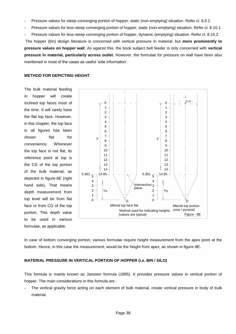
Page 38
- Pressure values for steep converging portion of hopper, static (non-emptying) situation. Refer cl. 8.9.2.
- Pressure values for less-steep converging portion of hopper, static (non-emptying) situation. Refer cl. 8.10.1
- Pressure values for less-steep converging portion of hopper, dynamic (emptying) situation. Refer cl. 8.10.2
The hopper (bin) design literature is concerned with vertical pressure in material, but more prominently to
pressure values on hopper wall. As against this, the book subject belt feeder is only concerned with vertical
pressure in material, particularly across outlet. However, the formulae for pressure on wall have been also
mentioned in most of the cases as useful „side information‟.
METHOD FOR DEPICTING HEIGHT
The bulk material feeding
in hopper will create
inclined top faces most of
the time. It will rarely have
the flat top face. However,
in this chapter, the top face
in all figures has been
shown flat for
convenience. Whenever
the top face is not flat, its
reference point at top is
the CG of the top portion
of the bulk material, as
depicted in figure-8E (right
hand side). That means
depth measurement from
top level will be from flat
face or from CG of the top
portion. This depth value
to be used in various
formulae, as applicable.
In case of bottom converging portion, various formulae require height measurement from the apex point at the
bottom. Hence, in this case the measurement, would be the height from apex, as shown in figure-8E.
MATERIAL PRESSURE IN VERTICAL PORTION OF HOPPER (i.e. BIN / SILO)
This formula is mainly known as Janssen formula (1895). It provides pressure values in vertical portion of
hopper. The main considerations in this formula are :
- The vertical gravity force acting on each element of bulk material, create vertical pressure in body of bulk
material.
14
13
12
11
10
9
8
7
6
5
4
3
2
1
0
Figure - 8E
14.95
O0
5.361
1
2
3
4
5
Yo
y y
Yo
5
4
3
2
1
5.361
0 O
14.95
0
1
2
3
4
5
6
7
8
9
10
11
12
13
14
C.G
Mterial top face flat Mterial top portion cone / pyramid
Intersection plane
(values are typical)
Method used for indicating heights

Page 39
- The vertical pressure creates side pressure (horizontal pressure) due to spreading tendency of bulk material.
This side pressure acts on hopper wall; creating friction grip between hopper wall and bulk material
- The compression or settling or downward motion of bulk material results into situation, whereby upper
portion of bulk material is not able bear fully on lower portion of bulk material. The effect is that the pressure
values increase at diminishing rate, as the depth increases.
Figure-8F shows the material in vertical portion of hopper. Consider a material slice of thickness dy at depth y
from top face. The nomenclature in figure-8F implies following quantities :
y : Depth from top, at the point of analysis, m
: Material usual repose angle, degree
K : Ratio of horizontal and vertical pressure. Here
average value, K = (1 - sin 0.9). Use tested value
when necessary.
Pv : Vertical pressure in bulk material at depth y. This
acts downwards on upper face of slice, N/m2
Pv + dPv : Vertical pressure in bulk material at depth y + dy.
This acts upward on lower face of slice, N/m2
A : Cross section area of slice i.e. cross section area
of hopper (bin). This is uniform for vertical portion.
Janssen formula and this derivation is applicable
to vertical portion only, m2
Pn : Horizontal pressure in bulk material, at depth y.
The hopper (bin) wall applies same pressure on slice, as shown in figure-8F. This is considered as Pn
along slice thickness instead of average of Pn and Pn + dPn. The reason for this is mathematical and
is not the subject here, (like multiplication among increments, etc) N/m2
s : Friction coefficient between hopper wall and slice.
Cr : Circumference of slice edge, m
R : A Cr, which is known as „hydraulic‟ radius, m
: Bulk density, kg/m3. The formula considers this of uniform value, with respect to depth.
The slice is about to slide down (settle down), but is stable in vertical direction (i.e. it is not accelerating in
vertical direction). The „about to slide down‟ situation arises due to compressible nature of underneath material.
During hopper discharge, this slice actually moves downward at slow speed, whereby it is also stable during
hopper emptying. Thus, this formula is applicable to bulk material in hopper, during no out-flow as well as during
out-flow situation (i.e. static and dynamic situation as applicable to installation in running plant).
Now, as the slice is stable in vertical direction; the opposing forces in vertical direction are equal. This provides
following equation.
Pv . A + A . dy . . g = (Pv + dPv) . A + s . Cr . dy . Pn
But, Pn = K . Pv, where K is factor for horizontal pressure
A . Pv + A . . g . dy = A . (Pv + dPv) + s . Cr . K . Pv . dy
The mathematical solution of this equation gives following formula for vertical pressure Pv and horizontal
pressure Pn, at depth y from top.
Pv
Pv + dPv
y
dy
Figure - 8F
s.Pn
PnA. dy
Pns.Pn
Janssen Theory

Page 40
2
R
y.K.sm/N
e
11.
K.s
R.g.Pv
2
R
y.K.sm/N
e
11.
s
R.g.Pv.KPn
The value of R for mostly used shape is as below (partly this is actual and partly this is equivalent applicable).
Circular cross section of diameter d :
4
d
d.
1.
4
d.
Cr
AR
2
:alengthofsidesoftionseccrossSquare
4
a
a.4
a
Cr
AR
2
4
aR:asidealongpressuregcalculatinFor
bthanlessisawhere;bandalengthsside,tionseccrossgulartancRe
)ba(.2
b.aR:bsidealongpressuregcalculatinFor
The value of Pv and Pn can be maximum, when the value of equation in bracket is equal to one. It is obvious
that this can occur when y is infinite. Accordingly,
K.s
R.g.maxPv
s
R.g.
K.s
R.g..KmaxPn
It would be clear from numerical example that Pv becomes nearly maximum at very limited height, and there
after its increase is at insignificant rate.
The factor K in formula is ratio of horizontal pressure divided by vertical pressure. There are differing opinions
about the value of factor K applicable to material situation in hopper (bin), ranging from Rankine factor (active) to
other values. One view is to use Rankine factor (active) for static pressure situation (this will give less horizontal
pressure but more vertical pressure, as if friction is not fully effective). Then, higher value for emptying (dynamic)
condition, which will give less vertical pressure and more horizontal pressure. This book uses the value as
mentioned, i.e. K = 1 - sin i 1 - sin (0.9). Also safety of feeder necessitates vertical pressure somewhat in
upper range and hence, K value as calculated above is not enhanced by factor like 1.1.
s is friction coefficient between hopper wall and material. The author‟s opinion is that it should be either the
said friction coefficient or material internal friction coefficient whichever is less. Because the transfer of holding
force applicable to body of bulk material is finally getting transferred through internal friction grip between
material particles / layers. If the internal friction coefficient is less, then material thin layer (in relation to particle /

Page 41
lump size) in contact with wall will act as imaginary liner, and the body of bulk material will experience friction
resistance according to this imaginary liner.
Example-1 :
Calculate the vertical pressure Pv and horizontal pressure Pn, for vertical portion of hopper, for following
application.
Material : Crushed coal, Bulk density : 800 kg/m3 , Repose angle = 36° (usual repose angle)
Surface friction coefficient s : 0.47 (usual value), basis welded steel flat surface, surface quality somewhat
below average, for calculation here. The designer can also consider it 0.44 as per table-2.
Hopper (bin) cross section : square 5 m x 5 m
Material depth in vertical portion : 15 m (tall height has been chosen to understand pressure variation)
Calculate the value of Pv and Pn at every one meter depth from top face of material. Also calculate the value of
Pv for infinite depth.
Solution :
R = (hopper side length) 4 = 1.25. K = (1 - sin 0.9 ) = [1 - sin (0.9 x 36)] = 0.4642
Pv0 at zero meter depth, Pv0 = 0. Pn0 = K . Pv0 = 0.4642 x 0 = 0 N /m2
Pn1 = K . Pv1 = 0.4642 x 7201 = 3343 N/m2
Pv at 15 meter depth, Pv15 :
Pn15 = K . Pv15 = 0.4642 x 41683 = 19349 N/m2
2
1745392.0
25.1
1x4642.0x47.0
2
R
y.K.s
m/N7201190675.1
11x44964
718.2
11x44964
e
11.
4642.0x47.0
25.1x81.9x8001Pv
m/N
e
11.
K.s
R.g.1Pv
2
2
618088.2
25.1
15x4642.0x47.0
2
R
y.K.s
m/N4168315Pv
m/N33.4168370576.13
11x44964
718.2
11x44964
e
11.
4642.0x47.0
25.1x81.9x80015Pv
m/N
e
11.
K.s
R.g.15Pv

Page 42
The values of Pv and Pn in the range zero to 15 m are as below :
Pv0 = 0 N/m2
Pv1 = 7201 N/m2
Pv2 = 13249 N/m2
Pv3 = 18328 N/m2
Pv4 = 22594 N/m2
Pv5 = 26177 N/m2
Pv6 = 29186 N/m2
Pv7 = 31714 N/m2
Pv8 = 33836 N/m2
Pv9 = 35618 N/m2
Pv10 = 37116 N/m2
Pv11 = 38373 N/m2
Pv12 = 39429 N/m2
Pv13 = 40316 N/m2
Pv14 = 41061 N/m2
Pv15 = 41683 N/m2
Pn0 = 0 N/m2
Pn1 = 3343 N/m2
Pn2 = 6150 N/m2
Pn3 = 8508 N/m2
Pn4 = 10488 N/m2
Pn5 = 12151 N/m2
Pn6 = 13548 N/m2, Pn7 =14721 N/m
2, Pn8 = 15706 N/m
2,
Pn9 = 16533 N/m2, Pn10 =17228 N/m
2, Pn11 = 17812 N/m
2,
Pn12 = 18302 N/m2, Pn13 = 18714 N/m
2, Pn14 = 19059 N/m
2,
Pn15 = 19349 N/m2
Pv max (here, it means hopper depth is infinite), is as below :
The reader to avoid confusion for suffix maximum. As far as this particular hopper is concerned
Pv15 = 41683 N/m2 is its maximum value. However, absolute maximum Pvmax as referred to infinite depth is
44964 N/m2
As can be seen nearly 92.7% of absolute maximum value reaches just at 15 m depth. Only, 7.3% will add into
this if this depth extends to infinite. Figure-8G shows the values of Pv and Pn, as calculated above, at depth
ranging from zero meter to 15 meter.
Figure - 8GD
ep
th in m
0
1
2
3
4
5
6
7
8
9
10
11
12
13
14
15
Pressure N/m2
10000
20000
30000
40000
50000
Graph basis formulae
Pv : vertical pressure
Pn : pressure normal (perpendicular) to wallie horizontal pressure
PvPn
Out-flow (dynamic) or no out-flow (static) Condition
PnPn
Pv
2m/N11.449644642.0x47.0
25.1x81.9x800
K.s
R.g.maxPv

Page 43
PRESSURES IN BULK MATERIAL, STEEP HOPPER
This topic described the pressure values in bulk
material in steep hopper. Refer cl. 8.12.0 for
identification of steep hopper. The dynamic (emptying at
outlet) pressure values are explained in following cl.
8.9.1. The static (non-emptying at outlet) pressure
values are covered in subsequent cl. 8.9.2.
Steep Hopper converging portion, dynamic
pressure
This topic explains the pressure values within the body
of bulk material, in steep converging portion of hopper.
Originally, Walker, Walters, Enstand (and others)
contributed during course of time, for analysis to
calculate pressure values in converging portion of
hopper, just few decades ago.
As explained earlier in cl. 8.6.0 last para, for such steep
hopper; the pressure values in bulk material at outlet
level is also the pressure value applicable on belt
feeder.
Figure-8R shows conical converging portion of steep hopper (bin / silo). The entire body of bulk material is to be
considered as moving downward. Therefore, the material slice shown in this figure moves down vertically. By
large, this motion can be considered of stable nature, for calculation of forces / pressure within the body of bulk
material. The presence of inertial forces, attributed to difference in velocity at intersection level and at outlet
level, is of insignificant value in comparison to other forces / pressure, and hence the same is ignored.
Therefore, magnitude of pressure / forces within body of bulk material is calculated considering the stable /
steady downward motion of this slice. This implies that the sum of downward vertical forces, is equal to the sum
of upward vertical forces. The equation relates to only vertical forces (components) because the slice motion is
in vertical direction.
Nomenclature :
Pv : Vertical pressure in bulk material, general notation, N/m2
Pvi : Vertical pressure in bulk material, at intersection, N/m2
Pn : Pressure perpendicular (normal) to wall, general notation, N/m2
s : Friction coefficient between hopper wall and slice (material). As an average, consider this value 0.9 x
(usual i.e. mean value of friction coefficient) for calculation in „this‟ topic.
s : Surface to material, friction angle, s = tan-1s
i : Material internal effective friction angle. As an average, consider this value same as usual (mean
value) repose angle, for calculation in „this‟ topic. Or when necessary, use tested mean value of internal
effective friction angle + 10%.
: Bulk density, kg/m3. The formula considers this of uniform value, with respect to depth.
s.Pn
Pn
Figure - 8R
Pv + dPv
Pv
Pvi
O
dy
Ho
y
(y or Yo)
Plan

Page 44
Ho : Vertical height from apex to intersection, m
y : Vertical height from apex to slice, m. For convenience in derivation, this is mentioned y. however, in
final result it is renamed as Yo
: Converging portion half angle i.e. angle between hopper side and vertical, degree.
Ke : Ratio of Pn to Pv, during emptying (dynamic) condition i.e. Pn = Ke . Pv
As the y is in increasing order from apex, so depiction of Pv and Pv + dPv is also in ascending order from apex.
Referring figure-8R, the derivation is as below.
Slice bottom face radius = y . tan
Slice top face radius = (y + dy) . tan
Slice average (midpoint) radius = (y + dy 2) . tan
Downward force-1: Due to pressure on slice top.
Force = (y + dy)2 (tan
2 ) . (Pv + dPv)
= (tan2 ) . (y
2 + 2ydy + dy
2) . (Pv + dPv)
= (tan2 ) . (y
2 Pv + 2y dy Pv + dy
2Pv + y
2 dPv + 2ydy dPv + dy
2 dPv
dy2Pv, 2y dy dPv and dy
2 dPv are very small compared to other values and hence same can be ignored in
summation, due to their smaller value compared to others, as per mathematical rule.
Force = (tan2 ) . (y
2 Pv + 2y dy Pv + y
2 dPv)
= (tan2 ) . (y
2 Pv + 2y Pv dy + y
2 dPv)
Downward force-2: Due to slice weight.
Slice weight = (average cross section) x (thickness perpendicular to cross section) . . g
Ignoring y dy dy and dy2 . dy 4, in summation of y
2 dy, as per mathematical rule. The slice weight is as below.
Slice weight = . . g . (tan2 ) . y
2 . dy
Upward force-1 : Due to pressure at bottom.
Upward force = (y . tan )2 . Pv = . (tan
2 ) . y
2 . Pv
Upward force-2 : Due to normal reaction from wall.
Slice average (midpoint) radius = (y + dy 2) . tan
22
tan.2
dyy.tionseccrossaverageSlice
tan.2
dyyradiusaverageSlice
dy4
dydydyydyy.)(tan.g..
dy4
dydyyy.)(tan.g..
g..dy2
dyy.)(tan.weightSlice
222
222
22

Page 45
Slice perimeter = 2 . (y + dy 2) . tan
Slice inclined face length = dy cos
= 2 (tan2) . Pn . y . dy
But Pn = Ke . Pv. Therefore, normal force vertical component = 2 (tan2) . Ke. Pv . y . dy
Upward force-3 due to wall friction.
Equating downward forces sum to upward forces sum
(tan2 ) . (y
2 Pv + 2y Pv dy + y
2 dPv) + . . g . (tan
2 ) . y
2 . dy = . (tan
2 ) . y
2 . Pv + 2 (tan
2) . Ke.
Pv . y . dy + s . 2 . (tan ) . Ke . Pv . y . dy
Dividing both the sides by . (tan2 )
y2 Pv + 2y Pv dy + y
2 dPv + . g . y
2 . dy = y
2 . Pv + 2 . Ke. Pv . y . dy + s . 2 . Ke . Pv . y . dy (tan )
2y Pv dy + y2 dPv + . g . y
2 . dy = 2 . Ke. Pv . y . dy + s . 2 . Ke . Pv . y . dy tan
y2 dPv = 2 . Ke. Pv . y . dy + [(s . 2 . Ke . Pv . y . dy) (tan )] - 2y Pv dy - . g . y
2 . dy
Dividing both the sides by y2 dy
Pn.2
dydyy)(tan2
sin.Pn.cos
dy.)(tan.
2
dyy2componentverticalforceNormal
Pn.cos
dy.)(tan.
2
dyy2forceNormal
cos
dy.)(tan.
2
dyy2wallwithareacontactSlice
22
dyy.Pv.Ke.)(tan.2.s
Pv.Ke.2
dydyy)(tan.2.s
Pn.dy.)(tan.2
dyy2.s
cos.Pn.cos
dy.)(tan.
2
dyy2.scomponentverticalforceFrictional
Pn.cos
dy.)(tan.
2
dyy2.sforceFriction
)beforeas(Pn.cos
dy.)(tan.
2
dyy2forcelNorma
2
g.2Ketan
s.Ke2
y
Pv
dy
dPv
g.2tan
Ke.2.sKe.2
y
Pv
dy
dPv
g.y
Pv.2
tan.y
Pv.Ke.2.s
y
Pv.Ke.2
dy
dPv

Page 46
)napplicatiospecificforttanconsisNwhere(2Ketan
s.Ke2NIf
g.y
PvN
dy
dPv
This equation is a linear differential equation of first order and first degree. Therefore, its solution is derived by
integrating factor (IF) method. The solution results into following equation.
One can use any one of the above equation to calculate Pv. However, its more convenient (easy to remember)
form is as below :
As y is measured from apex -O, it is named Yo to distinguish it from y used to measure depth from top.
Therefore, equation is as below , where y = Yo
In equation for N, the multiplier 2 to bracketed value is related to shape i.e. shape factor. It is 2 for cone or
pyramid shaped hopper, but its value is different for rectangular shape hopper. Replacing this „2‟ by shape factor
Cs, the equation for N is as below :
Where Cs = 2 for circular or square cross section of hopper, as derived in this topic.
Cs = (1 + a b) for rectangular cross section of hopper, having width = a and length = b as per norms.
Sometimes hopper top (intersection) cross section is square, but bottom outlet is rectangle. In this case, the
engineering approximation can be to use Cs value as an average of square and rectangle.
NN
Ho
YoPvi
Ho
Yo
Ho
Yo.
1N
Ho.g.Pv
2Ketan
s.KeCsN
NN
N
N
N
N
N
N
Ho
y.Pvi
Ho
y
Ho
y.
1N
Ho.g.
Ho
y.Pvi
Ho.1N
y.Ho.g.
Ho
Ho
1N
y.g.
Ho
y.Pvi
Ho.1N
y.Ho.g.
1N
y.g.Pv
N
N
N
N
N
N
N
NN
Ho
y.Pvi
Ho.1N
y.Ho.g.
1N
y.g.
Ho.1N
Ho.g..y
Ho
Pvi.y
1N
y.g.
Ho
1N
Ho.g.Pvi
y1N
y.g.Pv
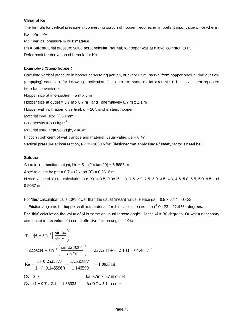
Page 47
Value of Ke
The formula for vertical pressure in converging portion of hopper, requires an important input value of Ke where :
Ke = Pn Pv
Pv = vertical pressure in bulk material
Pn = Bulk material pressure value perpendicular (normal) to hopper wall at a level common to Pv.
Refer book for derivation of formula for Ke.
Example-3 (Steep hopper)
Calculate vertical pressure in hopper converging portion, at every 0.5m interval from hopper apex during out-flow
(emptying) condition, for following application. The data are same as for example-1, but have been repeated
here for convenience.
Hopper size at intersection = 5 m x 5 m
Hopper size at outlet = 0.7 m x 0.7 m and alternatively 0.7 m x 2.1 m
Hopper wall inclination to vertical, = 20°, and is steep hopper.
Material coal, size (-) 50 mm,
Bulk density = 800 kg/m3
Material usual repose angle, = 36°
Friction coefficient of wall surface and material, usual value, s = 0.47
Vertical pressure at intersection, Pvi = 41683 N/m2 (designer can apply surge / safety factor if need be).
Solution
Apex to intersection height, Ho = 5 (2 x tan 20) = 6.8687 m
Apex to outlet height = 0.7 (2 x tan 20) = 0.9616 m
Hence value of Yo for calculation are, Yo = 0.5, 0.9616, 1.0, 1.5, 2.0, 2.5, 3.0, 3.5, 4.0, 4.5, 5.0, 5.5, 6.0, 6.5 and
6.8687 m.
For „this‟ calculation s is 10% lower than the usual (mean) value. Hence s = 0.9 x 0.47 = 0.423
Friction angle s for hopper wall and material, for this calculation s = tan-1
0.423 = 22.9284 degrees.
For „this‟ calculation the value of i is same as usual repose angle. Hence i = 36 degrees. Or when necessary
use tested mean value of internal effective friction angle + 10%.
Cs = 2.0 for 0.7m x 0.7 m outlet.
Cs = (1 + 0.7 2.1) = 1.33333 for 0.7 x 2.1 m outlet.
093318.1146590.1
2535877.1
)146596.0(1
2535877.01Ke
4417.645133.419284.2236sin
9284.22sinsin9284.22
isin
ssinsins
1
1
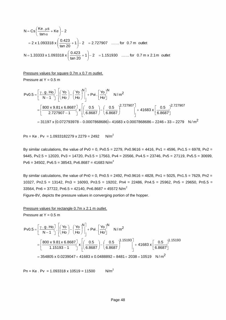
Page 48
Pressure values for square 0.7m x 0.7 m outlet.
Pressure at Y = 0.5 m
Pn = Ke . Pv = 1.0933182279 x 2279 = 2492 N/m2
By similar calculations, the value of Pv0 = 0, Pv0.5 = 2279, Pv0.9616 = 4416, Pv1 = 4596, Pv1.5 = 6978, Pv2 =
9445, Pv2.5 = 12020, Pv3 = 14720, Pv3.5 = 17563, Pv4 = 20566, Pv4.5 = 23746, Pv5 = 27119, Pv5.5 = 30699,
Pv6 = 34502, Pv6.5 = 38543, Pv6.8687 = 41683 N/m2
By similar calculations, the value of Pn0 = 0, Pn0.5 = 2492, Pn0.9616 = 4828, Pn1 = 5025, Pn1.5 = 7629, Pn2 =
10327, Pn2.5 = 13142, Pn3 = 16093, Pn3.5 = 19202, Pn4 = 22486, Pn4.5 = 25962, Pn5 = 29650, Pn5.5 =
33564, Pn6 = 37722, Pn6.5 = 42140, Pn6.8687 = 45572 N/m2
Figure-8V, depicts the pressure values in converging portion of the hopper.
Pressure values for rectangle 0.7m x 2.1 m outlet.
Pressure at Y = 0.5 m
Pn = Ke . Pv = 1.093318 x 10519 = 11500 N/m2
outletm1.2xm7.0for151930.12120tan
423.0x093318.1x33333.1N
outletm7.0for727907.22120tan
423.0x093318.1x2
2Ketan
s.KeCsN
2
727907.2727907.2
2NN
m/N22793322460007868686.0x416830007868686.0072793978.0x31197
8687.6
5.0x41683
8687.6
5.0
8687.6
5.0x
1727907.2
8687.6x81.9x800
m/NHo
Yo.Pvi
Ho
Yo
Ho
Yo.
1N
Ho.g.5.0Pv
2
15193.115193.1
2NN
m/N10519203884810488892.0x416830239047.0x354805
8687.6
5.0x41683
8687.6
5.0
8687.6
5.0x
115193.1
8687.6x81.9x800
m/NHo
Yo.Pvi
Ho
Yo
Ho
Yo.
1N
Ho.g.5.0Pv

Page 49
By similar calculations, the value of Pv0 = 0, Pv0.5 = 10519, Pv0.9616 = 17156, Pv1 = 17639, Pv1.5 = 23217,
Pv2 = 27723, Pv2.5 = 31395, Pv3 = 34379, Pv3.5 = 36775, Pv4 = 38655, Pv4.5 = 40075, Pv5 = 41078, Pv5.5 =
41701, Pv6 = 41973, Pv6.5 = 41919, Pv6.8687 = 41683 N/m2
By similar calculations, the value of Pn0 = 0, Pn0.5 = 11500, Pn0.9616 = 18757, Pn1 = 19286, Pn1.5 = 25383,
Pn2 = 30310, Pn2.5 = 34325, Pn3 = 37588, Pn3.5 = 40207, Pn4 = 42262, Pn4.5 = 43815, Pn5 = 44912, Pn5.5 =
45593, Pn6 = 45890, Pn6.5 = 45830, Pn6.8687 = 45572 N/m2
Figure-8V, depicts the pressure values in converging portion of the hopper. This example is to understand
pressure values and it does not indirectly imply use of belt feeder for the same.
Comments
As could be seen from graph figure-8V, the Pv value at intersection is the same as in vertical portion, but Pn
value generally increases at intersection compared to vertical portion.
The Pv value as well as Pn values diminish as one approaches towards apex. These values are zero at apex.
This continued reduction in pressure towards outlet is attributed to arch stress condition of material in converging
portion. The flow behaviour is such that it maintains this stress condition during outflow as well as during short
time stoppage of outflow (i.e. it will not instantly acquire static pressure values).
The formula analysis indicates that the graph shape can bulge-out or bulge-in depending upon parameters. It
also indicates that the graph shape near outlet (to apex) is nearly straight line. This feature is useful for
equivalent model to decide outlet force (i.e. material force acting on belt feeder, when skirt board width is of
expanding type). This nearly linear shape of graph at outlet results into {material vertical force equivalent column
height} {skirt board width} = constant, which is named as C2.
The material pressure values (particularly Pn) can have fluctuation (surges) due to roughness in hopper wall
surface in vertical portion. Therefore, hopper (bin) design considers the pressure amplification factor on pressure
values calculated as per Janssen formula.
Such pressure surge can arise / vanish during material flow in vertical portion of hopper. The average value can
be taken as 1.25 and could be up to 1.6 where more reliable (safe) design is required for hopper (refer DIN for
contractual needs). However, for pressure values at outlet, which is concern of belt feeder, these surges in Pvi
have partial influence, due to nature of the formula. However, designer can certainly apply this amplification
(surge) factor on Pvi, if he so decides.
Also, reader to note that safety considerations for hopper and belt feeder need not be same. So, designer can
use appropriate value of amplification factor on Pvi, for belt feeder.

Page 50
Example-5 (The data are for explaining calculation and need not imply its use). This is less-steep hopper.
Calculate vertical pressure in hopper converging portion, at every 0.5 m interval from hopper apex during no-
outflow (non-emptying) condition and outflow (emptying) condition, for following application. The data are same
(except wall angle) as for example-4, but have been repeated here for convenience.
Hopper size at intersection = 5 m x 5 m
Hopper size at outlet = 0.7 m x 0.7 m and alternatively 0.7 m x 2.1 m
Hopper wall inclination to vertical, = 40°, and is less-steep.
Material size (-) 50 mm,
Bulk density = 800 kg/m3
Material usual (mean) repose angle, 36°
Friction coefficient, wall surface and material, usual (mean) value 0.47.
Vertical pressure at intersection, Pvi = 41683 N/m2
Solution
For the calculation here, s = 0.9 x 0.47 = 0.423
Static pressure calculation 0.7 m x 0.7 m opening
This is square opening. So, Cs = 2
The apex to intersection height, Ho = 5 (2 x tan 40) = 2.979
1
2
3
4
5
0
Pressure N/m2
50000
40000
30000
20000
10000
Steep hopper
5m x 5m
Pressure in bulk material
Pn : pressure normal (perpendicular) to wall, general notation
Pv : vertical pressure, general notation
Graph basis formulae
'Dynamic' (out flow) Condition
Figure - 8V
A
De
pth
in
m
0.751
5.9071m
Pn PnPv
6.8687m
Pvi
0.9616m
O
6
6.8687
Pv
Pn
Pv
Pn
Outlet square opening-outlet rectangle(1:3) opening-
0.9616
PnPv
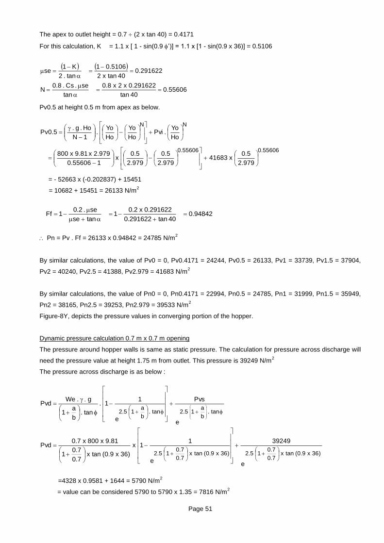
Page 51
The apex to outlet height = 0.7 (2 x tan 40) = 0.4171
For this calculation, K = 1.1 x [ 1 - sin(0.9 ‟)] = 1.1 x [1 - sin(0.9 x 36)] = 0.5106
Pv0.5 at height 0.5 m from apex as below.
= - 52663 x (-0.202837) + 15451
= 10682 + 15451 = 26133 N/m2
Pn = Pv . Ff = 26133 x 0.94842 = 24785 N/m2
By similar calculations, the value of Pv0 = 0, Pv0.4171 = 24244, Pv0.5 = 26133, Pv1 = 33739, Pv1.5 = 37904,
Pv2 = 40240, Pv2.5 = 41388, Pv2.979 = 41683 N/m2
By similar calculations, the value of Pn0 = 0, Pn0.4171 = 22994, Pn0.5 = 24785, Pn1 = 31999, Pn1.5 = 35949,
Pn2 = 38165, Pn2.5 = 39253, Pn2.979 = 39533 N/m2
Figure-8Y, depicts the pressure values in converging portion of the hopper.
Dynamic pressure calculation 0.7 m x 0.7 m opening
The pressure around hopper walls is same as static pressure. The calculation for pressure across discharge will
need the pressure value at height 1.75 m from outlet. This pressure is 39249 N/m2
The pressure across discharge is as below :
=4328 x 0.9581 + 1644 = 5790 N/m2
= value can be considered 5790 to 5790 x 1.35 = 7816 N/m2
55606.040tan
291622.0x2x8.0
tan
se.Cs.8.0N
291622.040tanx2
5106.01
tan.2
K1se
55606.055606.0
NN
979.2
5.0x41683
979.2
5.0
979.2
5.0x
155606.0
979.2x81.9x800
Ho
Yo.Pvi
Ho
Yo
Ho
Yo.
1N
Ho.g.5.0Pv
94842.040tan291622.0
291622.0x2.01
tanse
se.2.01Ff
)36x9.0(tanx7.0
7.015.2)36x9.0(tanx
7.0
7.015.2
tan.b
a15.2tan.
b
a15.2
e
39249
e
11x
)36x9.0(tanx7.0
7.01
81.9x800x7.0Pvd
e
Pvs
e
11.
tan.b
a1
g.WePvd
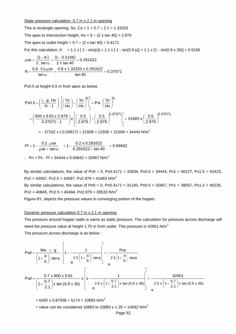
Page 52
Static pressure calculation 0.7 m x 2.1 m opening
This is rectangle opening. So, Cs = 1 + 0.7 2.1 = 1.33333
The apex to intersection height, Ho = 5 (2 x tan 40) = 2.979
The apex to outlet height = 0.7 (2 x tan 40) = 0.4171
For this calculation, K = 1.1 x [ 1 - sin(i)] 1.1 x [ 1 - sin(0.9 )] = 1.1 x [1 - sin(0.9 x 36)] = 0.5106
Pv0.5 at height 0.5 m from apex as below.
= - 37152 x (-0.34817) + 21509 = 12935 + 21509 = 34444 N/m2
Pn = Pv . Ff = 34444 x 0.94842 = 32667 N/m2
By similar calculations, the value of Pv0 = 0, Pv0.4171 = 32834, Pv0.5 = 34444, Pv1 = 40127, Pv1.5 = 42423,
Pv2 = 43067, Pv2.5 = 42697, Pv2.979 = 41683 N/m2
By similar calculations, the value of Pn0 = 0, Pn0.4171 = 31140, Pn0.5 = 32667, Pn1 = 38057, Pn1.5 = 40235,
Pn2 = 40845, Pn2.5 = 40494, Pn2.979 = 39533 N/m2
Figure-8Y, depicts the pressure values in converging portion of the hopper.
Dynamic pressure calculation 0.7 m x 2.1 m opening
The pressure around hopper walls is same as static pressure. The calculation for pressure across discharge will
need the pressure value at height 1.75 m from outlet. This pressure is 42901 N/m2
The pressure across discharge is as below :
= 6492 x 0.87938 + 5174 = 10883 N/m2
= value can be considered 10883 to 10883 x 1.35 = 14692 N/m2
37071.037071.0
NN
979.2
5.0x41683
979.2
5.0
979.2
5.0x
137071.0
979.2x81.9x800
Ho
Yo.Pvi
Ho
Yo
Ho
Yo.
1N
Ho.g.5.0Pv
94842.040tan291622.0
291622.0x2.01
tanse
se.2.01Ff
)36x9.0(tanx1.2
7.01x5.2)36x9.0(tanx
1.2
7.01x5.2
tan.b
a15.2tan.
b
a15.2
e
42901
e
11x
)36x9.0(tanx1.2
7.01
81.9x800x7.0Pvd
e
Pvs
e
11.
tan.b
a1
g.WePvd
37071.040tan
291622.0x33333.1x8.0
tan
seCs.8.0N
291622.040tanx2
5106.01
tan.2
K1se
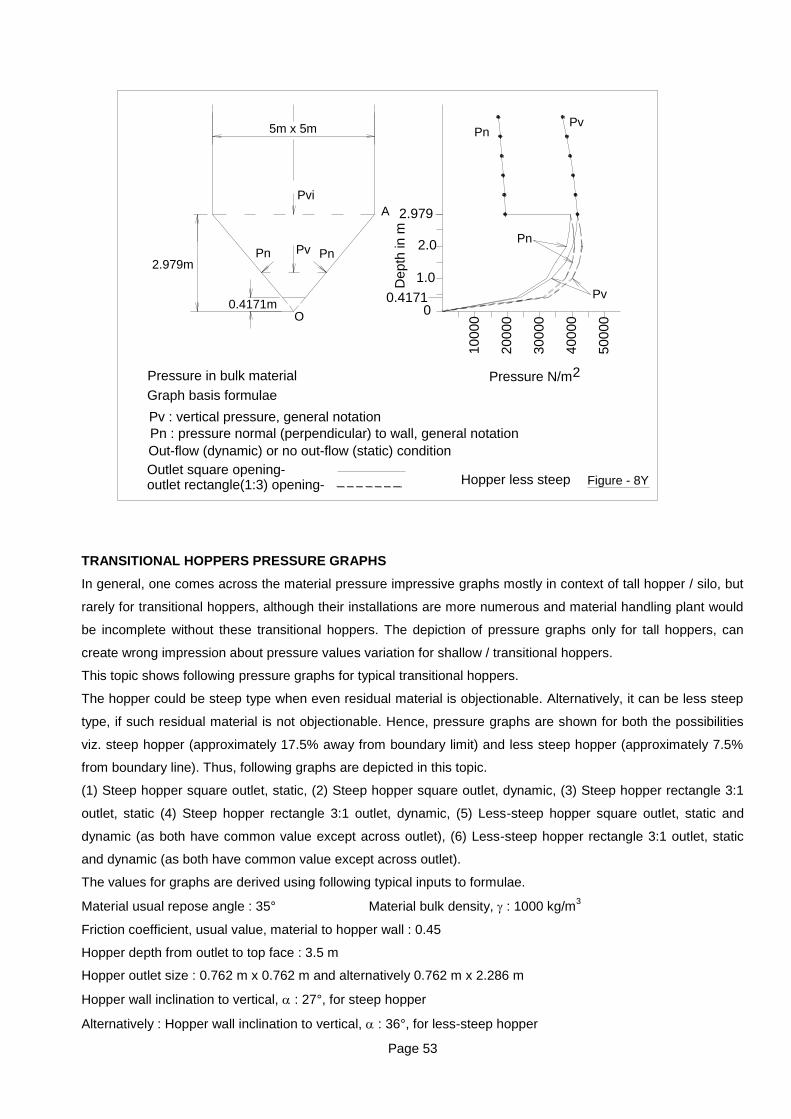
Page 53
TRANSITIONAL HOPPERS PRESSURE GRAPHS
In general, one comes across the material pressure impressive graphs mostly in context of tall hopper / silo, but
rarely for transitional hoppers, although their installations are more numerous and material handling plant would
be incomplete without these transitional hoppers. The depiction of pressure graphs only for tall hoppers, can
create wrong impression about pressure values variation for shallow / transitional hoppers.
This topic shows following pressure graphs for typical transitional hoppers.
The hopper could be steep type when even residual material is objectionable. Alternatively, it can be less steep
type, if such residual material is not objectionable. Hence, pressure graphs are shown for both the possibilities
viz. steep hopper (approximately 17.5% away from boundary limit) and less steep hopper (approximately 7.5%
from boundary line). Thus, following graphs are depicted in this topic.
(1) Steep hopper square outlet, static, (2) Steep hopper square outlet, dynamic, (3) Steep hopper rectangle 3:1
outlet, static (4) Steep hopper rectangle 3:1 outlet, dynamic, (5) Less-steep hopper square outlet, static and
dynamic (as both have common value except across outlet), (6) Less-steep hopper rectangle 3:1 outlet, static
and dynamic (as both have common value except across outlet).
The values for graphs are derived using following typical inputs to formulae.
Material usual repose angle : 35° Material bulk density, : 1000 kg/m3
Friction coefficient, usual value, material to hopper wall : 0.45
Hopper depth from outlet to top face : 3.5 m
Hopper outlet size : 0.762 m x 0.762 m and alternatively 0.762 m x 2.286 m
Hopper wall inclination to vertical, : 27°, for steep hopper
Alternatively : Hopper wall inclination to vertical, : 36°, for less-steep hopper
5m x 5m
Pressure N/m2Pressure in bulk material
Pn : pressure normal (perpendicular) to wall, general notation
Pv : vertical pressure, general notation
Graph basis formulae
Out-flow (dynamic) or no out-flow (static) condition
Figure - 8Y
A
Depth
in m
2.979
50000
40000
30000
20000
10000
Pn PnPv
2.979m
Pvi
0.4171mO
0
Hopper less steep
0.4171
1.0
2.0Pn
Pv
Outlet square opening-outlet rectangle(1:3) opening-
PvPn

Page 54
Figure - 8c
3.455m
0.7477m
0.655m
2.8m3.5477m
0.762m
27°3.455m
0.655m
3.3244m
0.5244m
2.8m
0.762m
36°
Steep hopper Less-steep hopper
27°
0.762m
3.5477m2.8m
0.655m
0.7477m 0
0.50.7477m
1.0
1.5
2.0
2.5
3.0
3.5477
4.2027
50
00
10000
15000
20000
Pv
Steep hopper static pressures
Pn
Pv
Pn
2Pressure N/m
Depth
in m
outlet rectangle(1:3) opening-Outlet square opening-
(No out - flow) Condition
Graph basis formulae
Pv : vertical pressure, general notation
Pn : pressure normal (perpendicular) to wall, general notation
Pressure in bulk material
Figure - 8d
Pn
Pv
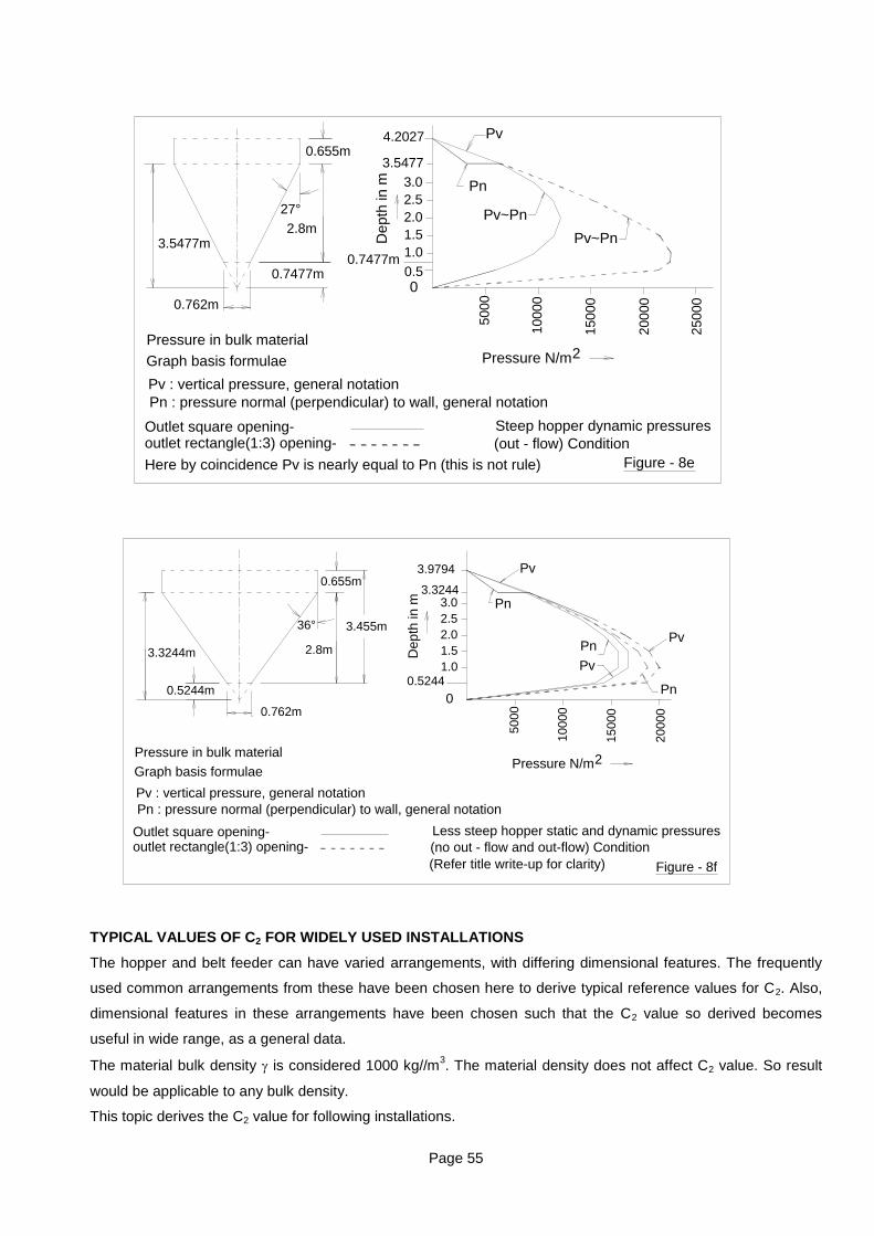
Page 55
TYPICAL VALUES OF C2 FOR WIDELY USED INSTALLATIONS
The hopper and belt feeder can have varied arrangements, with differing dimensional features. The frequently
used common arrangements from these have been chosen here to derive typical reference values for C2. Also,
dimensional features in these arrangements have been chosen such that the C2 value so derived becomes
useful in wide range, as a general data.
The material bulk density is considered 1000 kg//m3. The material density does not affect C2 value. So result
would be applicable to any bulk density.
This topic derives the C2 value for following installations.
Figure - 8e
Pressure in bulk material
Pn : pressure normal (perpendicular) to wall, general notation
Pv : vertical pressure, general notation
Graph basis formulae
(out - flow) ConditionOutlet square opening-outlet rectangle(1:3) opening-
De
pth
in
m
Pressure N/m2
Steep hopper dynamic pressures
20000
15000
10000
5000
4.2027
3.5477
3.0
2.5
2.0
1.5
1.00.7477m
0.5 0
0.7477m
0.655m
2.8m3.5477m
0.762m
27°
25000
Pv~Pn
Pv~Pn
Here by coincidence Pv is nearly equal to Pn (this is not rule)
Pn
Pv
36°
0.762m
2.8m
0.5244m
3.3244m
0.655m
3.455m
Depth
in m
20000
15000
10000
5000
3.9794
3.32443.0
2.5
2.0
1.5
1.0
0
Pressure N/m2
0.5244
Pv
PnPv
Pn
outlet rectangle(1:3) opening-Outlet square opening-
Graph basis formulae
Pv : vertical pressure, general notation
Pn : pressure normal (perpendicular) to wall, general notation
Pressure in bulk material
Less steep hopper static and dynamic pressures
(no out - flow and out-flow) Condition
Figure - 8f(Refer title write-up for clarity)
Pn
Pv

Page 56
1) Reclaim hopper fed by pay-loader. The arrangement comprises of hopper, belt feeder and belt conveyor.
The belt conveyor is at ground level or in trench. The hopper is of less steep type and outlet is square or
rectangle 3:1.
2) Reclaim hopper fed by bulldozers. The arrangement comprises of hopper, belt feeder and belt conveyor.
The belt feeder as well as belt conveyor are in tunnel. The hopper is of steep type or less steep type, and
outlet is square or rectangle 3:1.
3) Unloading hopper for trucks. The belt feeder and conveyor are in tunnel. The hopper is of steep type or less
steep type and outlet is square or rectangle 3:1
4) Tippler installations for unloading of wagons. Wagon capacity upto 80 tonnes. Hopper capacity upto 200 m3
gross. The hopper is of steep type or less steep type and outlet is rectangle 5:1.
5) Tall hopper / silo installations, hopper of steep type or less steep type. The outlet is square or rectangle 3:1.
(Not described here as reader can have idea from example - 3, 4, and 5).
Firstly, the C2 value will depend upon whether the hopper is of steep type or less steep type. So, C2 values are
derived for following hopper types :
- For steep hopper, the used value of is approximately 20% less than boundary line value of for square
outlet. In case of rectangle outlet, the used value is 30% less than boundary line value.
- For less steep hopper, the used value of is approx. 7.5% more than boundary line value of .
The mentioned boundary margins are typical boundary values considered here and do not imply rule. In
application design, the designer can choose the boundary margins as explained in cl.8.12.0 last paragraph-
Summary, best suited to his application.
Secondly, the C2 values are also affected by material flowability (repose angle) and friction coefficient between
material and hopper wall. This can have very large (unlimited) combinations. However, to create ready
reference, C2 values for feel of the subject, following two sets of input parameters have been considered.
- Grain type materials (like barley, wheat, rice, soya bean, castor beans, oat, maze, etc.), which have low
value of repose angle and also the low value of friction coefficient between material and steel wall. This set
of parameters, considers material usual repose angle equal to 26 degree and usual value of friction
coefficient with wall as 0.28 (steel surface without protruding bolt, nuts and edges). This data would provide
feel about C2 value for such application.
- Industrial average materials (like limestone, black coal, broken granite, ores, etc) which have average value
of repose angle 36 degree and usual value of friction coefficient with wall as 0.47 (steel surface without
protruding bolt, nuts and edges). This data would provide feel about C2 value for such application.
The reader to note that above mentioned two sets are for getting general idea about C2 value. It may also be
noted that two materials of same repose angle can have different value of friction coefficients on wall. Therefore,
friction coefficient value is chosen as a mean of average materials. Use C2 value preferably based on specific
data, when dealing with construction design. Thus, we now have following combinations for calculations (steep
hopper, less steep hopper and two sets of material data).
- Grain type material, steep hopper
- Grain type material, less steep hopper
- Industrial average material, steep hopper
- Industrial average material, less steep hopper
The boundary line value of and the chosen value of for above two sets of materials are as below.
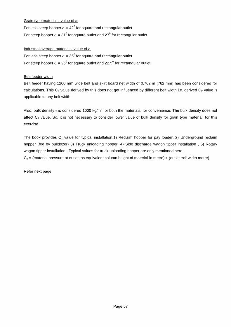
Page 57
Grain type materials, value of
For less steep hopper = 420 for square and rectangular outlet.
For steep hopper = 310 for square outlet and 27
0 for rectangular outlet.
Industrial average materials, value of
For less steep hopper = 360 for square and rectangular outlet.
For steep hopper = 250 for square outlet and 22.5
0 for rectangular outlet.
Belt feeder width
Belt feeder having 1200 mm wide belt and skirt board net width of 0.762 m (762 mm) has been considered for
calculations. This C2 value derived by this does not get influenced by different belt width i.e. derived C2 value is
applicable to any belt width.
Also, bulk density is considered 1000 kg/m3 for both the materials, for convenience. The bulk density does not
affect C2 value. So, it is not necessary to consider lower value of bulk density for grain type material, for this
exercise.
The book provides C2 value for typical installation.1) Reclaim hopper for pay loader, 2) Underground reclaim
hopper (fed by bulldozer) 3) Truck unloading hopper, 4) Side discharge wagon tipper installation , 5) Rotary
wagon tipper installation. Typical values for truck unloading hopper are only mentioned here.
C2 = (material pressure at outlet, as equivalent column height of material in metre) (outlet exit width metre)
Refer next page
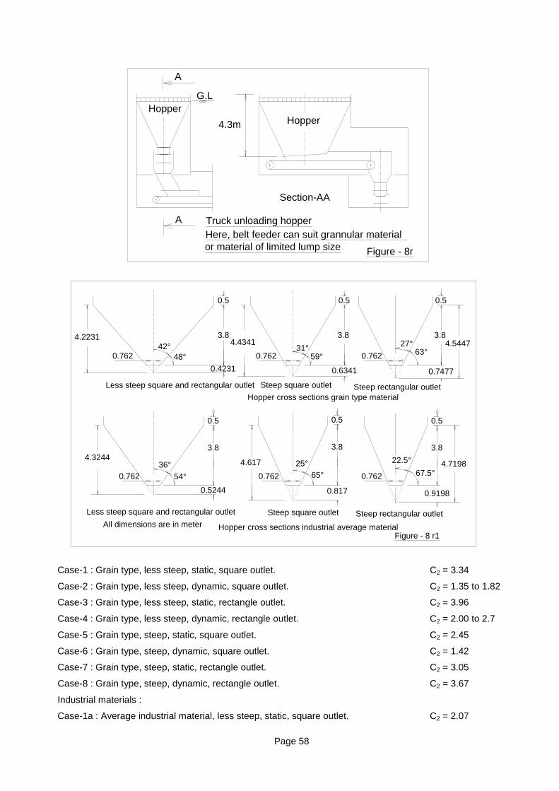
Page 58
Case-1 : Grain type, less steep, static, square outlet. C2 = 3.34
Case-2 : Grain type, less steep, dynamic, square outlet. C2 = 1.35 to 1.82
Case-3 : Grain type, less steep, static, rectangle outlet. C2 = 3.96
Case-4 : Grain type, less steep, dynamic, rectangle outlet. C2 = 2.00 to 2.7
Case-5 : Grain type, steep, static, square outlet. C2 = 2.45
Case-6 : Grain type, steep, dynamic, square outlet. C2 = 1.42
Case-7 : Grain type, steep, static, rectangle outlet. C2 = 3.05
Case-8 : Grain type, steep, dynamic, rectangle outlet. C2 = 3.67
Industrial materials :
Case-1a : Average industrial material, less steep, static, square outlet. C2 = 2.07
or material of limited lump size
A
Section-AA
A
Here, belt feeder can suit grannular material
4.3m Hopper
Figure - 8r
G.L
Hopper
Truck unloading hopper
67.5°65°54°
63°59°48°
Less steep square and rectangular outlet
Steep rectangular outlet
22.5°
27°
0.5
0.7477
0.9198
0.762
Steep rectangular outletSteep square outlet
Steep square outlet
25°
0.817
31°
All dimensions are in meter Hopper cross sections industrial average material
0.6341
0.5
3.8
0.5
0.5
Figure - 8 r1
0.5244
36°
42°
0.4231
3.8
Less steep square and rectangular outlet
Hopper cross sections grain type material
3.8 3.8
0.5
3.8
0.5
3.8
0.7620.762
0.762 0.762 0.762
4.22314.4341 4.5447
4.32444.617 4.7198
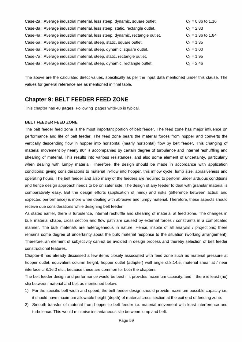
Page 59
Case-2a : Average industrial material, less steep, dynamic, square outlet. C2 = 0.86 to 1.16
Case-3a : Average industrial material, less steep, static, rectangle outlet. C2 = 2.83
Case-4a : Average industrial material, less steep, dynamic, rectangle outlet. C2 = 1.36 to 1.84
Case-5a : Average industrial material, steep, static, square outlet. C2 = 1.35
Case-6a : Average industrial material, steep, dynamic, square outlet. C2 = 1.00
Case-7a : Average industrial material, steep, static, rectangle outlet. C2 = 1.95
Case-8a : Average industrial material, steep, dynamic, rectangle outlet. C2 = 2.46
The above are the calculated direct values, specifically as per the input data mentioned under this clause. The
values for general reference are as mentioned in final table.
Chapter 9: BELT FEEDER FEED ZONE
This chapter has 48 pages. Following pages write-up is typical.
BELT FEEDER FEED ZONE
The belt feeder feed zone is the most important portion of belt feeder. The feed zone has major influence on
performance and life of belt feeder. The feed zone bears the material forces from hopper and converts the
vertically descending flow in hopper into horizontal (nearly horizontal) flow by belt feeder. This changing of
material movement by nearly 90° is accompanied by certain degree of turbulence and internal reshuffling and
shearing of material. This results into various resistances, and also some element of uncertainty, particularly
when dealing with lumpy material. Therefore, the design should be made in accordance with application
conditions; giving considerations to material in-flow into hopper, this inflow cycle, lump size, abrasiveness and
operating hours. The belt feeder and also many of the feeders are required to perform under arduous conditions
and hence design approach needs to be on safer side. The design of any feeder to deal with granular material is
comparatively easy. But the design efforts (application of mind) and risks (difference between actual and
expected performance) is more when dealing with abrasive and lumpy material. Therefore, these aspects should
receive due considerations while designing belt feeder.
As stated earlier, there is turbulence, internal reshuffle and shearing of material at feed zone. The changes in
bulk material shape, cross section and flow path are caused by external forces / constraints in a complicated
manner. The bulk materials are heterogeneous in nature. Hence, inspite of all analysis / projections; there
remains some degree of uncertainty about the bulk material response to the situation (working arrangement).
Therefore, an element of subjectivity cannot be avoided in design process and thereby selection of belt feeder
constructional features.
Chapter-8 has already discussed a few items closely associated with feed zone such as material pressure at
hopper outlet, equivalent column height, hopper outlet (adapter) wall angle cl.8.14.5, material shear at / near
interface cl.8.16.0 etc., because these are common for both the chapters.
The belt feeder design and performance would be best if it provides maximum capacity, and if there is least (no)
slip between material and belt as mentioned below.
1) For the specific belt width and speed, the belt feeder design should provide maximum possible capacity i.e.
it should have maximum allowable height (depth) of material cross section at the exit end of feeding zone.
2) Smooth transfer of material from hopper to belt feeder i.e. material movement with least interference and
turbulence. This would minimise instantaneous slip between lump and belt.

Page 60
3) Absence (or least) portion of feed zone subjected to „general‟ slip between material layer and belt. The slip
between material and belt is highly detrimental to belt life, particularly for lumpy and abrasive material. The
material layer is in dynamic (agitated) condition. The instantaneous slip between individual lump and belt
cannot be avoided altogether, due to mutual interference and intermeshing of lumps. The statement of sr.
no. 2 refers to instantaneous slip of localised nature. The statement of sr. no. 3 refers to „general‟ slip
between material layer portion as a whole, and belt.
4) Reasonably balanced flow across interface. Such flow balance is necessary for best performance of
combined system of hopper and belt feeder, particularly for large sized hopper. This has more reflection on
hopper performance and a system as a whole, and less as an individual item of belt feeder. This aspect has
been already discussed in chapter-7.
The material flow behaviour in feed zone, depends upon various forces action on bulk material in feed zone. If
the sum of propelling / pulling forces on specific body of bulk material, is sufficiently more than the sum of
resisting forces, then slip would be the least. The aim of this chapter is to calculate the various forces in feed
zone, and to know the effect of different parameters on these forces. Subsequently, this information can be
utilised to choose right parameters for belt feeder. The chapter progressively explains the feed zone issues, by
successive topics as below :
- Load equivalent model, cl.9.1.0 (for load from hopper).
- Bulk material block mass Me, cl. 9.2.0 (equivalent to load from hopper).
- Force transfer between two bodies in contact, cl. 9.3.0
- Pushing / ejecting force Fp1 at interface, cl.9.4.0
- Skirt board reaction force, Fp2, cl. 9.5.0
- Pulling / dragging force Fp3 on material due to belt (friction grip), cl. 9.6.0
- Material shear resistance, Fr1, cl. 9.7.1
- Frictional resistance Fr2 by skirt plates, cl. 9.7.2
- Material lift resistance Fr3 in feed zone, cl. 9.7.3
- Flow behaviour in feed zone, cl. 9.8.0
- Material general shear not at interface, cl.9.9.0
- Review general shear plane, cl. 9.9.3
BULK MATERIAL LOAD EQUIVALENT MODEL
As discussed in chapter-8 the material in hopper, exerts certain pressure at interface of hopper and belt feeder.
This pressure values multiplied by interface area, is the force exerted by material onto the belt feeder. The belt
feeders are mostly horizontal or will have shallow inclination (higher inclination is generally avoided, but is not
rule). So, the vertical pressure in bulk material has dominant effect, whereas the horizontal pressure effect is
insignificant. Therefore, the belt feeders are customarily designed considering that the material force (load) is
vertical, at interface.
The belt feeder design is concerned with magnitude of material force acting on belt feeder. It is convenient to
account for vertical force (load) on belt feeder, by considering bulk material block of equivalent height resting at
interface as shown in figure-9A, 9B, 9C and 9D. Thus in this equivalent model, although there is continuous
entity of bulk material of real height in hopper, but its actual effect on belt feeder is represented by material
region (block) freely standing on material layer on belt. There are no shear / frictional resistances on vertical

Page 61
sides of this block, and there is no downward pressure by material which is above this block. The four sides of
the block are vertical.
The block height is chosen such that its vertical force is equal to the actually occurring (expected) force in
particular application. This material block height in a specific application is proportionate to skirt board width, by
certain factor as discussed in chapter-8. This factor is named as C2, wherein :
Block height = C2 x (skirt board inside net width), at each point on feed zone length.
Now, belt feeder, can have skirt board of constant width, and it can also have expanding width of skirt board
(taper on width). For the skirt board of constant width, the block will also be of uniform height. In case of
expanding skirt board, the block height will also increase gradually (linearly).
Following figures show belt feeder along with feed zone and block of equivalent model, for various arrangements
of belt feeder.
Figure-9A : Horizontal belt feeder which has skirt board of constant width and constant height.
Figure-9B : Incline belt feeder which has skirt board of constant width and constant height.
Figure-9C : Horizontal belt feeder which has expanding width and expanding height of skirt board.
Figure-9D : Incline belt feeder which has expanding width and expanding height of skirt board.
Figure - 9A
Hopper
HeHi
Horizontal belt feeder,skirt board of constant width and height
A
A Section- AA
Equivaent
He
Elevation
block
Hopper
Equivalent
Section - BBB
B
Inclined belt feeder, skirt board of constant width and height
Hi
He
Hopper
Figure - 9B
He
Elevation
block
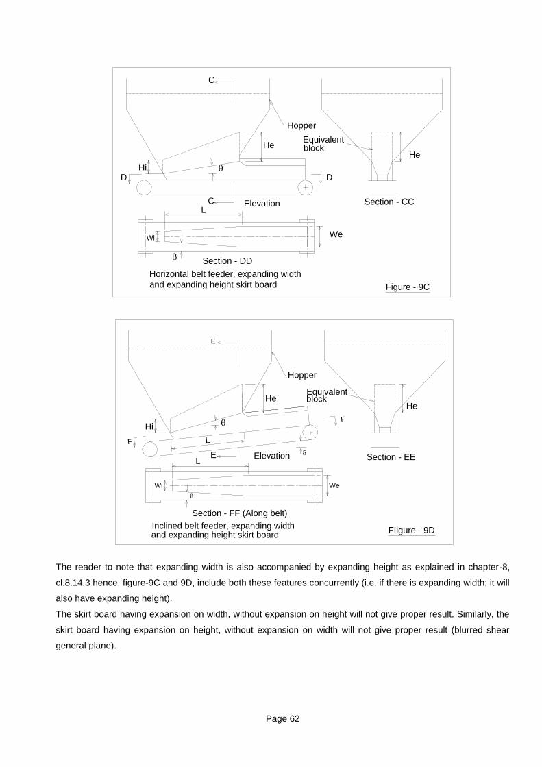
Page 62
The reader to note that expanding width is also accompanied by expanding height as explained in chapter-8,
cl.8.14.3 hence, figure-9C and 9D, include both these features concurrently (i.e. if there is expanding width; it will
also have expanding height).
The skirt board having expansion on width, without expansion on height will not give proper result. Similarly, the
skirt board having expansion on height, without expansion on width will not give proper result (blurred shear
general plane).
He
Equivalent
Section - CC
Hi
He
Hopper
Wi We
DD
Section - DD
C
C Elevation
Figure - 9C
L
block
and expanding height skirt board
Horizontal belt feeder, expanding width
FIigure - 9DInclined belt feeder, expanding width
ElevationE
E
Section - FF (Along belt)
F
F
WeWi
Hopper
He
Hi
Section - EE
blockHe
L
L
Equivalent
and expanding height skirt board

Page 63
SKIRT BOARD REACTION FORCE Fp2
The bulk material in skirt board and bulk material in
hopper has continuous entity. The effect of bulk
material in hopper is accounted by equivalent model as
per cl.-8.14.0 and cl.-9.1.0. Thus bulk material in skirt
board and bulk material of equivalent block are resting
on belt. The gravity force acting on this bulk material
creates presence of vertical pressure within
constrained body of bulk material. This vertical
pressure also creates the presence of horizontal
pressure within the body of bulk material as per
Rankine factor or horizontal pressure factor. The
Rankine factor has lower value and is considered here
to compensate for constrained space within which
material may not be able to spread effectively to
generate force. Thus bulk material resting on belt is in
pressurised state, vertically as well as horizontally.
The bulk material on belt is prevented from spreading by skirt plates. Therefore, material is continuously
applying thrust on skirt plates. The skirt plates are continuously applying reaction force on material. As would be
seen the reaction force from skirt plates creates pushing force on material and thereby belt, as shown
schematically in figure-9V. The situation is similar to a person standing on a roller surface and pushing wall. The
person would move away from the wall by equal force. If the skirt board is of constant width, then the reaction
force will be acting only from back plate, but the reaction force from side plates would cancel each other. In case
of expanding skirt board the reaction force will be exerted on material from back plate and also from side plates.
This topic decides the reaction force in following sequence :
- Reaction pushing force from back plate
- Reaction pushing force from side skirt plates
Pushing force Fp2a from back plate
This analysis considers belt being horizontal
and back plate perpendicular to belt i.e. back
plate in vertical plane. If the back plate is
inclined to vertical, it does not change situation
as its thrust direction remains horizontal.
However, material entering at rear end is
immediately tending to move forward. So, there
may not be enough pressure and reaction force
from back plate. This is subjective and is
accounted by multiplier factor 0.5 to calculated
value, for design safety.
Figure - 9V
Force acting
V
Belt
Force acting on wall
Force acting on belt
(At hands)
on wallForce acting
on material
Figure-9W
L
WeWi
Plan along belt
Reaction force on material
Material inskirt board
hopperMaterial in
he
He
Hi
hi
Elevation
Belt

Page 64
Referring to figure-9W, generally We, he, , and C2 are primary original dimension. The dimension hi, Wi, Hi
and He are secondary in nature (i.e. derived from primary dimension). So, result is derived with reference to exit
end dimension We and he.
We : Skirt board exit end, m
he : Skirt board material height at exit end, m
: Skirt board top face inclination to belt line
Ge : Vertical gradient interface appearing in elevation, Ge = tan
: Skirt plate side inclination to belt feeder centre line
Gp : Skirt plate width gradient per side, appearing in plan, Gp = tan
He : Material equivalent block height at exit end, m
C2 : Ratio of H W, which is constant. H = C2 . W, where W is skirt board width and H is block height at that
location.
: Material repose angle, degrees
Wi = We - 2 . Gp . L
hi = he - Ge . L
Hi = C2 . Wi = C2 . (We - 2 . Gp . L)
Rankine factor K = (1 - sin) (1 + sin)
Horizontal pressure at rear end, interface level = K . . g . Hi = K . . g . C2 . (We - 2 . Gp . L)
Horizontal pressure at rear end, belt level = K . . g . (hi + Hi)
= K . . g [ he - Ge . L + C2 . (We - 2 . Gp . L)]
Average horizontal pressure = 0.5 . K . . g . [he - Ge . L + C2 . (We - 2 . Gp . L) + C2 . (We - 2 . Gp . L)]
= K . . g . [0.5 . (he - Ge . L) + C2 . (We - 2 . Gp . L) ]
Area of back plate = hi . Wi = (he - Ge . L ) . (We - 2 . Gp . L)
Pushing force Fp2a = (Pressure) x (Area) x (Multiplier 0.5 for reduced pressure effect)
= 0.5 K . . g . [0.5 (he - Ge . L) + C2 . (We - 2 . Gp . L)] . (he - Ge . L) . (We - 2 . Gp . L) N
Alternatively,
If values of Wi, hi and C2 are known, then one can use following formula : Hi = C2. Wi
Horizontal pressure at rear end, interface level = K . . g . Hi = K . . g . C2 . Wi
Horizontal pressure at rear end, belt level = K . . g . (hi + Hi) = K . . g . (hi + C2 . Wi)
= K . . g . C2 . Wi + K . . g . hi
Average horizontal pressure = 0.5 [K . . g . C2 . Wi + K . . g . C2 . Wi + K . . g . hi]
= 0.5 . K . . g . (hi + 2 . C2 . Wi)
Area = hi . Wi
Pushing force Fp2a = hi . Wi x 0.5 . K . . g . (hi + 2 . C2 . Wi) x (multiplier 0.5)
= 0.25 . K . . g . hi . Wi . (hi + 2 . C2 . Wi)
The above multiplier 0.5 is for possibility of inadequate pressure between material and back plate.

Page 65
Pushing force Fp2b from skirt board sides
Figure-9X middle portion and top portion
schematically shows the material in skirt board and
material equivalent in hopper. Belt line AA‟ is inclined
at angle to horizontal. Line AB and A‟B‟ are inclined
at angle to vertical. Lines BC and B‟C‟ are vertical.
So line ABC and A‟B‟C‟ are not straight but are
deviating by angle . Normally value being small
these lines have been considered as vertical. So,
material pressure at point A‟ will be corresponding to
height A‟B‟ + B‟C‟. The inaccuracy in result could be
up to 3% or accuracy of calculation would be around
97%, which is adequate for engineering need. The
derivation is based on figure-9X bottom portion.
The calculation can be made by integration and
elaborate method, but the same would result into
lengthy formula and inconvenient to use. It is
sufficient to consider material side pressure as an
average of side pressure at points A, B, B‟ and A‟,
and then multiply it by skirt plate area to know
pressing / reaction force. Hence, this method has
been used.
Nomenclature :
We : Skirt board width at exit end, m
he : Skirt board height exit end, m
: Skirt board top face inclination to belt,
degree; Ge = tan
: Skirt plate inclination to belt feeder centre line, degree; Gp = tan
C2 : Material column factor, (constant along feed length)
L : Feed zone length along belt, m
Fn : Force perpendicular to skirt plates, N
: Material repose angle, degree
Based on above :
Wi = We - 2 . Gp . L
hi = he - Ge . L
He = C2 . We
Hi = C2 . Wi = C2 . (We - 2 . Gp . L)
Rankine factor K = (1 - sin) (1 + sin)
Side pressure at A = K . . g . (hi + Hi) = K . . g . [he - Ge . L + C2 . (We - 2 . Gp . L)]
Side pressure at B = K . . g . Hi = K . . g . C2 . (We - 2 . Gp . L)
Side pressure at B‟ = K . . g . He = K . . g . C2 . We
L
x
hx
Hx
D
dx
V
he
Belt
Elevation
Hi
He
he
hi E
L
C'
B'
A'
C
B
A
Fn
Wi
hi
Figure-9X
We
Plan along belt
Material inskirt board
hopperMaterial in
He
Hi
Elevation
Belt
V
Fn
Page 66
Side pressure at A‟ = K . . g . (He + he) = K . . g . (C2 . We + he)
Average side pressure perpendicular to skirt plates :
= 0.25 K . . g . [he - Ge . L + C2 . We - 2 . C2 . Gp . L + C2. We - 2 . C2 . Gp . L + C2 . We + C2 . We + he]
= 0.25 . K . . g . (2 . he + 4 C2 . We - Ge . L - 4 . C2 . Gp . L) N/m2
Each skirt plate area = 0.5 (he + hi) . L
(he and hi are actually perpendicular to L, although not in figure portion referred for derivation. The issue is
insignificant for engineering calculations).
Each skirt plate area = 0.5 . (he + he - Ge . L) . L = 0.5 . (2 . he - Ge . L) . L
The force on each skirt plate is the average pressure multiplied by area. This fore is perpendicular to skirt plates
as per Rankine factor. The force perpendicular to each skirt plate is Fn.
Fn = 0.125 K . . g . L . (2 he - Ge . L) . (2 . he + 4 C2 . We - Ge . L - 4 . C2 . Gp . L) N
Pushing force, Fp2b = 2 . Fn . sin
Fp2b = 0.25 K . . g . L . (2 he - Ge . L) . (2 . he + 4 C2 . We - Ge . L - 4 . C2 . Gp . L) . sin N
FLOW BEHAVIOUR IN FEED ZONE
The purpose of this chapter is to look into the qualitative aspects of material flow in feed zone. In this context,
foregoing topics cl.9.4.0, 9.5.0 and 9.6.0 enable to calculate following forward forces which are trying to move
the entire material in feed zone, in direction of belt travel (the entire body implies as if shear is taking place at
interface).
- Ejecting / pushing force Fp1 at interface
- Skirt-board reaction force Fp2
- Pulling / dragging force Fp3 by belt
The sum of these forward forces is Fp = Fp1 + Fp2 + Fp3
The foregoing topics cl.9.7.1, 9.7.2 and 9.7.3 enable to calculate following resistances which are opposing the
motion of entire body of material, along belt, in feed zone (the entire body implies as if shear is taking place at
interface).
- Material shear resistance Fr1 from interface
- Skirt board frictional resistance Fr2
- Material lift resistance Fr3
The sum of resistances (backward forces), Fr = Fr1 + Fr2 + Fr3
It is obvious that if Fp > Fr; then the entire body of material in skirt board will move forward (as applicable to belt
feeder), as general shear along interface.
However, if Fp < Fr; then entire body of material will not move forward, in singular mode. The shear will be
occurring at plane which is more sloping, compared to interface i.e. shear plane angle ‟ is greater than interface
angle . The magnitude of ‟ is such that its Fp‟ > Fr‟. The material ahead of such shear plane will move forward
at regular pace, but material behind this shear plane will have sluggish forward motion, with more rubbing and
abrasion on belt. Thus, this analysis provides the projected (likely) flow behaviour in feed zone. This analysis is
to be utilised to determine / revise / refine the important parameters during design stage, as per following hints.
1) If the material is very abrasive or damaging in nature, then it is preferred that Fp > Fr, with respect to entire
feed zone. Thus, designer should try to select feeder parameters in such application so as to have Fp > Fr

Page 67
or shear plane at least touching the junction of belt and back plate of skirt board. In the event if this is not
feasible, then expect more wear of belt.
2) In case of non abrasive material, the shear plane termination before back plate can be tolerated, but still one
can take some remedial measures such as comparatively less speed etc.
3) It would be observed that when material is under high pressure accompanied by tall skirt board, the same
demands higher value of and for shear at interface, for proper position of shear plane. This would result
into comparatively lesser length of feed zone, to have optimum belt life.
4) When the material is under high pressure and material is very damaging to belt (very abrasive, large lumps,
sharp edges, etc) it is desirable that feed zone is restricted such that shear plane extends to and above the
mid height of back plate, for proper life of belt. Such application can be tackled by feed zone of lesser length.
5) The shallow hopper can have shear at interface or close to interface, making it possible to have long feed
zone length.
6) Thus this chapter analysis provides important hint / suggestions to review feed zone length, layout, belt
speed etc. on case to case basis. The analysis also enables to recalculate flow balance condition in feed
zone.
7) Flow balance review can be made by using the flow balance tables as below :
For shear at interface, use value of ZT% from table.
For shear plane intersecting back plate, read value of ZT% from table, for and ‟. The ZT% can be
considered 1.05 ZT% of table.
For shear plane intersecting belt, see value of ZT% from table, for and ‟. The ZT% can be considered
1.1 ZT% of table, corresponding to applicable active length of feed zone.
The aforesaid additional factors are for opportunistic additional inflow in rear sluggish portion, which would
be particularly a case when shear plane is directly intersecting the belt, and material behind this plane is
trying to enter in to the active zone.
For the application which is very sensitive to flow balance, one has to calculate the flow distribution for the
applicable shear plane (whether at interface or at other plane) when tabulated values are not matching with
the applicable values. The designer is to refer the earlier chapter-7, which describes the calculation
procedure.
8) It is clarified that flow balance at interface is of secondary importance, for transitional hoppers (such as for
pay loader, reclaim hopper, truck unloading, wagon unloading etc.), because the flow from such hoppers is
of cyclic nature. In case of unbalanced flow distribution at interface the belt feeder will tend to take more
material from particular zone where level is high, however, as this level drops in each cycle, it will draw the
material automatically from other zone (where material is present). Thus cyclic inflow in hopper will ensue
its reasonable emptying from every side, in each cycle of few minutes (or 10 / 15 minutes). Thus making the
flow balance issue of secondary nature. In such hoppers, the primary consideration should be to use and
such that same result into least rubbing between material and belt i.e. shear at interface or shear plane
intersecting back plate or minimum space between back plate and shear plane, when dealing with difficult
materials.
9) Shear plane angle ‟ (which happens to be greater than ) results in to functionally deep type adapter
(extending its function into skirt board). The deep type adapter does not alter pressure pattern and C2 at
interface.

Page 68
Example-6
Calculate value of Fp and Fr in feed zone, assuming shear at interface, for following application :
he = 0.82 m, hi = 0.27 m, He = 0.938 x 3 = 2.81m, Hi = 0.4 x 3 = 1.2 m, We = 0.938 m
Wi = 0.4m, = 5.710593°, Ge = 0.1, = 2.8°, Gp = 0.0489, L = 5.5 m,
= 2°, C2 = 3, = 36°, s = 0.423, Qd = 480 mtph, b = m = 0.6346, = 1000 kg/m3
Belt velocity V = 0.23 mps.
Then also check whether assumption is correct.
Solution
Firstly, this requires calculation of material block mass above interface
= 16432.36 x 0.471739 = 7751.789 kg
F = 7751.789 x 9.81 = 76045 N
Fp1= F. [cos ( + )]. sin = 76045 x cos 7.710593 x sin 5.710593 = 7498.3 N
K = (1 - sin) (1 + sin) = (1 - sin 36) (1 + sin36) = 0.2596
Fp2 = 0.25 . K . . g . hi . Wi . (hi + 2 . C2 . Wi) + 0.25 K . . g . L . (2 he - Ge . L) . (2 . he + 4 C2 . We - Ge . L - 4
. C2 . Gp . L) . sin
Fp2 = 0.25 x 0.2596 x 1000 x 9.81 x 0.27 x 0.4 x (0.27 + 2 x 3 x 0.4) + 0.25 x 0.2596 x 1000 x 9.81 x 5.5 x (2
x 0.82 - 0.1 x 5.5) x (2 x 0.82 + 4 x 3 x 0.938 - 0.1 x 5.5 - 4 x 3 x 0.0489 x 5.5) x sin2.8
Fp2 = 183.6 + 1700.1 = 1883.7 N
Material mass Ms in skirt board
Ms = . [6 he . We . L - 3 (Ge . We + 2 Gp . he) . L2 + 4 Ge . Gp . L
3] 6
= 1000 x [6 x 0.82 x 0.938 x 5.5 - 3 x (0.1 x 0.938 + 2 x 0.0489 x 0.82) x 5.52 + 4 x 0.1 x 0.0489 x 5.5
3] 6
= 1000 x [25.3822 - 15.7901 + 3.2542] 6 = 2141.05 kg
Fp3 = b . F . [cos( + )] . [cos + m . sin] + b . Ms . g . cos
Fp3 = 0.6346 x 76045 x [cos7.710593] x [cos5.710593 + 0.6346 x sin 5.710593] + 0.6346 x 2141.05 x 9.81 x
cos2
= 47822.4 x 1.058182 + 13320.8
Fp3 = 63925.6 N
Total propelling force Fp = Fp1 + Fp2 + Fp3 = 7498.3 + 1883.7 + 63925.6 = 73307.6 N
Fr1 = m . F . [cos( + )] . cos
= 0.6346 x 76045 x cos7.7105983 x cos 5.710593
Fr1 = 47584.5 N
Fr2 = 0.25 s . K . . g . L . (2 he - Ge . L) . (2 . he + 4 C2 . We - Ge . L - 4 . C2 . Gp . L) N
= 0.25 x 0.423 x 0.2596 x 1000 x 9.81 x 5.5 x (2 x 0.82 - 0.1 x 5.5) x (2 x 0.82 + 4 x 3 x 0.938 - 0.1 x 5.5 - 4 x 3 x
0.0489 x 5.5) N
= 1481.21 x 1.09 x 9.1186 = 14722.1 N
Fr3 = Qd . g. hf (3.6 V)
hf = (0.5 x 5.5) sin2 = 0.095974 m
222
2222
5.5x1.0x3
45.5x938.0x0489.0x2938.0.
710593.5cos
5.5x7105.7cos3x1000MeMass
L.Gp3
4L.We.Gp2We.
cos
L.cosC.MeMass

Page 69
Fr3 = 480 x 9.81 x 0.095974 (3.6 x 0.23) = 546 N
Total resistance Fr = Fr1 + Fr2 +Fr3 = 47584.5 + 14722.1 + 546 = 62852.6 N
Thus Fp > Fr by sufficient margin (at least 1.07 times) and material general shear can be said as occurring at
interface. It would be observed that in well-designed belt feeder of expanding cross section type, it is often
possible to have general shear at interface. Thus assumption is correct and material shear is at interface.
MATERIAL GENERAL SHEAR NOT AT INTERFACE
The formulae in foregoing cl. 9.4.0, 9.5.0, 9.6.0
and 9.7.0 are for calculating propelling force
and resistance when material shear is at
interface. Now on calculating Fp and Fr on the
basis of shear at interface, it might happen that
Fp as above is not larger than 1.07Fr as above.
This means material general shear will not
occur at interface, but will be occurring at a
plane more inclined than interface. The
designer would like to know the probable
position of this shear plane. This topic
discusses and derives the likely position of such
plane for general shear.
There are two possibilities viz. case-1 and case-
2 as below :
Case-1 : Referring to figure-9c, the shear plane
is intersecting back plate.
Case-2 : Referring to figure-9d, the shear plane
is lower than back plate and is directly
intersecting the belt within feed zone.
There are two distinct formulae for case-1 and
case-2; to decide value of ‟(i.e. angle of shear plane to belt).
The designer to proceed in following sequence to decide location of general shear plane:
1) First check whether shear is occurring at interface, as per foregoing clauses and examples-6 & 7 on the
basis of values of Fp and Fr.
2) If Fp is not larger than 1.07Fr as per serial no.1; then use formula of case-1. The cas-1 formula can be used
for ‟ value maximum, till it touches point A of figure-9c.
‟ maximum value = tan-1
(he L)
< ‟ < tan-1
(he L)
3) If Fp is still not larger than 1.07Fr as per serial no. 2 above; then use formula of case-2. In this case ‟ has
limitation as below :
tan-1
(he L) < ‟ < 90°
One will rarely cross 10 to 15 degree. However, this formula can enable to see the flow pattern at unlimited
points within feed zone by choosing different values of ‟.
Fn
Belt
Elevation
Hi
HeMaterial inhopper
skirt boardMaterial in
Plan along belt
We
Figure-9c
hi
Wi
Fn
A
B
C
A'
B'
C'
L
he
V
'D
Case-1
Page 70
Case-1 : Shear plane intersecting back plate
Suppose shear plane is inclined at ‟ such that it is intersecting back plate as shown in figure-9c. The suffix ( „ )
relates to values corresponding to ‟, such as Ge‟ = tan‟ etc. Firstly, the calculation requires the value of mass
M1 of block DBB‟. This block is in the form of wedge. Its mass is given by following formula :
BD = BA - AD = (he - L . tan) - (he - L . tan‟) = L . (tan‟ - tan) = L . (Ge‟ - Ge)
M1 = . (BD) . L . (Wi + Wi + We) 6
= . L . (Ge‟ - Ge) . L . (We - 2 . Gp . L + We - 2 . Gp . L + We) 6
= . L2 . (Ge‟ - Ge) . (3 . We - 4 . Gp . L) 6
Now, to decide shear plane, one has to choose value of ‟ such that it satisfies following equation, by sufficient
margin (i.e. factor 1.07 based on engineering judgement).
Fp1 + Fp2a + Fp2b + Fp3 Fr1 + Fr2 + Fr3
The end result cannot be converted into simple short formula. Each of propelling force and resistance to be
calculated as below and see that which value of ‟ makes them nearly equal. This exercise is very quick and
simple by use of computer.
Fp1 : This is pushing force on incline shear plane
Fp1 = F‟ . [cos( + ‟)] . sin‟ N (similar to cl. 9.4.2)
Here, F‟ = (Block mass BB‟C‟C + block mass DBB‟) . g = (Me + M1) . g
Me value as per cl. 9.2.0 and M1 value as mentioned in this topic.
Fp2a : This is reaction force from skirt board back side, directly acting on material in motion.
hi‟ = he - L . tan‟ = he - Ge‟ . L
Wi‟ = Wi = We - 2 . Gp . L
Vertical pressure at A = . g . (Hi + hi) = . g . (C2 . Wi + he - Ge . L)
= . g . [C2(We - 2 . Gp . L) + he - Ge . L]
Vertical pressure D = . g . (Hi + BD) = . g . [C2 . (We - 2 . Gp . L) + L . (Ge‟ - Ge)]
Average vertical pressure = 0.5 . . g . [2 . C2 . (We - 2 . Gp . L) + he - Ge . L + L . (Ge‟ - Ge)]
The belt is tending to carry forward material near back plate. So, there may not be enough pressure. This is
accounted by multiplying by 0.5 in the formula as below :
Fp2a = K . (hi‟. Wi) . 0.5 . . g . [2 . C2 . (We - 2 . Gp . L) + he - Ge . L + L . (Ge‟ - Ge)] x 0.5
= 0.25 . K . . g . (hi‟. Wi) . [2 . C2 . (We - 2 . Gp . L) + he - Ge . L + L . (Ge‟ - Ge)] N
Fp2b : This is reaction force from skirt board sides, directly acting on material in motion. The vertical pressure
on skirt board can be considered as an average of vertical pressure at points A, D, B‟ and A‟.
Vertical pressure at A = . g . [C2(We - 2 . Gp . L) + he - Ge . L]
Vertical pressure at D = . g . [C2 . (We - 2 . Gp . L) + L . (Ge‟ - Ge)]
Vertical pressure at B‟ = . g . He = . g . C2 . We
Vertical pressure at A‟ = . g . (He + he) = . g . [C2 . We + he]
Avg. vertical pressure = 0.25 . g . [2 C2 (We - 2 . Gp . L) + he - Ge . L + L . (Ge‟ - Ge) + 2 C2 . We + he]
Area of each skirt plate for pressure = 0.5 (AD + he) . L = 0.5 (he - Ge‟ . L + he) . L
= 0.5 (2 he - Ge‟ . L) . L
The area of two skirt plates = (2 he - Ge‟ . L) . L
Fp2b = 0.25 K. . g . L [(2 he - Ge‟ . L)] . [2 C2 (We - 2 . Gp . L) + he - Ge . L + L . (Ge‟ - Ge) + 2 C2 . We + he] .
sin
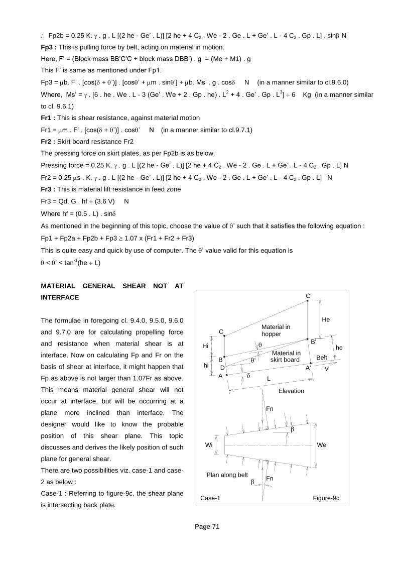
Page 71
Fp2b = 0.25 K. . g . L [(2 he - Ge‟ . L)] [2 he + 4 C2 . We - 2 . Ge . L + Ge‟ . L - 4 C2 . Gp . L] . sin N
Fp3 : This is pulling force by belt, acting on material in motion.
Here, F‟ = (Block mass BB‟C‟C + block mass DBB‟) . g = (Me + M1) . g
This F‟ is same as mentioned under Fp1.
Fp3 = b. F‟ . [cos( + ‟)] . [cos‟ + m . sin‟] + b. Ms‟ . g . cos N (in a manner similar to cl.9.6.0)
Where, Ms‟ = . [6 . he . We . L - 3 (Ge‟ . We + 2 . Gp . he) . L2 + 4 . Ge‟ . Gp . L
3] 6 Kg (in a manner similar
to cl. 9.6.1)
Fr1 : This is shear resistance, against material motion
Fr1 = m . F‟ . [cos( + ‟)] . cos‟ N (in a manner similar to cl.9.7.1)
Fr2 : Skirt board resistance Fr2
The pressing force on skirt plates, as per Fp2b is as below.
Pressing force = 0.25 K. . g . L [(2 he - Ge‟ . L)] [2 he + 4 C2 . We - 2 . Ge . L + Ge‟ . L - 4 C2 . Gp . L] N
Fr2 = 0.25 s . K. . g . L [(2 he - Ge‟ . L)] [2 he + 4 C2 . We - 2 . Ge . L + Ge‟ . L - 4 C2 . Gp . L] N
Fr3 : This is material lift resistance in feed zone
Fr3 = Qd. G . hf (3.6 V) N
Where hf = (0.5 . L) . sin
As mentioned in the beginning of this topic, choose the value of ‟ such that it satisfies the following equation :
Fp1 + Fp2a + Fp2b + Fp3 1.07 x (Fr1 + Fr2 + Fr3)
This is quite easy and quick by use of computer. The ‟ value valid for this equation is
< ‟ < tan-1
(he L)
MATERIAL GENERAL SHEAR NOT AT
INTERFACE
The formulae in foregoing cl. 9.4.0, 9.5.0, 9.6.0
and 9.7.0 are for calculating propelling force
and resistance when material shear is at
interface. Now on calculating Fp and Fr on the
basis of shear at interface, it might happen that
Fp as above is not larger than 1.07Fr as above.
This means material general shear will not
occur at interface, but will be occurring at a
plane more inclined than interface. The
designer would like to know the probable
position of this shear plane. This topic
discusses and derives the likely position of such
plane for general shear.
There are two possibilities viz. case-1 and case-
2 as below :
Case-1 : Referring to figure-9c, the shear plane
is intersecting back plate.
Fn
Belt
Elevation
Hi
HeMaterial inhopper
skirt boardMaterial in
Plan along belt
We
Figure-9c
hi
Wi
Fn
A
B
C
A'
B'
C'
L
he
V
'D
Case-1

Page 72
Case-2 : Referring to figure-9d, the shear plane is lower than back plate and is directly intersecting the belt
within feed zone.
There are two distinct formulae for case-1 and case-2; to decide value of ‟(i.e. angle of shear plane to belt).
The designer to proceed in following sequence to decide location of general shear plane:
4) First check whether shear is occurring at interface, as per foregoing clauses and examples-6 & 7 on the
basis of values of Fp and Fr.
5) If Fp is not larger than 1.07Fr as per serial no.1; then use formula of case-1. The cas-1 formula can be used
for ‟ value maximum, till it touches point A of figure-9c.
‟ maximum value = tan-1
(he L)
< ‟ < tan-1
(he L)
6) If Fp is still not larger than 1.07Fr as per serial no. 2 above; then use formula of case-2. In this case ‟ has
limitation as below :
tan-1
(he L) < ‟ < 90°
One will rarely cross 10 to 15 degree. However, this formula can enable to see the flow pattern at unlimited
points within feed zone by choosing different values of ‟.
Case-1 : Shear plane intersecting back plate
Suppose shear plane is inclined at ‟ such that it is intersecting back plate as shown in figure-9c. The suffix ( „ )
relates to values corresponding to ‟, such as Ge‟ = tan‟ etc. Firstly, the calculation requires the value of mass
M1 of block DBB‟. This block is in the form of wedge. Its mass is given by following formula :
BD = BA - AD = (he - L . tan) - (he - L . tan‟) = L . (tan‟ - tan) = L . (Ge‟ - Ge)
M1 = . (BD) . L . (Wi + Wi + We) 6
= . L . (Ge‟ - Ge) . L . (We - 2 . Gp . L + We - 2 . Gp . L + We) 6
= . L2 . (Ge‟ - Ge) . (3 . We - 4 . Gp . L) 6
Now, to decide shear plane, one has to choose value of ‟ such that it satisfies following equation, by sufficient
margin (i.e. factor 1.07 based on engineering judgement).
Fp1 + Fp2a + Fp2b + Fp3 Fr1 + Fr2 + Fr3
The end result cannot be converted into simple short formula. Each of propelling force and resistance to be
calculated as below and see that which value of ‟ makes them nearly equal. This exercise is very quick and
simple by use of computer.
Fp1 : This is pushing force on incline shear plane
Fp1 = F‟ . [cos( + ‟)] . sin‟ N (similar to cl. 9.4.2)
Here, F‟ = (Block mass BB‟C‟C + block mass DBB‟) . g = (Me + M1) . g
Me value as per cl. 9.2.0 and M1 value as mentioned in this topic.
Fp2a : This is reaction force from skirt board back side, directly acting on material in motion.
hi‟ = he - L . tan‟ = he - Ge‟ . L
Wi‟ = Wi = We - 2 . Gp . L
Vertical pressure at A = . g . (Hi + hi) = . g . (C2 . Wi + he - Ge . L)
= . g . [C2(We - 2 . Gp . L) + he - Ge . L]
Vertical pressure D = . g . (Hi + BD) = . g . [C2 . (We - 2 . Gp . L) + L . (Ge‟ - Ge)]
Average vertical pressure = 0.5 . . g . [2 . C2 . (We - 2 . Gp . L) + he - Ge . L + L . (Ge‟ - Ge)]

Page 73
The belt is tending to carry forward material near back plate. So, there may not be enough pressure. This is
accounted by multiplying by 0.5 in the formula as below :
Fp2a = K . (hi‟. Wi) . 0.5 . . g . [2 . C2 . (We - 2 . Gp . L) + he - Ge . L + L . (Ge‟ - Ge)] x 0.5
= 0.25 . K . . g . (hi‟. Wi) . [2 . C2 . (We - 2 . Gp . L) + he - Ge . L + L . (Ge‟ - Ge)] N
Fp2b : This is reaction force from skirt board sides, directly acting on material in motion. The vertical pressure
on skirt board can be considered as an average of vertical pressure at points A, D, B‟ and A‟.
Vertical pressure at A = . g . [C2(We - 2 . Gp . L) + he - Ge . L]
Vertical pressure at D = . g . [C2 . (We - 2 . Gp . L) + L . (Ge‟ - Ge)]
Vertical pressure at B‟ = . g . He = . g . C2 . We
Vertical pressure at A‟ = . g . (He + he) = . g . [C2 . We + he]
Avg. vertical pressure = 0.25 . g . [2 C2 (We - 2 . Gp . L) + he - Ge . L + L . (Ge‟ - Ge) + 2 C2 . We + he]
Area of each skirt plate for pressure = 0.5 (AD + he) . L = 0.5 (he - Ge‟ . L + he) . L
= 0.5 (2 he - Ge‟ . L) . L
The area of two skirt plates = (2 he - Ge‟ . L) . L
Fp2b = 0.25 K. . g . L [(2 he - Ge‟ . L)] . [2 C2 (We - 2 . Gp . L) + he - Ge . L + L . (Ge‟ - Ge) + 2 C2 . We + he] .
sin
Fp2b = 0.25 K. . g . L [(2 he - Ge‟ . L)] [2 he + 4 C2 . We - 2 . Ge . L + Ge‟ . L - 4 C2 . Gp . L] . sin N
Fp3 : This is pulling force by belt, acting on material in motion.
Here, F‟ = (Block mass BB‟C‟C + block mass DBB‟) . g = (Me + M1) . g
This F‟ is same as mentioned under Fp1.
Fp3 = b. F‟ . [cos( + ‟)] . [cos‟ + m . sin‟] + b. Ms‟ . g . cos N (in a manner similar to cl.9.6.0)
Where, Ms‟ = . [6 . he . We . L - 3 (Ge‟ . We + 2 . Gp . he) . L2 + 4 . Ge‟ . Gp . L
3] 6 Kg (in a manner similar
to cl. 9.6.1)
Fr1 : This is shear resistance, against material motion
Fr1 = m . F‟ . [cos( + ‟)] . cos‟ N (in a manner similar to cl.9.7.1)
Fr2 : Skirt board resistance Fr2
The pressing force on skirt plates, as per Fp2b is as below.
Pressing force = 0.25 K. . g . L [(2 he - Ge‟ . L)] [2 he + 4 C2 . We - 2 . Ge . L + Ge‟ . L - 4 C2 . Gp . L] N
Fr2 = 0.25 s . K. . g . L [(2 he - Ge‟ . L)] [2 he + 4 C2 . We - 2 . Ge . L + Ge‟ . L - 4 C2 . Gp . L] N
Fr3 : This is material lift resistance in feed zone
Fr3 = Qd. G . hf (3.6 V) N
Where hf = (0.5 . L) . sin
As mentioned in the beginning of this topic, choose the value of ‟ such that it satisfies the following equation :
Fp1 + Fp2a + Fp2b + Fp3 1.07 x (Fr1 + Fr2 + Fr3)
This is quite easy and quick by use of computer. The ‟ value valid for this equation is
< ‟ < tan-1
(he L)
In the foregoing derivation, we have considered shear plane commencing exactly at exit point, to avoid
complexities in formula. Actually, it starts somewhat behind the exit point. Use the value of ‟ as per this
derivation and draw this shear plane at angle ‟ from its actual starting point and see how long is the „directly‟
active feed zone. This would provide engineering assessment of flow pattern in feed zone, which is the purpose
of knowing the shear plane position. Thereby, the engineering judgement for magnitude of abrasion, velocity

Page 74
gradient, average velocity etc. for comparative decision. The actual starting point of shear plane can be
considered as below.
Distance from exit point : 1.25 x (skirt board width), for grain type free flowing granular materials.
Distance from exit point : 0.75 x (skirt board width), for other materials.
Case-2 : Shear plane not reaching back plate
Assuming shear at interface and using their
applicable formula, if Fp < 1.07 Fr; then
assumption is not correct and designer has to
investigate as per case-1. If Fp is still less
than 1.07 Fr by using the formula as per case-
1; then designer has to try for the next stage
and use formulae as per this cl.9.9.2, to
decide the value of ‟ and thereby the position
of general shear plane.
This pattern of material shear in skirt board
can arise for deep material layer, high
pressure at interface, unfavorable value of
friction coefficients, very long feed zone,
inadequate gradients of skirt board expansion.
In this pattern; the shear plane is not reaching
the back plate. In actual examples, it would be
observed that this pattern of shear occurs less
frequently.
The hopper material pressure at interface
remains unchanged, and part of skirt board
functions as „deep type‟ adapter.
Figure-9d shows the skirt board elevation view. The belt feeder parameters are such that drag along bottom is
unable to move full mass in skirt board. In this situation, the dragging force at bottom will disintegrate material
body, creating its separation along line AB. The point-B will be located such that propelling forces sum is equal
(somewhat greater) than the resistance to motion of material body ABC. The material outside of ABC will
continuously add into active zone ABC. For the material body ABC; the dragging force in rear portion is
sufficiently more compared to its resistance at rear side. So this more pushing force from rear will tend to keep
the triangle intact for forward motion (i.e. it will avoid / reduce auxiliary shear lines within the said triangle). This
analysis derives the formula to decide the plane of general shear, in applicable cases.
Refer book for derivation of case-2.
Example-8
Calculate shear plane location in feed zone of 1400 mm belt feeder of following data :
We = 0.94 m, Wi = 0.687 m, he = 0.9 m, hi = 0.79 m, C2 = 4, He = 0.94 x 4 = 3.76 m,
Hi = 0.687 x 4 = 2.748 m, L = 5.5 m, = 1.145763°, Ge = 0.02, = 1.31757°,
Gp = 0.023, = 2°, = 34°, s = 0.45, b = m = 0.5914, = 1000 kg/m3,
Case-2
D
' V
he
L
F
A
C
BA
Fn
Wi
hi
Figure-9d
We
Plan along belt
Material inskirt board
hopperMaterial in
He
Hi
Elevation
Belt
Fn
E
Hx
hx
Wx

Page 75
Qd = 500 mtph, V = 0.22 mps
The data have been intentionally selected so that calculation passes through different stages. and
corresponds to adapter wall angle 1 22.5° (i.e. 67.5° from horizontal).
Solution
Checking whether general shear at interface.
= 14657 kg
Material mass Ms in skirt board
Ms = . [6 he . We . L - 3 (Ge . We + 2 Gp . he) . L2 + 4 Ge . Gp . L
3] 6
= 1000 x [6 x 0.9 x 0.94 x 5.5 - 3 x (0.02 x 0.94 + 2 x 0.023 x 0.9) x 5.52 + 4 x 0.02 x 0.023 x 5.5
3] 6
= 3793.5 kg
F = Me x 9.81 = 14657 x 9.81 = 143785 N
Fp1= F. [cos ( + )]. sin = 143785 x cos 3.145763 x sin 1.145763 = 2871 N
K = (1 - sin) (1 + sin) = (1 - sin34) (1 + sin34) = 0.2827
Fp2a = 0.25 . K . . g . hi . Wi . (hi + 2 . C2 . Wi)
= 0.25 x 0.2827 x 1000 x 9.81 x 0.79 x 0.687 x (0.79 + 2 x 4 x 0.687) = 2366 N
Fp2b = 0.25 K . . g . L . (2 he - Ge . L) . (2 . he + 4 C2 . We - Ge . L - 4 . C2 . Gp . L) . sin
= 0.25 x 0.2827 x 1000 x 9.81 x 5.5 x (2 x 0.9 - 0.02 x 5.5) x (2 x 0.9 + 4 x 4 x 0.94 - 0.02 x 5.5 - 4
x 4 x 0.023 x 5.5) x sin1.31757
= 6444.42 x 0.338148 = 2179 N
Fp2 = 2366 + 2179 = 4545 N
Fp3 = b . F . [cos( + )] . [cos + m . sin] + b . Ms . g . cos
Fp3 = 0.5914 x 143785 x [cos3.145763] x [cos1.145763 + 0.5914 x sin 1.145763] + 0.5914 x 3793.5 x
9.81 x cos 2
= 84906.41 x 1.011625697 + 21995.09 = 107888 N
Total propelling force Fp = Fp1 + Fp2 + Fp3 = 2871 + 4545 + 107888 = 115304 N
Fr1 = m . F . [cos( + )] . cos
= 0.5914 x 143785 x cos 3.145763 x cos 1.145763
= 84889 N
Fr2 = 0.25 s . K . . g . L . (2 he - Ge . L) . (2 . he + 4 C2 . We - Ge . L - 4 . C2 . Gp . L)
= 0.25 x 0.45 x 0.2827 x 1000 x 9.81 x 5.5 x (2 x 0.9 - 0.02 x 5.5) x (2 x 0.9 + 4 x 4 x 0.94 - 0.02 x 5.5 –
4 x 4 x 0.023 x 5.5) = 42647 N
Fr3 = Qd . g. hf (3.6 V)
hf = (0.5 x 5.5) sin 2 = 0.09597 m
Fr3 = 500 x 9.81 x 0.09597 (3.6 x 0.22) = 594 N
Total resistance Fr = Fr1 + Fr2 +Fr3 = 84889 + 42647 + 594 = 128130 N
Thus Fp < 1.07 Fr, and therefore shear plane is not at interface. Hence we have to try for shear plane by next
stage calculation (i.e. Case-1).
222
2222
5.5x023.0x3
45.5x94.0x023.0x294.0x
145763.1cos
5.5x145763.3cos4x1000Me
L.Gp3
4L.We.Gp2We.
cos
L.cosC.Me
Page 76
Checking for shear plane as per case-1
‟ maximum value = tan-1
(he L) = 9.29° When shear plane is passing at junction of belt and back plate of skirt-
board.
The solution has been tried on computer. Accordingly when ‟ = 6.25; Fp/Fr ratio is nearly 1.07 which is
acceptable for solution. So, calculation are mentioned below for ‟ = 6.25°.
Ge‟ = tan‟ = tan 6.25 = 0.10952
M1 = . L2 . (Ge‟ - Ge) . (3 . We - 4 . Gp . L) 6
= 1000 x 5.52 x (0.10952 - 0.02) x (3 x 0.94 - 4 x 0.023 x 5.5) 6 = 1044.35 kg
Me = 14657 kg (same as earlier calculation).
F‟ = (Me + M1) x 9.81 = (14657 + 1044.35) x 9.81 = 154030 N
Fp1 = F‟ . [cos( + ‟)] . sin‟ = 154030 x cos 8.25 x sin 6.25 = 16595.65 N
hi‟ = he - L . tan‟ = 0.2976 m
Wi‟ = Wi = 0.687 m
Fp2a = 0.25 . K . . g . (hi‟. Wi‟) . [2 . C2 . (We - 2 . Gp . L) + he - Ge . L + L . (Ge‟ - Ge)]
= 0.25 x 0.2827 x 1000 x 9.81x (0.2976 x 0.687) x [2 x 4 x (0.94 - 2 x 0.023 x 5.5) + 0.9 - 0.02 x 5.5
+ 5.5 x (0.10952 - 0.02)] = 961.05 N
Fp2b = 0.25 K. . g . L [(2 he - Ge‟ . L)] [2 he + 4 C2 . We - 2 . Ge . L + Ge‟ . L - 4 C2 . Gp . L] . sin N
= 0.25 x 0.2827x 1000 x 9.81 x 5.5 [(2 x 0.9 - 0.10952 x 5.5)] x [2 x 0.9 + 4 x 4 x 0.94 - 2 x 0.02 x 5.5
+ 0.10952 x 5.5 - 4 x 4 x 0.023 x 5.5] x sin 1.131757 = 1596 N
Ms‟ = . [6 . he . We . L - 3 (Ge‟ . We + 2 . Gp . he) . L2 + 4 . Ge‟ . Gp . L
3] 6
=1000 x[6 x 0.9 x 0.94 x 5.5 - 3 x(0.10952 x 0.94 + 2 x 0.023 x 0.9) x 52 +4 x 0.10952 x 0.023 x5
3] 6
= 2749 kg
Fp3 = b. F‟ . [cos( + ‟)] . [cos‟ + m . sin‟] + b. Ms‟ . g . cos N
= 0.5914 x 154030 x [cos8.25] x [cos 6.25 + 0.5914 x sin 6.25] + 0.5914 x 2749.14 x 9.81 x cos 2
= 111361 N
Fr1 = m . F‟ . [cos( + ‟)] . cos‟ N
= m . F‟ . [cos( + ‟)] . cos‟ = 0.5914 x 154030 x cos 8.25 x cos 6.25 = 89617 N
Fr2 = 0.25 s . K. . g . L [(2 he - Ge‟ . L)] [2 he + 4 C2 . We - 2 . Ge . L + Ge‟ . L - 4 C2 . Gp . L] N
= 0.25 x 0.45 x 0.2827 x 1000 x 9.81 x 5.5 [(2 x 0.9 - 0.10952 x 5.5)] [2 x 0.9 + 4 x 4 x 0.94 - 2 x 0.02 x 5.5 +
0.10952 x 5.5 - 4 x 4 x 0.023 x 5.5] = 31236 N
Fr3 = Qd. G . hf (3.6 V) N
hf = (0.5 . L) . sin = 0.5 x 5.5 x sin 2 = 0.09597 m
Fr3 = 500 x 9.81 x 0.09597 (3.6 x 0.22) = 594 N
Fp = Fp1 + Fp2a + Fp2b + Fp3 = 16595 + 961 + 1596 + 111361 = 130514 N
Fr = Fr1 + Fr2 + Fr3 = 89617 + 31236 + 594 = 121447 N (1.07 Fr = 129948 N)
Thus, Fp 1.07 Fr. So, general shear can be considered at this angle. Thus shear is not interface at angle
=1.457630 but at 6.25
0 and intersects back plate. Hence, it is not necessary to investigate in case-2.
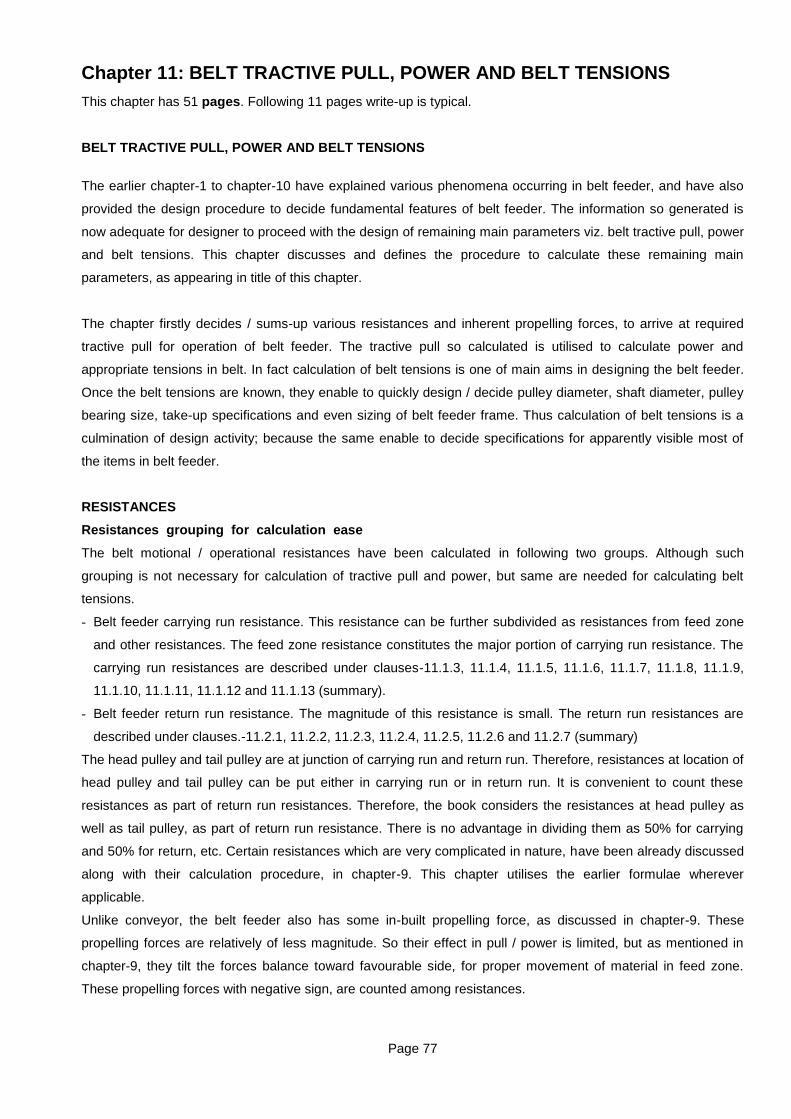
Page 77
Chapter 11: BELT TRACTIVE PULL, POWER AND BELT TENSIONS
This chapter has 51 pages. Following 11 pages write-up is typical.
BELT TRACTIVE PULL, POWER AND BELT TENSIONS
The earlier chapter-1 to chapter-10 have explained various phenomena occurring in belt feeder, and have also
provided the design procedure to decide fundamental features of belt feeder. The information so generated is
now adequate for designer to proceed with the design of remaining main parameters viz. belt tractive pull, power
and belt tensions. This chapter discusses and defines the procedure to calculate these remaining main
parameters, as appearing in title of this chapter.
The chapter firstly decides / sums-up various resistances and inherent propelling forces, to arrive at required
tractive pull for operation of belt feeder. The tractive pull so calculated is utilised to calculate power and
appropriate tensions in belt. In fact calculation of belt tensions is one of main aims in designing the belt feeder.
Once the belt tensions are known, they enable to quickly design / decide pulley diameter, shaft diameter, pulley
bearing size, take-up specifications and even sizing of belt feeder frame. Thus calculation of belt tensions is a
culmination of design activity; because the same enable to decide specifications for apparently visible most of
the items in belt feeder.
RESISTANCES
Resistances grouping for calculation ease
The belt motional / operational resistances have been calculated in following two groups. Although such
grouping is not necessary for calculation of tractive pull and power, but same are needed for calculating belt
tensions.
- Belt feeder carrying run resistance. This resistance can be further subdivided as resistances from feed zone
and other resistances. The feed zone resistance constitutes the major portion of carrying run resistance. The
carrying run resistances are described under clauses-11.1.3, 11.1.4, 11.1.5, 11.1.6, 11.1.7, 11.1.8, 11.1.9,
11.1.10, 11.1.11, 11.1.12 and 11.1.13 (summary).
- Belt feeder return run resistance. The magnitude of this resistance is small. The return run resistances are
described under clauses.-11.2.1, 11.2.2, 11.2.3, 11.2.4, 11.2.5, 11.2.6 and 11.2.7 (summary)
The head pulley and tail pulley are at junction of carrying run and return run. Therefore, resistances at location of
head pulley and tail pulley can be put either in carrying run or in return run. It is convenient to count these
resistances as part of return run resistances. Therefore, the book considers the resistances at head pulley as
well as tail pulley, as part of return run resistance. There is no advantage in dividing them as 50% for carrying
and 50% for return, etc. Certain resistances which are very complicated in nature, have been already discussed
along with their calculation procedure, in chapter-9. This chapter utilises the earlier formulae wherever
applicable.
Unlike conveyor, the belt feeder also has some in-built propelling force, as discussed in chapter-9. These
propelling forces are relatively of less magnitude. So their effect in pull / power is limited, but as mentioned in
chapter-9, they tilt the forces balance toward favourable side, for proper movement of material in feed zone.
These propelling forces with negative sign, are counted among resistances.
Page 78
The other crucial point is the implication of actual shear plane on resistances within feed zone. The designer has
two options, viz.
1. Just consider shear at interface and calculate resistances accordingly.
2. Decide theoretical shear plane as per chapter - 9 and make calculations for resistances based on this shear
plane.
In case of first option, i.e. calculation made by assuming shear at interface, would have relative merit / demerit in
comparison to actual conditions, as below.
Situation-1: The material is actually shearing at interface, and we are also calculating resistances considering
material shear at interface. So no compromise in calculations.
Situation-2: The material shear is on plane, which is intersecting on back plate, as shown in figure-9c, page-285,
chapter-9. In this situation, the overall net resistance (sum of shear resistance, skirt plates resistances, skirt
plate reaction pushing force and pushing force on upper face) will be somewhat less than net resistance
attributed to same items based on shear at interface. So, calculations will be on safer side, by reasonable
magnitude most of the time. For this situation-2, the designer can safely opt for calculation based on shear at
interface (i.e. situation-1).
Situation-3: The material shear is on plane which is intersecting belt, within feed zone, as shown in figure-9d,
page-288, chapter-9. In this situation, net resistance (due to shear resistance, skirt plates resistances, skirt
plates reaction pushing force and pushing force on upper face) will be less (by sufficient margin say up to 10%)
than net resistance attributed to same items based on shear at interface. However, the shear along actual plane
introduces one new / additional resistance directly to belt i.e. material rubbing on belt or material shear
immediately above belt level, in portion rear of triangle tail. This would jack up the comparative value of
resistance associated with actual shear plane. It appears that even in this situation-3, there would be tolerable
difference between two results (i.e. calculation basis shear at interface versus calculation basis shear on actual
plane). However, it is difficult to predict in a very specific way. So, calculation procedure (formulae) have been
given for both the options. The situation-3 is mostly relevant to uniform cross section skirt board and long feed
zone, where resistance based on actual shear plane, can need attention.
All resistances under this cl.-11.1.0 and its sub-clauses are for steady state operation (dynamic condition). This
also means C2 value corresponds to material pressure at hopper outlet during flow condition.
The resistance during start-up phase is discussed under cl.-11.4.1 (11.4.0). This affects only few values /
parameters of steady state resistance.
Carrying run resistance Rc summary Rsh : Material shear resistance
Rsk1 : Skirt plates resistance, feed zone
Rsk2 : Skirt plates resistance, beyond feed zone
Rsk3 : Skirt rubber to belt resistance
Rcc : Conveying resistance
Rslc : Slope resistance
Rpi : Force from interface
Rpb : Force from skirt board back plate
Rps : Force from skirt plates

Page 79
The algebraic sum of above resistances, is the resistance Rc from carrying run, during operating, steady state.
Return run resistance summary, Rr
Rcr : Conveying resistance, return run
Rslr : Slope resistance, return run
Rce : External belt cleaner resistance
Rci : Internal belt cleaner resistance
Rw : Belt wrap resistance around pulleys
Rt : Pulley turning resistance
The algebraic sum of above resistance, is the resistance from return run during operation, steady state.
Example -1
Calculate belt feeder tractive pull (during steady state), power (this is always for steady state), motor kW, belt
tractive pull during starting and starting phase total time ts, Motor starting is DOL, without fluid coupling. The
1400 mm belt feeder particulars are as below (this is same as example-6, chapter-9, page-282).
he = 0.82 m, hi = 0.27 m, He = 0.938 x 3 = 2.81m, Hi = 0.4 x 3 = 1.2 m, We = 0.938 m
Wi = 0.4m, = 5.710593°, Ge = 0.1, = 2.8°, Gp = 0.0489, L = 5.5 m,
= 2°, C2 = 3, = 36°, s = 0.423, Qd = 480 mtph, b = m = 0.6346, = 1000 kg/m3
Belt velocity V = 0.23 mps, L1 = 10 m, L2 = 6.25 m, Lsk = 3.5 m, h = 0.62 m
Mb = 30 kg/m, Mc = 150 kg/m, f = 0.04 Mr = 15 kg/m
The C2 value during static status is 2.3, a case similar to rotary wagon tippler with steep hopper. The belt feeder
is handling granular material. Select the drive as if with induction motor.
This belt feeder has been already checked for its shear plane (page-283 to 284). Accordingly, the material shear
is at interface. Therefore, following calculations for tractive pull and power are on the basis of material shear at
interface (situation-1).
Solution :
Material shear resistance Rsh
Me = 7752 kg
Gravity force F = Me . g = 7752 x 9.81 = 76047 N
Rsh = m . F . [cos( + )] . cos = 0.6346 x 76047 x [cos 7.710593] x cos 5.710593 = 47586 N
Skirt plate resistance Rsk1, feed zone
Rsk1 = 0.25 s . K . . g . L . (2 he - Ge . L) . (2 . he + 4 C2 . We - Ge . L - 4 . C2 . Gp . L) N
K = (1 -sin 36) (1 + sin 36) = 0.2596
Rsk1 = 0.25 x 0.423 x 0.2596 x 1000 x 9.81 x 5.5 x (2 x 0.82 - 0.1 x 5.5) x (2 x 0.82 + 4 x 3 x 0.938 - 0.1 x 5.5 - 4
x 3 x 0.0489 x 5.5) = 14722 N
Skirt plates resistance Rsk2, beyond feed zone
Rsk2 = s . K . . g . h2 . Lsk N
Rsk2 = 0.423 x 0.2596 x 1000 x 9.81 x 0.622 x 3.5 = 1449 N
222
2222
5.5x0489.0x3
45.5x938.0x0489.0x2938.0x
710593.5cos
5.5x710593.7cosx3x1000
kgL.Gp.3
4L.We.Gp.2We.
cos
L.cos.C.Me

Page 80
Skirt rubber to belt resistance, Rsk3
Rsk3 = 90 x 9 = 810 N
Conveying resistance carrying run, Rcc
Ms = . [6 he . We . L - 3 (Ge . We + 2 Gp . he) . L2 + 4 Ge . Gp . L
3] 6 kg
= 1000 x [6 x 0.82 x 0.938 x 5.5 - 3 x (0.1 x 0.938 + 2 x 0.0489 x 0.82) x 5.52 + 4 x 0.1 x 0.0489 x 5.5
3] 6
Ms = 2141 Kg
Me = 7752 kg (as calculated for material shear resistance Rsh, in the beginning of the solution)
Mm = Qd (3.6 V) = 480 (3.6 x 0.23) = 579.7 kg/m
Rcc = [Ms + Me + Mb . L1 + Mc . L1 + Mm (L1 - L - 0.5)] . f . g N
= [2141 + 7752 + 30 x 10 + 150 x 10 + 579.7 x (10 - 5.5 - 0.5)] x 0.04 x 9.81
Rcc = 5498 N
Slope resistance carrying run, Rslc
Rslc = Mb . L1 . g . sin + Mm . L2 . g . sin N
= 30 x 10 x 9.81 x sin 2 + 579.7 x 6.25 x 9.81 x sin 2 = 1343 N
The force from interface, Rpi
F = Me. g
Me = 7752 kg (as calculated for material shear resistance Rsh, in the beginning of the solution)
F = 7752 x 9.81 = 76047 N
Rpi = - F. [cos( + )] . sin N
= - 76047 x [cos (7.710593)] x sin 5.710593 = -7498 N
Force from back plate, Rpb
Rpb = - 0.25 . K . . g . hi . Wi . (hi + 2 . C2 . Wi) N
= - 0.25 x 0.2596 x 1000 x 9.81 x 0.27 x 0.4 x (0.27 + 2 x 3 x 0.4) = -183 N
Force from skirt plates, Rps
Rps = - 0.25 K . . g . L . (2 he - Ge . L) . (2 . he + 4 C2 . We - Ge . L - 4 . C2 . Gp . L) . sin N
= - 0.25 x 0.2596 x 1000 x 9.81 x 5.5 x (2 x 0.82 - 0.1 x 5.5) x (2 x 0.82 + 4 x 3 x 0.938 - 0.1 x 5.5 - 4 x 3 x
0.0489 x 5.5) x sin 2.8
= - 1700 N
Carrying run resistance Rc summary
Rsh = 47586 N
Rsk1 = 14722 N
Rsk2 = 1449 N
Rsk3 = 810 N
Rcc = 5498 N
Rslc = 1343 N
Rpi = -7498 N
Rpb = -183 N
Rps = -1700 N
Total = 62027 N This is total resistance of carrying run.
Conveying resistance, return run, Rcr
Rcr = f . g . L1 . (Mb + Mr) = 0.04 x 9.81 x 10 x (30 + 15) = 177 N
Slope resistance, return run, Rslr
Page 81
Rslr = - Mb . L1 . g . sin = - 30 x 10 x 9.81 x sin 2 = -103 N
External belt cleaner resistance, Rce
The input data are, e = 0.6, Ae = 0.0448 m2, Pe = 50000 N/m
2
Rce = e . Ae . Pe = 0.6 x 0.0448 x 50000 = 1344 N
Internal belt cleaner resistance
The input data are, i = 0.6, Ai = 0.0336 m2, Pi = 50000 N/m
2
Rci = i . Ai . Pi = 0.6 x 0.0336 x 50000 = 1008 N
Belt wrap resistance around pulleys, Rw
The calculation of wrap resistance and pulley turning resistance requires belt tensions, pulley diameter, shaft
diameter at bearings, which are not known at this stage. Actually this exercise is to find these values. So,
presently, sum up all resistances without Rw and Rt.
All resistances (without Rw and Rt) = 62027 + 177 -103 + 1344 + 1008 = 64453 N
Make approximate (or actual) design using this value of resistance and decide tension, pulley diameter and shaft
diameter at bearings.
Here approximate method is followed as an additional information to reader. Consider drive factor 0.5, T1 = 1.5 x
64453 = 96679 N, T2 =0.5 x 64453= 32226 N.
At this stage consider both the values approximately 10% more. The values of Rw and Rt are small, and such
consideration does not make much difference in total resistance. Accordingly,
Fb1 = 0.5 (T1 + T2) = 0.5 ( 1.1 x 96679 + 1.1 x 32226) = 70898 N
Fb2 = 1.1 x 32226 = 35449 N
Also, tentative belt could be 1400 mm EP 800 / 4, covers 10 & 5 mm, grade M24. This belt total thickness is
approximately 20 mm. Pulley diameters are (650 + 2x12 RL) mm, (500 + 2x10 RL) mm and (400 +2x10 RL) mm.
The shaft diameters at bearings are likely to be 150 mm and 120 mm tentative. After making final design these
resistances are recalculated, along with their implication on total resistance (which would be of small
magnitude). That is to say first stage design output will become input to final design.
The input data for this calculation are :
t = 20 mm, Fb1 = 70898 N, Fb2 = 35449 N, N2 = 2, Textile fabric belt.
Rw = 623 N
Pulley turning resistance, Rt
Rt = 0.005 x (2 . Fb2) x d2 x N2 D2 = 0.005 x (2 x 35449) x 120 x 2 520 = 163 N
Return run resistance summary, Rr
Rr = Rcr + Rslr + Rce + Rci + Rw + Rt = 177 - 103 + 1344 + 1008 + 623 + 163 = 3212 N
Rf = Rc + Rr = 62027 + 3212 = 65239 N
Power at drive pulley periphery, pk1 = P . V 1000 = 65239 x 0.23 1000 = 15 kW
Power required at motor shaft, pk2 = pk1 = 15 0.9 = 16.67 kW (considering dive efficiency 90%)
Belt feeder torque at drive pulley rim, steady settled speed = P . D1 (1000 x 2) = 65239 x 674 (1000 x 2) =
21985 Nm
5202x1400
35449x10140x20x1400x009.0674
1400
70898x10140x20x1400x009.0
DN.B
2Fb10140.t.B009.0D
B
1Fb10140.t.B009.0Rw 221

Page 82
Belt feeder torque TQm at motor shaft, steady settled speed = 21985 (.i) Nm = 21985 (0.9 x 112)
=218.1Nm, drive efficiency and gear box ratio as mentioned below.
Drive selection.
The drive pulley diameter is 650 + 2 x 12 = 674 mm, as mentioned above. The drive system total speed
reduction would be i = 112 based on 720 rpm motor and 674 mm diameter drive pulley, to get belt speed of
nearly 0.23 mps. The totally enclosed gear box along with flexible coupling at input shaft and flexible coupling at
output shaft, have been considered for total speed reduction ratio of 112. One can also use geared motor, if
same is available with electrical motor of required specifications. This would eliminate input coupling.
Starting state :
Here C2 static is less than C2 dynamic. Hence Rfsw 1.6 Rf.
Rfsw = 1.6 x 65239 = 104382 N
Therefore required starting torque at feeder shaft = 104382 x (0.5 x0.674) = 35176 Nm.
Required starting torque at motor shaft = 35176 (112 x 0.9) = 348.9 Nm
Choose the drive motor which has stalled (zero speed) torque and pull-up torque at least 30% more than the
above value 348.9 Nm
Chosen motor say 22.4 kW
This motors rated torque = 22.4 x 9555 720 = 297.26 Nm
This is greater than the required steady speed torque
This motor pull-up torque and stalled (zero speed) torque should be ≥ 297.26 x 1.3 = 387 Nm. It seems the
regularly available motor will have stalled torque and pull-up torque suitable for this. Nema-C type motor can
have it as high as 75%, although it is not necessary to have such a torque.
TAKE-UP
Belt feeder includes take-up device to maintain proper tension in belt. The „proper‟ tension implies „minimum‟
tension to fulfill all the functional needs such as:-
- Adequate tension to transmit mechanical power from drive pulley to belt in all operating conditions, by well
known relation T1 / T2 e
- Adequate tension to limit sag of belt between idlers, within allowable limit so that material leakage between
belt and skirt board is of acceptable level such that it does not spill from belt, but gets conveyed for discharge
at head pulley.
If the tension is more than the necessary, it will result in costlier belt, pulleys and terminal structures. So, the
designer always decides minimum tension to suit above requirements. Constructionally 3 types of take-ups viz.
screw take-up (plain), screw take-up with hydraulic tensioner and horizontal gravity take-up at tail end can be
used. Functionally, these take-up devices can be grouped in two types viz. `fixed take-up pulley type‟ and
`floating take-up pulley type‟. The reader may wonder with the mention of gravity take-up at tail end, but this has
been discussed for possibility of its use in context of modern day high capacity and heavy-duty belt feeders.
Take-up types
Following is the information about the different types take-up, applicable to belt feeders:

Page 83
Screw take-up (simple)
Simple screw take-up suits very well to light-duty belt feeders. This is the most economical type of take-up
device because it is simple mechanism and is extensively used. The take-up device is shown in figure-11F and
figure-11G, and is generally installed with tail pulley, which also acts as take-up pulley.
The device includes 2 numbers of take-up screw with nut in suitable form. In one arrangement screw remains at
same location, and turning of the screw shifts nut. The take-up pulley plummer block is mounted on guide which
is attached to the nut. The nut movement carries pulley with it for tightening the belt. Such screw-nut are
mounted under angle-frame for protection against spilled material; and therefore are known as protected screw
take-up device. The advantage of such take-up device is the use of standard plummer block for pulley support,
and protection of screw-nut from spilled material, and suitability for installation on regular tail terminal.
The other arrangement includes shifting screw. The turning of nut shifts the screw. The screw end is connected
with special shaped plummer block moving in guides. Such arrangement has screws and pulley centre-line in
same plane for transfer of belt force to screw without tilting-movement. Thus the arrangement is more robust
from design consideration. However it requires special type of plummer block which increases the inventory.
In the aforesaid arrangements, both side screws are operated alternatively in short step movement. The belt
tightening is by judgement according to skill of the maintenance personnel. Such screw take-ups with manual
tightening are commonly used for average duty feeders, in consideration to economy and simplicity. The author
does not recommend use of such take-up for heavy or important class belt feeder where specific tension is must
for proper functioning of belt feeder. The specific tension can not be achieved by manual judgement.
Screw take-up with hydraulic tensioner
The screw take-up device with hydraulic tensioner is recommended for medium to heavy class feeders. In this
arrangement, portable cylinder piston assembly is attached between pulley-guide-block and conveyer structure,
at each side. The nuts (or holding devices) are loosened to permit free movement of guide-blocks. Hydraulic
hand-pump (simultaneous action to both cylinders) is used to generate necessary oil pressure for desired take-
up force. The pulley shifts to new position by hydraulic thrust, where it is locked by nuts on screws.
Subsequently, the hydraulic attachments are removed. Such hydraulic tensioner device is in effect a
maintenance device / tool. This type of take-up feature can mostly fit to arrangement similar to figure-11G or its
appropriate modification.
The other alternative option is to have load cells appropriately placed at tail end, and use their reading while
tightening the take-up screw (of earlier title).
turn screwProvision to
Full threaded
Nut suitably connectedto guide block
Figure-11F (Schematic)
screw
Pulley
Nut with provision
Figure-11G (Schematic)
for turning
Pulley

Page 84
All the screw take-up devices are functionally `constant belt length take-up‟ i.e. take-up pulley does not shift
during feeder operation. This means belt length remains constant whether the feeder is running at steady
speed, starting or stoppage.
Screw take-up creates tension in belt by stretching the belt. The belt elongates after certain use, which results
into reduced tension. This would require stretching (i.e. re-tightening) to restore the tension. The belt needs
periodic re-tightening to maintain same value of tension. The new belt needs tightening after short time use, but
subsequently such necessity arises after prolonged time interval. The belt has two types of stretches viz.
permanent elongation and elastic elongation. The periodic resetting arises due to permanent elongation which is
more initially but it diminishes with time.
Horizontal gravity take-up
As of now this arrangement has been rarely used for belt feeder. Because in general the importance / necessity
for presence of appropriate tension in belt feeder, has not received adequate attention (as an average situation).
The usual difficulty associated with belt feeder such as material leakage, etc. are consequence of improper
tension instead of just focussing on peripheral issues. The advantages of the gravity take-up are: (1) It provides
assured value of take-up force at all the times. (2) The take-up device is maintenance free to apply needed
force. (3) Take-up force is not effected by belt stretch (within the operating stroke). Also, thermal expansion /
contraction of belt does not effect tension. This is due to floating nature of take-up pulley.
The disadvantages of such take-up are: (1) If the belt snaps, the sliding unit and counter weight will hit the
barrier. (2) The slackening of belt is difficult compared to non-gravity take-up. (3) It needs more space and
special precaution to make it hazard-free for the belt feeder installation, which is often in a constrained space
unlike conveyor.
The designer to choose the type of take-up appropriate to the application. Simple screw take-up to be used
where it can suit, and general tendency for same to be restricted. The screw take-up with hydraulic tensioner or
load cell, will have satisfactory performance, but needs periodic checking and resetting for restoration of belt
tension. As against this, gravity take-up will attend itself for the tension, but required space for its installation and
to make it hazard-free is to be examined by designer.
Figure-11H
Covering
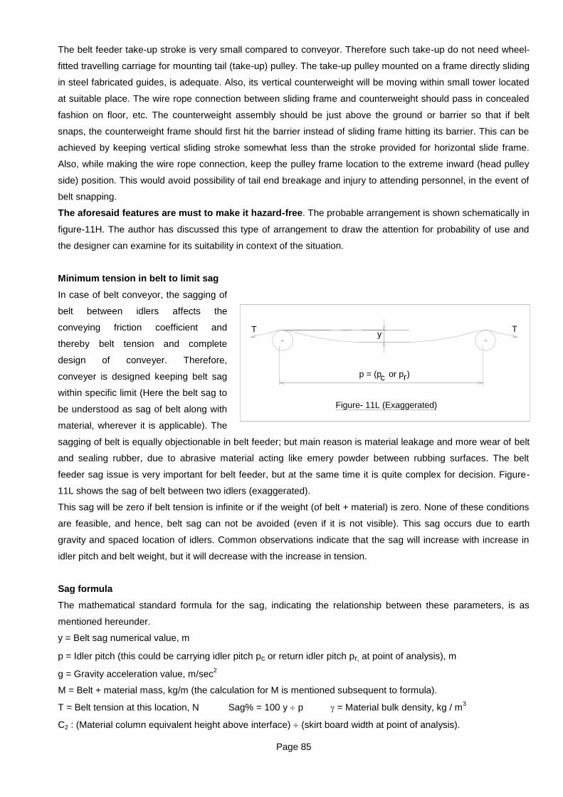
Page 85
The belt feeder take-up stroke is very small compared to conveyor. Therefore such take-up do not need wheel-
fitted travelling carriage for mounting tail (take-up) pulley. The take-up pulley mounted on a frame directly sliding
in steel fabricated guides, is adequate. Also, its vertical counterweight will be moving within small tower located
at suitable place. The wire rope connection between sliding frame and counterweight should pass in concealed
fashion on floor, etc. The counterweight assembly should be just above the ground or barrier so that if belt
snaps, the counterweight frame should first hit the barrier instead of sliding frame hitting its barrier. This can be
achieved by keeping vertical sliding stroke somewhat less than the stroke provided for horizontal slide frame.
Also, while making the wire rope connection, keep the pulley frame location to the extreme inward (head pulley
side) position. This would avoid possibility of tail end breakage and injury to attending personnel, in the event of
belt snapping.
The aforesaid features are must to make it hazard-free. The probable arrangement is shown schematically in
figure-11H. The author has discussed this type of arrangement to draw the attention for probability of use and
the designer can examine for its suitability in context of the situation.
Minimum tension in belt to limit sag
In case of belt conveyor, the sagging of
belt between idlers affects the
conveying friction coefficient and
thereby belt tension and complete
design of conveyer. Therefore,
conveyer is designed keeping belt sag
within specific limit (Here the belt sag to
be understood as sag of belt along with
material, wherever it is applicable). The
sagging of belt is equally objectionable in belt feeder; but main reason is material leakage and more wear of belt
and sealing rubber, due to abrasive material acting like emery powder between rubbing surfaces. The belt
feeder sag issue is very important for belt feeder, but at the same time it is quite complex for decision. Figure-
11L shows the sag of belt between two idlers (exaggerated).
This sag will be zero if belt tension is infinite or if the weight (of belt + material) is zero. None of these conditions
are feasible, and hence, belt sag can not be avoided (even if it is not visible). This sag occurs due to earth
gravity and spaced location of idlers. Common observations indicate that the sag will increase with increase in
idler pitch and belt weight, but it will decrease with the increase in tension.
Sag formula
The mathematical standard formula for the sag, indicating the relationship between these parameters, is as
mentioned hereunder.
y = Belt sag numerical value, m
p = Idler pitch (this could be carrying idler pitch pc or return idler pitch pr, at point of analysis), m
g = Gravity acceleration value, m/sec2
M = Belt + material mass, kg/m (the calculation for M is mentioned subsequent to formula).
T = Belt tension at this location, N Sag% = 100 y p = Material bulk density, kg / m3
C2 : (Material column equivalent height above interface) (skirt board width at point of analysis).
p = (p or p
yT
Figure- 11L (Exaggerated)
c )r
T
Page 86
Qd = Design capacity, mtph V = Belt speed, mps (also small v)
Mb = Belt mass, kg/ m Ge = Skirt board elevation gradient, Ge = tan
Gp = Skirt board gradient in plan, Gp = tan
T = 12.5 M . g . p (sag %) N Alternatively, (sag%) = 12.5 M . g . p T
The first formula can be used to decide required tension from selected value of sag%.
The alternative formula can be used to decide sag % that would occur for known value of tension.
The value of M to be used in this equation is as below:
For portion beyond feed zone
Generally the belt tension will be comparatively more, and the value of M will be less in this zone, compared to
feed zone. Hence, this calculation will show idler pitch more than feed zone, but it is beneficial to keep it less,
say within 325 mm..
Mm = Qd (3.6 v) kg/ m, this is material mass per metre.
M = Mm + Mb kg/m
For feed zone portion
Suppose belt sag condition is to be analysed at a distance x from exit end.
Skirt board width, W1 at that point = We - 2 Gp . x
Skirt board height, h1 at that point = he - Ge . x
Material column equivalent height at H1 = C2 . W1
M = . W1 . (h1 + H1) x 1 +Mb = . W1 . (h1 + H1) +Mb = . W1 . h1 + . C2 . W12 + Mb kg/ m
For return run
For return run this is simply belt mass kg/m. Hence M = Mb kg/m.
Magnitude of Sag
The sag value is simply 1 % for return run. The carrying run has to hold material from feed zone to discharge
pulley, but material at feed zone is under more pressure. Therefore, sag value (numerical value in mm) selected
for feed zone is also used for portion beyond feed zone. The sag value for feed zone is discussed here, and it
relates to following issues.
- The locations (or points), which are to be chosen for sag analysis.
- The allowable sag at these locations (or points).
For the belt feeder of expanding cross section, the M value increases as we advance from rear side to exit side
of feed zone. But belt tension also increases as we advance towards exit side of feed zone. If the skirt board
expansion gradients Ge and Gp are sufficiently large, the feed zone exit end condition would be mostly
governing. However, if these gradients are not adequate, then the situation at rear end could be governing. For
the skirt board of uniform cross section, the sag condition at the rear end of feed zone would be governing
(worst). The designer is to see the acceptability of leakage gap at both the ends, possibly for a compromise
decision. After all, aggregate leakage from entire feed zone matters, and not the leakage at critical or worst
point.
The allowable sag depends upon fineness of material, feed zone length, material pressure and also to some
extent abrasiveness of the material as below:
- The leakage is more for finer material, i.e. allowable sag will be comparatively less for finer material.

Page 87
- The leakage material is to be accommodated by belt, prior to its spillage. This material increases with feed
zone length. Thus comparatively less sag is to be considered for longer length of feed zone.
- The material under high pressure would tend to force its way through gap. So comparatively less sag is
preferred, when dealing with deep hopper imposing high pressure of material
- Comparatively less sag would be better for more abrasive material.
- Comparatively less sag for narrow belt, which has less margin at belt edge to hold material.
The sag value to be chosen is subjective. The designer can use his experience in dealing with different types of
materials. The sag % value is directly linked to idler pitch. For the belt feeder, it is the numerical value of sag
(mm) that matters and not the sag %.
Again the sag value is to be correlated with the actual gap (maximum at centre of pitch distance). The belt sag
profile vary up-down continuously during operation, in tune with variation in vertical force (i.e. variation in level of
material in hopper). This prevents creation of zero gap between skirt rubber and belt, even though skirt rubber
tends to acquire it by its wear. The actual gap between skirt rubber and belt can be considered about 75% of sag
value used in calculation. Thus for example, if idler pitch is 250 mm and sag is 1%, then the gap is likely to be
2.5 x 0.75 = 1.875 mm. The designer is to see the acceptability of the gap so calculated. The foregoing
information / explanation helps to understand the applicable technical issues. The author suggests to adopt
following approach for technical calculation and decision:
- For usual belt feeder, avoid using pitch more than 250 mm under feed zone, even if sag (gap) condition
allows it to be more. The improved performance from this would be more than additional cost of few idlers.
- If need be, use the idler pitch closest to roller diameter, just keeping about 20 to 25 mm gap between rollers.
The calculation for belt feeder under high pressure can often lead to such requirement. If the rollers are
mounted on idler frame; the frame base to be formed by angle piece welded at transom end, instead of base
plate under transom. This would avoid base length greater than roller diameter.
- In general, belt feeder does not deal with very large lumps, continuously falling from great height. So, roller
diameter less than 200 mm and closer pitch could be possible, when needed. If the closer pitch is not
possible and material pressure is high; then higher tension in belt would be required. This means costlier
belt, pulleys, bearings and drive.
- In a heavy class belt feeder, vertical force on belt can be tonnef / metre rather than kgf / m, under feed zone.
The rolling support provides wear free surface to the belt.
It seems that the actual gap of 5 mm between skirt rubber and belt can be used depending upon the material,
belt width, feed zone length and belt feeder length. If the idler pitch is 200 mm, then the above implies 2.5% sag.
If the idler pitch is 250 mm, then above implies sag value of 2%. This is just a typical method for calculation.
Some time it could be very expensive to restrict actual gap of 5 mm. In such circumstances, the designer can
use higher value, say up to 6 to 10 mm, judging the need/ suitability for application. This implies 3% and 4% sag
with respect to 200 mm pitch idler. The lesser magnitude of sag is better because it implies less leakage
between skirt rubber and belt.
Chapter 13: TRANSITION DISTANCE
This chapter has 5 pages. Following 5 pages write-up is typical.
TRANSITION DISTANCE
The belt feeder carrying run will be of troughed type, if the belt feeder is equipped with picking type idler or 3-roll

Page 88
troughing idlers. In such belt feeder; the belt is flat when on pulley, but it acquires trough shape when being on
idler. The change of profile from flat to trough OR trough to flat results into additional strain / stress in belt. The
change of this profile is done gradually so that additional stress strain remains within tolerable / allowable limit, to
prevent damage to belt and also to have workable belt feeder. In effect, this requires certain minimum distance
along feeder, for transformation of belt from flat to trough (or trough to flat), safely without damage to belt
carcass. This chapter describes the design procedure to calculate this minimum distance which is called
„minimum transition distance‟. Fifure-13A shows the belt profile in transition zone. The transition distance being
used should be greater than or equal to this „minimum transition distance‟.
Generally, the transition distance used is near to minimum, because excess distance can have disadvantages
such as (1) Increase in centre to centre length of belt feeder. (2) Difficulty to accommodate within available
space. (3) Longer length of special shape skirt-edges (for 3-equal roll trough idlers) matching to transition
distance, at discharge end.
The designer can always use transition distance more than minimum if layout and available space permit the
same. The transition distance issue is more severe in case of belt conveyors, due to deep troughing angles. The
belt feeders troughing angles are comparatively less, and thereby would pose less difficulty in providing the
required transition distance. This chapter is not applicable to flat belt feeder.
BELT STRESS - STRAIN AND BEHAVIOUR IN TRANSITION ZONE
Figure-13A shows the transition zone.
The figure shows pulley top point
location raised up by distance h,
compared to the line touching the top of
central rollers in this zone (reference
level of belt). The belt rise h is shown in
figure, because it is part of standard
(comprehensive) formula applicable to
conveyors as well as belt feeders. However, the belt rise does not suit belt feeder (if there is feeding in transition
zone) and it should be taken zero or almost zero. As can be seen in this figure, the geometric dimension FG is
larger than Ly (or FJ). The belt same segment when not on transition zone, will have FG = Ly. This implies the
belt outward portion (towards edges) is getting stretched accompanied by reduction in safety factor in this part of
the belt. This is shown in figure-13B.
In reality, the belt segment has to create dimensional difference between edges and central portion, when it is
forced to pass through transition zone. The edge stretch also creates compressive load (stress) in middle
portion, along X and Y directions due to force reaction in the carcass. The belt was under uniform longitudinal
tensile stress before transition zone. However when it is passing through transition zone, the side portions are
subjected to elongation strain at edges, which adds in to earlier tensile stress. The belt middle portion was also
under identical tensile stress, but now it gets superimposed by compressive stress. So, the middle portion will
have effective tensile stress less than the original, as far as longitudinal direction is concerned. In addition, belt is
also subjected to compressive stress along transverse direction due to belt tendency to slide down on side
rollers due to bow - string effect. The situation will result into belt buckling in middle portion of segment i.e. belt
fold-up (or fold-up tendency) will appear in this zone, if transition distance is not adequate in relation to prevailing
h
F
Figure-13 A
G
J
Ly

Page 89
tensions in the belt. Thus, transition distance depends upon carcass particulars and prevailing tensions in the
belt. The transition distance should be sufficiently large so that :
- Belt edges stretching should not cross the allowable limit (lower than yield condition, by adequate margin
during life of belt).
- Belt central portion should not buckle or fold-up (lower than fold-up limiting value by adequate margin during
life of belt).
The calculations for required transition distance cannot be done purely on theoretical basis. This requires
extensive testing for three-dimensional behaviour of „hollow‟ belt, which can best be done by belt manufacturer
who will have very large number of samples as needed for such tests. The design procedure has been
reproduced here from Author‟s book “Engineering Science and Application Design for Belt Conveyors”, which is
on the basis of published data of M/s ContiTech Germany, with their kind permission for the said book. One can
also refer to the article by D Beckmann and Rainer Alles on this subject.
NOMENCLATURE
B: Belt width, mm
bf: Belt portion length on side roller, mm (refer figure-13C)
: Troughing angle, degree (refer figure-13C).
Tx: Belt tension in N, at point of analysis, steady state
Txm: Belt tension in N, at point of analysis, momentary state
Tuj: Belt joint unit strength, N/mm (This is equal to nominal unit strength x joint efficiency. For example
EP800 with joint efficiency 0.75, Tuj = 800 x 0.75 = 600 N/mm)
E
F
H
G F
E
G
H
Width
Belt segment shape before transition zone Belt same segment shape when in transition zone(ignoring compensation)
Figure-13 B (schematic for understanding)
X - '
X X +
Ly
h
Figure-13 C
Pulley
h
bf

Page 90
B
Tx
Tuj Sx analysis, ofpoint at factor safety existing stateSteady :Sx
B
Txm
Tuj Sxm analysis, ofpoint at factor safety existing stateMomentary :Sxm
Sp: Permitted bare minimum safety factor, steady state (continuous operation)
Spm: Permitted bare minimum safety factor, momentary state.
The values of Sp and Spm are as below:
Sp Spm
Fabric belt 3.6 3.0
Steel cord belt, 1 or 2 lap splice 3.0 2.5
Steel cord belt, 3 or more lap slice 3.3 2.8
KG: Belt characteristic parameter. The values are as per table-27 refer book.
h: Pulley rise relative to central roller, mm. Generally one should opt for h = 0, for belt feeder.
Ly: Transition length, mm
Lyc: Transition length including compensation effect, mm
TRANSITION LENGTH (MINIMUM)
The transition length from flat to trough or trough to flat can be calculated as below. The required transition
length is to be calculated for steady state and alternatively for momentary state; and use one which is more.
Additional nomenclatures are as below.
The formulae can use mm or m. The answer will be in the unit so selected.
The value of h (if used) should not exceed following limiting condition for proper functioning. This is just
mentioned as a part of standard formula for conveyors as well as feeders.
h = (1 – cos . bf sin . Preferably, h should be limited up to 15% of bf . sin, and concave curvature
zone of belt from pulley should not exceed last idler in transition zone to avoid interference with skirt board (if
same is immediately after transition zone).
Steady state requirement
Firstly, find out value of fconvex for steady state.
If Sx fconvex, then only edge elongation is governing.
B
b
S f
f
p
convex
mmK . K . Sp -Sx
Sp .Sx .
b
h -
57.3 . B Ly 1G
f
3
f2
3
f
2
f1
B
b K and
B
b -
B
b K
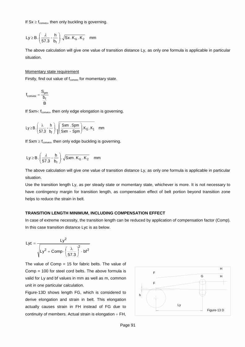
Page 91
If Sx fconvex, then only buckling is governing.
The above calculation will give one value of transition distance Ly, as only one formula is applicable in particular
situation.
Momentary state requirement
Firstly, find out value of fconvex for momentary state.
If Sxm fconvex, then only edge elongation is governing.
If Sxm fconvex, then only edge buckling is governing.
The above calculation will give one value of transition distance Ly, as only one formula is applicable in particular
situation.
Use the transition length Ly, as per steady state or momentary state, whichever is more. It is not necessary to
have contingency margin for transition length, as compensation effect of belt portion beyond transition zone
helps to reduce the strain in belt.
TRANSITION LENGTH MINIMUM, INCLUDING COMPENSATION EFFECT
In case of extreme necessity, the transition length can be reduced by application of compensation factor (Comp).
In this case transition distance Lyc is as below.
The value of Comp = 15 for fabric belts. The value of
Comp = 100 for steel cord belts. The above formula is
valid for Ly and bf values in mm as well as m, common
unit in one particular calculation.
Figure-13D shows length FG, which is considered to
derive elongation and strain in belt. This elongation
actually causes strain in FH instead of FG due to
continuity of members. Actual strain is elongation FH,
mmK . K .Sx . b
h -
57.3 . B Ly 2G
f
mmK . K . Spm - Sxm
Spm . Sxm .
b
h -
57.3 . B Ly 1G
f
mmK . K . Sxm . b
h -
57.3 . B Ly 2G
f
B
b
S f
f
pmconvex
22
2
2
bf3.57
CompLy
LyLyc
F
Figure-13 D
h
G HF
H
Ly
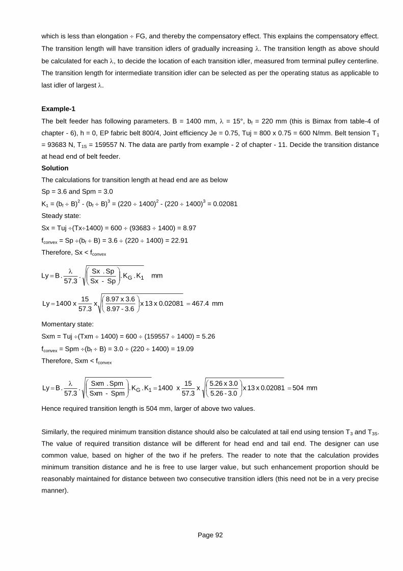
Page 92
which is less than elongation FG, and thereby the compensatory effect. This explains the compensatory effect.
The transition length will have transition idlers of gradually increasing . The transition length as above should
be calculated for each , to decide the location of each transition idler, measured from terminal pulley centerline.
The transition length for intermediate transition idler can be selected as per the operating status as applicable to
last idler of largest .
Example-1
The belt feeder has following parameters. B = 1400 mm, = 15°, bf = 220 mm (this is Bimax from table-4 of
chapter - 6), h = 0, EP fabric belt 800/4, Joint efficiency Je = 0.75, Tuj = 800 x 0.75 = 600 N/mm. Belt tension T1
= 93683 N, T1S = 159557 N. The data are partly from example - 2 of chapter - 11. Decide the transition distance
at head end of belt feeder.
Solution
The calculations for transition length at head end are as below
Sp = 3.6 and Spm = 3.0
K1 = (bf B)2 - (bf B)
3 = (220 1400)
2 - (220 1400)
3 = 0.02081
Steady state:
Sx = Tuj (Tx1400) = 600 (93683 1400) = 8.97
fconvex = Sp (bf B) = 3.6 (220 1400) = 22.91
Therefore, Sx < fconvex
Momentary state:
Sxm = Tuj (Txm 1400) = 600 (159557 1400) = 5.26
fconvex = Spm (bf B) = 3.0 (220 1400) = 19.09
Therefore, Sxm < fconvex
Hence required transition length is 504 mm, larger of above two values.
Similarly, the required minimum transition distance should also be calculated at tail end using tension T3 and T3S.
The value of required transition distance will be different for head end and tail end. The designer can use
common value, based on higher of the two if he prefers. The reader to note that the calculation provides
minimum transition distance and he is free to use larger value, but such enhancement proportion should be
reasonably maintained for distance between two consecutive transition idlers (this need not be in a very precise
manner).
mm 504 0.02081 x 13 x 3.0 - 5.26
3.0 x 5.26 x
57.3
15x 1400 K . K .
Spm - Sxm
Spm . Sxm .
57.3 . B Ly 1G
mmK . K . Sp -Sx
Sp .Sx .
57.3 . B Ly 1G
mm 467.4 0.02081 x 13 x 3.6 - 8.97
3.6 x 8.97x
57.3
15x 1400 Ly

Page 93
Book information applicability to apron feeder, addendum etc.
The flow balancing calculation procedures of chapter-7, hopper outlet pressure values of chapter-8; and feed
zone forces analysis of chapter-9 are fairly applicable to apron feeders also (with appropriate considerations, as
necessary). The chapter-11 tractive pull and power calculation procedure can be also extended to apron feeder
(resistances Rsk3, Rcc, Rcr, Rce, Rci, Rw and Rt as belt conveyor to be replaced by resistance as chain
conveyor), and appropriate considerations as applicable. These are general hints only, for using book
information for apron feeders.
Belt feeder additional information
The expanding type skirt board with adequate expanding rates for flow balance 45 - 50% is essential for good
performance together-with certain economy, particularly for belt feeder having-long feed zone. However, longer
feed zone and dense material might still result- into exceptionally heavy construction. Such-situation can be
averted by blocking.(closing) certain zones at interface in a alternative spaced manner; as shown in following
figure arrangement - 1 and 2. This reduces the material load acting on belt, thereby reduction in tractive pull/
tensions/ power; without adverse effect on material transfer, from hopper to belt feeder. Also this feature
practically allows the feeder to function as if it is receiving feed along the entire feed zone.
The material column mass acting on belt, should exclude closed zones or consider reduced column height on
full interface, as-an equivalent effect. The equivalent reduced column height, in conjunction with full interface
area will allow use of usual formulae. The usual column value C2 to be multiplied by multiplier to get reduced
equivalent value of C2. The multiplier value is 'material column mass on open area' divided by 'material column
mass on total area of interface'. Tentatively this can be also taken as net area divided by total area.
The closing / blocking to be kept of equal length on both the sides of feed zone centre line. This would
reasonably uphold the flow balancing condition. The designer can also do finer analysis if need be.
The other alternative method is to provide cross beam at appropriate level and pitch, sufficient to allow flow
without arching, as shown in arrangement- 3. Tentatively its location can be at a height around 75%
-to 100% of skirt board exit end width. The spacing and level to be decided considering lump size and flow-ability
/ sluggishness of material. This will also result into equivalent reduced column load, in conjunction with full area
of interface.