Hood River Tributaries Instream Flow Study4BB5BFDA-3709-449E-9B16...Hood River Tributaries Instream...
62
Hood River Tributaries Instream Flow Study Presented To: Hood River County 601 State Street Hood River, OR 97031 Submitted On: June 13, 2014 Submitted By: Normandeau Associates, Inc. 890 L Street Arcata, CA 95521 www.normandeau.com
Transcript of Hood River Tributaries Instream Flow Study4BB5BFDA-3709-449E-9B16...Hood River Tributaries Instream...
Hood River Tributaries
Instream Flow Study
Presented To: Hood River County
601 State Street Hood River, OR 97031
Submitted On: June 13, 2014
Submitted By: Normandeau Associates, Inc.
890 L Street Arcata, CA 95521
www.normandeau.com
Draft Hood River Tributaries Instream Flow Study
Prepared for
Hood River County
601 State Street
Hood River, OR 97031
Prepared by
NORMANDEAU ASSOCIATES, INC.
890 L Street
Arcata, CA 95521
Date
June 13, 2014
DRAFT HOOD RIVER TRIBUTARIES INSTREAM FLOW STUDY
Draft Hood River Tributaries Instream Flow 6/13/14 ii Normandeau Associates, Inc.
Table of Contents
TABLE OF CONTENTS ................................................................................ II
LIST OF FIGURES ..................................................................................... IV
EXECUTIVE SUMMARY ................................................................................ 1
ACRONYMS AND ABBREVIATIONS ................................................................... 2
INTRODUCTION ........................................................................................ 2
STUDY AREA ........................................................................................... 3
METHODOLOGY ....................................................................................... 5
STAKEHOLDER INVOLVEMENT ...................................................................... 5 HABITAT MAPPING ................................................................................ 6 PHABSIM: TRANSECT SELECTION AND INSTALLATION ............................................. 6 CALIBRATION FLOWS .............................................................................. 7 FIELD DATA COLLECTION .......................................................................... 7
Water Surface Elevation and Velocity Measurements ............................. 7 Substrate and Cover Characterization ............................................... 8 Quality Assurance/Quality Control ................................................... 9
TRANSECT WEIGHTING ........................................................................... 10 HYDRAULIC SIMULATION .......................................................................... 10
Water Surface Prediction ............................................................. 10 Velocity Simulation .................................................................... 11
HABITAT SUITABILITY CRITERIA ................................................................... 11 Method of Selection ................................................................... 11 Target Species .......................................................................... 12
HABITAT SIMULATION ............................................................................ 12 TIME SERIES ANALYSIS ............................................................................ 13
RESULTS .............................................................................................. 15
HABITAT MAPPING ............................................................................... 15 STUDY SITE AND TRANSECT SELECTION ........................................................... 18 HYDRAULIC SIMULATION .......................................................................... 18
Stage-Discharge ........................................................................ 19 Velocity .................................................................................. 19
HABITAT/FLOW RELATIONSHIP ................................................................... 23 HABITAT TIME SERIES ANALYSIS .................................................................. 36
Hydrology ............................................................................... 37 STREAMFLOW AND HABITAT TIME SERIES ......................................................... 37 FLOW AND HABITAT DURATION ................................................................... 43
DISCUSSION .......................................................................................... 48
DRAFT HOOD RIVER TRIBUTARIES INSTREAM FLOW STUDY
6/13/14 iii Normandeau Associates, Inc.
REFERENCES ......................................................................................... 53
APPENDIX A: HABITAT MAPPING ................................................................. 55
APPENDIX B: TRANSECT PROFILES, AND CALIBRATION FLOW VELOCITIES AND WATER SURFACE ELEVATIONS ...................................................................... 55
APPENDIX C: PHABSIM CALIBRATION SUMMARIES ............................................. 55
APPENDIX D: SIMULATED WATER SURFACE ELEVATIONS AND VELOCITIES ............... 55
APPENDIX E: TABULAR AWS VALUES ........................................................... 55
DRAFT HOOD RIVER TRIBUTARIES INSTREAM FLOW STUDY
6/13/14 iv Normandeau Associates, Inc.
List of Figures
Page
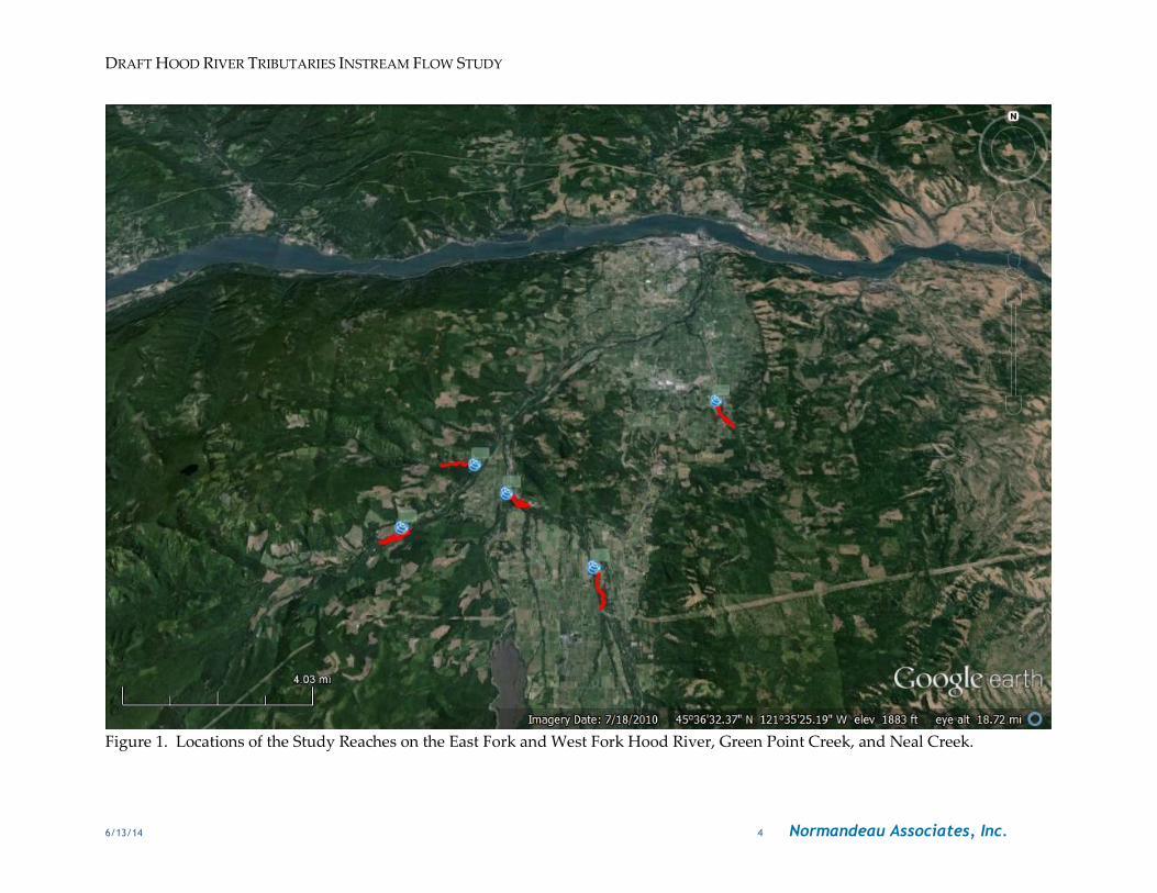
Figure 1. Locations of the Study Reaches on the East Fork and West Fork Hood River, Green Point Creek, and Neal Creek. .................................................... 4
Figure 2. Generic habitat index curve illustrating equal AWS values at two different flows. ...................................................................................... 14
Figure 3. Time series process. ......................................................................... 15
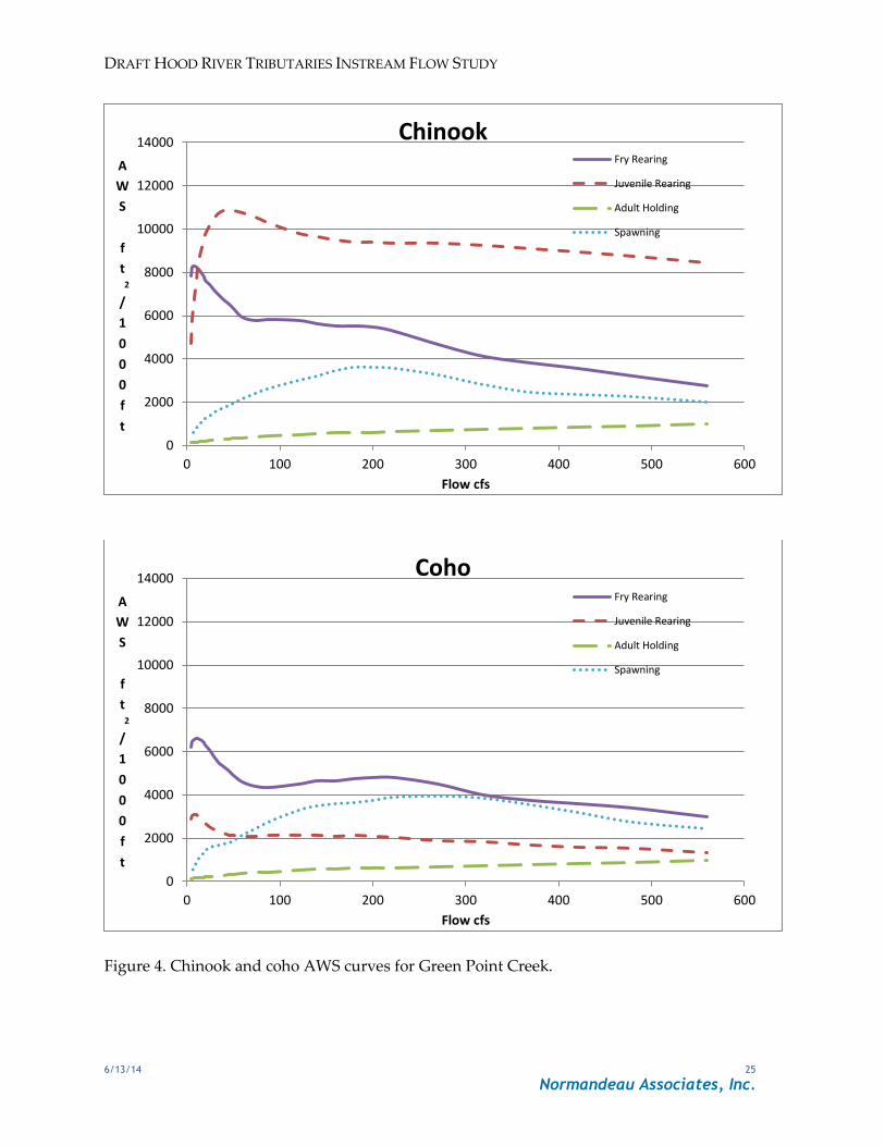
Figure 4. Chinook and coho AWS curves for Green Point Creek. ................................. 25
Figure 5. Steelhead and cutthroat AWS curves for Green Point Creek. ......................... 26
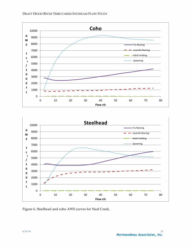
Figure 6. Steelhead and coho AWS curves for Neal Creek. ........................................ 27
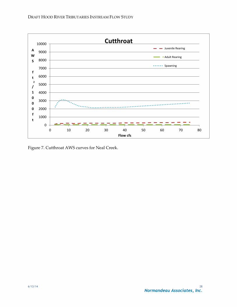
Figure 7. Cutthroat AWS curves for Neal Creek. .................................................... 28
Figure 8. Chinook and coho AWS curves for E.F. Hood (upper). ................................. 29
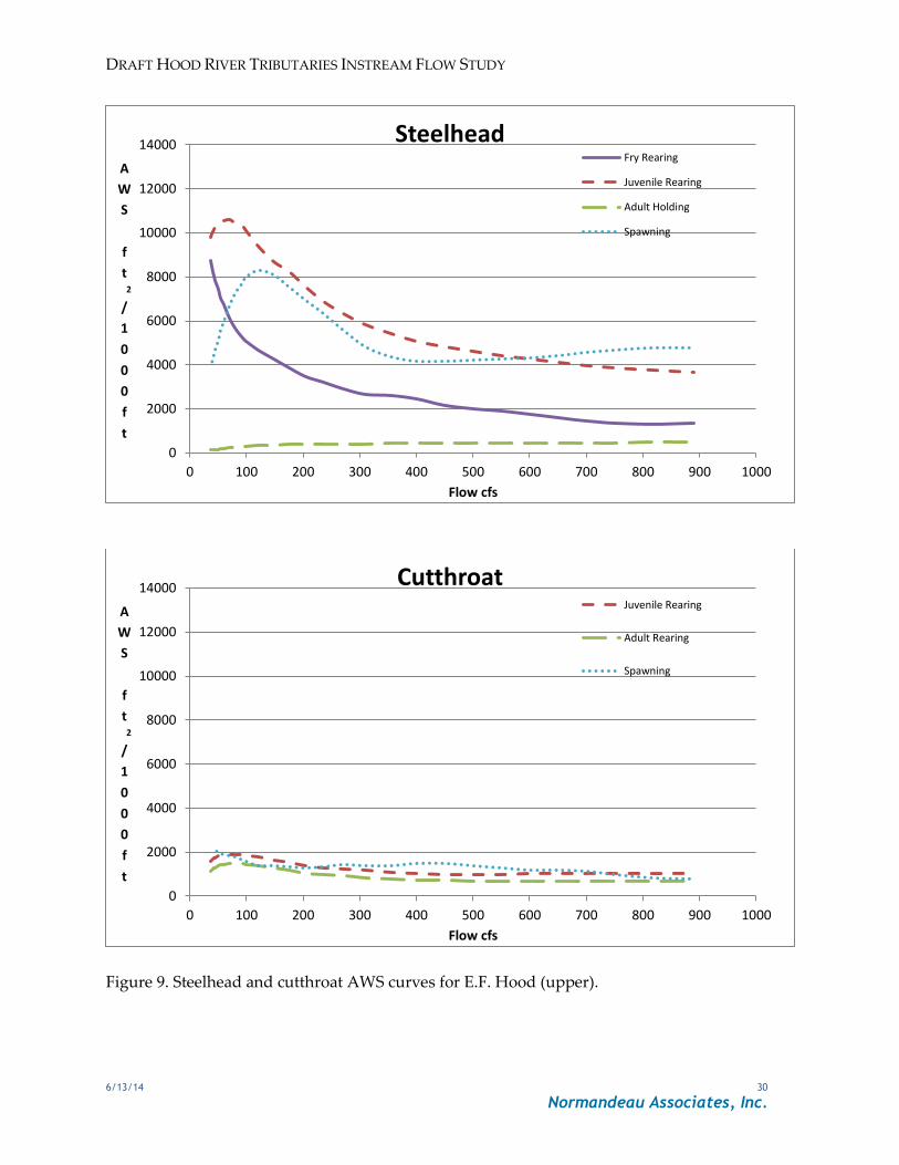
Figure 9. Steelhead and cutthroat AWS curves for E.F. Hood (upper). ......................... 30
Figure 10. Chinook and coho AWS curves for E.F. Hood (lower). ................................ 31
Figure 11. Steelhead and cutthroat AWS curves for E.F. Hood (lower). ........................ 32
Figure 12. Chinook and coho AWS curves for W.F. Hood River. .................................. 33
Figure 13. Steelhead and cutthroat AWS curves for W.F. Hood River. .......................... 34
Figure 14. Bull trout AWS curves for W.F. Hood River. ............................................ 35
Figure 15. Flow time series (top) and Chinook juvenile habitat time series (bottom) for 30 years of historic flow in the East Fork Hood River.. ............................ 39
Figure 16. Overlay of flow time series and Chinook juvenile habitat time series for a selected time period from the upper East Fork Hood River. ..................... 40
Figure 17. Raster hydrograph of historic flows in the Upper East Fork Hood River. .......... 41
Figure 18. Raster plot of Chinook juvenile habitat (AWS) for historic flows in the Upper East Fork Hood River. ................................................................... 42
Figure 19. Chinook juvenile WUA/AWS curve for the upper East Fork Hood River. ........... 43
Figure 20. Flow duration curves for 13 flow scenarios on upper East Fork Hood River. Top, 0-100% exceedance; bottom, 5-95% exceedance. ............................ 44
Figure 21. Chinook juvenile habitat duration for the upper East Fork Hood River. ........... 45
Figure 22. Flow duration curves for Chinook spawning for 13 flow scenarios on the upper East Fork Hood River. Top, 0-100% exceedance; bottom, 5-95% exceedance. .............................................................................. 46
Figure 23. Chinook spawning habitat duration for the upper East Fork Hood River. .......... 47
DRAFT HOOD RIVER TRIBUTARIES INSTREAM FLOW STUDY
6/13/14 v Normandeau Associates, Inc.
Figure 24. Change in AWS between the historic climate scenario and scenario 5.3 for Chinook rearing habitat in the East Fork Hood River. ............................. 50
Figure 25. Upper East Fork Hood historical raster hydrograph with black dots plotted for each day that the AWS is greater or equal than the 50% exceedance value for juvenile Chinook rearing. .......................................................... 51
Figure 26. Upper East Fork Hood climate scenario 5.3 raster hydrograph with black dots plotted for each day that the AWS is greater or equal than the 50% exceedance value for juvenile Chinook rearing. .................................... 52
DRAFT HOOD RIVER TRIBUTARIES INSTREAM FLOW STUDY
6/13/14 vi Normandeau Associates, Inc.
List of Tables
Page
Table 1. Substrate size and codes. ..................................................................... 8
Table 2. Cover types and codes. ........................................................................ 8
Table 3. Target species and life stages selected for modeling in each of the five stream reaches. ................................................................................... 12
Table 4. Habitat mapping summary for Green Point Creek. ...................................... 16
Table 5. Habitat mapping summary for Neal Creek ................................................ 16
Table 6. Habitat mapping summary for East Fork Hood River (lower). ......................... 17
Table 7. Habitat mapping summary for East Fork Hood River (upper). ......................... 17
Table 8. Habitat mapping summary for West Fork Hood River. .................................. 18
Table 9. Number of transects by habitat type and reach with habitat selector identified (*). ......................................................................................... 18
Table 10. Measured flow, calibration flow (velocity acquisition flow), stage-discharge rating curve mean error and method and VAF for transects in five reaches of the Hood River. ....................................................................... 20
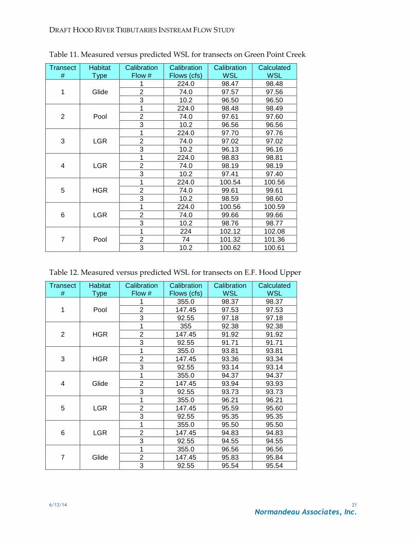
Table 11. Measured versus predicted WSL for transects on Green Point Creek ............... 21
Table 12. Measured versus predicted WSL for transects on E.F. Hood Upper .................. 21
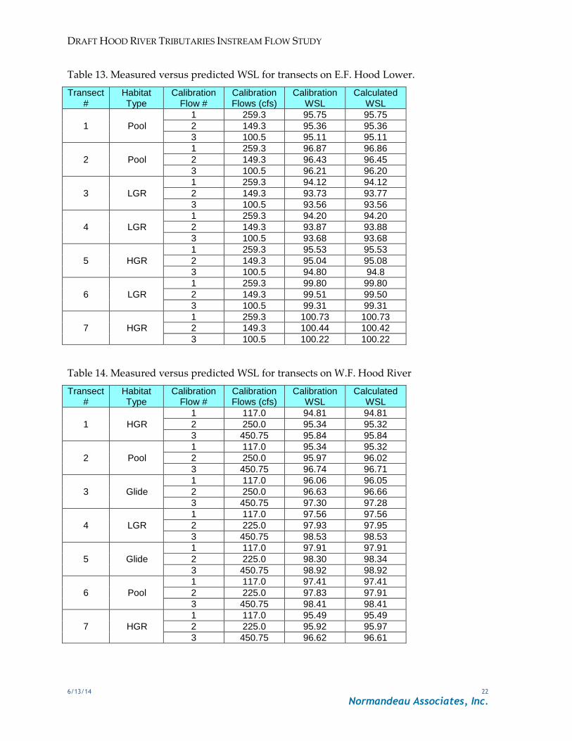
Table 13. Measured versus predicted WSL for transects on E.F. Hood Lower. ................. 22
Table 14. Measured versus predicted WSL for transects on W.F. Hood River .................. 22
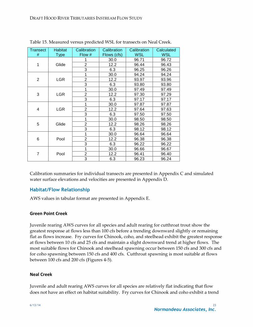
Table 15. Measured versus predicted WSL for transects on Neal Creek. ....................... 23
Table 16. Stream reaches, species and life stages utilized in habitat time series. ........... 36
Table 17. Species and life stage periodicity table for the Hood River Tributaries Instream Flow Study time series. ................................................................. 36
Table 18. Hydrology scenarios used to evaluate potential changes in flow and habitat of selected fish species and life stages in the Hood River tributaries study. ...... 37
DRAFT HOOD RIVER TRIBUTARIES INSTREAM FLOW STUDY
6/13/14 1
Normandeau Associates, Inc.
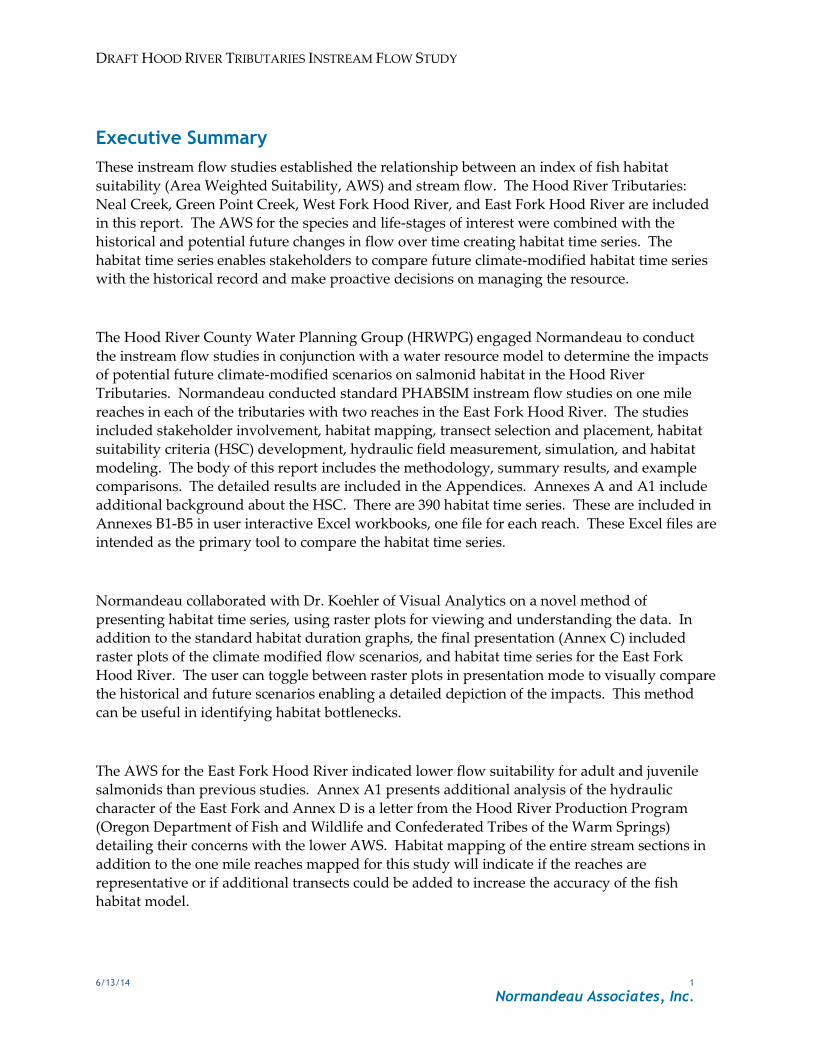
Executive Summary
These instream flow studies established the relationship between an index of fish habitat
suitability (Area Weighted Suitability, AWS) and stream flow. The Hood River Tributaries:
Neal Creek, Green Point Creek, West Fork Hood River, and East Fork Hood River are included in this report. The AWS for the species and life-stages of interest were combined with the
historical and potential future changes in flow over time creating habitat time series. The
habitat time series enables stakeholders to compare future climate-modified habitat time series with the historical record and make proactive decisions on managing the resource.
The Hood River County Water Planning Group (HRWPG) engaged Normandeau to conduct
the instream flow studies in conjunction with a water resource model to determine the impacts of potential future climate-modified scenarios on salmonid habitat in the Hood River
Tributaries. Normandeau conducted standard PHABSIM instream flow studies on one mile
reaches in each of the tributaries with two reaches in the East Fork Hood River. The studies included stakeholder involvement, habitat mapping, transect selection and placement, habitat
suitability criteria (HSC) development, hydraulic field measurement, simulation, and habitat
modeling. The body of this report includes the methodology, summary results, and example comparisons. The detailed results are included in the Appendices. Annexes A and A1 include
additional background about the HSC. There are 390 habitat time series. These are included in
Annexes B1-B5 in user interactive Excel workbooks, one file for each reach. These Excel files are intended as the primary tool to compare the habitat time series.
Normandeau collaborated with Dr. Koehler of Visual Analytics on a novel method of
presenting habitat time series, using raster plots for viewing and understanding the data. In addition to the standard habitat duration graphs, the final presentation (Annex C) included
raster plots of the climate modified flow scenarios, and habitat time series for the East Fork
Hood River. The user can toggle between raster plots in presentation mode to visually compare the historical and future scenarios enabling a detailed depiction of the impacts. This method
can be useful in identifying habitat bottlenecks.
The AWS for the East Fork Hood River indicated lower flow suitability for adult and juvenile salmonids than previous studies. Annex A1 presents additional analysis of the hydraulic
character of the East Fork and Annex D is a letter from the Hood River Production Program
(Oregon Department of Fish and Wildlife and Confederated Tribes of the Warm Springs) detailing their concerns with the lower AWS. Habitat mapping of the entire stream sections in
addition to the one mile reaches mapped for this study will indicate if the reaches are
representative or if additional transects could be added to increase the accuracy of the fish habitat model.
DRAFT HOOD RIVER TRIBUTARIES INSTREAM FLOW STUDY
6/13/14 2
Normandeau Associates, Inc.
Acronyms and Abbreviations
ADCP Acoustic Doppler Current Profiler
AWS Area Weighted Suitability (current name for WUA)
BOR Bureau of Reclamation
CTWS Confederated Tribes of the Warm Springs
HRCWPG Hood River County Water planning Group
HSC Habitat Suitability Criteria
IFG Instream Flow Group
MFID Middle Fork Irrigation District
ODFW Oregon Department of Fish and Wildlife
PHABSIM Physical Habitat Simulation model developed by the U.S. Fish and Wildlife Service
RHABSIM Riverine Habitat Simulation software conversion and enhancement of PHABSIM by TRPA, currently Normandeau Associates
SEFA System for Environmental Flow Analysis, software enhancing the capabilities of RHABSIM, RYHABSIM, and PHABSIM developed by T. Payne, I. Jowett, and B. Milhouse.
TRPA Thomas R. Payne and Associates
WDFW Washington Department of Fish and Wildlife
WSEL Water Surface Elevation
WUA Weighted Usable Area, a Habitat Index (old name for AWS)
Introduction
The Hood River County Water planning Group (HRCWPG) is developing a water resource
model as a tool to assist in the long-term management of water in the Hood River Basin.
Components of the water resource model account for inflows, outflows, and changes in hydrology due to climate change. In order to provide model assessment of fish habitat,
Normandeau was contracted to develop an index relationship of hydraulic fish habitat to flow
in various tributaries to the Hood River.
Normandeau conducted an instream flow study in each of the Hood River Tributaries: East
Fork Hood River, West Fork Hood River, Neal Creek, and Green Point Creek. The objective of the instream flow study was to determine the incremental relationship between stream flow
and an index to physical habitat availability, commonly called weighted usable area (WUA) and
more recently called area weighted suitability (AWS, Jowett et.al. 2014), for the species and life stages of interest.

DRAFT HOOD RIVER TRIBUTARIES INSTREAM FLOW STUDY
6/13/14 3
Normandeau Associates, Inc.
The standard approach to instream flow analysis since 1980 has been the Instream Flow
Incremental Methodology (IFIM). The IFIM is a structured habitat evaluation process initially developed by the Instream Flow Group of the U.S. Fish and Wildlife Service (USFWS) in the late
1970’s to allow evaluation of alternative flow regimes for water development projects (Bovee
and Milhous 1978; Bovee et al. 1998). Techniques used in the IFIM process have continued to evolve since its introduction (Bovee and Zuboy 1988; Bremm 1988; Payne 1987, 1988a, 1988b,
1992). Improvements have been made in the in the approaches to defining study reaches
(Morhardt et al. 1983), in transect selection (Payne 1992), and in the techniques of PHABSIM data collection, computer modeling, and analysis (Milhous et al. 1984). The IFIM may involve
multiple scientific disciplines and stakeholders, in the context of which physical habitat
simulation (PHABSIM) studies are usually designed and implemented. Normandeau utilized PHABSIM for the instream flow model in each of the reaches.
Study Area
The study area was in Hood River County, Washington and included approximately one mile
long reaches in the West Fork Hood River, Green Point Creek, and Neal Creek and two
approximately one mile long reaches in the East Fork Hood River (Figure 1).
DRAFT HOOD RIVER TRIBUTARIES INSTREAM FLOW STUDY
6/13/14 4 Normandeau Associates, Inc.
Figure 1. Locations of the Study Reaches on the East Fork and West Fork Hood River, Green Point Creek, and Neal Creek.
DRAFT HOOD RIVER TRIBUTARIES INSTREAM FLOW STUDY
6/13/14 5
Normandeau Associates, Inc.
Methodology
Development of a relationship between suitable aquatic habitat and river flow for selected
species and life stages within the IFIM/PHABSIM framework depends on the measurement or estimation of physical habitat parameters (depth, velocity, substrate/cover) within the study
reach. Generally, the distribution of these parameters at given river flows are determined at
points along transect lines across the stream channel, positioned to account for spatial and flow-related variability. A variety of hydraulic modeling techniques can be used to simulate water
depth and velocity as a function of river flow; substrate and cover values are generally fixed at a
given point. With physical habitat thus characterized for a range of river flows, the suitability of the habitat (for a particular species and life stage) at each point is scaled from zero to one,
usually by multiplying together the corresponding suitability values for depth, velocity, and
substrate from the appropriate habitat suitability criteria (HSC) curves. These point estimates of suitability are then used to weight the physical area of the study represented by each point, and
the weighted areas are accumulated for the entire study reach to produce an index of useable
habitat as a function of river flow for each species and life stage.
The physical area represented by each transect point depends on the design of the PHABSIM
study. This study used the mesohabitat typing, or habitat mapping, approach originally described by Morhardt et al. (1983) and summarized by Bovee et al. (1998). In this design,
mesohabitats (broadly defined habitat generalizations) were mapped over the entire study
reach, such that each area of the waterway was characterized by a general habitat type, and the total length and proportion of the study reach assigned to each mesohabitat type was
determined.
Physical habitat parameters (river flow dependent depth and velocity, substrate, and cover)
representative of each mesohabitat type were measured or modeled at one or more transects
placed within the mesohabitat area. The exact number and placement of transects placed in a mesohabitat type depended on the proportion of the study reach represented by each
mesohabitat type, as well as practical issues such as accessibility. Generally, the total number of
transects was distributed among mesohabitat types in proportion to the length of the study reach represented by each mesohabitat. The physical area represented by each transect point
was then determined by both the lateral distribution of points on a transect, and the length or
proportion of the study reach that each transect represented.
Stakeholder Involvement
Stakeholders, through the HRCWPG, provided input into the selection of study reaches,
transect locations, species and life-stages of interest, HSC, and calibration flows, as well as reviewing the AWS curves.
DRAFT HOOD RIVER TRIBUTARIES INSTREAM FLOW STUDY
6/13/14 6
Normandeau Associates, Inc.
Habitat Mapping
Habitat mapping consists of identifying the type (e.g. pools, runs, and riffles) and measuring
the length of individual macrohabitat units over the total distance of stream courses within a project area (Morhardt et al. 1983). The method allows each transect where hydraulic data is
collected to be given a weight proportional to the quantity of habitat represented by that
transect. Mapping was conducted by walking the stream channel while deploying biodegradable cotton thread from a surveyor’s hip chain to measure total distance. The location
and length of each individual macrohabitat type was calculated by noting the distance from a
downstream base reference point to upstream boundaries. Reference points were marked using surveyor’s flagging every 500 feet (generally at the nearest hydraulic control) as well as GPS
waypoints. These marks serve as temporary and fixed, known reference points from which to
relocate specific habitat units or other features of interest during the stream studies. Other information noted during the mapping process included estimating the maximum depth for
each pool habitat, and determining whether a unit could be hydraulically modeled.
Normandeau conducted habitat mapping in the five, one-mile reaches using the ODFW Aquatic
Inventories Project Methods for Stream Habitat Surveys (ODFW 2010) as a guide. The basic
survey included identifying habitat types, habitat unit lengths and widths, maximum depth and general substrate and riparian characteristics. Generally, for a PHABSIM study, only habitat
type unit lengths and depths (pools) are used as a basis for selecting transects and weighting of
the habitat model.
The mapping information was used to determine the percentages of various macrohabitats,
assist with selection of study sites, and placement of transects for the hydraulic data collection. Each habitat unit was also evaluated for appropriateness for PHABSIM modeling. Such
conditions that prohibit satisfactory hydraulic simulation included complex hydraulic
conditions associated with strongly transverse flow conditions, plunge pools, or unique split channel configurations. Potentially dangerous and unsafe habitat units, such as those near
dangerous falls or cascades, were also identified for subsequent elimination as candidates for
hydraulic modeling.
The individual macrohabitat identifications and distances were entered into a database
program to create a sequential map of habitat units along the entire length of stream that was
surveyed. The database allowed for the computation of the percent abundance of any
macrohabitat type within the entire study area or within designated reaches. The mapping data
and location markers aided in the relocation of individual habitat units for subsequent
inspection and transect selection.
PHABSIM: Transect Selection and Installation
Habitat mapping forms the basis for transect selection. Percent contribution of individual
habitat types to total habitat is derived from the total length of a given reach. The PHABSIM habitat analysis relies upon hydraulic conditions measured along stream cross sections, or
transects, placed in a variety of different macrohabitats. Habitat unit selection and transect
placement was conducted by Normandeau study leads in conjunction with the HRCWPG and
DRAFT HOOD RIVER TRIBUTARIES INSTREAM FLOW STUDY
6/13/14 7
Normandeau Associates, Inc.
ODFW. Actual habitat unit selection and transect placement was accomplished with a
combination of random selection and professional judgment through the following procedure:
1. The macrohabitat type with the lowest percentage of abundance within each study
segment was used as the basis for random selection (provided that the habitat type was
ecologically significant and made up greater than 5% of the total study reach) and sequentially numbered. Several units were be selected by random number.
2. In the field, the first selected unit was relocated and, if it was modelable, reasonably typical, and it appeared safe to collect hydraulic data during high flows, a transect was placed
that would best represent the habitat type. The second or higher randomly selected units were
used only if initial units were rejected.
3. At least one example of each remaining more-abundant habitat type was then located in
the immediate vicinity of the random transect (upstream or downstream) until the additional study transects were placed in other macrohabitat units. This created a study site and transect
“cluster”, which reduced data collection travel time.
Calibration Flows
Calibration flows are the flows at which water surface elevations and velocities are measured
and from which the model simulations are built. A total of three sets of calibration flow measurements, high, middle and low were made at each transect. Generally the simulations
will be valid for a range of flows from forty percent of the low calibration flow to 250 percent of
the high calibration flow. Velocities at each transect station were measured at the highest safe calibration flow. In the case of unregulated rivers, such as the streams in this study, calibration
flow targets were identified, but the measurements were opportunistic depending on the
weather during the sampling period.
Field Data Collection
Water Surface Elevation and Velocity Measurements
One complete set of depths and velocity measurements was collected at each transect at the
middle flow or the flow level that could be effectively and safely measured. Data was collected using wading/velocity measurement techniques at shallow habitats, and an acoustic Doppler
current profiler (ADCP) mounted on a rigid trimaran in deep pool habitats. The TRDI Rio
Grande 1200kHz ADCP sends and receives acoustic pulses in order to measure the Doppler shift and phase change of the echoes to calculate depth and velocity patterns. Additional
measurements of water surface elevation for each transect and a single discharge measurement
(per transect cluster) were made at the middle and low flow levels.
The amount and type of data collected is suitable for use in a hydraulic simulation with the
PHABSIM computer model in the one-velocity mode for the entire range of flows (Payne 1987). The one-flow model of PHABSIM has been shown to calculate habitat values very close to those
obtained with three full sets of depth and velocity data (Payne 1988b).
DRAFT HOOD RIVER TRIBUTARIES INSTREAM FLOW STUDY
6/13/14 8
Normandeau Associates, Inc.
Field data collection and the form of data recording basically followed the guidelines
established in the IFG field techniques manuals (Trihey and Wegner 1981; Milhous et al. 1984; Bovee 1997). Additional quality control checks that have been found valuable during previous
applications of the simulation models were employed. The techniques for measuring discharge
generally followed the guidelines outlined by Rantz (1982). A minimum of 20 wetted stations per stream transect were be established, with a goal of no less than 15 wetted stations at the
lowest measured flow. The boundaries of each station along each transect were normally at
consistent increments, but significant changes in velocity, substrate, depth, or other important stream habitat features sometimes required additional stationing.
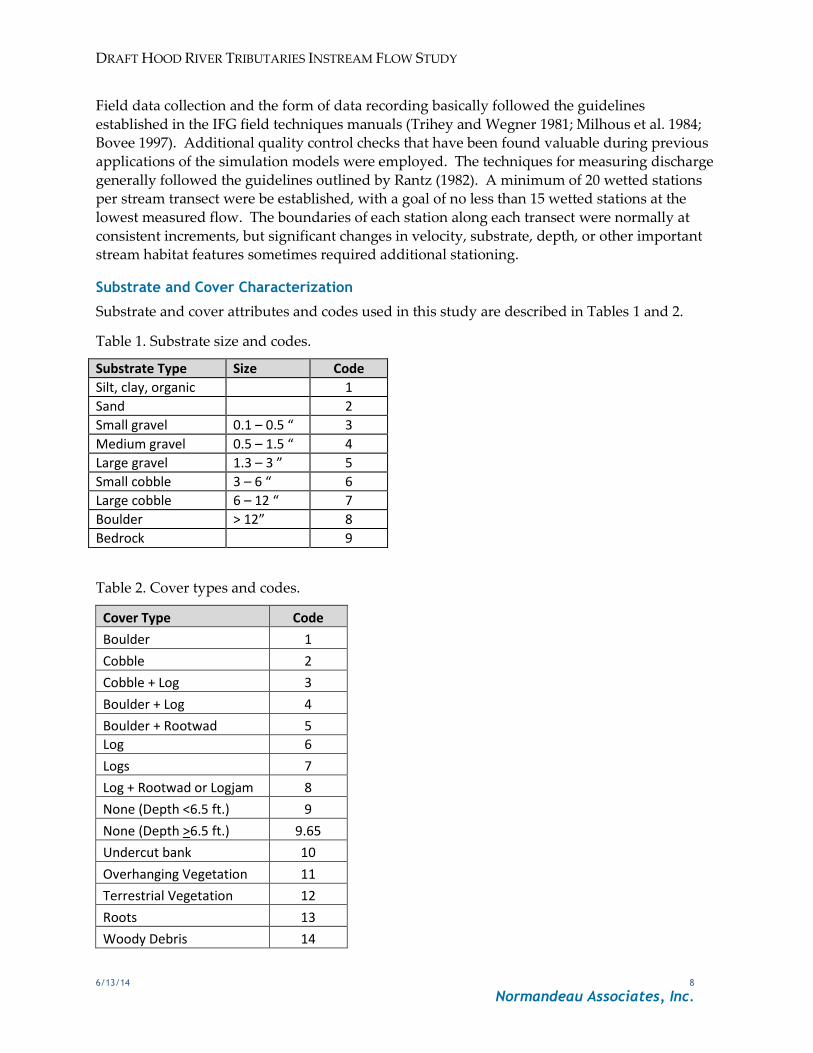
Substrate and Cover Characterization
Substrate and cover attributes and codes used in this study are described in Tables 1 and 2.
Table 1. Substrate size and codes.
Substrate Type Size Code
Silt, clay, organic 1
Sand 2
Small gravel 0.1 – 0.5 “ 3
Medium gravel 0.5 – 1.5 “ 4
Large gravel 1.3 – 3 ” 5
Small cobble 3 – 6 “ 6
Large cobble 6 – 12 “ 7
Boulder > 12” 8
Bedrock 9
Table 2. Cover types and codes.
Cover Type Code
Boulder 1
Cobble 2
Cobble + Log 3
Boulder + Log 4
Boulder + Rootwad 5
Log 6
Logs 7
Log + Rootwad or Logjam 8
None (Depth <6.5 ft.) 9
None (Depth >6.5 ft.) 9.65
Undercut bank 10
Overhanging Vegetation 11
Terrestrial Vegetation 12
Roots 13
Woody Debris 14
DRAFT HOOD RIVER TRIBUTARIES INSTREAM FLOW STUDY
6/13/14 9
Normandeau Associates, Inc.
Quality Assurance/Quality Control
To assure quality control in the collection of field data, the following data collection procedures and protocols were utilized:
Staff gauges were established and continually monitored throughout the course of collecting data. If significant changes occurred, water surface elevations were re-measured following
collection of transect water velocity data.
Independent benchmarks were established for each set of transects. The benchmark was an
immovable tree, boulder, or other naturally occurring object not subject to tampering. Upon
establishment of headpin and tailpin elevations, a level loop was shot to check the auto-level instrument for accuracy. Acceptable error tolerances on level loop measurements were set at
0.02 feet. This tolerance was also applicable to both headpin and tailpin measurements, unless
extenuating circumstances (e.g., pins under sloped banks, shots through dense foliage) accounted for the discrepancies, and the accompanying headpin or tailpin met the tolerance
criteria.
Water surface elevations were measured on both banks on each transect. If possible, on more
complex and uneven transects, such as riffles, water surface elevations were also measured at
multiple locations across a transect. An attempt was made to measure water surface elevations at the same location (station or distance from pin) across each transect at each calibration flow.
Water surface elevation measurements were obtained by placing the bottom of the stadia rod at
the water surface until a meniscus formed at the base or selecting a stable area next to the water’s edge.
Pin and water surface elevations were calculated on-site during field measurement and compared to previous measurements. Changes in stage since the previous flow measurement
were calculated. Patterns of stage change were compared between transects and determined if
reasonable. If any discrepancies were discovered, potential sources of error were explored, corrected where possible, and noted.
The ADCP was used to collect water velocity data from stations along each transect where wading was not possible. High-quality and well-maintained current velocity meters were used
to collect velocities of shallower, edge cell velocity data.
Prior to deployment, the ADCP was system checked, compass calibrated, moving bed test
performed, and user configured for each individual transect with appropriate commands for
the existing environmental conditions. Often several transect measurements were necessary to obtain the optimum configuration. Each transect measurement length and discharge
calculation was compared to the actual values or to repetitive measurements in order to ensure
accurate bottom tracking and velocity measurements. Real time graphic depictions of depth and velocity were examined during data collection for inconsistencies and obvious errors. As a
precaution against data loss, all electronic data files were copied onto a separate USB drive at
the end of each field day.
DRAFT HOOD RIVER TRIBUTARIES INSTREAM FLOW STUDY
6/13/14 10
Normandeau Associates, Inc.
All calculations were completed in the field, given adequate time and daylight. Pin elevations
and changes in water surface elevations were compared between flows on the same transect. Discharges were calculated on-site and were compared between transects during the same flow
(high, mid, and low). If an excessive amount of discharge (greater than 10% of the stream flow)
was noted for an individual transect cell, additional adjacent stations were established to more precisely define the velocity distribution patterns at that portion of the transect.
Photographs were taken of all transects, downstream, across, and upstream at the three calibration flows. Photographs were taken from the same location at each of the flows, if
possible. Photographs provided a valuable record of physical conditions and water surface
levels that were utilized during hydraulic model calibration.
All data (stationing, depth profiles, velocities, substrate/cover codes) were entered into the
RHABSIM computer files. Internal data graphing routines were then used to review the bottom and velocity profiles for each transect separately and in context with others for quality control
purposes. All data gaps (e.g., missing velocities) or discrepancies (e.g., conflicting records) were
identified and corrected using available sources, such as field notes, photographs, or adjacent data points.
Transect Weighting
The number of transects selected for each habitat type was determined by the percentage of the
study reach represented by each habitat type. In this way each habitat type was represented approximately in proportion to that which was mapped. Each transect was then weighted so
that each habitat type was represented in the exact proportion to that existent in the study area.
Hydraulic Simulation
The purpose of hydraulic simulation under the PHABSIM framework is to simulate depths and
velocities in streams under varying stream flow conditions. Simulated depth and velocity data were then used to calculate the physical habitat, either with or without substrate and/or cover
information. All data was entered into the RHABSIM software used for this analysis.
Water Surface Prediction
The water surface elevations, in conjunction with the transect profiles, were used to determine
water depths at each flow. Water depth is an important parameter for determining the physical
habitat suitability. Either an empirical log/log regression formula of stage and flow based on measured data or a channel conveyance method (MANSQ) that relies on the Manning’s N
roughness equation was used to create the rating curves.
The log/log regression method uses a stage-discharge relationship to determine water surface
elevations. Each cross section is treated independently of all others in the data set. A minimum
of three stage-discharge measurement pairs were used to calibrate the stage-discharge relationship. The quality of the rating curves is evaluated by examination of mean error and
slope output from the model. Mean errors of less than 10% is considered acceptable and less
than 5% is very good. In general the slope between groups of transects should be similar.
MANSQ only requires a single stage-discharge pair and utilizes Manning’s equation and
channel shape to determine a rating curve; however, it is generally validated by additional
DRAFT HOOD RIVER TRIBUTARIES INSTREAM FLOW STUDY
6/13/14 11
Normandeau Associates, Inc.
stage-discharge measurements. This modeling method involves an iterative process where a
beta coefficient is adjusted until a satisfactory result is obtained. In situations where irregular channel features occur on a cross section, for instance bars or terraces, MANSQ is often better at
predicting higher stages than log/log. MANSQ is most often used on riffle or run transects and
is generally not considered as effective in establishing a rating curves for transects that have backwater effects from downstream controls, such as pools. It can also be useful as a test and
verification of log/log relationships.
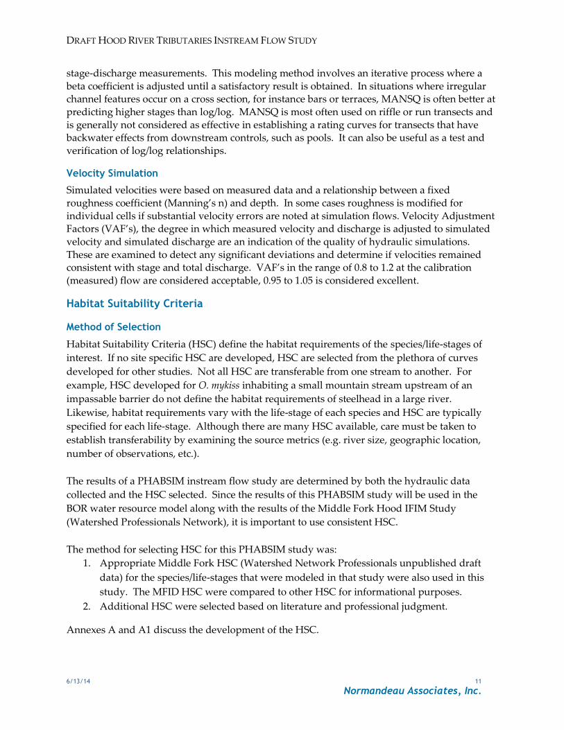
Velocity Simulation
Simulated velocities were based on measured data and a relationship between a fixed
roughness coefficient (Manning’s n) and depth. In some cases roughness is modified for
individual cells if substantial velocity errors are noted at simulation flows. Velocity Adjustment Factors (VAF’s), the degree in which measured velocity and discharge is adjusted to simulated
velocity and simulated discharge are an indication of the quality of hydraulic simulations.
These are examined to detect any significant deviations and determine if velocities remained consistent with stage and total discharge. VAF’s in the range of 0.8 to 1.2 at the calibration
(measured) flow are considered acceptable, 0.95 to 1.05 is considered excellent.
Habitat Suitability Criteria
Method of Selection
Habitat Suitability Criteria (HSC) define the habitat requirements of the species/life-stages of
interest. If no site specific HSC are developed, HSC are selected from the plethora of curves
developed for other studies. Not all HSC are transferable from one stream to another. For
example, HSC developed for O. mykiss inhabiting a small mountain stream upstream of an
impassable barrier do not define the habitat requirements of steelhead in a large river.
Likewise, habitat requirements vary with the life-stage of each species and HSC are typically
specified for each life-stage. Although there are many HSC available, care must be taken to
establish transferability by examining the source metrics (e.g. river size, geographic location,
number of observations, etc.).
The results of a PHABSIM instream flow study are determined by both the hydraulic data
collected and the HSC selected. Since the results of this PHABSIM study will be used in the
BOR water resource model along with the results of the Middle Fork Hood IFIM Study
(Watershed Professionals Network), it is important to use consistent HSC.
The method for selecting HSC for this PHABSIM study was:
1. Appropriate Middle Fork HSC (Watershed Network Professionals unpublished draft
data) for the species/life-stages that were modeled in that study were also used in this
study. The MFID HSC were compared to other HSC for informational purposes.
2. Additional HSC were selected based on literature and professional judgment.
Annexes A and A1 discuss the development of the HSC.
DRAFT HOOD RIVER TRIBUTARIES INSTREAM FLOW STUDY
6/13/14 12
Normandeau Associates, Inc.
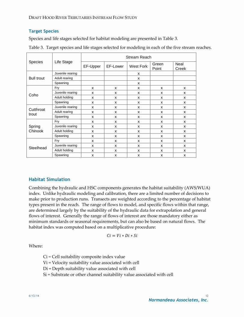
Target Species
Species and life stages selected for habitat modeling are presented in Table 3.
Table 3. Target species and life stages selected for modeling in each of the five stream reaches.
Species Life Stage
Stream Reach
EF-Upper EF-Lower West Fork Green Point
Neal Creek
Bull trout
Juvenile rearing x Adult rearing x Spawning x
Coho
Fry x x x x x Juvenile rearing x x x x x Adult holding x x x x x Spawning x x x x x
Cutthroat trout
Juvenile rearing x x x x x Adult rearing x x x x x Spawning x x x x x
Spring Chinook
Fry x x x x x Juvenile rearing x x x x x Adult holding x x x x x Spawning x x x x x
Steelhead
Fry x x x x x Juvenile rearing x x x x x Adult holding x x x x x Spawning x x x x x
Habitat Simulation
Combining the hydraulic and HSC components generates the habitat suitability (AWS/WUA)
index. Unlike hydraulic modeling and calibration, there are a limited number of decisions to make prior to production runs. Transects are weighted according to the percentage of habitat
types present in the reach. The range of flows to model, and specific flows within that range,
are determined largely by the suitability of the hydraulic data for extrapolation and general flows of interest. Generally the range of flows of interest are those mandatory either as
minimum standards or seasonal requirements, but can also be based on natural flows. The
habitat index was computed based on a multiplicative procedure:
Where:
Ci = Cell suitability composite index value
Vi = Velocity suitability value associated with cell
Di = Depth suitability value associated with cell
Si = Substrate or other channel suitability value associated with cell

DRAFT HOOD RIVER TRIBUTARIES INSTREAM FLOW STUDY
6/13/14 13
Normandeau Associates, Inc.
The cell composite number is then multiplied by the cell width to produce number of square
feet of area in that cell. For each transect, all the cells' areas are summed to produce a total number of square feet of usable habitat available at a specified flow. This result is then
multiplied by the percentage the individual transect represents as a proportion of all transects
being modeled. All transect results are then summed to produce overall habitat suitability in square feet.
Time Series Analysis
Utilization and interpretation of habitat modeling output, namely habitat index curves, presents
a challenge from both a technical and functional perspective. The habitat versus flow
relationships derived from PHABSIM represent a conceptual association between flow and
habitat. Though some basic inference can be made from this relationship, evaluation without
incorporating flow regimes can lead to erroneous interpretations. This analysis is particularly
valuable when considering a suite of species and life stages with varying habitat versus flow
relationships, and instances when known life history needs may not be directly exhibited in the
habitat versus flow relationship output from PHABSIM.
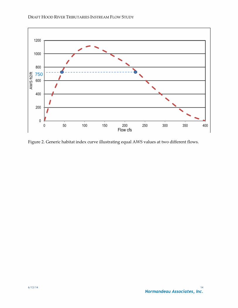
The tendency to look at the maximum or “peak” of a habitat index curve greatly oversimplifies
the results. For example, maximum spawning habitat may occur at a flow that rarely exists in a
given reach. Additionally, the amount of habitat can be the same at two flows, one lower and
one higher than the maximum (Figure 2). Because the amount of habitat available at any given
time of year is a function of hydrology, incorporating a time-series analysis provides a more
realistic view of available habitat. Such an analysis is important when determining effects of
different flow regimes that may result from changes in water usage. Times series involves
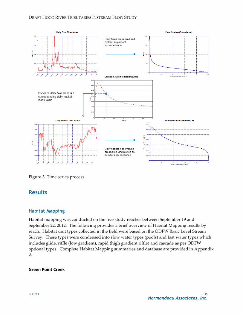
matching the habitat index for a given species or life stage to flow, as illustrated in Figure 3.
The major basis for habitat time series analysis is that habitat is a function of stream flow and
that stream flow varies over time. Habitat time series displays the temporal habitat change for a
particular species and life stage during selected seasons or critical time periods under various
flow scenarios. Typically results are represented by habitat duration curves indicating the
quantity of habitat that is equaled or exceeded over the selected time period.
DRAFT HOOD RIVER TRIBUTARIES INSTREAM FLOW STUDY
6/13/14 14
Normandeau Associates, Inc.
Figure 2. Generic habitat index curve illustrating equal AWS values at two different flows.
0
200
400
600
800
1000
1200
0 50 100 150 200 250 300 350 400
AW
S ft2
/ft
Flow cfs
750
DRAFT HOOD RIVER TRIBUTARIES INSTREAM FLOW STUDY
6/13/14 15
Normandeau Associates, Inc.
Figure 3. Time series process.
Results
Habitat Mapping
Habitat mapping was conducted on the five study reaches between September 19 and
September 22, 2012. The following provides a brief overview of Habitat Mapping results by
reach. Habitat unit types collected in the field were based on the ODFW Basic Level Stream
Survey. These types were condensed into slow water types (pools) and fast water types which
includes glide, riffle (low gradient), rapid (high gradient riffle) and cascade as per ODFW
optional types. Complete Habitat Mapping summaries and database are provided in Appendix
A.
Green Point Creek
DRAFT HOOD RIVER TRIBUTARIES INSTREAM FLOW STUDY
6/13/14 16
Normandeau Associates, Inc.
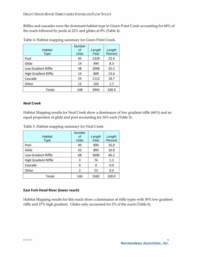
Riffles and cascades were the dominant habitat type in Green Point Creek accounting for 68% of
the reach followed by pools at 22% and glides at 8% (Table 4).
Table 4. Habitat mapping summary for Green Point Creek.
Habitat Type
Number of
Units Length Feet
Length Percent
Pool 45 1329 22.4
Glide 14 494 8.3
Low Gradient Riffle 38 2098 35.3
High Gradient Riffle 14 809 13.6
Cascade 25 1112 18.7
Other 12 103 1.7
Totals 148 5945 100.0
Neal Creek
Habitat Mapping results for Neal Creek show a dominance of low gradient riffle (66%) and an
equal proportion of glide and pool accounting for 16% each (Table 5).
Table 5. Habitat mapping summary for Neal Creek
Habitat Type
Number of
Units Length Feet
Length Percent
Pool 40 894 16.0
Glide 33 895 16.0
Low Gradient Riffle 68 3696 66.2
High Gradient Riffle 3 74 1.3
Cascade 0 0 0.0
Other 2 23 0.4
Totals 146 5582 100.0
East Fork Hood River (lower reach)
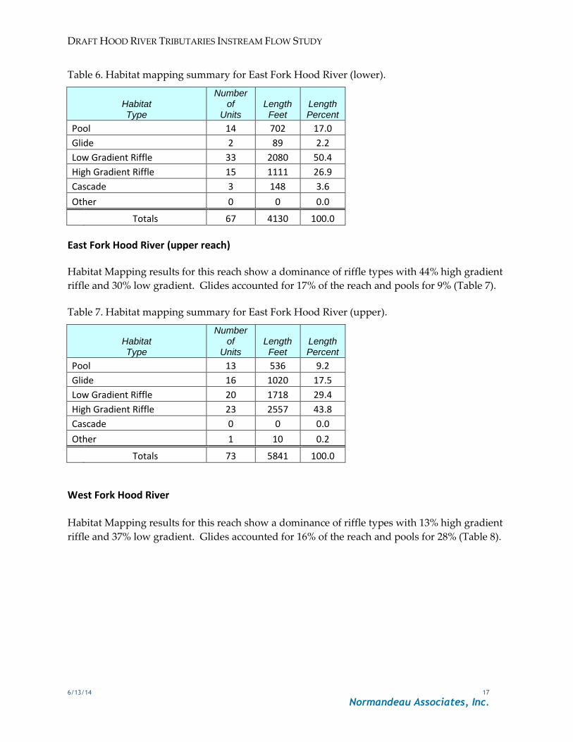
Habitat Mapping results for this reach show a dominance of riffle types with 50% low gradient
riffle and 27% high gradient. Glides only accounted for 2% of the reach (Table 6).
DRAFT HOOD RIVER TRIBUTARIES INSTREAM FLOW STUDY
6/13/14 17
Normandeau Associates, Inc.
Table 6. Habitat mapping summary for East Fork Hood River (lower).
Habitat Type
Number of
Units Length Feet
Length Percent
Pool 14 702 17.0
Glide 2 89 2.2
Low Gradient Riffle 33 2080 50.4
High Gradient Riffle 15 1111 26.9
Cascade 3 148 3.6
Other 0 0 0.0
Totals 67 4130 100.0
East Fork Hood River (upper reach)
Habitat Mapping results for this reach show a dominance of riffle types with 44% high gradient
riffle and 30% low gradient. Glides accounted for 17% of the reach and pools for 9% (Table 7).
Table 7. Habitat mapping summary for East Fork Hood River (upper).
Habitat Type
Number of
Units Length Feet
Length Percent
Pool 13 536 9.2
Glide 16 1020 17.5
Low Gradient Riffle 20 1718 29.4
High Gradient Riffle 23 2557 43.8
Cascade 0 0 0.0
Other 1 10 0.2
Totals 73 5841 100.0
West Fork Hood River Habitat Mapping results for this reach show a dominance of riffle types with 13% high gradient
riffle and 37% low gradient. Glides accounted for 16% of the reach and pools for 28% (Table 8).

DRAFT HOOD RIVER TRIBUTARIES INSTREAM FLOW STUDY
6/13/14 18
Normandeau Associates, Inc.
Table 8. Habitat mapping summary for West Fork Hood River.
Habitat Type
Number of
Units Length Feet
Length Percent
Pool 13 1452 27.8
Glide 16 821 15.7
Low Gradient Riffle 19 1953 37.4
High Gradient Riffle 9 671 12.8
Cascade 4 327 6.3
Other 0 0 0.0
Totals 61 5224 100.0
Study Site and Transect Selection
Study sites were established by randomly selecting the least available habitat type, locating the
habitat unit and placing a transect to represent the unit. Additional transects were then
established in other habitat types in the immediate vicinity in general proportion to availability.
A total of 7 cross sections were used to represent hydraulic and habitat conditions in each reach
(Table 9).
Table 9. Number of transects by habitat type and reach with habitat selector identified (*).
Number of Transects by Reach and Habitat Type
Habitat Type
Green Point Creek Neal Creek
E.F. Hood River (upper)
E.F. Hood River (lower)
West Fork Hood River
Pool 2 2 1* 2* 2
Glide 1* 2* 2 0 2
Low Gradient Riffle 3 3 2 3 2
High Gradient Riffle 1 0 2 2 1*
Cascade 0 0 0 0 0
Total 7 7 7 7 7
Hydraulic Simulation
Field data collection took place between September and December 2012. Low flow was
measured in late September in all reaches except Neal Creek, which was deemed to be the approximate middle flow target. Middle flow and velocity acquisition took place in all other
reaches in late October and high flow occurred in late November and early December. Transect
profiles, calibration velocities, and calibration flow water surface elevation plots are depicted in Appendix B.
DRAFT HOOD RIVER TRIBUTARIES INSTREAM FLOW STUDY
6/13/14 19
Normandeau Associates, Inc.
Stage-Discharge
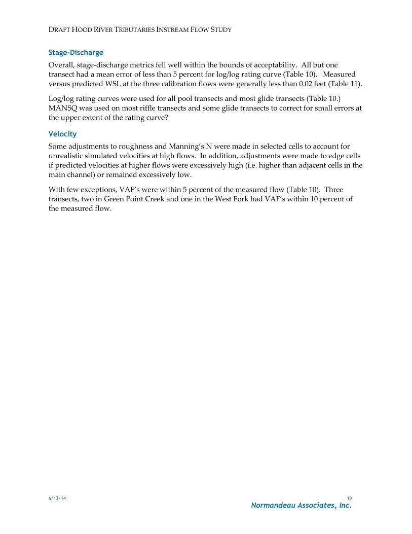
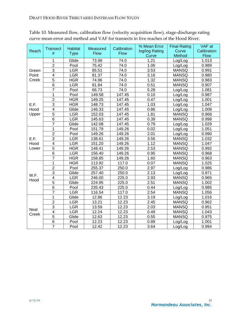
Overall, stage-discharge metrics fell well within the bounds of acceptability. All but one transect had a mean error of less than 5 percent for log/log rating curve (Table 10). Measured
versus predicted WSL at the three calibration flows were generally less than 0.02 feet (Table 11).
Log/log rating curves were used for all pool transects and most glide transects (Table 10.)
MANSQ was used on most riffle transects and some glide transects to correct for small errors at
the upper extent of the rating curve?
Velocity
Some adjustments to roughness and Manning’s N were made in selected cells to account for
unrealistic simulated velocities at high flows. In addition, adjustments were made to edge cells
if predicted velocities at higher flows were excessively high (i.e. higher than adjacent cells in the main channel) or remained excessively low.
With few exceptions, VAF’s were within 5 percent of the measured flow (Table 10). Three transects, two in Green Point Creek and one in the West Fork had VAF’s within 10 percent of
the measured flow.
DRAFT HOOD RIVER TRIBUTARIES INSTREAM FLOW STUDY
6/13/14 20
Normandeau Associates, Inc.
Table 10. Measured flow, calibration flow (velocity acquisition flow), stage-discharge rating
curve mean error and method and VAF for transects in five reaches of the Hood River.
Reach Transect
# Habitat Type
Measured Flow
Calibration Flow
% Mean Error log/log Rating
Curve
Final Rating Curve
Method
VAF at Calibration
Flow
Green Point Creek
1 Glide 73.98 74.0 1.21 Log/Log 1.013
2 Pool 75.42 74.0 1.06 Log/Log 0.989
3 LGR 85.51 74.0 3.53 MANSQ 0.991
4 LGR 81.37 74.0 3.16 MANSQ 0.980
5 HGR 74.96 74.0 1.32 MANSQ 0.983
6 LGR 81.84 74.0 0.51 MANSQ 0.907
7 Pool 66.73 74.0 5.28 Log/Log 1.081
E.F. Hood Upper
1 Pool 149.58 147.45 0.10 Log/Log 0.987
2 HGR 149.25 147.45 0.47 Log/Log 1.001
3 HGR 148.73 147.45 1.03 Log/Log 1.047
4 Glide 146.33 147.45 0.86 Log/Log 1.008
5 LGR 152.03 147.45 1.81 MANSQ 0.968
6 LGR 145.63 147.45 0.39 MANSQ 0.998
7 Glide 142.08 147.45 0.79 Log/Log 1.029
E.F. Hood Lower
1 Pool 151.79 149.26 0.02 Log/Log 1.051
2 Pool 149.26 149.26 2.01 Log/Log 0.990
3 LGR 138.61 149.26 3.56 MANSQ 1.032
4 LGR 151.20 149.26 1.12 MANSQ 1.047
5 HGR 148.41 149.26 2.53 MANSQ 0.992
6 LGR 156.40 149.26 0.95 MANSQ 0.968
7 HGR 158.85 149.26 1.60 MANSQ 0.963
W.F. Hood
1 HGR 113.92 117.0 0.07 MANSQ 1.025
2 Pool 255.37 250.0 2.97 Log/Log 0.986
3 Glide 257.40 250.0 2.13 Log/Log 0.971
4 LGR 246.00 225.0 2.93 MANSQ 0.965
5 Glide 224.95 225.0 2.51 MANSQ 1.002
6 Pool 235.43 225.0 0.44 Log/Log 0.985
7 LGR 116.54 117.0 2.54 MANSQ 1.056
Neal Creek
1 Glide 12.86 12.23 3.19 Log/Log 1.016
2 LGR 13.21 12.23 2.45 MANSQ 0.962
3 LGR 13.59 12.23 2.03 MANSQ 0.951
4 LGR 12.24 12.23 0.49 MANSQ 1.043
5 Glide 12.63 12.23 0.55 MANSQ 0.975
6 Pool 12.23 12.23 0.89 Log/Log 1.001
7 Pool 12.42 12.23 3.64 Log/Log 0.994
DRAFT HOOD RIVER TRIBUTARIES INSTREAM FLOW STUDY
6/13/14 21
Normandeau Associates, Inc.
Table 11. Measured versus predicted WSL for transects on Green Point Creek
Transect #
Habitat Type
Calibration Flow #
Calibration Flows (cfs)
Calibration WSL
Calculated WSL
1 224.0 98.47 98.48
1 Glide 2 74.0 97.57 97.56
3 10.2 96.50 96.50
1 224.0 98.48 98.49
2 Pool 2 74.0 97.61 97.60
3 10.2 96.56 96.56
1 224.0 97.70 97.76
3 LGR 2 74.0 97.02 97.02
3 10.2 96.13 96.16
1 224.0 98.83 98.81
4 LGR 2 74.0 98.19 98.19
3 10.2 97.41 97.40
1 224.0 100.54 100.56
5 HGR 2 74.0 99.61 99.61
3 10.2 98.59 98.60
1 224.0 100.56 100.59
6 LGR 2 74.0 99.66 99.66
3 10.2 98.76 98.77
1 224 102.12 102.08
7 Pool 2 74 101.32 101.36
3 10.2 100.62 100.61
Table 12. Measured versus predicted WSL for transects on E.F. Hood Upper
Transect #
Habitat Type
Calibration Flow #
Calibration Flows (cfs)
Calibration WSL
Calculated WSL
1 355.0 98.37 98.37
1 Pool 2 147.45 97.53 97.53
3 92.55 97.18 97.18
1 355 92.38 92.38
2 HGR 2 147.45 91.92 91.92
3 92.55 91.71 91.71
1 355.0 93.81 93.81
3 HGR 2 147.45 93.36 93.34
3 92.55 93.14 93.14
1 355.0 94.37 94.37
4 Glide 2 147.45 93.94 93.93
3 92.55 93.73 93.73
1 355.0 96.21 96.21
5 LGR 2 147.45 95.59 95.60
3 92.55 95.35 95.35
1 355.0 95.50 95.50
6 LGR 2 147.45 94.83 94.83
3 92.55 94.55 94.55
1 355.0 96.56 96.56
7 Glide 2 147.45 95.83 95.84
3 92.55 95.54 95.54
DRAFT HOOD RIVER TRIBUTARIES INSTREAM FLOW STUDY
6/13/14 22
Normandeau Associates, Inc.
Table 13. Measured versus predicted WSL for transects on E.F. Hood Lower.
Transect #
Habitat Type
Calibration Flow #
Calibration Flows (cfs)
Calibration WSL
Calculated WSL
1 259.3 95.75 95.75
1 Pool 2 149.3 95.36 95.36
3 100.5 95.11 95.11
1 259.3 96.87 96.86
2 Pool 2 149.3 96.43 96.45
3 100.5 96.21 96.20
1 259.3 94.12 94.12
3 LGR 2 149.3 93.73 93.77
3 100.5 93.56 93.56
1 259.3 94.20 94.20
4 LGR 2 149.3 93.87 93.88
3 100.5 93.68 93.68
1 259.3 95.53 95.53
5 HGR 2 149.3 95.04 95.08
3 100.5 94.80 94.8
1 259.3 99.80 99.80
6 LGR 2 149.3 99.51 99.50
3 100.5 99.31 99.31
1 259.3 100.73 100.73
7 HGR 2 149.3 100.44 100.42
3 100.5 100.22 100.22
Table 14. Measured versus predicted WSL for transects on W.F. Hood River
Transect #
Habitat Type
Calibration Flow #
Calibration Flows (cfs)
Calibration WSL
Calculated WSL
1 117.0 94.81 94.81
1 HGR 2 250.0 95.34 95.32
3 450.75 95.84 95.84
1 117.0 95.34 95.32
2 Pool 2 250.0 95.97 96.02
3 450.75 96.74 96.71
1 117.0 96.06 96.05
3 Glide 2 250.0 96.63 96.66
3 450.75 97.30 97.28
1 117.0 97.56 97.56
4 LGR 2 225.0 97.93 97.95
3 450.75 98.53 98.53
1 117.0 97.91 97.91
5 Glide 2 225.0 98.30 98.34
3 450.75 98.92 98.92
1 117.0 97.41 97.41
6 Pool 2 225.0 97.83 97.91
3 450.75 98.41 98.41
1 117.0 95.49 95.49
7 HGR 2 225.0 95.92 95.97
3 450.75 96.62 96.61
DRAFT HOOD RIVER TRIBUTARIES INSTREAM FLOW STUDY
6/13/14 23
Normandeau Associates, Inc.
Table 15. Measured versus predicted WSL for transects on Neal Creek.
Transect #
Habitat Type
Calibration Flow #
Calibration Flows (cfs)
Calibration WSL
Calculated WSL
1 30.0 96.71 96.72
1 Glide 2 12.2 96.44 96.43
3 6.3 96.25 96.26
1 30.0 94.24 94.24
2 LGR 2 12.2 93.97 93.96
3 6.3 93.80 93.80
1 30.0 97.49 97.49
3 LGR 2 12.2 97.30 97.29
3 6.3 97.17 97.17
1 30.0 97.87 97.87
4 LGR 2 12.2 97.64 97.63
3 6.3 97.50 97.50
1 30.0 98.50 98.50
5 Glide 2 12.2 98.26 98.26
3 6.3 98.12 98.12
1 30.0 96.64 96.64
6 Pool 2 12.2 96.38 96.38
3 6.3 96.22 96.22
1 30.0 96.66 96.67
7 Pool 2 12.2 96.41 96.40
3 6.3 96.23 96.24
Calibration summaries for individual transects are presented in Appendix C and simulated
water surface elevations and velocities are presented in Appendix D.
Habitat/Flow Relationship
AWS values in tabular format are presented in Appendix E.
Green Point Creek
Juvenile rearing AWS curves for all species and adult rearing for cutthroat trout show the
greatest response at flows less than 100 cfs before a trending downward slightly or remaining flat as flows increase. Fry curves for Chinook, coho, and steelhead exhibit the greatest response
at flows between 10 cfs and 25 cfs and maintain a slight downward trend at higher flows. The
most suitable flows for Chinook and steelhead spawning occur between 150 cfs and 300 cfs and for coho spawning between 150 cfs and 400 cfs. Cutthroat spawning is most suitable at flows
between 100 cfs and 200 cfs (Figures 4-5).
Neal Creek
Juvenile and adult rearing AWS curves for all species are relatively flat indicating that flow
does not have an effect on habitat suitability. Fry curves for Chinook and coho exhibit a trend
DRAFT HOOD RIVER TRIBUTARIES INSTREAM FLOW STUDY
6/13/14 24
Normandeau Associates, Inc.
upward from the lowest to highest simulated flows, a product of low velocities being
maintained near the banks due to vegetation. Chinook and steelhead spawning curves reach
maximum suitability between 20 and 40 cfs and remain relatively flat through the highest
simulated flow (Figures 6-7).
East Fork Hood River (upper reach)
AWS curves for juvenile rearing and fry for all species, and adult rearing for cutthroat trout
decline sharply between the lowest simulated flow and approximately 400 cfs. Chinook, coho
and steelhead spawning AWS is highest between 100 cfs and 200 cfs, and then drops until 400
cfs before maintaining a flat response. The cutthroat spawning curve shows most suitable
habitat at the lowest flows then becomes flat up to 600 cfs before declining (Figures 8-9).
East Fork Hood River (lower reach)
Juvenile rearing, with the exception of coho, show maximum suitability between 50 and 150 cfs
before declining. Fry (Chinook, coho and steelhead) decline from lowest flows to
approximately 200 cfs before remaining flat. Coho juveniles show a relatively flat response,
likely due to the inclination for slow velocities which are only maintained along the margins as
flows increase. Chinook, coho and steelhead spawning suitability is maximized between 50 and
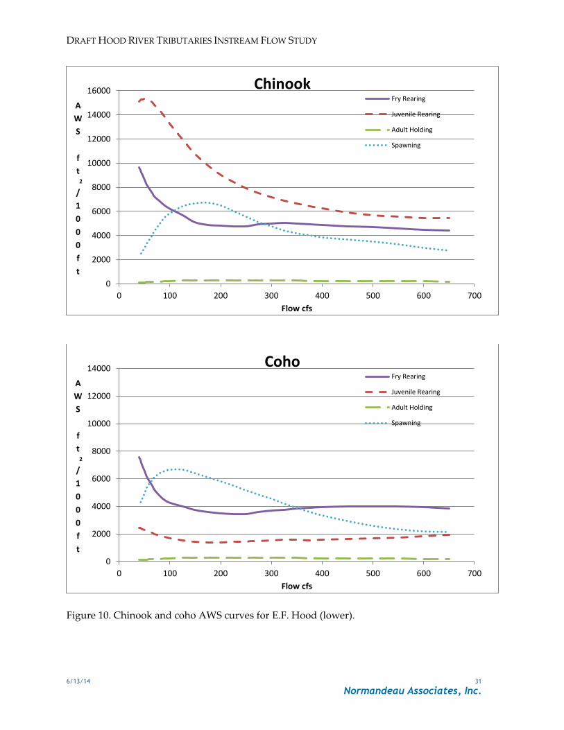
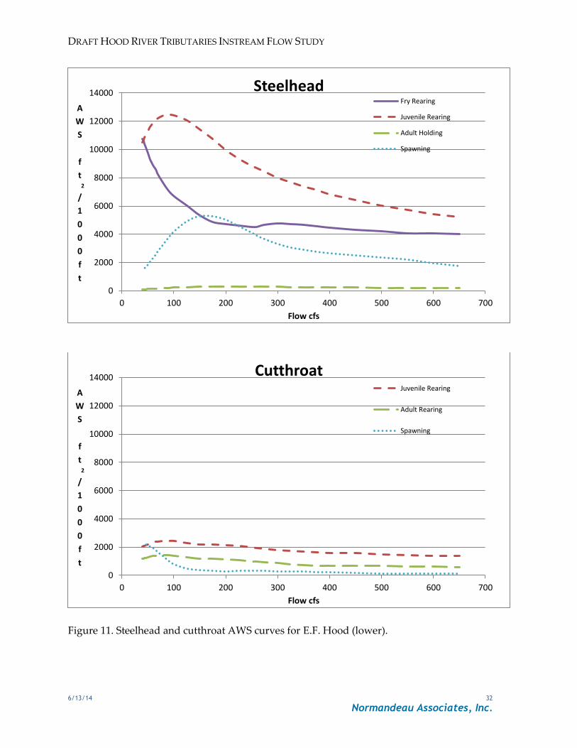
300 cfs. The cutthroat spawning curve shows most suitable habitat at the lowest flows then
declines to 200 cfs before becoming flat (Figures 10-11).
West Fork Hood River
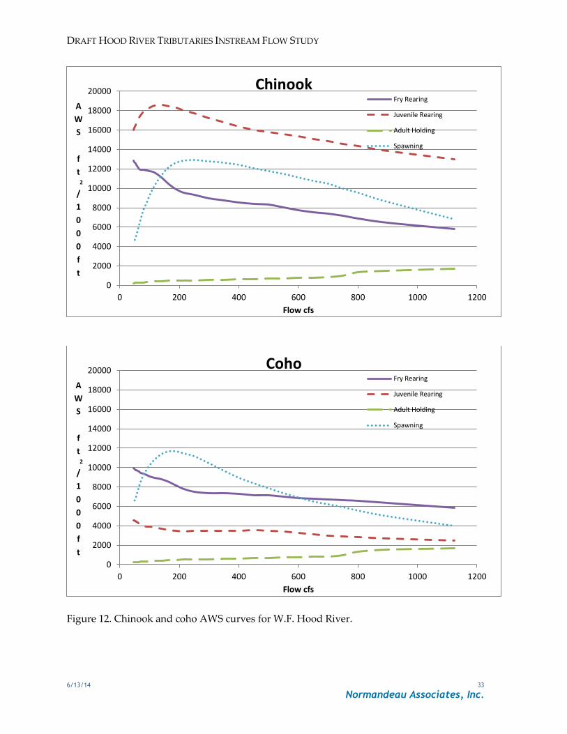
Juvenile rearing AWS varies between species. Chinook curves show maximum suitability for
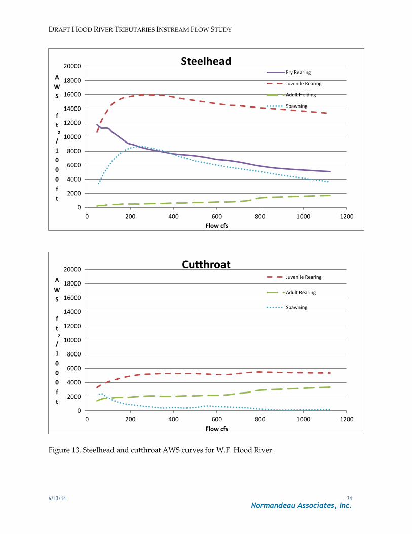
flows between 100 cfs and 350 cfs. Steelhead juvenile rearing increases from low flows, with the
greatest suitability between 200 cfs and 400 cfs, then remain relatively flat. Cutthroat juvenile
and adult trend slightly upward with increasing flows while bull trout juvenile rearing show a
gradual decline and the adult curve is flat. Coho suitability is greatest at low flows then drops
slightly as flows increase, though the curve is essentially flat past 200 cfs. Fry rearing for all
species declines as flows increase.
Spawning AWS curves for Chinook, coho and steelhead are similar with abrupt increases from
low flows to maximum suitability at 200-400 cfs for Chinook, 100-350 cfs for coho and 150-450
cfs for steelhead. Spawning suitability for bull trout and cutthroat is highest at flows less than
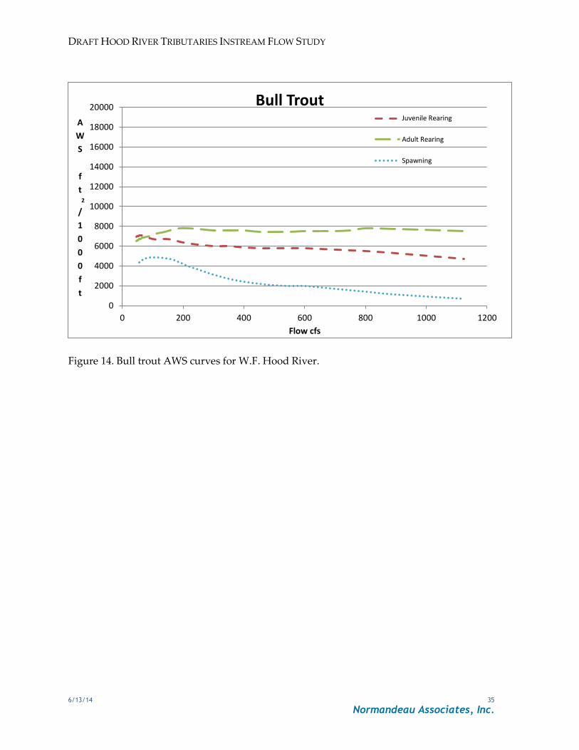
200 cfs, and declines gradually as flow increase (Figures 13-14).
DRAFT HOOD RIVER TRIBUTARIES INSTREAM FLOW STUDY
6/13/14 25
Normandeau Associates, Inc.
Figure 4. Chinook and coho AWS curves for Green Point Creek.
0
2000
4000
6000
8000
10000
12000
14000
0 100 200 300 400 500 600
A
W
S
f
t2
/
1
0
0
0
f
t
Flow cfs
Chinook Fry Rearing
Juvenile Rearing
Adult Holding
Spawning
0
2000
4000
6000
8000
10000
12000
14000
0 100 200 300 400 500 600
A
W
S
f
t2
/
1
0
0
0
f
t
Flow cfs
Coho Fry Rearing
Juvenile Rearing
Adult Holding
Spawning

DRAFT HOOD RIVER TRIBUTARIES INSTREAM FLOW STUDY
6/13/14 26
Normandeau Associates, Inc.
Figure 5. Steelhead and cutthroat AWS curves for Green Point Creek.
0
2000
4000
6000
8000
10000
12000
14000
0 100 200 300 400 500 600
A
W
S
f
t2
/
1
0
0
0
f
t
Flow cfs
Steelhead Fry Rearing
Juvenile Rearing
Adult Holding
Spawning
0
2000
4000
6000
8000
10000
12000
14000
0 100 200 300 400 500 600
A
W
S
f
t2
/
1
0
0
0
f
t
Flow cfs
Cutthroat Juvenile Rearing
Adult Rearing
Spawning
DRAFT HOOD RIVER TRIBUTARIES INSTREAM FLOW STUDY
6/13/14 27
Normandeau Associates, Inc.
Figure 6. Steelhead and coho AWS curves for Neal Creek.
0
1000
2000
3000
4000
5000
6000
7000
8000
9000
10000
0 10 20 30 40 50 60 70 80
A
W
S
f
t2
/
1
0
0
0
f
t
Flow cfs
Coho
Fry Rearing
Juvenile Rearing
Adult Holding
Spawning
0
1000
2000
3000
4000
5000
6000
7000
8000
9000
10000
0 10 20 30 40 50 60 70 80
A
W
S
f
t2
/
1
0
0
0
f
t
Flow cfs
Steelhead Fry Rearing
Juvenile Rearing
Adult Holding
Spawning
DRAFT HOOD RIVER TRIBUTARIES INSTREAM FLOW STUDY
6/13/14 28
Normandeau Associates, Inc.
Figure 7. Cutthroat AWS curves for Neal Creek.
0
1000
2000
3000
4000
5000
6000
7000
8000
9000
10000
0 10 20 30 40 50 60 70 80
A
W
S
f
t2
/
1
0
0
0
f
t
Flow cfs
Cutthroat Juvenile Rearing
Adult Rearing
Spawning

DRAFT HOOD RIVER TRIBUTARIES INSTREAM FLOW STUDY
6/13/14 29
Normandeau Associates, Inc.
Figure 8. Chinook and coho AWS curves for E.F. Hood (upper).
0
2000
4000
6000
8000
10000
12000
14000
0 100 200 300 400 500 600 700 800 900 1000
A
W
S
f
t2
/
1
0
0
0
f
t
Flow cfs
Chinook Fry Rearing
Juvenile Rearing
Adult Holding
Spawning
0
2000
4000
6000
8000
10000
12000
14000
0 100 200 300 400 500 600 700 800 900 1000
A
W
S
f
t2
/
1
0
0
0
f
t
Flow cfs
Coho Fry Rearing
Juvenile Rearing
Adult Holding
Spawning
DRAFT HOOD RIVER TRIBUTARIES INSTREAM FLOW STUDY
6/13/14 30
Normandeau Associates, Inc.
Figure 9. Steelhead and cutthroat AWS curves for E.F. Hood (upper).
0
2000
4000
6000
8000
10000
12000
14000
0 100 200 300 400 500 600 700 800 900 1000
A
W
S
f
t2
/
1
0
0
0
f
t
Flow cfs
Steelhead Fry Rearing
Juvenile Rearing
Adult Holding
Spawning
0
2000
4000
6000
8000
10000
12000
14000
0 100 200 300 400 500 600 700 800 900 1000
A
W
S
f
t2
/
1
0
0
0
f
t
Flow cfs
Cutthroat Juvenile Rearing
Adult Rearing
Spawning
DRAFT HOOD RIVER TRIBUTARIES INSTREAM FLOW STUDY
6/13/14 31
Normandeau Associates, Inc.
Figure 10. Chinook and coho AWS curves for E.F. Hood (lower).
0
2000
4000
6000
8000
10000
12000
14000
16000
0 100 200 300 400 500 600 700
A
W
S
f
t2
/
1
0
0
0
f
t
Flow cfs
Chinook Fry Rearing
Juvenile Rearing
Adult Holding
Spawning
0
2000
4000
6000
8000
10000
12000
14000
0 100 200 300 400 500 600 700
A
W
S
f
t2
/
1
0
0
0
f
t
Flow cfs
Coho Fry Rearing
Juvenile Rearing
Adult Holding
Spawning
DRAFT HOOD RIVER TRIBUTARIES INSTREAM FLOW STUDY
6/13/14 32
Normandeau Associates, Inc.
Figure 11. Steelhead and cutthroat AWS curves for E.F. Hood (lower).
0
2000
4000
6000
8000
10000
12000
14000
0 100 200 300 400 500 600 700
A
W
S
f
t2
/
1
0
0
0
f
t
Flow cfs
Steelhead Fry Rearing
Juvenile Rearing
Adult Holding
Spawning
0
2000
4000
6000
8000
10000
12000
14000
0 100 200 300 400 500 600 700
A
W
S
f
t2
/
1
0
0
0
f
t
Flow cfs
Cutthroat Juvenile Rearing
Adult Rearing
Spawning
DRAFT HOOD RIVER TRIBUTARIES INSTREAM FLOW STUDY
6/13/14 33
Normandeau Associates, Inc.
Figure 12. Chinook and coho AWS curves for W.F. Hood River.
0
2000
4000
6000
8000
10000
12000
14000
16000
18000
20000
0 200 400 600 800 1000 1200
A
W
S
f
t2
/
1
0
0
0
f
t
Flow cfs
Chinook Fry Rearing
Juvenile Rearing
Adult Holding
Spawning
0
2000
4000
6000
8000
10000
12000
14000
16000
18000
20000
0 200 400 600 800 1000 1200
A
W
S
f
t2
/
1
0
0
0
f
t
Flow cfs
Coho Fry Rearing
Juvenile Rearing
Adult Holding
Spawning
DRAFT HOOD RIVER TRIBUTARIES INSTREAM FLOW STUDY
6/13/14 34
Normandeau Associates, Inc.
Figure 13. Steelhead and cutthroat AWS curves for W.F. Hood River.
0
2000
4000
6000
8000
10000
12000
14000
16000
18000
20000
0 200 400 600 800 1000 1200
A
W
S
f
t2
/
1
0
0
0
f
t
Flow cfs
Steelhead Fry Rearing
Juvenile Rearing
Adult Holding
Spawning
0
2000
4000
6000
8000
10000
12000
14000
16000
18000
20000
0 200 400 600 800 1000 1200
A
W
S
f
t2
/
1
0
0
0
f
t
Flow cfs
Cutthroat Juvenile Rearing
Adult Rearing
Spawning
DRAFT HOOD RIVER TRIBUTARIES INSTREAM FLOW STUDY
6/13/14 35
Normandeau Associates, Inc.
Figure 14. Bull trout AWS curves for W.F. Hood River.
0
2000
4000
6000
8000
10000
12000
14000
16000
18000
20000
0 200 400 600 800 1000 1200
A
W
S
f
t2
/
1
0
0
0
f
t
Flow cfs
Bull Trout Juvenile Rearing
Adult Rearing
Spawning
DRAFT HOOD RIVER TRIBUTARIES INSTREAM FLOW STUDY
6/13/14 36
Normandeau Associates, Inc.
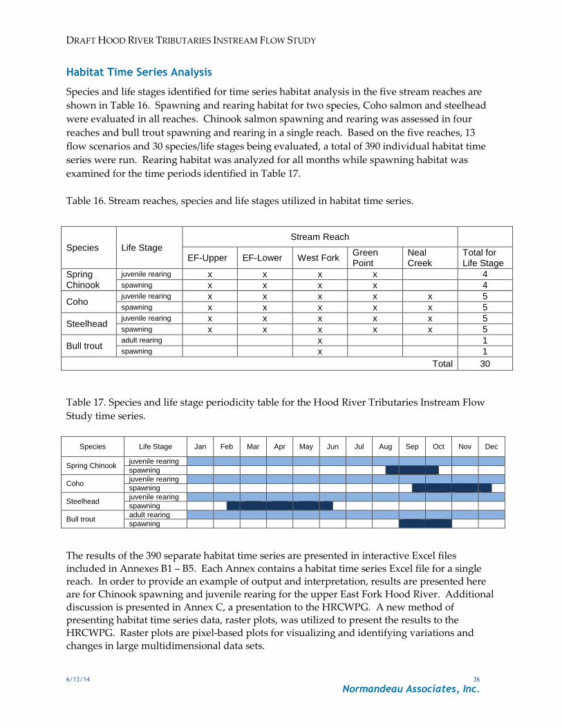
Habitat Time Series Analysis
Species and life stages identified for time series habitat analysis in the five stream reaches are
shown in Table 16. Spawning and rearing habitat for two species, Coho salmon and steelhead
were evaluated in all reaches. Chinook salmon spawning and rearing was assessed in four
reaches and bull trout spawning and rearing in a single reach. Based on the five reaches, 13
flow scenarios and 30 species/life stages being evaluated, a total of 390 individual habitat time
series were run. Rearing habitat was analyzed for all months while spawning habitat was
examined for the time periods identified in Table 17.
Table 16. Stream reaches, species and life stages utilized in habitat time series.
Species Life Stage
Stream Reach
EF-Upper EF-Lower West Fork Green Point
Neal Creek
Total for Life Stage
Spring Chinook
juvenile rearing x x x x 4 spawning x x x x 4
Coho juvenile rearing x x x x x 5 spawning x x x x x 5
Steelhead juvenile rearing x x x x x 5 spawning x x x x x 5
Bull trout adult rearing x 1 spawning x 1
Total 30
Table 17. Species and life stage periodicity table for the Hood River Tributaries Instream Flow
Study time series.
Species Life Stage Jan Feb Mar Apr May Jun Jul Aug Sep Oct Nov Dec
Spring Chinook juvenile rearing
spawning
Coho juvenile rearing
spawning
Steelhead juvenile rearing
spawning
Bull trout adult rearing
spawning
The results of the 390 separate habitat time series are presented in interactive Excel files
included in Annexes B1 – B5. Each Annex contains a habitat time series Excel file for a single reach. In order to provide an example of output and interpretation, results are presented here
are for Chinook spawning and juvenile rearing for the upper East Fork Hood River. Additional
discussion is presented in Annex C, a presentation to the HRCWPG. A new method of presenting habitat time series data, raster plots, was utilized to present the results to the
HRCWPG. Raster plots are pixel-based plots for visualizing and identifying variations and
changes in large multidimensional data sets.
DRAFT HOOD RIVER TRIBUTARIES INSTREAM FLOW STUDY
6/13/14 37
Normandeau Associates, Inc.
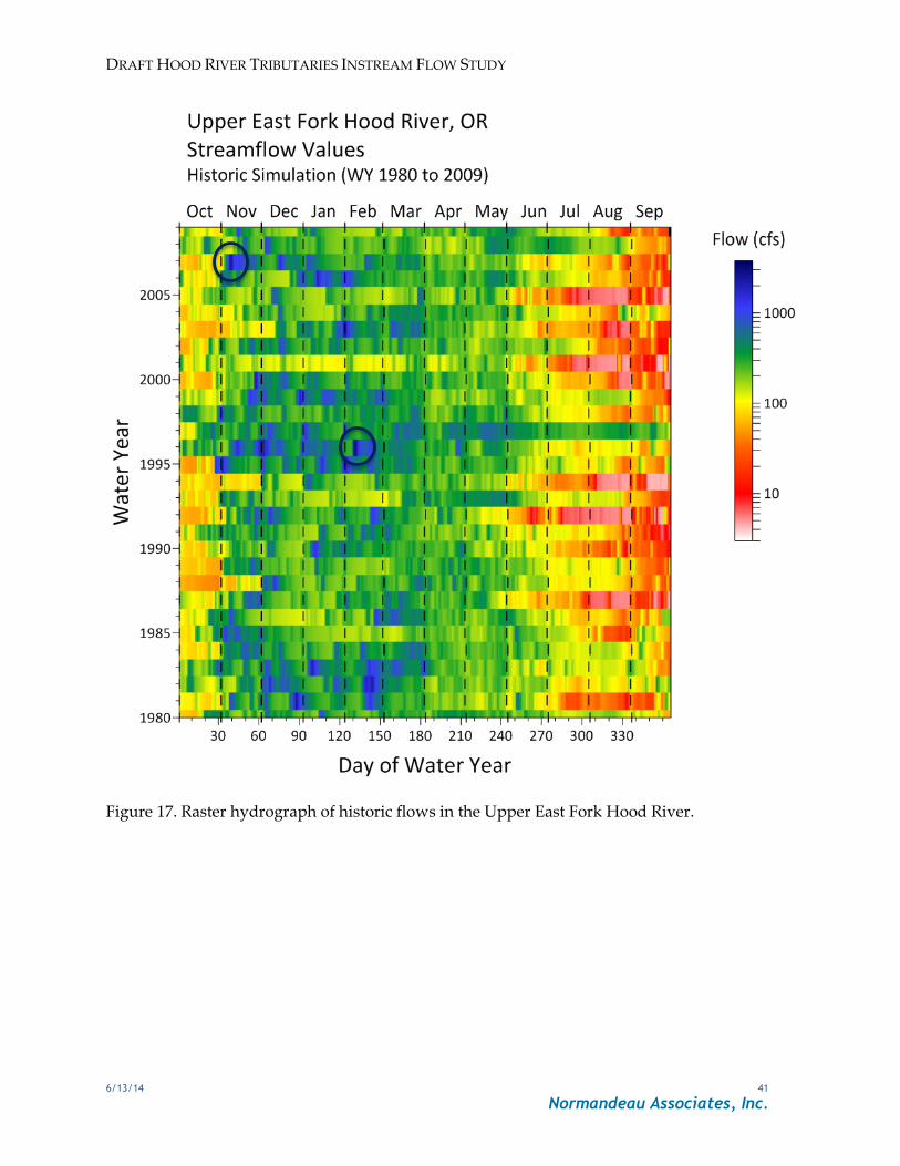
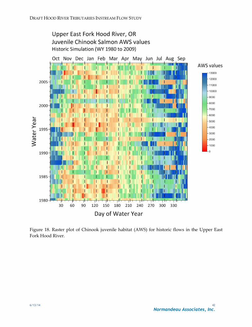
Originally developed by Keim (2000) they were first applied in hydrology by Koehler (2004) as a means of highlighting inter-annual and intra-annual changes in streamflow. The raster hydrographs in WaterWatch (http://waterwatch.usgs.gov/?id=wwchart_rastergraph), like those
developed by Koehler, depict years on the y-axis and days along the x-axis.
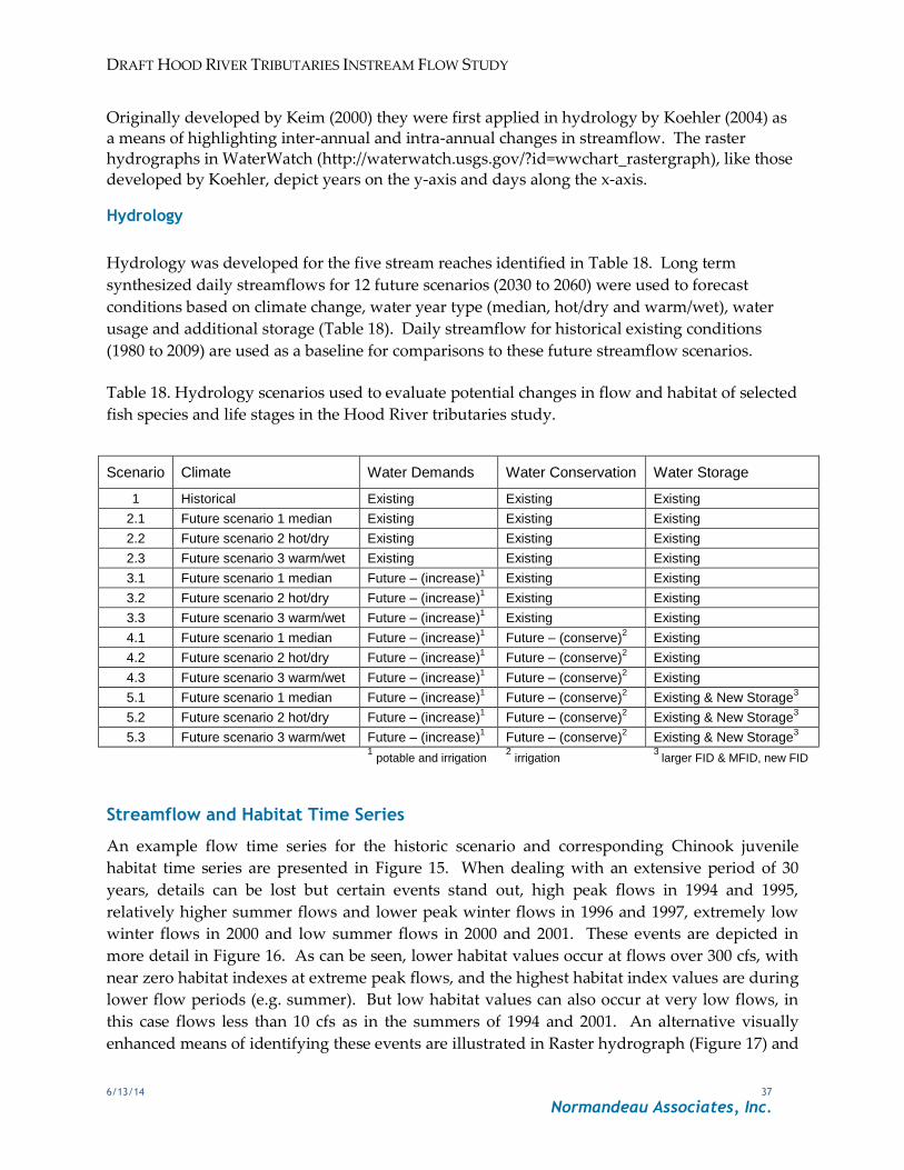
Hydrology
Hydrology was developed for the five stream reaches identified in Table 18. Long term
synthesized daily streamflows for 12 future scenarios (2030 to 2060) were used to forecast
conditions based on climate change, water year type (median, hot/dry and warm/wet), water
usage and additional storage (Table 18). Daily streamflow for historical existing conditions
(1980 to 2009) are used as a baseline for comparisons to these future streamflow scenarios.
Table 18. Hydrology scenarios used to evaluate potential changes in flow and habitat of selected
fish species and life stages in the Hood River tributaries study.
Scenario Climate Water Demands Water Conservation Water Storage
1 Historical Existing Existing Existing
2.1 Future scenario 1 median Existing Existing Existing
2.2 Future scenario 2 hot/dry Existing Existing Existing
2.3 Future scenario 3 warm/wet Existing Existing Existing
3.1 Future scenario 1 median Future – (increase)1 Existing Existing
3.2 Future scenario 2 hot/dry Future – (increase)1 Existing Existing
3.3 Future scenario 3 warm/wet Future – (increase)1 Existing Existing
4.1 Future scenario 1 median Future – (increase)1 Future – (conserve)
2 Existing
4.2 Future scenario 2 hot/dry Future – (increase)1 Future – (conserve)
2 Existing
4.3 Future scenario 3 warm/wet Future – (increase)1 Future – (conserve)
2 Existing
5.1 Future scenario 1 median Future – (increase)1 Future – (conserve)
2 Existing & New Storage3
5.2 Future scenario 2 hot/dry Future – (increase)1 Future – (conserve)
2 Existing & New Storage3
5.3 Future scenario 3 warm/wet Future – (increase)1 Future – (conserve)
2 Existing & New Storage3
1 potable and irrigation
2 irrigation
3 larger FID & MFID, new FID
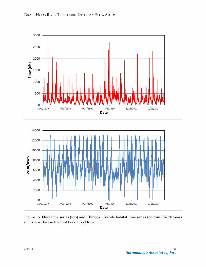
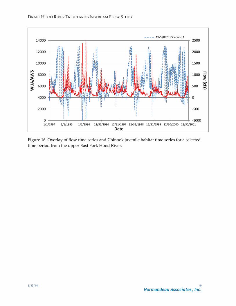
Streamflow and Habitat Time Series
An example flow time series for the historic scenario and corresponding Chinook juvenile
habitat time series are presented in Figure 15. When dealing with an extensive period of 30
years, details can be lost but certain events stand out, high peak flows in 1994 and 1995,
relatively higher summer flows and lower peak winter flows in 1996 and 1997, extremely low
winter flows in 2000 and low summer flows in 2000 and 2001. These events are depicted in
more detail in Figure 16. As can be seen, lower habitat values occur at flows over 300 cfs, with
near zero habitat indexes at extreme peak flows, and the highest habitat index values are during
lower flow periods (e.g. summer). But low habitat values can also occur at very low flows, in
this case flows less than 10 cfs as in the summers of 1994 and 2001. An alternative visually
enhanced means of identifying these events are illustrated in Raster hydrograph (Figure 17) and

DRAFT HOOD RIVER TRIBUTARIES INSTREAM FLOW STUDY
6/13/14 38
Normandeau Associates, Inc.
habitat (Figure 18) plots. The high flows of February 1996 and November of 2006 are easily
identified in Figure 17.
By examining the relationship between flow and habitat for Chinook juvenile, the basis for
these events becomes apparent (Figure 19). From the peak of the curve to an inflection point
around 300 cfs, AWS is relatively high. Past this point AWS gradually decreases. Similarly
AWS is relatively high at the low end of the curve before its drops precipitously at flows less
than 10 cfs.
DRAFT HOOD RIVER TRIBUTARIES INSTREAM FLOW STUDY
6/13/14 39
Normandeau Associates, Inc.
Figure 15. Flow time series (top) and Chinook juvenile habitat time series (bottom) for 30 years
of historic flow in the East Fork Hood River..
0
500
1000
1500
2000
2500
3000
10/1/1979 3/23/1985 9/13/1990 3/5/1996 8/26/2001 2/16/2007
Flo
w (
cfs)
Date
0
2000
4000
6000
8000
10000
12000
14000
10/1/1979 3/23/1985 9/13/1990 3/5/1996 8/26/2001 2/16/2007
WU
A/A
WS
Date
DRAFT HOOD RIVER TRIBUTARIES INSTREAM FLOW STUDY
6/13/14 40
Normandeau Associates, Inc.
Figure 16. Overlay of flow time series and Chinook juvenile habitat time series for a selected
time period from the upper East Fork Hood River.
-1000
-500
0
500
1000
1500
2000
2500
0
2000
4000
6000
8000
10000
12000
14000
1/1/1994 1/1/1995 1/1/1996 12/31/1996 12/31/1997 12/31/1998 12/31/1999 12/30/2000 12/30/2001
Flow
(cfs) WU
A/A
WS
Date
AWS (ft2⁄ft) Scenario 1
DRAFT HOOD RIVER TRIBUTARIES INSTREAM FLOW STUDY
6/13/14 41
Normandeau Associates, Inc.
Figure 17. Raster hydrograph of historic flows in the Upper East Fork Hood River.
DRAFT HOOD RIVER TRIBUTARIES INSTREAM FLOW STUDY
6/13/14 42
Normandeau Associates, Inc.
Figure 18. Raster plot of Chinook juvenile habitat (AWS) for historic flows in the Upper East
Fork Hood River.

DRAFT HOOD RIVER TRIBUTARIES INSTREAM FLOW STUDY
6/13/14 43
Normandeau Associates, Inc.
Figure 19. Chinook juvenile WUA/AWS curve for the upper East Fork Hood River.
Flow and Habitat Duration
Flow duration curves provide a means to compare different flow regimes with respect to the
amount of time certain flow levels occur. For the upper East Fork Hood River graphs are
provided that depict flow exceedance from 0-100 % and 5-95 % for the period of record (Figure
20). Future hydrology for all scenarios shows an increase in high flows and somewhat lower
low flows for most of the scenarios compared to historical. Examination of Chinook juvenile
habitat duration curves shows slightly more habitat 25% of the time and slightly less 50% of the
time for all future scenarios over historical (Figure 21). Because it has been shown that both
high flows and very low flows can lower the habitat index, this follows what is shown in the
flow duration curve.
Flow duration curves for spring Chinook spawning cover a short period of time (August 15 to
October 15) and flows exceed 250 cfs just 5% of the time (Figure 22). Future flow scenarios
based on climate change (2.1-2.3) and water demand (3.1-3.2) display lower flows than historical all the time. Scenarios based on water conservation and storage exhibit higher high flows, but
also greater low flows. The overall lower flows under climate change and water demand
scenarios result in a reduction of spawning habitat (Figure 22). Under water conservation and storage scenarios spawning habitat is greater for approximately 50% of the time for scenarios
4.1 and 4.2, and most of the time for scenarios with water storage incorporated.
0
2000
4000
6000
8000
10000
12000
14000
0 100 200 300 400 500 600 700 800 900
WU
A/A
WS
Flow (cfs)
Chinook Juvenile Rearing AWS
Simulated
Projected
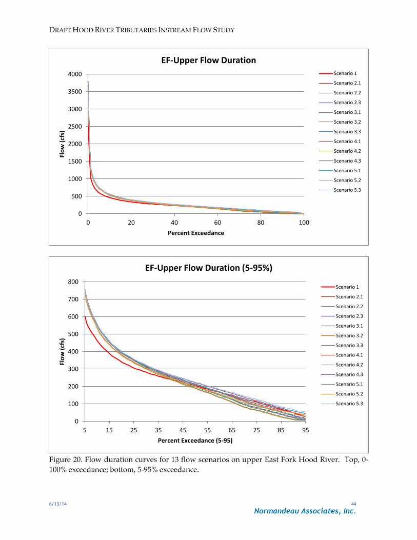
DRAFT HOOD RIVER TRIBUTARIES INSTREAM FLOW STUDY
6/13/14 44
Normandeau Associates, Inc.
Figure 20. Flow duration curves for 13 flow scenarios on upper East Fork Hood River. Top, 0-
100% exceedance; bottom, 5-95% exceedance.
0
500
1000
1500
2000
2500
3000
3500
4000
0 20 40 60 80 100
Flo
w (
cfs)
Percent Exceedance
EF-Upper Flow Duration Scenario 1
Scenario 2.1
Scenario 2.2
Scenario 2.3
Scenario 3.1
Scenario 3.2
Scenario 3.3
Scenario 4.1
Scenario 4.2
Scenario 4.3
Scenario 5.1
Scenario 5.2
Scenario 5.3
0
100
200
300
400
500
600
700
800
5 15 25 35 45 55 65 75 85 95
Flo
w (
cfs)
Percent Exceedance (5-95)
EF-Upper Flow Duration (5-95%)
Scenario 1
Scenario 2.1
Scenario 2.2
Scenario 2.3
Scenario 3.1
Scenario 3.2
Scenario 3.3
Scenario 4.1
Scenario 4.2
Scenario 4.3
Scenario 5.1
Scenario 5.2
Scenario 5.3
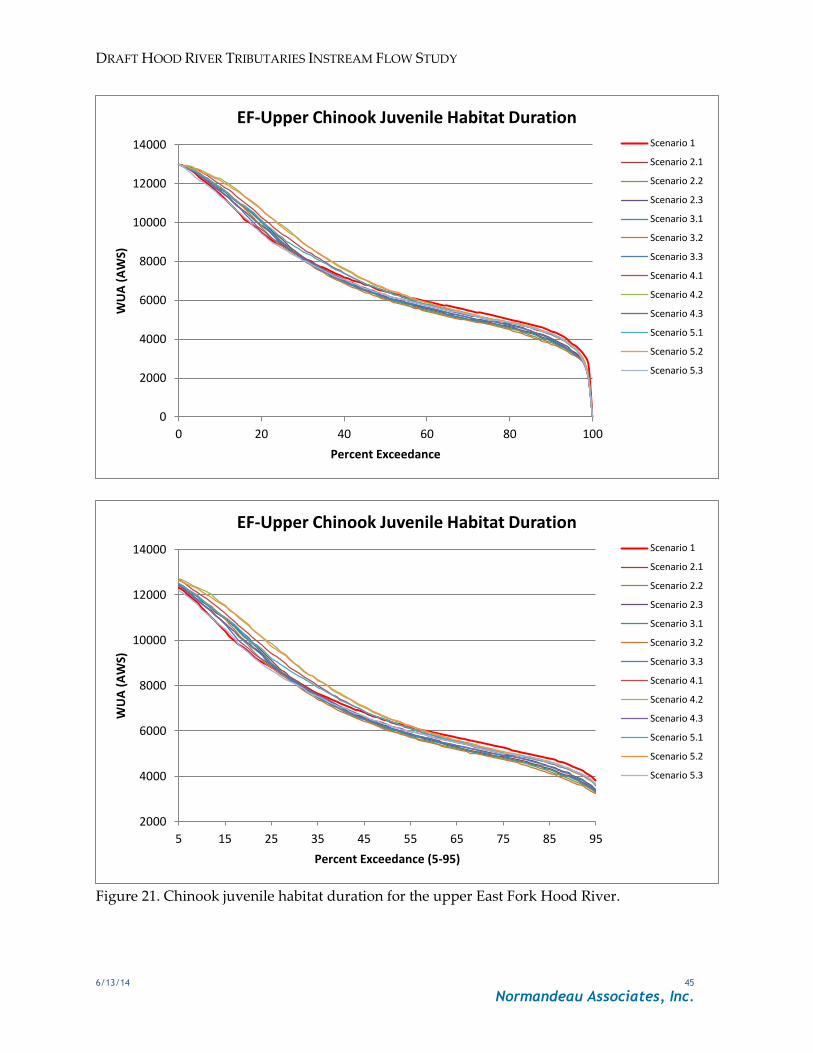
DRAFT HOOD RIVER TRIBUTARIES INSTREAM FLOW STUDY
6/13/14 45
Normandeau Associates, Inc.
Figure 21. Chinook juvenile habitat duration for the upper East Fork Hood River.
0
2000
4000
6000
8000
10000
12000
14000
0 20 40 60 80 100
WU
A (
AW
S)
Percent Exceedance
EF-Upper Chinook Juvenile Habitat Duration Scenario 1
Scenario 2.1
Scenario 2.2
Scenario 2.3
Scenario 3.1
Scenario 3.2
Scenario 3.3
Scenario 4.1
Scenario 4.2
Scenario 4.3
Scenario 5.1
Scenario 5.2
Scenario 5.3
2000
4000
6000
8000
10000
12000
14000
5 15 25 35 45 55 65 75 85 95
WU
A (
AW
S)
Percent Exceedance (5-95)
EF-Upper Chinook Juvenile Habitat Duration Scenario 1
Scenario 2.1
Scenario 2.2
Scenario 2.3
Scenario 3.1
Scenario 3.2
Scenario 3.3
Scenario 4.1
Scenario 4.2
Scenario 4.3
Scenario 5.1
Scenario 5.2
Scenario 5.3
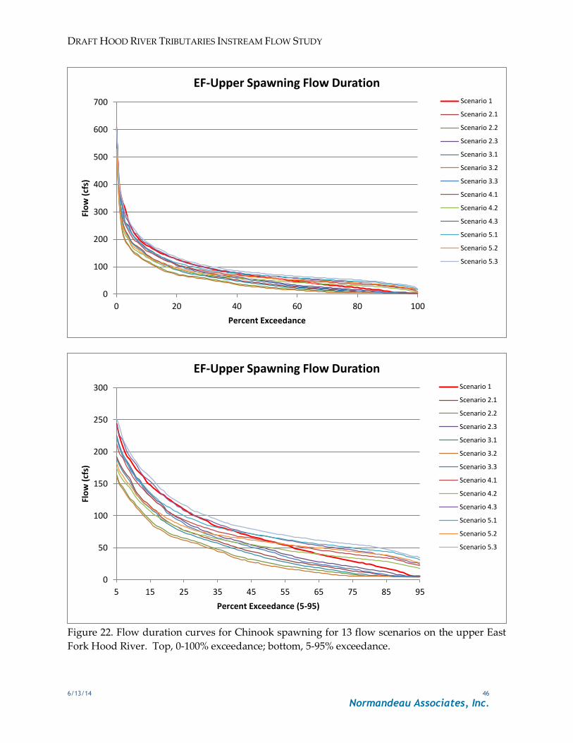
DRAFT HOOD RIVER TRIBUTARIES INSTREAM FLOW STUDY
6/13/14 46
Normandeau Associates, Inc.
Figure 22. Flow duration curves for Chinook spawning for 13 flow scenarios on the upper East
Fork Hood River. Top, 0-100% exceedance; bottom, 5-95% exceedance.
0
100
200
300
400
500
600
700
0 20 40 60 80 100
Flo
w (
cfs)
Percent Exceedance
EF-Upper Spawning Flow Duration Scenario 1
Scenario 2.1
Scenario 2.2
Scenario 2.3
Scenario 3.1
Scenario 3.2
Scenario 3.3
Scenario 4.1
Scenario 4.2
Scenario 4.3
Scenario 5.1
Scenario 5.2
Scenario 5.3
0
50
100
150
200
250
300
5 15 25 35 45 55 65 75 85 95
Flo
w (
cfs)
Percent Exceedance (5-95)
EF-Upper Spawning Flow Duration Scenario 1
Scenario 2.1
Scenario 2.2
Scenario 2.3
Scenario 3.1
Scenario 3.2
Scenario 3.3
Scenario 4.1
Scenario 4.2
Scenario 4.3
Scenario 5.1
Scenario 5.2
Scenario 5.3

DRAFT HOOD RIVER TRIBUTARIES INSTREAM FLOW STUDY
6/13/14 47
Normandeau Associates, Inc.
Figure 23. Chinook spawning habitat duration for the upper East Fork Hood River.
0
2000
4000
6000
8000
10000
12000
0 20 40 60 80 100
WU
A (
AW
S)
Percent Exceedance
EF-Upper Chinook Spawning Habitat Duration Scenario 1
Scenario 2.1
Scenario 2.2
Scenario 2.3
Scenario 3.1
Scenario 3.2
Scenario 3.3
Scenario 4.1
Scenario 4.2
Scenario 4.3
Scenario 5.1
Scenario 5.2
Scenario 5.3
0
2000
4000
6000
8000
10000
12000
5 15 25 35 45 55 65 75 85 95
WU
A (
AW
S)
Percent Exceedance (5-95)
EF-Upper Chinook Spawning Habitat Duration Scenario 1
Scenario 2.1
Scenario 2.2
Scenario 2.3
Scenario 3.1
Scenario 3.2
Scenario 3.3
Scenario 4.1
Scenario 4.2
Scenario 4.3
Scenario 5.1
Scenario 5.2
Scenario 5.3
DRAFT HOOD RIVER TRIBUTARIES INSTREAM FLOW STUDY
6/13/14 48
Normandeau Associates, Inc.
Discussion
Although we are reporting on all four streams in a single report, there are four separate
instream flow studies; one each for Green Point Creek, Neal Creek, East Fork Hood River, and
West Fork Hood River. Even though all four streams are tributaries of the Hood River in the same vicinity, they vary in size and respond differently to hydrologic events. This became
painfully evident when we mobilized for the field work targeting the calibration flows.
Subsequent to a rain event after which we hoped to measure high flow data, both the East and West Forks responded and became torrents, Green Point Creek responded moderately, and
Neal Creek flow barely increased. Of course the elevation, size, and orientation of each
watershed are responsible for the different hydrologic responses to the same rain event. Likewise, the hydraulic habitat characterized by each instream flow study will vary differently
in response climatic induced changes in flow.
There is one conclusion common to all streams: the hydraulic habitat index, AWS, indicates low habitat suitability for adult holding in all reaches for all reasonable flows. Low, flat AWS curves
indicate that changes in flow have little influence on adult holding habitat. Deep habitats are
scarce. If feasible, restoration of holding habitat would have more influence on the availability than changes in flow.
A controversial indication of the AWS/flow relationship for adult and juvenile salmonids in the
East Fork is the favourability of low flows (Annex A1 and D). This resulted in changing the Chinook spawning HSC for the larger East and West Forks from the MFID HSC to the WDFW
River HSC. It was noted early in the HSC discussion (Annex A) that the MFID Chinook
spawning HSC indicated shallow suitability. Although appropriate for the smaller streams, the shallow suitability was not appropriate for the larger streams. No rational changes could be
made to the juvenile or fry HSC. Analysis of the depth and velocity components of the transect
data show that the East Fork reaches (particularly the Upper site) are shallow and fast limiting suitability at higher flows (Annex A1). Recent channel changes and aggradation may contribute
to this. Expansion of the reaches to include more of the river and additional transects would
will help determine if the AWS/flow relationships are influenced by sites randomly selected.
Instream flow studies rarely answer the question, “What is the best flow?” That question is
answered by balancing biological, social, and economic needs. Even when considering only a
single species, the index of hydraulic habitat for different life-stages will respond differently to changing flow and no one flow will be the best for all life-stages. The results of these instream
flow studies provide tools to assess the biological impacts to hydraulic habitat for the species of
interest in each stream. The primary tools for assessing responses to changing flow are the Excel files in Annexes B1 through B5. Each file contains the results for one study reach. Each
specie/life-stage habitat time series exceedance statistics and habitat duration graphs are
presented in separate worksheets. The habitat duration graphs are presented both as a group of all climate scenarios and as interactive graphs enabling the user to select a scenario to compare
to the historical graph. The user can select any one of the 12 climate altered scenarios to

DRAFT HOOD RIVER TRIBUTARIES INSTREAM FLOW STUDY
6/13/14 49
Normandeau Associates, Inc.
compare with the historical scenario. Each of the graphs are also presented including all
exceedance values (0% to 100%) and the 5% to 95% range of exceedance values. The 5% to 95% graph eliminates the extremes and enables the range scale to be reduced for greater resolution
of the graphs when comparing scenarios.
An overview of the instream flow studies and detailed comparisons of the climate scenarios and habitat time series for Chinook spawning and Chinook juvenile rearing in the Upper East Fork
Reach is presented in Annex C, the final presentation to the HRCWPG. The presentation relies
heavily on raster plots, a new way to visualize the time series data set. In presentation mode, the user can toggle between two comparative raster plots on the same slide and see where and
when changes to the raster hydrograph and hydraulic habitat index occur anywhere in the time
series. Another use of the raster plot is to plot the difference in habitat index values between a climate scenario and the historical record. Figure 24 depicts decreases in Chinook rearing AWS
comparing the future 5.3 climate scenario to the historical record for most of the East Fork Hood
River time series. However, increases in AWS due to scenario 5.3 occur in the summer concurrent with low flow and the lowest habitat values. The increases in habitat values,
although much less frequent, may be of greater biological significance occurring in a potential
habitat bottleneck. This is further demonstrated by Figures 25 and 26. The times when the 50% AWS value (historical) are equalled or exceeded are plotted with a black dot over the raster
hydrograph of the historical (Figure 25) and 5.3 (Figure 26) scenarios. The July through
September low habitat values in the historical scenario (Figure 25) correspond to dry periods without the black dot overlay. Those low AWS values are not existent in the 5.3 scenario
summer (Figure 26).
It is important to note that for a flow prescription in any of these streams, additional habitat mapping and potentially additional transects will be required to determine the applicability of
the AWS/flow relationship to reaches not habitat mapped in this study. Due to available
funding each reach was limited to one mile of stream. Many considerations were included in the reach selection process and reaches that are productive and representative were chosen.
This does not, however, guarantee that each reach will represent the entire stream. Additional
habitat mapping will either verify the representativeness or indicate the need for additional transects.
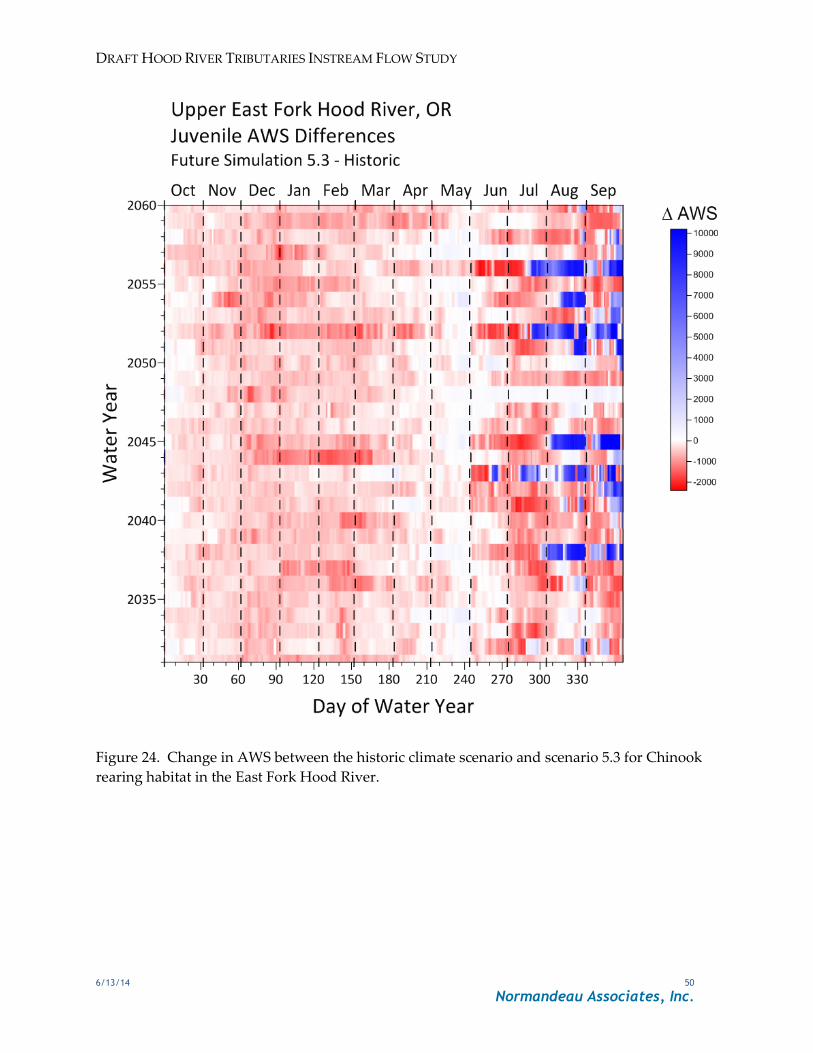
DRAFT HOOD RIVER TRIBUTARIES INSTREAM FLOW STUDY
6/13/14 50
Normandeau Associates, Inc.
Figure 24. Change in AWS between the historic climate scenario and scenario 5.3 for Chinook
rearing habitat in the East Fork Hood River.
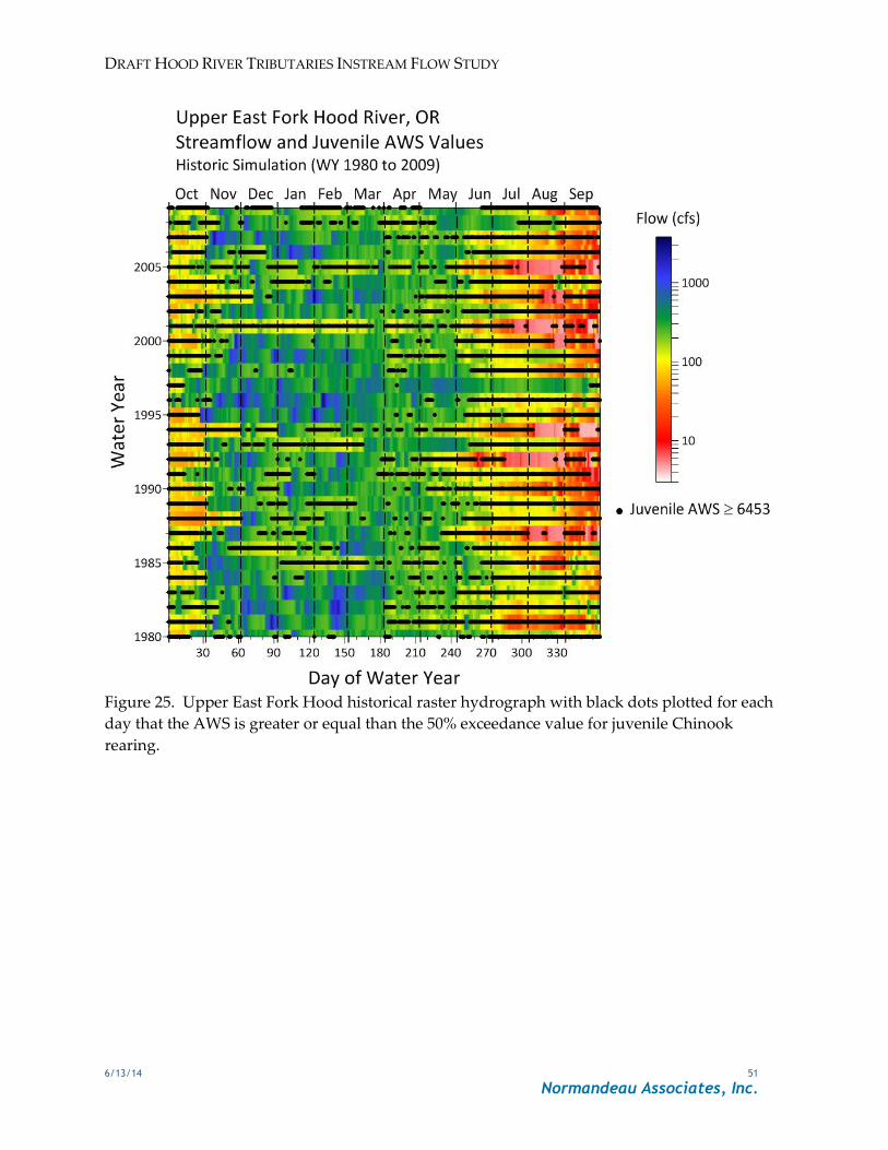
DRAFT HOOD RIVER TRIBUTARIES INSTREAM FLOW STUDY
6/13/14 51
Normandeau Associates, Inc.
Figure 25. Upper East Fork Hood historical raster hydrograph with black dots plotted for each
day that the AWS is greater or equal than the 50% exceedance value for juvenile Chinook
rearing.
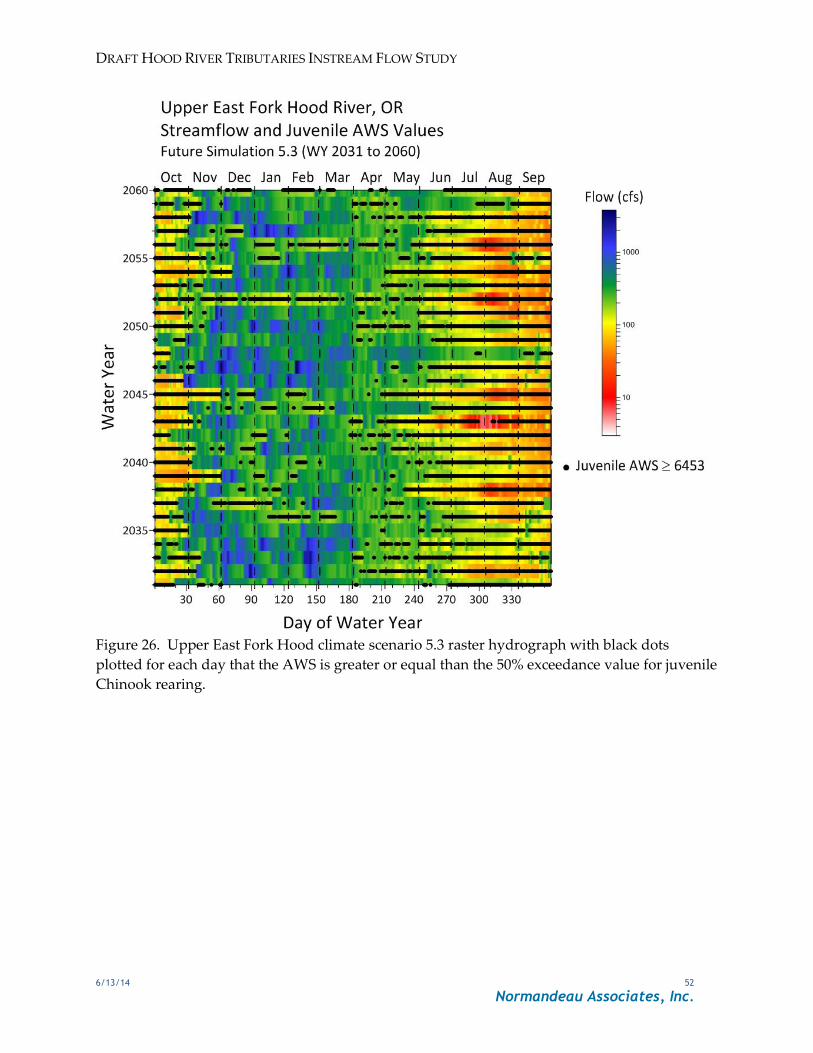
DRAFT HOOD RIVER TRIBUTARIES INSTREAM FLOW STUDY
6/13/14 52
Normandeau Associates, Inc.
Figure 26. Upper East Fork Hood climate scenario 5.3 raster hydrograph with black dots
plotted for each day that the AWS is greater or equal than the 50% exceedance value for juvenile
Chinook rearing.
DRAFT HOOD RIVER TRIBUTARIES INSTREAM FLOW STUDY
6/13/14 53
Normandeau Associates, Inc.
References
Bovee, K.D. 1997. Data collection procedures for the Physical Habitat Simulation System.
USGS Biological Resources Division, Ft. Collins, CO. 141 pp.
Bovee, K.D., B.L. Lamb, J.M. Bartholow, C.B. Stalnaker, J. Taylor, and J. Henriksen. 1998. Stream habitat analysis using the instream flow incremental methodology. USGS
Biological Resources Division Information and Technology Report USGS/BRD-1998-
0004. viii + 131 pp.
Bovee, K.D., and R.T. Milhous. 1978. Hydraulic simulation in instream flow studies: theory
and techniques. Instream Flow Information Paper 5. United States Fish and Wildlife
Service FWS/OBS-78/33. 129pp.
Bovee, K.D., and J.R. Zuboy, editors. 1988. Proceedings of a workshop on the development and
evaluation of habitat suitability criteria. United States Fish and Wildlife Service,
Biological Report 88(11). 407pp.
Bremm, D.J. 1988. Comparison of stream velocity simulations for the IFG-4 model three-flow,
one-flow, and no-velocity options. M.S. Thesis, Humboldt State University. Arcata,
California. 54pp.
Jowett, I.G., T.R. Payne, and R.T. Milhous. 2014. SEFA System for Environmental Flow
Analysis Software Manual, Version 1.21, February 2014. 226pp.
Keim, D.A. 2000. Designing pixel-oriented visualization techniques: theory and applications. IEEE Transactions on Visualization and Computer Graphics, 6(1), 59-78.
Koehler, R. 2004. Raster Based Analysis and Visualization of Hydrologic Time Series. Ph.D.
dissertation, University of Arizona. Tucson, AZ, 189 p.
Milhous, R.T., D.L. Wegner, and T. Waddle. 1984. User's guide to the Physical Habitat
Simulation System (PHABSIM). Instream Flow Information Paper 11. United States
Fish and Wildlife Service Report FWS/OBS-81/43.
Morhardt, J.E., D.F. Hanson, and P.J. Coulston. 1983. Instream flow: improved accuracy
through habitat mapping. In Waterpower ’83: International Conference on Hydropower
(Vol III, pp 1294-1304). September 1983, Knoxville, Tennessee.
Rantz, S.E. 1982. Measurement and computation of streamflow: Volume 1. Measurements of
stage and discharge. United States Geological Survey Water Supply Paper 2175. 284pp.
Trihey, E.W., and D.L. Wegner. 1981. Field data collection for use with the Physical Habitat Simulation system of the Instream Flow Group. United States Fish and Wildlife Service
Report. 151pp.
Oregon Department of Fish and Wildlife. 2010. Aquatic Inventories Project, Methods for Stream Habitat Surveys. Conservation and Recovery Program, Corvallis, OR. 70pp.

DRAFT HOOD RIVER TRIBUTARIES INSTREAM FLOW STUDY
6/13/14 54
Normandeau Associates, Inc.
Payne, T.R. 1987. One-flow IFG-4 - what it is and how it works. Instream Flow Chronicle
4(1):1-2. Colorado State University, Fort Collins, Colorado.
Payne, T.R. 1988a. A comparison of weighted usable area calculations using four variations of
the IFG4 hydraulic model. Paper presented at AFS Bioengineering Symposium, October
24-27, 1988, Portland, Oregon.
Payne, T.R. 1988b. PHABSIM analytical errors and implications for IFIM. Instream Flow
Chronicle, Vol. V, No. 3. Ft. Collins, CO.
Payne, T.R. 1992. Stratified random selection process for the placement of Physical Habitat Simulation (PHABSIM) transects. Paper presented at AFS Western Division Meeting,
July 13-16, 1992, Fort Collins, Colorado.

DRAFT HOOD RIVER TRIBUTARIES INSTREAM FLOW STUDY
6/13/14 55
Normandeau Associates, Inc.
Appendix A: Habitat Mapping
Appendix B: Transect Profiles, and Calibration Flow Velocities and Water Surface Elevations
Appendix C: PHABSIM Calibration Summaries
Appendix D: Simulated Water Surface Elevations and Velocities
Appendix E: Tabular AWS Values