Homomorphic Training of 30,000 LogisticRegression Models

Flavio Bergamaschi1, Shai Halevi2, Tzipora T. Halevi3, and Hamish Hunt1

1 IBM Research, UK, {flavio,hamishhun}@uk.ibm.com2 IBM Research, NY, USA, shaih@alum.mit.edu3 Brooklyn College, NY, USA, thalevi@nyu.edu

Abstract. In this work, we demonstrate the use the CKKS homomor-phic encryption scheme to train a large number of logistic regressionmodels simultaneously, as needed to run a genome-wide association study(GWAS) on encrypted data. Our implementation can train more than30,000 models (each with four features) in about 20 minutes. To thatend, we rely on a similar iterative Nesterov procedure to what was usedby Kim, Song, Kim, Lee, and Cheon to train a single model [14]. Weadapt this method to train many models simultaneously using the SIMDcapabilities of the CKKS scheme. We also performed a thorough val-idation of this iterative method and evaluated its suitability both as ageneric method for computing logistic regression models, and specificallyfor GWAS.

Keywords. Approximate numbers, Homomorphic encryption, GWAS, Imple-mentation, Logistic regression

1 Introduction

In the decade since Gentry’s breakthrough [9] we saw rapid improvement inhomomorphic encryption (HE) techniques. What started as a mere theoreticalpossibility is now a promising technology on its way from the lab to the field.Many of the real-world problems to which this technology was applied originatedin the yearly competitions that are organized by the iDASH center [12]. Thesecompetitions, organized annually since 2014, pose specific technical problems re-lated to privacy preserving analysis of medical data and ask for solutions usingspecific technologies. Some of the problems posed in the 2017 and 2018 instal-ments dealt with training logistic regression (LR) models on encrypted data.

In 2017, the task was to devise a single model. Many solutions were suggestedthat perform this task in a matter of a few minutes to a few hours [14,6,1,15,8,11].In particular, the winning entry in the 2017 competition was due to Kim etal. [14], using the HE scheme due to Cheon et al. [7] (which we call belowthe CKKS scheme). For 2018, the goal was to train a very large number ofmodels, as needed for a Genome-Wide Association Study (GWAS). In GWASa large number of markers are simultaneously tested for their association with

some condition (such as a specific disease). The modus operandi in GWAS is todevise a large number of LR models at once, each model using only a handfulof markers, then test these models to see which of them have good predictivepower. For the 2018 competition, the iDASH organizers provided a dataset withover 10,000 markers, noting that “implementation of linear or logistic regressionbased GWAS would require building one model for each SNP, which requires alot of time.” (SNP is a single genomic marker.) Instead they suggested to usethe semi-parallel algorithm of Sikorska et al. [18] for that purpose.

1.1 Our Work

The goal of the current work was to show that “building one model for each SNP”can actually be accomplished with reasonable resources, by a careful adaptationof the techniques used in the iDASH competition from 2017. Specifically, weimplemented a solution along the same lines as the procedure used by Kim etal. [14] with some corrections and optimizations. Our implementation is able tocompute more than 30,000 LR models in parallel taking only about 20 minutes.

This work consists of two parts: In one part, we adapted the iterative pro-cedure of Kim et al. [14] to the setting of GWAS, using the SIMD capabilitiesof the CKKS HE scheme, to compute a large number of models simultaneously.In the other part, we performed a thorough validation of this iterative method,evaluating its suitability both as a generic method for computing LR models andspecifically for GWAS.

Adapting and validating the iterative procedure. The iterative procedureof Kim et al. [14] applies Nesterov’s accelerated gradient descent [16] with avery small number of iterations (and uses the CKKS cryptosystem to run it onencrypted data). While Kim et al. evaluated the accuracy of their method, theGWAS setting raises some other demands that were not evaluated in [14]. Forone thing, in [14] they only devised a handful of models on data with a ratherstrong signal, whereas in GWAS we need to devise many thousands of modelson data that ranges from having very strong to very weak signal (and many inbetween). Moreover, for GWAS we had to train the model on encrypted data,and also evaluate it homomorphically by computing the log-likelihoods ratio.

We found that some details of the iterative procedure had to be adapted tothis setting. One notable issue was that when the data was not balanced (e.g.,with more 0’s than 1’s), as the signal weakens the model tends to degenerateto the constant predictor that always says zero (hence getting a recall value ofzero). In our tests, we found that sub-sampling the training data to ensure thatit is balanced resulted in much better recall values with almost no effect onthe accuracy of the model. We also found and fixed a few minor mistakes andinconsistencies in the procedure from [14] and its evaluation, see section 3.

In the tests ran, we compared the adequacy of the iterative procedure (interms of ordering the genomic markers by relevance) to that of the semi-parallelalgorithm. We concluded that the ordering in both methods are mostly equiv-alent, but the iterative procedure often provided better model parameters. We

also compared the approximate LR models of the iterative procedure to the LRmodels computed by Matlab’s glmfit function. Surprisingly, even when we usevery few iterations, the resulting LR models are just as predictive as the onesproduced by Matlab, see section 3.1.

We used several datasets of very different characteristics for testing. One wasthe genome dataset provided by the iDASH team. Others include the Edinburghmyocardial infarction dataset [13] (also used by Kim et al.), a credit-card frauddataset [2] [17], and the dataset related to the sinking of the RMS Titanic [3].4

Homomorphic implementation. Like many contemporary homomorphic en-cryption schemes, the CKKS approximate number scheme of Cheon et al. [7] sup-ports Single-Instruction-Multiple-Data (SIMD) operations: ciphertexts in CKKSencrypt vectors of numbers and each homomorphic operation induces element-wise operations on the corresponding vectors. This provides the basis of ourGWAS procedure: simply pack the parameters of the different models in differ-ent entries of these vectors, then use the SIMD structure to run the iterativeprocedure on all of them in parallel. Specifically in our setting, we used cipher-texts that can pack upto 215 = 32768 numbers, so we can compute that manymodels in parallel.

Implementing this approach requires some care, particularly with regards toRAM consumption. We need to ensure that the computation fits in the availableRAM as packed ciphertexts are typically large. A notable optimization describedin section 4.2 takes advantage that CKKS ciphertexts can pack a vector of com-plex numbers (not just real numbers). Our optimization uses that fact to reducethe number of operations by almost a factor of two by packing twice as many realnumbers in each ciphertext, but paying some price in larger noise accumulation.

We also mention that our CKKS implementation, done over the HElib engine[10], differs from other implementations in some details (which makes workingwith it a little easier). These details are described in section 4. As mentionedabove, using this implementation we can compute all the LR models for a GWASwith upto 215 markers and three clinical variables in about twenty minutes.

We note that the running time would grow nearly quadratically with thenumber of clinical variables: since to train models with more variables we alsoneed more records, then the size of the input matrix grows quadratically withthe number of variables. With three clinical variables we were able to train themodels in under 20 minutes, and a back-of-an-envelope calculation indicates thatwe could handle 8-10 clinical variables in about an hour.

Organization In section 2, we provide some background on LR, GWAS, andNesterov’s Accelerated Gradient Descent [16]. In section 3, we provide details onour variant of the iterative procedure, and our testing methodology and results.In section 4, we describe the implementation of this procedure on encrypted dataand provide various runtime measurements.

4 The last three datasets are much smaller than we would like. Nonetheless, theycontain features with strong signal and others with very weak signal, so we can stilluse them to evaluate the GWAS setting.

2 Background

2.1 Logistic Regression

Logistic regression (LR) is a machine-learning technique trying to predict oneattribute (condition) from other attributes. In this work, we only deal withthe case where the condition that we want to predict is binary (e.g., sick orhealthy). The data that we get consists of n records (rows) of the form (yi,xi)with yi ∈ {0, 1} and xi ∈ Rd. We would like to predict the value of y ∈ {0, 1}given the attributes x, and the logistic regression technique postulates that thedistribution of y given x is given by

Pr[y = 1|x] =1

1 + exp(− w0 −

∑ni=1 xiwi

) =1

1 + exp(− x′Tw

) ,where w is some fixed (d + 1)-vector of real weights that we need to find, andx′i = (1|xi) ∈ Rd+1. Given the training data {(yi,xi)}ni=1, we thus want to find

the vector w that best matches this data, where the notion of “best match” istypically maximum likelihood. Using the identity 1 − 1

1+exp(−z) = 11+exp(z) , we

therefore want to compute (or approximate)

w∗ = arg maxw

{∏yi=1

1

1 + exp(− x′

iTw) · ∏

yi=0

1

1 + exp(x′iTw)} .

The last condition can be written more compactly: let y′i = 2yi − 1 ∈ {±1} andzi = y′i · x′

i, then our goal is to compute/approximate

w∗ = arg maxw

{n∏

i=1

1

1 + exp(− ziTw

)} = arg minw

{n∑

i=1

log(1 + exp(−ziTw)

)}.

For a candidate weight vector w, we denote the (normalized) loss function forthe given training set by

J(w)def=

1

n·

n∑i=1

log(1 + exp(−ziTw)

), (1)

and our goal is to find w that minimizes that loss.

Gradient Descent and Nesterov’s Method. In this work, we use a variantof the iterative method used by Kim et al. in [14] based on Nesterov’s accelerated

gradient descent [16]. Let σ be the sigmoid function σ(x)def= 1/(1 + e−x), it can

be shown that the gradient of the loss function with respect to w is

∇J(w) = − 1

n

n∑i=1

1

1 + exp(ziTw)· zi = − 1

n

n∑i=1

σ(− zi

Tw)· zi. (2)

Nesterov’s method initializes two evolving vectors (e.g., to the average of theinput records), then in each iteration it computes

w(t+1) = v(t) − αt · ∇J(v(t)),

v(t+1) = (1− γt) ·w(t+1) + γt ·w(t), (3)

where αt, γt are scalar parameters that change from one iteration to the next.(α is the learning rate and γ is called the moving average smoothing parameter,see section 3 for how they are set.)

Approximating the Sigmoid. As in [14], we use low-degree polynomials toapproximate the sigmoid function in a bound range around zero. We use thesame degree-3 and degree-7 approximation polynomials in the interval [−8,+8],namely

SIG3(x)def= 0.5− 1.2

(x8

)+ 0.81562

(x8

)3and (4)

SIG7(x)def= 0.5− 1.734

(x8

)+ 4.19407

(x8

)3− 5.43402

(x8

)5+ 2.50739

(x8

)72.2 Genome-Wide Association Study (GWAS)

In genetic studies, LR is often used for Genome-Wide Association Study(GWAS). Such studies take a large set of genomic markers (SNPs) and determinewhich of them are associated with a given trait. A GWAS typically considersone condition variable (e.g., sick or healthy), a small number of clinical variables(such as age, gender, etc.) and a large number of SNPs. For each SNP separately,the study builds a LR model that tries to predict the condition from the clinicalvariables and that one SNP, then tests how good that model is at predicting thecondition. (The clinical variables are sometimes called covariates, below we usethese terms almost interchangeably.)

Assessing a Model: Likelihood Ratio, p-values, Accuracy, Recall. Oneway to evaluate the quality of a LR model is to compute its loss function J(w),eq. (1). We note that this number has a semantic meaning, it is the logarithmof the likelihood of the training data according to the LR model (with param-eters w). This number can then be used to compute the likelihood-ratio-test(LRT)5 which is sometimes called the “p-value” of the model. We note thateq. (1) is not the only formula used for computing p-values (indeed the iDASHcompetition organizers used a different formula for it). However, at least accord-ing to Wikipedia, the LRT is “the recommended method to calculate the p-valuefor logistic regression” (cf. [19]).

Another way to evaluate the model is to use it for prediction and test howwell it performs. Typically, you would divide your dataset into training and

5 The LRT measures how much more likely we are to observe the training data if thetrue probability distribution of the yi’s is what we compute in the model vs. theprobability to observe the same training data according to the null hypothesis inwhich the yi’s are independent of the xi’s.

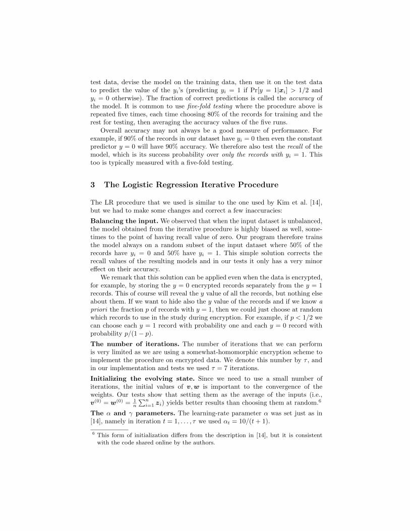
test data, devise the model on the training data, then use it on the test datato predict the value of the yi’s (predicting yi = 1 if Pr[y = 1|xi] > 1/2 andyi = 0 otherwise). The fraction of correct predictions is called the accuracy ofthe model. It is common to use five-fold testing where the procedure above isrepeated five times, each time choosing 80% of the records for training and therest for testing, then averaging the accuracy values of the five runs.

Overall accuracy may not always be a good measure of performance. Forexample, if 90% of the records in our dataset have yi = 0 then even the constantpredictor y = 0 will have 90% accuracy. We therefore also test the recall of themodel, which is its success probability over only the records with yi = 1. Thistoo is typically measured with a five-fold testing.

3 The Logistic Regression Iterative Procedure

The LR procedure that we used is similar to the one used by Kim et al. [14],but we had to make some changes and correct a few inaccuracies:

Balancing the input. We observed that when the input dataset is unbalanced,the model obtained from the iterative procedure is highly biased as well, some-times to the point of having recall value of zero. Our program therefore trainsthe model always on a random subset of the input dataset where 50% of therecords have yi = 0 and 50% have yi = 1. This simple solution corrects therecall values of the resulting models and in our tests it only has a very minoreffect on their accuracy.

We remark that this solution can be applied even when the data is encrypted,for example, by storing the y = 0 encrypted records separately from the y = 1records. This of course will reveal the y value of all the records, but nothing elseabout them. If we want to hide also the y value of the records and if we know apriori the fraction p of records with y = 1, then we could just choose at randomwhich records to use in the study during encryption. For example, if p < 1/2 wecan choose each y = 1 record with probability one and each y = 0 record withprobability p/(1− p).The number of iterations. The number of iterations that we can performis very limited as we are using a somewhat-homomorphic encryption scheme toimplement the procedure on encrypted data. We denote this number by τ , andin our implementation and tests we used τ = 7 iterations.

Initializing the evolving state. Since we need to use a small number ofiterations, the initial values of v,w is important to the convergence of theweights. Our tests show that setting them as the average of the inputs (i.e.,v(0) = w(0) = 1

n

∑ni=1 zi) yields better results than choosing them at random.6

The α and γ parameters. The learning-rate parameter α was set just as in[14], namely in iteration t = 1, . . . , τ we used αt = 10/(t+ 1).

6 This form of initialization differs from the description in [14], but it is consistentwith the code shared online by the authors.

For the moving average smoothing parameter γ, Kim et al. stated in [14]that they used γ ∈ [0, 1], but positive γ values result in bad performance of theNesterov algorithm. Instead, we used negative values for gamma as suggested in[5]: Setting λ0 = 0, we compute for t = 1, . . . , τ

λt =1 +

√1 + 4λ2t−1

2and γt =

1− λt−1λt

.

The values of γ for the first few steps are therefore γ ≈ (1, 0,−0.28,−0.43,−0.53,−0.6,−0.65, . . .)

Precision. We tested our procedure in order to decide how much precision isneeded since the CKKS scheme only offers limited precision. Our tests foundno significant difference in performance, even with only six bits of precision(i.e. error of upto 2−7 per operation). We therefore decided to set the precisionparameter for the homomorphic scheme at r = 8, corresponding to 2−8 error.As there was no real effect, we ran most of our plaintext tests below with fullprecision.

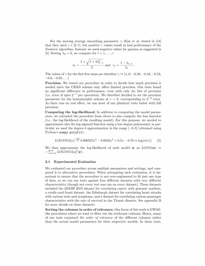
Computing the log-likelihood. In addition to computing the model param-eters, we extended the procedure from above to also compute the loss function(i.e., the log-likelihood of the resulting model). For this purpose, we needed toapproximate also the log-sigmoid function using a low-degree polynomial, in par-ticular we used the degree-4 approximation in the range [−8, 8] (obtained usingPython’s numpy.polyfit):

LOGSIG4(x)def= 0.000527x4 − 0.0822x2 + 0.5x− 0.78 ≈ log(σ(x)) (5)

We then approximate the log-likelihood of each model w as LOSS(w) ≈−∑n

i=1 LOGSIG4(zTi w).

3.1 Experimental Evaluation

We evaluated our procedure across multiple parameters and settings, and com-pared it to alternative procedures. When attempting such evaluation, it is im-portant to ensure that the procedure is not over-engineered to fit just one typeof data, so we run our tests against four different datasets with very differentcharacteristics (though not every test was run on every dataset). These datasetsincluded the iDASH 2018 dataset for correlating cancer with genomic markers,a credit-card fraud dataset, the Edinburgh dataset for correlating heart attackswith various tests and symptoms, and a dataset for correlating various passengercharacteristics with the rate of survival in the Titanic disaster. See appendix Bfor more details on these datasets.

Sorting the columns in order of relevance. One focus of this work is GWAS-like procedures where we want to filter out the irrelevant columns. Hence, manyof our tests examined the order of relevance of the different columns ratherthan the actual model parameters for their respective models. In these tests,

we computed all the LR models, one model per SNP (all models containingthe clinical variables), approximated the log-likelihood for each, and ordered theSNPs in decreasing order of their log-likelihood. This order is our procedure’sestimate of the order of relevance of the different SNPs to the condition. Wethen used the following methodology to evaluate the “quality” of this ordering:

– We applied the Matlab implementation of LR to re-compute the LR modelon the same data, using the glmfit function. The resulting LR models (oneper SNP) could be different than those produced by our iterative procedure;

– Next, we ran a five-fold test on the data using Matlab’s glmval to computethe predicted condition values, and computed the accuracy and recall foreach model;

– Finally, we plotted the accuracy and recall values against the order ofcolumns from our iterative procedure.

If the procedure works well, we expect a decreasing order of accuracy and recall,since the first models in the order are supposed to correspond to the most relevantSNPs, and hence to the highest accuracy and recall values.

We compared the column ordering from our iterative procedure to the or-dering generated by the p-values of the semi-parallel algorithm of Sikorska etal. [18]. (We used the R implementation provided by the iDASH organizers forthat purpose). We also tested the column ordering using the accuracy and re-call results as produced by the Matlab LR models (using glmfit and glmval),plotting them against the column ordering of the semi-parallel algorithm.

We stress that for both orderings, we plot the exact same accuracy andrecall numbers, i.e. the ones corresponding to the Matlab LR models. The onlydifference is the order in which we plot these numbers.

Evaluating the model parameters. Since our procedure yields not onlythe log-likelihood (a.k.a. p-value) for each model but also the model parame-ters themselves, we ran a few tests to examine how well these models perform.Namely, we compared the accuracy and recall of our models with those of theMatlab LR models on the same data. Again, we plotted all the accuracy andrecall results in the order of columns of our iterative procedure.

Different approximations of the sigmoid function. We tested our iterativeprocedure in two settings, one using nine iterations with the degree-3 approx-imation of the sigmoid, and the other using seven iterations with the degree-7approximation. While there were no significant differences in the order of SNPsproduced by the two variants, the model parameters produced by the degree-7approximation were often improved than those produced by the degree-3 approx-imation. We therefore ran most of our tests using only the seven-step degree-7approximation.

3.2 Accuracy and Recall Results

Here, we summarize the test results. All of these tests were run with our iterativeprocedure using the degree-7 approximation of the sigmoid function and τ = 7

iterations. All accuracy and recall results below were obtained using five-foldtesting (described in section 2.2). One point that needs care when running afive-fold test, is ensuring that the test data has similar characteristics to thetraining data: Some datasets are collected from multiple sources, hence the firstrecords may have very different characteristics than the last ones. (In particularthe data provided for the iDASH competition had that problem.) Randomizingthe order of the records in the dataset before running the test fixes this.

Comparing the column ordering, iterative vs. semi-parallel. As we ex-plained above, we run our iterative procedure and the semi-parallel algorithmfrom [18] side by side on the same data, computing the p-values from each andordering the SNPs according to these p-values. We then used the Matlab im-plementation of LR to compute the accuracy and recall values of the modelcorresponding to each SNP (with the same clinical variable), and plotted theseaccuracy and recall values in the two orders.

The results for the iDASH dataset are depicted in fig. 2. For that dataset, thetwo orders more or less coincide for the most relevant 1500 columns or so (out of10643). For the next 1500 columns, the orders are no longer the same. Moreover,while the accuracy results are very similar, the iterative ordering yields betterrecall values than the semi-parallel ordering. The last 8000 columns no longercontain much information on the condition variable, hence the ordering of thesecolumns is essentially random. We also ran the same test for the credit-card frauddataset, which contains only 30 columns. Here while the two orders identify thesame top nine, middle seven, and bottom fourteen columns, the ordering withineach of the first two groups was somewhat more accurate for the semi-parallelalgorithm than for the iterative method.

Comparing the iterative vs. Matlab models. Next, we tried to evaluatethe quality of the models generated by the iterative method to the standard LRmodels of Matlab. Since the iterative method with so few steps is only a crudeapproximation, we expected the Matlab model to perform better, but wanted tocheck by how much. We therefore computed for each column the accuracy andrecall values of both models (iterative vs. Matlab), and plotted them againstthe p-value ordering from our procedure. (See the full version for a plot of theresults.)

To our surprise, the crude approximated model computed by the iterativemethod performed at least as well (and sometimes better) than the LR modelthat Matlab computed for the same data. We can see that the iterative modelhas some bias for outputting y = 1, resulting in better recall and somewhatworse accuracy values. For example, notice that around the 1000’th SNP theiterative model has recall value of 1, while the Matlab model’s recall values arecapped around 0.9 (with essentially the same accuracy). We ran the same testalso on the Titanic dataset, and again the iterative models did about as well(and sometimes better) than the Matlab models.

The Edinburgh dataset. We also ran our iterative procedure on the Edinburghdatasets computing the accuracy/recall for the Matlab model for each column

and plotting these values against the p-value ordering of the columns as producedby the iterative procedure.

3.3 Conclusions and Some Comments

Summarizing the tests above, the iterative procedure that we used produces mod-els which are competitive to what we get from Matlab, and that the relevanceorder that we get from our p-values is just as reasonable as the one obtainedby the semi-parallel algorithm. While the semi-parallel algorithm is faster (es-pecially when there are many covariates), for a small number of covariates theiterative procedure has reasonable performance. A reasonable conclusion to drawis that one should still run the semi-parallel algorithm in the context of GWAS,but use the iterative model if it is desired to also get the actual LR models (inaddition to ordering the columns by relevance).

In this context, the semi-parallel algorithm assumes that the model weightsfor the covariates are more or less the same when you devise a model for justthe covariates as when you devise a model for the covariates and a single SNP.For the iDASH dataset, this was true for most SNPs (since most SNPs werenot correlated with the condition at all), but our tests showed that it seems tonot be true for the most relevant SNPs. This observation implies that while thesemi-parallel algorithm is a good screening tool to filter out the irrelevant SNPs(for which the assumption on the covariates should hold), it probably should notbe used to compute the model parameters for the more relevant SNPs.

Finally, during our work we encountered two minor bugs/inconsistencies inthe literature, notified the relevant authors, and document them in appendix A.

4 Homomorphic Evaluation of the LR Procedure

To evaluate the procedure from section 3 on encrypted data, we used the CKKSapproximate-number HE scheme of Cheon et al. [7], which we implemented inthe HElib library [10]. The underlying plaintext space of this scheme are complexnumbers (with limited precision), and the scheme can pack many such complexnumbers in a single ciphertext. In section 4.3 below, we briefly describe somedetails of our HElib-based implementation, see the original work [7] for detailsabout the scheme itself. The API provided by our implementation is as follows:

Parameters. Security parameter λ, plus two functionality parameters: Thepacking parameter ` determines how many complex numbers can be encodedin a single ciphertext, and the accuracy parameter r determines the supportedprecision. Operations of the scheme are accurate up to additive noise of magni-tude bounded by 2−r. We refer to entries in the encrypted vectors as plaintextslots.

Noisy Encoding. The native objects manipulated in the CKKS scheme belongto an algebraic ring (specifically algebraic integers in cyclotomic number fields).The scheme provides routines to encode and decode plaintext complex vector

v ∈ C` into and out of that ring. However the encoding is noisy, which introducesadditive errors of magnitude up to 2−r in each entry.

Encryption, decryption, and homomorphic operations. Once encoded inthe “native ring,” data can be encrypted and decrypted using the public andsecret keys, respectively.

– The scheme supports addition and multiplication operations, both plaintext-to-ciphertext and ciphertext-to-ciphertext, including element-wise addi-tion/multiplication on the underlying complex vectors. Providing wt =ut + vt for every entry t for addition, and similarly wt = ut · vt for mul-tiplication.

– There are procedures (which are essentially free) for multiplying and dividingciphertexts by real numbers, namely setting vt = ut ·x or vt = ut/x for all t.

– Included is the support for “homomorphic automorphisms”. Our applicationuses automorphisms for computing complex conjugates. Namely, given anencoded (or encrypted) vector u, the conjugate operation outputs a similarlyencoded/encrypted vector v such that vt = ut for every entry t. Used tohomomorphically extract the real and imaginary parts, via im(x) = (x−x)/2iand re(x) = (x+ x)/2 (with i denoting the imaginary square root of −1).

All the operations above (including encoding and encryption) accrue additiveerrors. Namely, an operation can return a vector v′ that differs from the intendedresult v, with the guarantee that for every entry t we have |vt − v′t| ≤ 2−r.

4.1 The Homomorphic LR Procedure

The input to the LR procedure consists of n records, each containing k covariates(i.e., clinical variables such as age or gender), N genomic markers (or SNPs),and a single binary condition variable (sick or healthy). Our solution is tailoredfor the case where k is small (up to five), N is large (many thousands) and thenumber of records is moderate (hundreds to a few thousands).

Our goal is to compute N (approximate) LR models, one per SNP, where thet’th model includes parameters for all the k clinical variables and the (single)t’th SNP. As described in section 3, our approach follows the approach by Kimet al. [14]. Namely, we run an iterative method using Nesterov’s algorithm anda low-degree approximation of the sigmoid function implemented on top of theCKKS approximate-number homomorphic encryption scheme [7].

The main difference is that we use the inherent SIMD properties of CKKSto compute all the N models at once: We run the LR computation in a bitslicemode, where we pack the data into a number of N -vectors with the t’th entryin each vector corresponds to the t’th model. Each input record has k+ 2 inputciphertexts: One for the condition variable (with all the slots holding the samecondition bit), one for each of the covariates (with all the slots holding the samecovariate value), and one more ciphertext for all the SNPs (with the differentSNPs in the different slots).

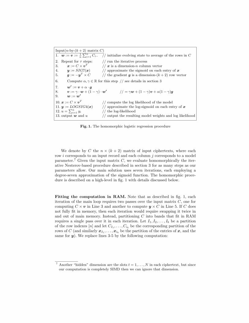
Input(n-by-(k + 2) matrix C)

1. w := v := 1n

∑ni=1 Ci− // initialize evolving state to average of the rows in C

2. Repeat for τ steps: // run the iterative process3. x := C × vT // x is a dimension-n column vector4. y := SIG7(x) // approximate the sigmoid on each entry of x5. g := −yT × C // the gradient g is a dimension-(k + 2) row vector

6. Compute α, γ ∈ R for this step // see details in section 3

7. w′ := v + α · g8. v := γ ·w + (1− γ) ·w′ // = γw + (1− γ)v + α(1− γ)g9. w := w′

10. x := C × vT // compute the log likelihood of the model11. y := LOGSIG4(x) // approximate the log-sigmoid on each entry of x12. u =

∑ni=1 yi // the log-likelihood

13. output w and u // output the resulting model weights and log likelihood

Fig. 1. The homomorphic logistic regression procedure

We denote by C the n × (k + 2) matrix of input ciphertexts, where eachrow i corresponds to an input record and each column j corresponds to a modelparameter.7 Given the input matrix C, we evaluate homomorphically the iter-ative Nesterov-based procedure described in section 3 for as many steps as ourparameters allow. Our main solution uses seven iterations, each employing adegree-seven approximation of the sigmoid function. The homomorphic proce-dure is described on a high-level in fig. 1 with details discussed below.

Fitting the computation in RAM. Note that as described in fig. 1, eachiteration of the main loop requires two passes over the input matrix C, one forcomputing C × v in Line 3 and another to compute y × C in Line 5. If C doesnot fully fit in memory, then each iteration would require swapping it twice inand out of main memory. Instead, partitioning C into bands that fit in RAMrequires a single pass over it in each iteration. Let I1, I2, . . . , Ib be a partitionof the row indexes [n] and let CI1 , . . . , Cib be the corresponding partition of therows of C (and similarly xI1 , . . . ,xib be the partition of the entries of x, and thesame for y). We replace lines 3-5 by the following computation:

7 Another “hidden” dimension are the slots t = 1, . . . , N in each ciphertext, but sinceour computation is completely SIMD then we can ignore that dimension.

[...]2. Repeat for τ steps: // run the iterative process2a. g := 02. For h = 1 to b // go over the bands of C3′. x

Ih:= CIh × vT // xIh is part of x

4′. yIh

:= SIG7(xIh

) // approximate the sigmoid on each entry of x

5′. g := g − yTIh× CIh // the contribution of CIh to the gradient

6. [...] // continue with the update of v,w as before

Computing the log likelihood. As we explained in section 2.2, after comput-ing the model parameters w we need to also evaluate this model by computingits p-value, i.e, the loss function from eq. (1). This computation is very similarto the computation of the gradient, but here we use the approximation of thelog-sigmoid LOGSIG4 instead of the SIG7 approximation of the sigmoid itself.Namely we first compute x := C ×w, then y := LOGSIG4(x), and finally sumup (or average) the entries in the vector y.

4.2 Fewer Multiplications Via Complex Packing

We implemented a second variant of our solution, which is faster and uses halfthe number of ciphertexts, but adds more noise per iteration. This was done bypacking the data more tightly, utilizing both the real part and the imaginary partof each plaintext slot, thus encrypting two input records in each ciphertext (onein the real part of all the slots and the other in the imaginary parts). Specifically,let z2i−1,j , z2i,j be the two real values that were encrypted in the two ciphertextsC2i−1,j , C2i,j in the matrix C from above. In the new variant we instead use asingle ciphertext C ′i,j , encrypting the complex value z′i,j = z2i−1,j + i · z2i,j (withi the imaginary square root of −1). Let C ′ = [C ′i,j ] be the resulting ciphertextmatrix, and N ′ = dN/2e be the number of rows in the matrix C ′.

During the computation we maintain the evolving state vectors v,w as realvectors (i.e., their imaginary part is zero). This sometimes requires spliting theencrypted complex numbers into their real and imaginary parts (using the con-jugate operation mentioned above). For example, we initialize the evolving stateby computing the average of the (complex) rows of C ′. Then we split the resultinto its real and complex parts and average the two.

Similarly, we sometimes also need to assemble two real values into a complexone, just by computing zc = zr + i ·zi homomorphically. These split and assembleoperations cause this variant to accrue more noise than before. However, it useshalf as many input ciphertexts and roughly half as many operations per iterationof the Nesterov algorithm.

Computing the gradient. The most interesting aspect of this complex-packedprocedure is the computation of the gradient in Steps 3-5 from fig. 1. The mul-tiplication in Step 3 is quite straightforward: since v encrypts a real vector, we

can compute x′ := C ′ × vT just as before and the multiplication by v operatesseparately on the real and imaginary parts of C ′.

To apply the sigmoid function, requires spliting the resulting x′ into itsreal and imaginary components and compute the sigmoid approximation oneach of them separately. Namely, we set xr := re(x) and xi := im(x), thenyr := SIG7(xr) and yi := SIG7(xi). To save on noise, we fold into the sigmoidcomputation some of the multiply-by-constant operations from splitting x′.

More interesting is how to compute the product y × C ′ from Step 5 withour tightly packed version of the ciphertext matrix. Here we use the happycoincidence that for complex numbers we have (a + ib)(a′ − ib′) = aa′ + bb′ +i · something, giving us the inner product 〈(a, b), (a′, b′)〉 in the real part. Wetherefore pack y′ := yr − i · yi, compute g′ = −y × C ′, and the real part of g′

turns out to be exactly the gradient vector that we need. To see this, recall thatfor all i, j we have y′j = y2j−1 − i · y2j and C ′i,j = z2j−1 + i · z2j , and therefore

g′j =

N ′∑i=1

y′i · C ′i,j =

N/2∑i=1

(y2i−1 − i · y2i

)·(z2i−1,j + i · z2i,j

)=

N/2∑i=1

(y2i−1 · z2i−1,j + y2i · z2i,j + i · something

)=( N∑i=1

yi · zi,j)

+ i · something′.

We complete the gradient computation just by extracting the real part, g :=re(g′). This new gradient calculation performs half as many multiplications inthe inner-product steps (3 and 5), the same number of operations in the sigmoidstep 4, and a few more operations to split and recombine complex vectors fromreal and imaginary parts. Since the inner product operations are by far the mostexpensive parts of each Nesterov computation, this saves nearly half of the overallnumber of multiplications. However, in our tests it only saved about 20% of therunning time. (We think that this discrepancy is partially because we workedharder on optimized the standard procedure than the complex packed one.)

4.3 Implementing CKKS in HElib

The CKKS scheme from [7] is a Regev-type cryptosystem, with a decryptioninvariant of the form [〈sk, ct〉]q = pt, where sk, ct are the secret-key and ciphertextvectors, respectively, [·]q denotes reduction modulo q into the interval [−q/2, q/2],and pt is an element that encodes the plaintext and includes also some noise.

The CKKS scheme is similar in many ways to the BGV scheme from [4]:both schemes use an element pt of low norm, |pt| � q, and the homomorphicoperations are implemented almost exactly the same in both. The differencebetween these schemes lies in the way they interpret the element pt, i.e., how itis decoded into plaintext pt and noise e: We tend to think in the BGV of thelow-order bits of pt as pt and the high-order bits as e, and in CKKS it is theother way around. Specifically, the BGV decodes pt = pt + p · e, where p is theplaintext space modulus and |pt| < p, whereas CKKS decodes pt = e + ∆ · ptwhere ∆ is some scaling factor and (hopefully) |e| < ∆.

This difference in interpretation of pt implies very different plaintext algebrasfor the two schemes: While BGV deals with integral plaintext elements modulo p,in CKKS the plaintext elements are complex numbers with limited precision.Some other (rather small) differences between the homomorphic operations inBGV and CKKS are related to the way the scaling factor ∆ is handled:

– The plaintext modulus p in BGV typically does not change throughout thecomputation, but the scaling factor ∆ in CKKS does vary: Specifically, ∆ issquared on multiplication and is scaled via modulus switching.

– In both CKKS and BGV, ciphertexts can only be added when they aredefined relative to the same modulus q. However, it is also important forCKKS addition that they have the same scaling factor ∆.

Our CKKS implementation in HElib relies on the same chassis as the BGVcryptosystem that supports the required homomorphic operations and handlesany cyclotomic field.8 Differently from the way it is described in [7], the HElibimplementation does not rely on the application to use explicit scaling, insteadthe library can automatically scale all the ciphertexts as needed. Each ciphertextin our implementation is tagged with both a noise estimate and the scalingfactor ∆ and the library uses these tags to decide how and when to scale theseciphertexts using modulus-switching. These scaling decisions balance the needto scale the ciphertexts down before multiplication to keep the noise small withthe need to keep the scaling factor ∆ sufficiently larger than the noise element e.

The cryptosystem is initialized with an accuracy parameter r that from theapplication perspective roughly means the additive noise terms in the variousoperations is bounded by 2−r in magnitude. The library tries to ensure that op-erations with added noise term η will only be applied to ciphertexts with scalingfactors ∆ ≥ η · 2r. Note, that this logic only “does the right thing” when thecomplex values throughout the computation are close to one in magnitude. Forsmaller values, the requested accuracy bound will typically not be enough, whilefor larger values the implementation will spend too much resources trying tokeep the precision way too high. The logic works quite well for the LR proce-dure (section 3) where indeed all the encrypted quantities are kept at size Θ(1).

4.4 Performance of the Homomorphic Procedure

We tested the running time and memory consumption in a few different settings,depending on the number of available threads, and the number of bands in thematrix C. (As we explained in section 4.1, using more bands is useful when themachine has limited RAM and cannot fit all the encrypted input ciphertextsin memory at once.) We also tested the complex packing optimization fromsection 4.2 vs. the “standard” way of packing only real numbers in the slots.

These tests were run on a machine with Intel E5-2640 CPU running at2.5GHz, with 2×12 cores, 64 GB memory (split 32GB for each chip in aNUMA configuration), and 15MB cache. The software configurations (on Ubuntu

8 Our logistic regression procedure uses a power of two cyclotomic field for efficiency.

16.04.5) included HElib commit dbaa108b66c5 from Sep 2018, NTL version11.3.2, GMP version 6.1.2, and Armadillo version 9.200.7. All compiled with gcc8.1.0 including our LR code.

Parameters. The parameters were chosen so as to get at least 128 security levelwhile having enough levels to complete seven iterations (followed by computingthe log likelihood of the resulting model). Specifically, the largest modulus inthe chain had |q| = 900 bits, and the scheme was instantiated over the m’thcyclotomic field with m = 217 = 131072 (so the dimension of the relevant latticewas φ(m) = 65536). This setting gave us estimated security level of 142 bits.These parameters give us φ(m)/2 = 32768 slots in which to pack data, so wecould compute up to 32768 LR models in parallel.

The results that we describe below were measured on the iDASH 2018dataset, where each model has three clinical variables and a single SNP. Thisdataset had only 10643 SNPs, so we only packed that many numbers in the slots,but the performance numbers are not affected by the number of “empty slots,”we would have identical results even if all 32767 slots were filled.

On the other hand, the number of records in the training set does influencethe running time (as well as the memory consumption). Here we used the factthat small LR models can be computed accurately by sub-sampling the data.The common “one in ten” rule of thumb states that a model with k featuresrequires at least 10k records with 0 and 10k records with 1. Since in these testswe had four features in each model (three clinical variables and one SNP), andsince we sub-sampled the data to get 50% 0’s and 50% 1’s, then we needed atleast 80 total record, and we run all our tests on 100 records in the training test.

Without the complex-packing optimization, each iteration of the Nesterovprocedure took four levels in the modulus chain. This is a little surprising, aseach iteration includes a degree-7 polynomial sandwiched between two vector-matrix multiplications so we expect it to take five levels rather than four. Thereason is that we used 44 bits “wide” levels, and the noise management logicof HElib performed two consecutive operations at the same level. This indicatessome waste in the HElib noise management. With complex packing, we couldonly perform six iterations with the same parameters as each iteration of theNesterov procedure used an average six levels.

Results. The results are described in Tables 1 and 2. The optimization of usingcomplex packing cuts the input-reading time in half (as there are half as manyciphertexts), but only reduces the running time by about 20% (for the samenumber of iterations). There is approximately a linear speedup when the numberof threads is increased from one to twelve, but not more due to cache contentionon the testing server architecture. The memory requirements grow slowly withthe number of threads, twelve threads consumed 1.5× to 2× more memory thana single threads.

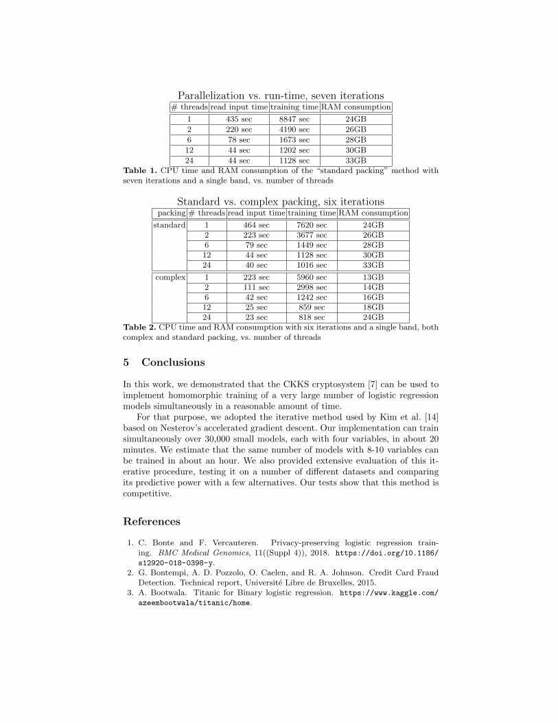
Parallelization vs. run-time, seven iterations# threads read input time training time RAM consumption

1 435 sec 8847 sec 24GB

2 220 sec 4190 sec 26GB

6 78 sec 1673 sec 28GB

12 44 sec 1202 sec 30GB

24 44 sec 1128 sec 33GBTable 1. CPU time and RAM consumption of the “standard packing” method withseven iterations and a single band, vs. number of threads

Standard vs. complex packing, six iterationspacking # threads read input time training time RAM consumption

standard 1 464 sec 7620 sec 24GB2 223 sec 3677 sec 26GB6 79 sec 1449 sec 28GB12 44 sec 1128 sec 30GB24 40 sec 1016 sec 33GB

complex 1 223 sec 5960 sec 13GB2 111 sec 2998 sec 14GB6 42 sec 1242 sec 16GB12 25 sec 859 sec 18GB24 23 sec 818 sec 24GB

Table 2. CPU time and RAM consumption with six iterations and a single band, bothcomplex and standard packing, vs. number of threads

5 Conclusions

In this work, we demonstrated that the CKKS cryptosystem [7] can be used toimplement homomorphic training of a very large number of logistic regressionmodels simultaneously in a reasonable amount of time.

For that purpose, we adopted the iterative method used by Kim et al. [14]based on Nesterov’s accelerated gradient descent. Our implementation can trainsimultaneously over 30,000 small models, each with four variables, in about 20minutes. We estimate that the same number of models with 8-10 variables canbe trained in about an hour. We also provided extensive evaluation of this it-erative procedure, testing it on a number of different datasets and comparingits predictive power with a few alternatives. Our tests show that this method iscompetitive.

References

1. C. Bonte and F. Vercauteren. Privacy-preserving logistic regression train-ing. BMC Medical Genomics, 11((Suppl 4)), 2018. https://doi.org/10.1186/

s12920-018-0398-y.2. G. Bontempi, A. D. Pozzolo, O. Caelen, and R. A. Johnson. Credit Card Fraud

Detection. Technical report, Universite Libre de Bruxelles, 2015.3. A. Bootwala. Titanic for Binary logistic regression. https://www.kaggle.com/

azeembootwala/titanic/home.

4. Z. Brakerski, C. Gentry, and V. Vaikuntanathan. Fully homomorphic encryp-tion without bootstrapping. In Innovations in Theoretical Computer Science(ITCS’12), 2012. Available at http://eprint.iacr.org/2011/277.

5. S. Bubeck. ORF523: Nesterov’s accelerated gradient descent. https://blogs.

princeton.edu/imabandit/2013/04/01/acceleratedgradientdescent, accessedJanuary 2019, 2013.

6. H. Chen, R. Gilad-Bachrach, K. Han, Z. Huang, A. Jalali, K. Laine, andK. Lauter. Logistic regression over encrypted data from fully homomorphic en-cryption. BMC Medical Genomics, 11((Suppl 4)), 2018. https://doi.org/10.

1186/s12920-018-0397-z.7. J. H. Cheon, A. Kim, M. Kim, and Y. S. Song. Homomorphic encryption for

arithmetic of approximate numbers. In ASIACRYPT (1), volume 10624 of LectureNotes in Computer Science, pages 409–437. Springer, 2017.

8. J. L. H. Crawford, C. Gentry, S. Halevi, D. Platt, and V. Shoup. Doing realwork with FHE: the case of logistic regression. In M. Brenner and K. Rohloff,editors, Proceedings of the 6th Workshop on Encrypted Computing & Applied Ho-momorphic Cryptography, WAHC@CCS 2018, pages 1–12. ACM, 2018. https:

//eprint.iacr.org/2018/202.9. C. Gentry. Fully homomorphic encryption using ideal lattices. In Proceedings of

the 41st ACM Symposium on Theory of Computing – STOC 2009, pages 169–178.ACM, 2009.

10. S. Halevi and V. Shoup. HElib - An Implementation of homomorphic encryption.https://github.com/shaih/HElib/, Accessed January 2019.

11. K. Han, S. Hong, J. H. Cheon, and D. Park. Efficient logistic regression on largeencrypted data. Cryptology ePrint Archive, Report 2018/662, 2018. https://

eprint.iacr.org/2018/662.12. Integrating Data for Analysis, Anonymization and SHaring (iDASH). https://

idash.ucsd.edu/.13. R. L. Kennedy, H. S. Fraser, L. N. McStay, and R. F. Harrison. Early diag-

nosis of acute myocardial infarction using clinical and electrocardiographic dataat presentation: derivation and evaluation of logistic regression models. Euro-pean Heart Journal, 17(8):1181–1191, Aug. 1996. Data obtained from https:

//github.com/kimandrik/IDASH2017/tree/master/IDASH2017/data/edin.txt.14. A. Kim, Y. Song, M. Kim, K. Lee, and J. H. Cheon. Logistic regression model train-

ing based on the approximate homomorphic encryption. BMC Medical Genomics,11(4):83, Oct 2018.

15. M. Kim, Y. Song, S. Wang, Y. Xia, and X. Jiang. Secure logistic regression basedon homomorphic encryption: Design and evaluation. JMIR Med. Inform., 6(2):e19,2018. DOI: 10.2196/medinform.8805. Also available from https://eprint.iacr.

org/2018/074.16. Y. Nesterov. Introductory Lectures on Convex Optimization: A Basic Course,

volume 87 of Applied Optimization. Springer US, 2004. https://doi.org/10.

1007/978-1-4419-8853-9.17. A. D. Pozzolo, O. Caelen, R. A. Johnson, and G. Bontempi. Calibrating Probabil-

ity with Undersampling for Unbalanced Classification. In 2015 IEEE SymposiumSeries on Computational Intelligence, pages 159–166, Dec. 2015.

18. K. Sikorska, E. Lesaffre, P. J. Groenen, and P. H. Eilers. GWAS on your notebook:fast semi-parallel linear and logistic regression for genome-wide association studies.BMC Bioinformatics, 14:166, 2013.

19. Logistic regression. https://en.wikipedia.org/wiki/Logistic_regression#

Discussion. Accessed January 2017.

A Corrections in the Literature

During our work we encountered two minor bugs/inconsistencies in the litera-ture. We have notified the relevant authors and document these issues here:

– The Matlab code used in the iDASH 2017 competition had a bug in theway it computed the recall values, computing it as false positive+true positive

false negative+true positive

instead of true positivefalse negative+true positive .

– Some of the mean-squared-error (MSE) results reported in [14] seem incon-sistent with their accuracy values: For the Edinburgh dataset, they reportaccuracy value of 86%, but MSE of only 0.00075. We note that 86% accuracyimplies MSE of at least 0.14 · (0.5)2 = 0.035 (likely a typo).

B The Datasets that We Used

Recall that we tested the iterative procedure against a few different datasets, toensure that it is not “tailored” too much to the characteristics of just one typeof data. We had some difficulties finding public datasets that we could use forthis evaluation, eventually we converged on the following four:

– The iDASH 2018 dataset, as provided by the organizers of the competition,is meant to correlate various genetic markers with the risk of developingcancer. It consists of 245 records, each with a binary condition (cancer ornot), three covariates (age, weight, and height), and 10643 markers (SNPs).The last 120 records were missing the covariates, so we ran our procedureby replacing each missing covariate by the average of the same covariate inthe other records.

– A credit card dataset [2] attempts to correlate credit-card fraud with ob-served characteristics of the transaction. This dataset has 984 records eachwith thirty columns.

– The Edinburgh dataset [13] correlates the condition of Myocardial Infarc-tion (heart attack) in patients who presented to the emergency room in theEdinburgh Royal Infirmary in Scotland with various symptoms and test re-sults (e.g., ST elevation, New Q waves, Hypoperfusion, depression, vomiting,etc.). The same dataset was also used to evaluate the procedure of Kim etal. [14]. The data includes 1253 records, each with nine features.

– The Titanic dataset [3], consisting of 892 records with sixteen features, cor-relating passenger’s survival in that disaster with various characteristics suchas gender, age, fare, etc.

The first dataset comes with a distinction between SNPs and clinical vari-ables, but the other three have just the condition variable and all the rest. Wehad to decide which of the features (if any) to use for covariates. We note thatwhatever feature we designate as covariate will be present in all the models, sochoosing a feature with very high signal will make the predictive power of allthe models very similar. We therefore typically opted to choose for a covariatethe features which is least correlated with the condition. We also ran the sametest with no covariates, and the results were very similar.

C Model Evaluation Figures

iDASH data column ordering: iterative vs. semi-parallel

(a) Accuracy, iterative Order (b) Recall, iterative Order

(c) Accuracy, semi-parallel order (d) Recall, semi-parallel order

Fig. 2. Accuracy/recall of the Matlab LR models for the iDASH 2018 dataset orderedaccording to the p-value order of the iterative procedure (top) or the semi-parallelalgorithm (bottom).