Homology Theory

JWR

Feb 6, 2005

1 Abelian Groups

1.1. Let {Gα}α∈Λ be an indexed family of Abelian groups. The direct product∏α∈Λ Gα of this family is the set of all functions g defined on the index set Λ

such that g(α) ∈ Gα for α ∈ Λ; the direct sum is the subgroup⊕

α∈Λ

Gα ⊂∏

α∈Λ

Gα

of those g of finite support, i.e. g(α) = 0 for all but finitely many α. A freeAbelian group is a group which is isomorphic to G =

⊕α∈Λ Z for some index

set Λ. The elements eα ∈⊕

α∈Λ Gα defined by eα(α) = 1 and αα(β) = 0 forβ 6= α have the property that every element g ∈ G is uniquely expressible as afinite sum

g =∑α

nαeα

where the coefficients nα are integers; such a system of elements of a free Abeliangroup is call a free basis. It is easy to see that the cardinality a free basis isindependent of the choice of the basis; it is called the rank of the free group.An Abelian group G is said to be finitely generated iff there is a surjectivehomomorphism h : Zn → G.

1.2. A graded Abelian group is an Abelian group C equipped with a witha direct sum decomposition

C =⊕

n∈ZCn.

Unless otherwise specified we assume the grading is nonnegative meaning thatCn = 0 for n < 0. A subgroup A of C is called graded iff

A =⊕

n∈ZAn where An := A ∩ Cn.

It is easy to see that the quotient is then also graded, i.e.

C/A =⊕

n∈Z(Cn/An).

1

The usage of the direct sum is a notational convenience only; it is better tothink of a graded Abelian group as a sequence {Cn}n of Abelian groups.

1.3. homomorphism h : A → B between graded Abelian groups is said to shiftthe grading by r iff h(An) ⊂ Bn+r for all n; h is said to preserve the gradingiff it shifts the grading by 0. The kernel, image, and hence also cokernel of h isgraded. The graded Abelian groups and grade shifting homomorphisms form acategory as do the graded Abelian groups and grade preserving homomorphisms,

1.4. Suppose that α : A → B and β : B → C are homomorphisms of Abeliangroups. We say that the sequence

Aα // B

β // C

is exact at B iff the kernel of β is the image of α, i.e. α(A) = β−1(0). Asequence

· · · // Cn+1// Cn

// Cn−1// · · ·

is called exact iff it is exact at each Cn. When the sequence terminates (at eitherend), no condition is placed on the group at the end. To impose a condition anextra zero is added. Thus a short exact sequence is an exact sequence

0 // Aα // B

β // C // 0,

i.e. it is exact at A, B, and C. For a short exact sequence the map α is injective,the map β is surjective, and C is isomorphic to the quotient B/α(A). Often Ais a subgroup of B and α is the inclusion so C ≈ B/A. More generally, an exactsequence

0 // K // Aα // B,

gives an isomorphism from K to the kernel α−1(0) of α, and an exact sequence

Aα // B // C // 0,

gives an isomorphism from C to the cokernel B/α(A) of α.

Exercise 1.5. Show that for a short exact sequence as in 1.4 the following areequivalent:

(1) There is an isomorphism φ : A⊕ C → B with φ|A = α and β ◦ φ|C = idC .

(2) There is a homomorphism λ : B → A with λ ◦ α = idA.

(3) There is a homomorphism ρ : C → B with β ◦ ρ = idC .

When these three equivalent conditions hold we say that the exact sequencesplits or that the subgroup α(A) ⊂ B splits in B.

2

Exercise 1.6. Show that a short exact sequence as in 1.4 always splits whenC is free but give an example of a short exact sequence which doesn’t split eventhough A and B are free.

Exercise 1.7. The concepts of 1.4 remain meaningful for non Abelian groupsalthough it is customary to use multiplicative notation (1, ab, A × B) ratherthan additive notation (0, a+b, A⊕B). Show that the implications (1) ⇐⇒ (2)and (1) =⇒ (3) remain true in the non Abelian case but give an example where(3) =⇒ (1) fails.

Lemma 1.8 (Smith Normal Form). For any integer matrix A ∈ Zm×n thereare square integer matrices P ∈ Zm×m and Q ∈ Zn×n of determinant ±1 (soP−1 and Q−1 are integer matrices by Cramer’s rule) such that

PAQ−1 =[

D 0r×(n−r)

0(m−r)×r 0(m−r)×(n−r)

]

where D is a diagonal integer matrix of form

D =

d1 0. . .

0 dr

,

di > 0, and di divides di+1.

Proof. Use row and column operations to transform to a matrix where the leastcommon denominator of the entries is in the (1, 1) position and then use row andcolumn operations to transform so that the other entries in the first row and thefirst column to vanish. Then use induction on the remaining (m− 1)× (n− 1)matrix. As in elementary linear algebra, the row operations give P and thecolumn operations give Q. See Theorem 11.3 Page 55 of [7] for more details.

Corollary 1.9. A subgroup of a free Abelian group is free Abelian of lower orequal rank.

Proof. It follows from Smith Normal Form that the range of A is a free subgroup.It is easy to see that any subgroup of Zm is the range of A for some integermatrix A. Hence Smith Normal Form implies that See Lemma 11.1 page 53of [7] for a more direct argument. Lemma 11.2 page 54 of [7] shows that asubgroup of a free Abelian group is free Abelian even without the hypothesisthat the ambient group is finitely generated.

1.10. The torsion subgroup T (G) of an Abelian group G is the subgroup ofelements of finite order. It is not hard to see that if G is finitely generated thequotient G/T (G) is free and hence splits by Exercise 1.6. Lemma 1.8 yields thefollowing stronger

3

Corollary 1.11 (Fundamental Theorem of Abelian Groups). Let Afinitely generated Abelian group G has a direct sum decomposition

G = F ⊕ T (G), T (G) = Z/d1 ⊕ · · ·Z/dr

where F is free, di > 0, and di divides di+1.

Remark 1.12. The rank of the free group G/T (G) is also called the rank of Gitself. The tensor product Q⊗G of G with the rational numbers Q is a vectorspace over Q. It is easy to see that the dimension of the vector space Q⊗G isthe rank of G.

Exercise 1.13. The torus T 2 may be viewed as the quotient R2/Z2 of thegroup R2 by the subgroup Z2. Consider the linear map R2 → R2 and its inverserepresented by the matrices

A =[

3 54 7

], A−1 =

[7 −5

−4 3

].

As A has integer entries it defines a map f : T 2 → T 2 by

f(x + Z2) = Ax + Z2

for x ∈ R2. As A−1 also has integer entries, this map is a homeomorphism.How many fixed points does it have? (A fixed point of f is a point p ∈ T 2 suchthat f(p) = p.)

Lemma 1.14 (Five Lemma). Consider a commutative diagram

Ai //

α

²²

Bj //

β

²²

Cj //

γ

²²

Dk //

δ

²²

E

ε

²²A′

i′ // B′ j′ // C ′k′ // D′ `′ // E′

of Abelian groups and homomorphisms. Assume that the rows are exact andthat α, β, δ, and ε are isomorphisms. Then γ is an isomorphism.

2 Abstract Homology

2.1. A chain complex is a pair (C, ∂) consisting of a

C =⊕

n∈ZCn,

and a homomorphism ∂ : C → C called the boundary operator such that∂(Cn+1) ⊂ Cn and ∂2 = 0. The chain complex (C, ∂) will be denoted simplyby C when no confusion can result. If there are several chain complexes in thediscussion we write ∂C for ∂. A chain map from a chain complex (A, ∂A) to

4

a chain complex (B, ∂B) is a group homomorphism φ : A → B which preservesthe grading and satisfies

∂B ◦ φ = φ ◦ ∂A.

Chain complexes and chain maps form a category, i.e. the identity idC : C → Cis a chain map and the composition of chain maps is a chain map.

Remark 2.2. Unless otherwise specified we assume that chain complexes arenonnegative meaning that Cn = 0 for n < 0.

2.3. Let (C, ∂) be a chain complex, Z(C) = ∂−1(0) denote the kernel of ∂, andB(C) = ∂(C) denote the image of ∂. As ∂ shifts the grading by −1 these aregraded subgroups, i.e. B(C) =

⊕n Bn(C) and Z(C) =

⊕n Zn(C) where

Bn(C) := ∂(Cn+1) = B(C) ∩ Cn and Zn(C) := Z(C) ∩ Cn.

The condition ∂2 = 0 is equivalent to the condition B(C) ⊂ Z(C). The quotientH(C) := Z(C)/B(C) is called the homology group of C. This is also graded,namely H(C) =

⊕n Hn(C) where

Hn(C) := Zn(C)/Bn(C).

By Remark 2.2 Z0(C) = C0. An elements of B(C) is called a boundary, anelement of Z(C) is called a cycle, and an element of H(C) is called a homologyclass. A chain map φ : A → B sends boundaries to boundaries and cycles tocycles and hence induces a graded homomorphism

φ∗ : Hn(A) → Hn(B)

for each n. The operation which sends the chain complex C to the gradedgroup H(C) and sends the chain map φ : A → B to the graded homomorphismφ∗ : H(A) → H(B) is a functor, i.e.

(idC

)∗ = idH(C) and (ψ ◦ φ)∗ = ψ∗ ◦ φ∗.

Remark 2.4. A chain complex

· · · ∂ // Cn+1∂ // Cn

∂ // Cn−1∂ // · · ·

is exact at Cn (where n > 0) if and only if Hn(C) = 0. A chain complex whosehomology vanishes is sometimes called acyclic.

2.5. An augmented chain complex is a nonnegative chain complex C whichis equipped with an augmentation, i.e. a surjective homomorphism ε : C0 →Z such that ε ◦ ∂|C1 = 0. We use the augmentation to produce a modifiednonnegative chain complex C defined by

Cn = Cn for n > 0 and C0 = ε−1(0).

For an augmented chain complex, the reduced homology group H(C) is thehomology of the modified complex, i.e.

Hn(C) := Zn(C)/Bn(C)

5

where Zn(C) := Zn(C) for n > 0, Z0(C) := ε−1(0), and Bn(C) := Bn(C) forn ≥ 0. Obviously Hn(C) = Hn(C) for n > 0. A chain map φ : A → B betweentwo augmented chain complexes is said to be augmentation preserving iffεB ◦ (φ|A0) = εA. Just as for chain maps, an augmentation preserving chainmap induces a graded homomorphism

φ∗ : H(A) → H(B)

on reduced homology.

Remark 2.6. An exact sequence 0 → A → B → C → 0 of augmented chaincomplexes gives rise to an exact sequence 0 → A → B → C → 0 of themodified chain complexes. An augmented chain complex can be viewed aschain complex with C−1 = Z and ∂|C0 = ε. This construction gives a chaincomplex with the same homology as C but is inconvenient because it does notpreserves exact sequence of chain complexes in the aforementioned sense: asequence 0 → Z→ Z→ Z→ 0 is never exact.

2.7. Consider short exact sequence

0 // Ai // B

j // C // 0,

of chain complexes, i.e. the homomorphisms i and j are chain maps. It is nothard to show that there is a unique homomorphism ∂∗ : H(C) → H(A) calledthe boundary homomorphism such that for c ∈ Z(C) and a ∈ Z(A) we have

∂∗[c] = [a] ⇐⇒ ∃b ∈ B such that i(a) = ∂B(b) and j(b) = c.

where the square brackets signify the homology class of the cycle it surrounds.

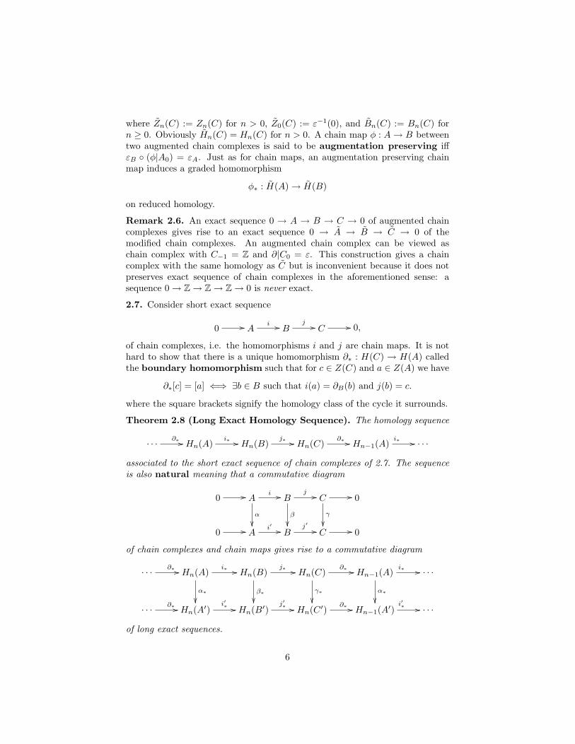
Theorem 2.8 (Long Exact Homology Sequence). The homology sequence

· · · ∂∗ // Hn(A)i∗ // Hn(B)

j∗ // Hn(C)∂∗ // Hn−1(A)

i∗ // · · ·associated to the short exact sequence of chain complexes of 2.7. The sequenceis also natural meaning that a commutative diagram

0 // Ai //

α

²²

Bj //

β

²²

C //

γ

²²

0

0 // Ai′ // B

j′ // C // 0

of chain complexes and chain maps gives rise to a commutative diagram

· · · ∂∗ // Hn(A)i∗ //

α∗²²

Hn(B)j∗ //

β∗²²

Hn(C)∂∗ //

γ∗²²

Hn−1(A)i∗ //

α∗²²

· · ·

· · · ∂∗ // Hn(A′)i′∗ // Hn(B′)

j′∗ // Hn(C ′)∂∗ // Hn−1(A′)

i′∗ // · · ·of long exact sequences.

6

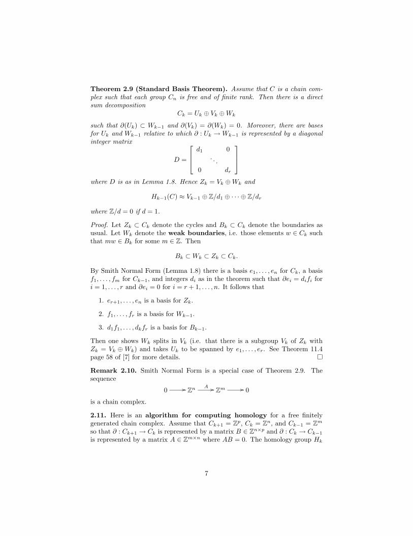
Theorem 2.9 (Standard Basis Theorem). Assume that C is a chain com-plex such that each group Cn is free and of finite rank. Then there is a directsum decomposition

Ck = Uk ⊕ Vk ⊕Wk

such that ∂(Uk) ⊂ Wk−1 and ∂(Vk) = ∂(Wk) = 0. Moreover, there are basesfor Uk and Wk−1 relative to which ∂ : Uk → Wk−1 is represented by a diagonalinteger matrix

D =

d1 0. . .

0 dr

where D is as in Lemma 1.8. Hence Zk = Vk ⊕Wk and

Hk−1(C) ≈ Vk−1 ⊕ Z/d1 ⊕ · · · ⊕ Z/dr

where Z/d = 0 if d = 1.

Proof. Let Zk ⊂ Ck denote the cycles and Bk ⊂ Ck denote the boundaries asusual. Let Wk denote the weak boundaries, i.e. those elements w ∈ Ck suchthat mw ∈ Bk for some m ∈ Z. Then

Bk ⊂ Wk ⊂ Zk ⊂ Ck.

By Smith Normal Form (Lemma 1.8) there is a basis e1, . . . , en for Ck, a basisf1, . . . , fm for Ck−1, and integers di as in the theorem such that ∂ei = difi fori = 1, . . . , r and ∂ei = 0 for i = r + 1, . . . , n. It follows that

1. er+1, . . . , en is a basis for Zk.

2. f1, . . . , fr is a basis for Wk−1.

3. d1f1, . . . , dkfr is a basis for Bk−1.

Then one shows Wk splits in Vk (i.e. that there is a subgroup Vk of Zk withZk = Vk ⊕ Wk) and takes Uk to be spanned by e1, . . . , er. See Theorem 11.4page 58 of [7] for more details.

Remark 2.10. Smith Normal Form is a special case of Theorem 2.9. Thesequence

0 // Zn A // Zm // 0

is a chain complex.

2.11. Here is an algorithm for computing homology for a free finitelygenerated chain complex. Assume that Ck+1 = Zp, Ck = Zn, and Ck−1 = Zm

so that ∂ : Ck+1 → Ck is represented by a matrix B ∈ Zn×p and ∂ : Ck → Ck−1

is represented by a matrix A ∈ Zm×n where AB = 0. The homology group Hk

7

is the quotient of the kernel of A by the image of B. Assume w.l.o.g. that B isin Smith Normal Form

B =[

D 0r×(p−r)

0(n−r)×r 0(n−r)×(p−r)

], D =

d1 0. . .

0 dr

.

Then as D is invertible over Q and AB = 0 the matrix A must have the form

A =[

0m×r A′], A′ ∈ Zm×(n−r).

The rank of A equals the rank of A′ so the nullity of A′ is ν := n− r− rank(A).The homology is

Ker(A)Im(B)

≈ Zν ⊕ Z/d1 ⊕ · · · ⊕ Z/dr.

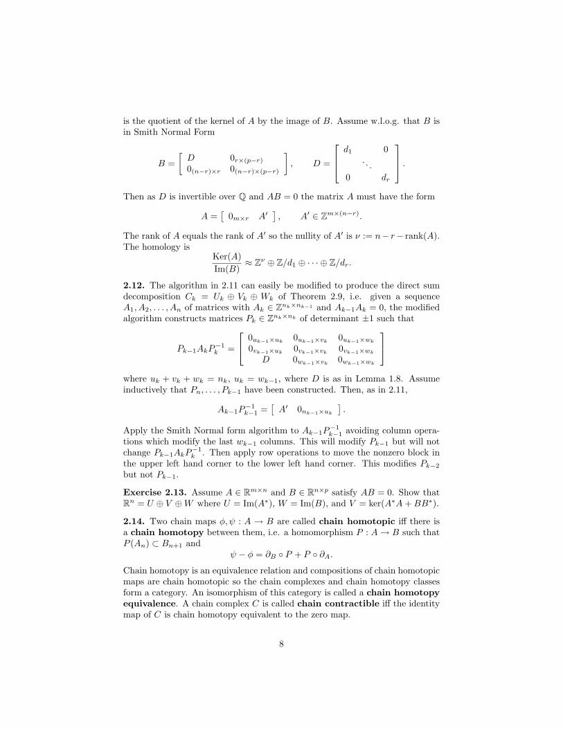
2.12. The algorithm in 2.11 can easily be modified to produce the direct sumdecomposition Ck = Uk ⊕ Vk ⊕ Wk of Theorem 2.9, i.e. given a sequenceA1, A2, . . . , An of matrices with Ak ∈ Znk×nk−1 and Ak−1Ak = 0, the modifiedalgorithm constructs matrices Pk ∈ Znk×nk of determinant ±1 such that

Pk−1AkP−1k =

0uk−1×uk0uk−1×vk

0uk−1×wk

0vk−1×uk0vk−1×vk

0vk−1×wk

D 0wk−1×vk0wk−1×wk

where uk + vk + wk = nk, uk = wk−1, where D is as in Lemma 1.8. Assumeinductively that Pn, . . . , Pk−1 have been constructed. Then, as in 2.11,

Ak−1P−1k−1 =

[A′ 0nk−1×uk

].

Apply the Smith Normal form algorithm to Ak−1P−1k−1 avoiding column opera-

tions which modify the last wk−1 columns. This will modify Pk−1 but will notchange Pk−1AkP−1

k . Then apply row operations to move the nonzero block inthe upper left hand corner to the lower left hand corner. This modifies Pk−2

but not Pk−1.

Exercise 2.13. Assume A ∈ Rm×n and B ∈ Rn×p satisfy AB = 0. Show thatRn = U ⊕ V ⊕W where U = Im(A∗), W = Im(B), and V = ker(A∗A + BB∗).

2.14. Two chain maps φ, ψ : A → B are called chain homotopic iff there isa chain homotopy between them, i.e. a homomorphism P : A → B such thatP (An) ⊂ Bn+1 and

ψ − φ = ∂B ◦ P + P ◦ ∂A.

Chain homotopy is an equivalence relation and compositions of chain homotopicmaps are chain homotopic so the chain complexes and chain homotopy classesform a category. An isomorphism of this category is called a chain homotopyequivalence. A chain complex C is called chain contractible iff the identitymap of C is chain homotopy equivalent to the zero map.

8

Theorem 2.15. If two chain maps φ, ψ : A → B are chain homotopic, theyinduce the same map on homology, i.e. φ∗ = ψ∗ : H(A) → H(B).

Proof. Assume that φ−ψ = ∂BP +P∂A. If ∂Ax = 0 then φ(x) = ψ(x)+∂BPxso φ∗[x] = ψ∗[x].

3 Singular Homology

3.1. Let X be a topological space. A map σ : ∆n → X is called a singularn-simplex in X. The free Abelian group generated by the singular n-simplicesis denoted by Cn(X) and its elements are called singular n-chains. A singularn-chain c is a finite formal sum of singular n-simplices, i.e.

c ∈ Cn(X) ⇐⇒ c =r∑

k=1

ckσk

where each σk is a singular n-simplex and ck ∈ Z. The boundary operator∂ : Cn(X) → Cn−1(Y ) is defined by

∂σ =n∑

i=0

(−1)kσ ◦ ιk

where ιk : ∆n−1 → ∆n is defined by

ιk(x1, . . . , xn) = (x1, . . . , xk−1, 0, xk, . . . , xn).

It is easy to see that the sequence

· · · ∂ // Cn+1∂ // Cn

∂ // Cn−1∂ // · · ·

is a chain complex, i.e. that ∂2 = 0. We write

C(X) :=⊕

n∈ZCn(X)

where Cn(X) := 0 for n < 0. The cycles of this complex are denoted byZ(X) and the boundaries by B(X). As usual Zn(X) := Z(X) ∩ Cn(X) andBn(X) := B(X) ∩ Cn(X). The quotient

H(X) :=⊕

n

Hn(X), Hn(X) := Zn(X)/Bn(X)

is called the singular homology group of the space X.

3.2. Let A ⊂ X be a subspace of X. Then C(A) is a subcomplex of C(X). Thequotient complex is denoted

C(X, A) :=⊕

n

Cn(X, A), Cn(X, A) := Cn(X)/Cn(A).

9

Elements of the groups

Zn(X, A) := ∂−1Cn(A), Bn(X, A) := Bn(X) + Cn(A)

are called relative singular cycles and relative singular boundaries re-spectively. The homology

H(X, A) :=⊕

n

Hn(Z, A), Hn(X, A) := Zn(X, A)/Bn(X,A)

is called the relative singular homology of the pair (X, A).

3.3. The standard augmentation ε : C0(X) → Z of the singular chain com-plex C(X) is defined by

ε

(∑

i

cipi

)=

∑

i

ci.

Here we identify the point p ∈ X with the singular simplex ∆0 → X : 1 7→ p.(Recall that ∆0 = {1}.) The corresponding reduced homology group is denotedH(X) and is called the reduced singular homology group of X. Thus

H(X) =⊕

n

Hn(X)

where Hn(X) = Hn(X) for n > 0 and

H0(X) =ε−1(0)B0(X)

⊂ H0(X).

3.4. A map f : X → Y induces a homomorphism

f# : Cn(X) → Cn(Y )

defined by f#(σ) := f ◦σ for each singular n-simplex in X. This homomorphismis a chain map, i.e. f# ◦ ∂ = ∂ ◦ f#. This implies that f#(Bn(X)) ⊂ Bn(Y )and f#(Zn(X)) ⊂ Zn(Y ). Hence f induces a map

f∗ : H(X) → H(Y ).

The chain map preserves the standard augmentation so f∗(Hn(X)) ⊂ Hn(Y ).Moreover, if f : (X, A) → (Y, B) then f#(Cn(A)) ⊂ Cn(B) so f induces a mapf∗ : Hn(X, A) → Hn(Y,B) on relative homology.

Remark 3.5. The three constructions H(X), H(X, A), and H(X) determineone another as follows. The unique map q : X → {∗} from the space X to theone point space gives a set theoretic equality

H(X) = Ker(q∗) ⊂ H(X).

10

For p ∈ X the sequence {p} → X → {p} gives a splitting

H(X) = H(X)⊕H({p}).The composition C(X) → C(X) → C(x, {p}) induces an isomorphism

H(X) ≈ H(X, {p}).In Corollary 5.7 below we will prove that for “nice pairs” (X,A) the projection(X, A) → (X/A,A/A) induces an isomorphism

H(X,A) ≈ H(X/A,A/A) ≈ H(X/A).

Note the obvious identification X → X/∅. The empty sum is zero so C(∅) ={0}. The map C(X) → C(X, ∅) : c 7→ c + {0} = {c} gives a correspondingisomorphism

H(X) = H(X, ∅).Theorem 3.6 (Dimension Axiom). If X is a point p, then Hn(X) = 0 forn > 0 and H0(X) = Z.

Proof. Cn(p) = Z for n ≥ 0 and ∂|Cn(p) = 0 or the identity according as n isodd or even.

Proposition 3.7. If X is pathwise connected, then H0(X) = Z.

Proposition 3.8. Let {Xα}α∈Λ be the path components of X. Then Hn(X) =⊕α∈Λ Hn(Xα).

Proof. Zn(X) =⊕

α∈Λ Zn(Xα) and Bn(X) =⊕

α∈Λ Bn(Xα).

Theorem 3.9 (Homotopy Axiom). If f, g : X → Y are homotopic, then thechain maps f# and g# are chain homotopic so f∗ = g∗.

Proof. Let F : X × I → Y satisfy F (x, 0) = f(x) and F (x, 1) = g(x). Definethe prism operator P : Cn(X) → Cn+1(Y ) by

P (σ)(x0, . . . , xn) =n+1∑

k=0

(−1)kF (σ(x0, . . . , xn), x0 + · · ·+ xk−1

)

for each singular n-simplex σ in X. The prism operator is a chain homotopy.The geometric interpretation is that the prism ∆n × I is written as a union of(n + 1)-simplices

∆n × I =n⋃

k=0

[v0, . . . , vk, wk, . . . , wn]

where vi = (ui, 0), wi = (ui, 1), ui are the vertices ∆n, and [. . .] denotes convexhull. The formula ∂P = g# − f# + P∂ expresses the boundary of the prism asthe top minus the bottom minus the prism on the faces of ∆n. The internalfaces of the decomposition cancel. See [3] page 112.

11

4 Simplicial Homology

In this section we define two subcomplexes ∆(X) and ∆′(X) of the singularchain complex C(X) of a ∆-complex X and state analogs of the basic theoremsin homology theory. The analogs are easier to understand than the correspond-ing theorems on singular theory since the subcomplexes are finitely generated.In section 6 we present a more general theory which makes singular homologyeven easier to compute. The inclusions

∆(X) → ∆′(X) → C(X)

induce isomorphisms in homology.

4.1. Let {Φα : Dα → X}α∈Λ be a ∆-complex. Each characteristic map Φα :∆n → X may be viewed as a singular n-simplex: denote by ∆n(X) the subgroupof the singular chain group Cn(X) generated by the characteristic maps. Bythe definition of ∆-complex there is a function β = β(α, k) which assigns to theindex α the (unique) index β such that Φβ = Φα ◦ ιk where ιk : ∆n−1 → ∆n isinclusion into the kth face. Hence

∂Φα =n∑

k=0

(−1)kΦβ(α,k)

which shows that∆(X) :=

⊕

n∈N∆n(X)

is a subcomplex of the singular chain complex C(X). The homology

H∆(X) =⊕

n∈NH∆

n (X)

of this subcomplex is called the simplicial homology of the ∆-complex X.Thus

H∆n (X) := Z∆

n (X)/B∆n (X)

where Z∆n (X) := ∆n(X) ∩ Zn(X) and B∆

n (X) := ∂(∆n+1(X)). The inclusion∆(X) → C(X) is a chain map and induces a homomorphism H∆(X) → H(X).Theorem 4.21 below asserts that this homomorphism is an isomorphism.

Example 4.2. The torus T 2 is the surface obtained from the unit square I2with the identifications (x, 0) ∼ (x, 1) and (0, y) ∼ (1, y). The Klein bottleK2 is the surface obtained from the unit square I2 with the identifications(x, 0) ∼ (x, 1) and (0, y) ∼ (1, 1− y). The projective plane P 2 is the surfaceobtained from the unit square I2 with the identifications (x, 0) ∼ (1− x, 1) and(0, y) ∼ (1, 1− y). For X = T 2,K2, P 2 there is a ∆-complex Φ as indicated inFigure 1. For X = T 2 and X = K2 there are one 0-simplex v, three 1-simplicesa, b, c, and two 2-simplices U and L. For X = P 2 we must adjoin another0-simplex w. In each case the bijections Φα is determined by the diagram in

12

6¡

¡¡µ-

6

-

¡¡

¡¡

¡

v

v

v

v

U

La a

b

b

c

T 2

6¡

¡¡µ-

?

-

¡¡

¡¡

¡

v

v

v

v

U

La a

b

b

c

K2

6¡

¡¡µ-

?

¾

¡¡

¡¡

¡

v

w

w

v

U

La a

b

b

c

P 2

Figure 1: Three ∆-complexes

the only way possible so that the corresponding maps to I2 are affine and thearrows on the edges match up. Note that had we reversed the arrows marked ain P 2 the vertices of triangle U would be cyclically (not linearly) ordered. Thefigure would still represent the projective plane but not a ∆-complex.

Proposition 4.3. The simplicial homology of the ∆-complex for the torus T 2

isH∆

2 (T 2) = Z, H∆1 (T 2) = Z2, H∆

0 (T 2) = Z

with H∆n (T 2) = 0 for n > 2.

Proof. The chain groups are ∆2(T 2) = Z2 with generators U,L, ∆1(T 2) =Z3 with generators a, b, c, and ∆0(T 2) = Z with generator v. The boundaryoperator is given by

∂U = b− c + a, ∂L = a− c + b, ∂a = ∂b = ∂c = 0.

Using row and column operations we find the Smith Normal Form for the matrixrepresenting ∂ : ∆2(T 2) → ∆1(T 2) is

B := P

1 11 1

−1 −1

Q−1 =

1 00 00 0

and the matrix representing ∂ : ∆1(T 2) → ∆0(T 2) is of course

A :=[

0 0 0].

In the notation of 2.11 ν := n − r − rank(A) = 3 − 1 − 0 = 2 so H∆1 (T 2) =

Zν ⊕ Z/1 = Z2. From B2 = 0 and rank(B) = 1 we get H∆2 (T 2) = Z∆

2 (T 2) = Zand from A = 0 we get H∆

0 (T2) = ∆0(T 2) = Z.

Proposition 4.4. The simplicial homology of the ∆-complex for the Klein bottleK2 is

H∆2 (K2) = 0, H∆

1 (K2) = Z⊕ (Z/2), H∆0 (K2) = Z

with H∆n (P 2) = 0 for n > 2.

13

Proof. The chain groups are as for T 2 but the boundary operator is given by

∂U = b− c + a, ∂L = a− b + c, ∂a = ∂b = ∂c = 0.

Using row and column operations we find the Smith Normal Form for the matrixrepresenting ∂ : ∆2(K2) → ∆1(K2) is

B := P

1 11 −1

−1 1

Q−1 =

1 00 20 0

and the matrix representing ∂ : ∆1(K2) → ∆0(K2) is again A = 01×3. Inthe notation of 2.11 ν := n − r − rank(A) = 3 − 2 − 0 = 1 so H∆

1 (K2) =Zν ⊕ (Z/1) ⊕ (Z/2) = Z ⊕ (Z/2). From B2 = 0 and rank(B) = 2 we getH∆

2 (K2) = Z∆2 (K2) = 0 and H∆

0 (K2) = Z as for T 2.

Proposition 4.5. The simplicial homology of the ∆-complex for the projectiveplane P 2 is

H∆2 (P 2) = 0, H∆

1 (P 2) = Z/2, H∆0 (P 2) = Z

with H∆n (P 2) = 0 for n > 2.

Proof. The chain groups are ∆2(P 2) = Z2 and ∆1(P2) = Z3 as before but∆0(P 2) = Z2 with generators v and w. The boundary operator is given by

∂U = b− a + c, ∂L = a− b + c, ∂a = ∂b = w − v, ∂c = 0.

Using row and column operations we find the Smith Normal Form for the matrixrepresenting ∂ : ∆2(T 2) → ∆1(T 2) is

B := P

1 11 −1

−1 1

Q−1 =

1 00 20 0

and the matrix representing ∂ : ∆1(P 2) → ∆0(P 2) is

A =[

1 1 0−1 −1 0

].

In the notation of 2.11 ν := n − r − rank(A) = 3 − 2 − 1 = 0 so H∆1 (P 2) ≈

Zν ⊕ (Z/1) ⊕ (Z/2) = Z/2. As for K2 we have H∆2 (P 2) = Z∆

2 (P 2) = 0. TheSmith normal form for A is

M

[1 1 0

−1 −1 0

]N−1 =

[1 0 00 0 0

]

so B∆0 (P 2) ≈ Z× 0 ⊂ Z2 = ∆0(P 2) =: Z∆

0 (P 2) and hence H∆0 (P 2) = Z.

14

4.6. The standard n-simplex ∆n is itself a simplicial complex with a character-istic map Φα : ∆k → ∆n for each subset α = {α0, α1, . . . , αk} ⊂ {0, 1, . . . , n},(α0 < α1 < · · · < αk), namely φα(x) = y where xi = yαi

for i = 0, 1, . . . , k andyj = 0 for j /∈ α. The space ∆n is homeomorphic to the disk Dn, its boundary

Σn−1 := {x ∈ ∆n : some xi 6= 0}is a subcomplex of ∆n homeomorphic to the sphere Sn−1.

Proposition 4.7. The ∆-homology of ∆n is given by

H∆0 (∆n) = Z, H∆

k (∆n) = 0 for k 6= 0.

The ∆-homology of Σn−1 is given by

H∆0 (Σn−1) = H∆

n−1(Σn−1) = Z, H∆

k (∆n) = 0 for k 6= 0, n.

The boundary ∂id∆n of the identity map of ∆n (viewed as an element of ∆n−1(Σn−1))gives a generator of H∆

n−1(Σn−1).

Proof. Define a chain homotopy Kk : ∆k(∆n) → ∆k+1(∆n) by

Kk(Φα) =

{Φ{0}∪α if 0 /∈ α,0 if 0 ∈ α,

so Kk∂ +∂Kk+1 = id and ∂K0 = id−Φ{0}. Also K : ∆k(Σn−1) → ∆k+1(Σn−1)for k < n and the complexes ∆(∆n) and ∆(Σn−1) are the same except that∆n(∆n) = Z and ∆n(Σn−1) = 0.

4.8. Let {Φα : Dα → X}α∈Λ be a ∆-complex and ∆′k(X) ⊂ Ck(X) be the

subgroup of the nth singular chain group of X generated by all maps of formΦα ◦ g where Φα : ∆n → X is a characteristic map of the ∆-complex X andg : ∆k → ∆n is simplicial, i.e. it sends each vertex vi of ∆k to a vertex g(vi) of∆n and preserves convex combinations. Then

∆′(X) :=⊕

n∈N∆′

n(X)

is a subcomplex of the singular chain complex. We denote by

H∆′(X) =⊕

n∈NH∆′

n (X)

the homology of this subcomplex. Thus

H∆′n (X) := Z∆′

n (X)/B∆′n (X)

where Z∆′n (X) := ∆′

n(X)∩Zn(X) and B∆′n (X) := ∂(∆′

n+1(X)). The chain mapf# : C(X) → C(Y ) induced by a ∆-map f : X → Y satisfies

f#(∆′(X)) ⊂ ∆′(Y ).

15

Thus H∆′ defines a functor from the category of ∆-complexes to the categoryof chain groups. By contrast, usually f# will not map ∆(X) to ∆(Y ) an so theoperation H∆ is not obviously functorial. However H∆ has the advantage thatit is much easier to compute since the group ∆n(X) has much lower rank thanthe group ∆′

n(X).

4.9. For a ∆-complex the standard augmentation ε : C0(X) → Z of 3.3 restrictsto augmentations of ∆(X) and ∆′(X). The corresponding reduced chain groupsare denoted by ∆(X) and ∆′(X) so that ∆n(X) = ∆n(X) and ∆′

n(X) = ∆′n(X)

for n > 0 and

∆0(X) = ∆′0(X) =

{ ∑

x∈X0

cxx :∑

x∈X0

cx = 0

}

where the sums are understood to be finite even if X0 is infinite. The corre-sponding reduced homology groups are denoted H∆(X) and H∆′(X).

4.10. Let (X,A) be a ∆-pair and define the quotient chain complexes

C∆(X, A) := C∆(X)/C∆(A), C∆′(X, A) := C∆′(X)/C∆′(A).

The homology groups of these complexes are denoted respectively H∆(X, A)and H∆′(X, A).

Theorem 4.11. Let X be a ∆-complex. Then the inclusion φ : ∆(X) → ∆′(X)is a chain homotopy equivalence.

Proof. Equip the vertices of the standard simplex ∆n with the lexicographicalordering i.e. where vi denotes the vertex with 1 in the ith place and 0 elsewherewe have vi < vj ⇐⇒ i < j. An injective simplicial map g : ∆k → ∆n

determines a unique simplicial automorphism σ of ∆k such that g ◦ σ is anorder preserving embedding from the vertices of ∆k to the vertices of ∆n. Letsgn(σ) denote the sign of the corresponding permutation of the vertices. Defineψ : ∆′(X) → ∆(X) by

ψ(Φα ◦ g) =

{sgn(σ)Φα(g ◦ σ) if g is injective0 otherwise.

Then ψ is a chain map, ψ ◦ φ is chain homotopic to the identity of ∆(X), andφ ◦ ψ is chain homotopic to the identity of ∆′(X). See [7] page 77.

Exercise 4.12. Let p be a point viewed as a ∆-complex in the only way possible.Show that H∆

n (p) = H∆′n (p) = 0 for n > 0 and H∆

0 (p) = H∆′0 (p) = Z. Hence

H∆(p) = H∆′(p) = 0.

Exercise 4.13. Two ∆-maps f, g : X → Y are said to be ∆-homotopic iffthere is a ∆-map F : X × I → Y such that F (·, 0) = f and F (·, 1) = g. HereX × I is the product ∆-complex described in Theorem 2.10 on page 111 of [3].Show that If two ∆-maps f, g : X → Y are ∆-homotopic, then the inducedmaps f#, g# : ∆′(X) → ∆′(Y ) are ∆-homotopic.

16

Exercise 4.14. Let (X,A) be a ∆-pair, i : A → X denote the inclusion, andp : X → X/A denote the projection. Show that the sequence

0 // ∆(A)i# // ∆(X)

p# // ∆(X/A) // 0

is exact. This gives a long exact sequence

· · · ∂ // H∆k (A)

i# // H∆k (X)

p# // H∆k (X/A)

∂ // H∆k−1(A)

i# // · · ·

Exercise 4.15. Continue the notation of 4.14. The exact sequence

0 // ∆(A)i# // ∆(X)

p# // ∆(X)/∆(A) // 0

is exact and gives a long exact sequence

· · · ∂ // H∆k (A)

i# // H∆k (X)

p# // H∆k (X, A) ∂ // H∆

k−1(A)i# // · · ·

Remark 4.16. For a finite zero-dimensional ∆-complex (i.e. a finite set) Xthe exact sequence of 4.15 is

0 → Z#(A) → Z#(X) → Z#(X)−#(A) → 0

and the exact sequence of Theorem 4.14 is

0 → Z#(A)−1 → Z#(X)−1 → Z#(X)−#(A) → 0.

Exercise 4.17. Let (X, A) be a ∆-pair and Z ⊂ A be an open subset of Xsuch that A \ Z is a subcomplex of A. Then X \ Z is a subcomplex of X andthe inclusion (X \ Z,A \ Z) ⊂ (X,A) induces an isomorphism

H∆(X \ Z, A \ Z) ≈ H∆(X, A).

This might be called the Excision Theorem for simplicial homology.

Exercise 4.18. In the situation of 4.17 the map

(X \ Z)/(A \ Z) → X/A

induced by the inclusion is a ∆-isomorphism and thus induces an isomorphismH∆

((X \ Z)/(A \ Z)

) → H∆(X/A). Show that this is the same as the isomor-phism obtained by combining the isomorphisms of 4.17 and 4.15.

Exercise 4.19. Let A and B be subcomplexes of a ∆-complex X. Then A∩Band A ∪B are also subcomplexes. Show that there is an exact sequence

· · · → H∆n (A ∩B) → H∆

n (A)⊕H∆n (B) → H∆

n (A ∪B) → H∆n−1(A ∩B) → · · ·

17

This might be called the Mayer Vietoris Theorem for simplicial homology.Hint: The sequence

0 → ∆(A) ∩∆(B) → ∆(A)⊕∆(B) → ∆(A ∪B) → 0

is exact. The map ∆(A)∩∆(B) = ∆(A∩B) → ∆(A)⊕∆(B) is the direct sumof the inclusions and the map ∆(A)⊕∆(B) → ∆(A∪B) is the difference of theinclusions of the summands.

Remark 4.20. For a finite zero-dimensional ∆-complex (i.e. a finite set) Xthe exact sequence of 4.19 is

0 → Z#(A∩B) → Z#(A) ⊕ Z#(A) → Z#(A∪B) → 0

which shows that the Mayer Vietoris Theorem is a generalization of the Inclusion-Exclusion Principle of combinatorics.

Theorem 4.21. Let X be a ∆-complex. Then the inclusion ∆(X) → C(X)induces an isomorphism H∆(X) → H(X) between simplicial homology and sin-gular homology.

Proof. This is proved for the k-skeleton X(k) by induction on k, the long exactsequences (in both homology theories) for the pair (X(k), X(k−1)), and the FiveLemma 1.14. See [3] Page 128.

5 Subdivision

5.1. For a ∆-pair (X, A) the sequence

0 → ∆(A) → ∆(X) → ∆(X/A) → 0

is exact and induces a long exact sequence in simplicial homology. The analogoussequence

0 → C(A) → C(X) → C(X/A) → 0

in singular theory is not exact. For example, if X = I2, A = {12} × I, and

σ ∈ C1(X/A) is defined by σ(t) = (0, t) for t < 12 and σ(t) = (1, t) for t > 1

2then σ does not lift to X. This nonexactness is the main reason why the relativehomology groups H(X,A) are used in place of the reduced homology groupsH(X/A). Corollary 5.7 asserts that H(X,A) and H(X/A) are isomorphic. Theproof requires the following

Theorem 5.2. Let X be a topological space and U = {Uλ}λ∈Λ be a collectionof subsets of X whose interiors cover X. Let CU (X) be the subcomplex of thesingular chain complex of X generated by the singular simplices σ : ∆n → Xsuch that σ(∆n) ⊂ Uλ for some λ ∈ Λ and let HU (X) denote the homology ofthis subcomplex. Then the inclusion CU (X) → C(X) induces an isomorphismHU (X) → H(X).

18

5.3. Fix a convex subset K of Rm. Denote by LC(K) the subcomplex of thesingular chain complex C(K) generated by all singular simplices σ : ∆n → Rm

of form

σ(t0, t1, . . . , tn) =n∑

i=0

tiwi

where w0, w1, . . . , wn ∈ K. The singular simplex σ is called the linear simplexwith vertices w0, w1, . . . , wn. The elements of LC(K) are called linear singularchains. Each point b ∈ K determines a cone operator b : Cn(K) → Cn+1(K)denoted by the same symbol via the formula

b(σ)(s−1, s0, s1, . . . , sn) = s−1b +n∑

i=0

siwi.

For each linear n-simplex σ the point

bσ :=1

n + 1

n∑

i=0

wi

is called the barycenter of σ. The map S : LCn(K) → LCn(K) definedinductively by

S([w]) = [w], S(σ) = bσ(S∂σ)

is called linear barycentric subdivision.

Lemma 5.4. The map S is a chain map and is chain homotopic to the identity,i.e. there are maps T : LCn(K) → LCn+1(K) such that

∂T + T∂ = id− S.

Proof. See [3] page 121-2.

5.5. We now specialize to the K = ∆n the standard n-simplex. Denote the ver-tices of ∆n of v0, v1, . . . , vn. For a set I ⊂ {0, 1, . . . , n} of indices let ∆I denotethe convex hull of {vi : i ∈ I}. Each permutation α of {0, 1, . . . , n} determinesa linear simplex σα ∈ LCn(∆n) whose kth vertex wk is the barycenter of ∆Ik

where Ik = {α(0), . . . , α(k)}. Let idn denote the identity map of ∆n viewed asa linear simplex. Then

idn =⋃α

εασα

where εα = ±1; the choice of these signs assures that the internal faces cancel. Inparticular, ∆n =

⋃α σα(∆n) and the interiors (in ∆n) of the simplices σα(∆n)

are pairwise disjoint. The chain homotopy T is determined by the formula

T (idn) = p#

(τ +

∑α

εατα

)

19

where p : ∆n × I→ ∆n is projection on the first factor and τ : ∆n+1 → ∆n × Iare linear simplex whose vertices are (b, 1) [here b is the barycenter of ∆n] and(vi, 0) for i = 0, . . . , n and where τα : ∆n+1 → ∆n × I is the linear simplexwhose vertices are (vα(0), 0) and (vα(i), 1) for i = 0, . . . , n. See [3] page 122.

Proof of Theorem 5.2. Let X be any topological space. Define a chain mapS : Cn(X) → Cn(X) and a chain homotopy T : Cn(X) → Cn+1(X) by

S(σ) = σ#(S(idn)), T (σ) = σ#(T (idn)).

The formula ∂T + T∂ = id − S holds so S is chain homotopic to the identityid. By induction and the fact that compositions of chain homotopic maps arechain homotopic we have that the mth iterate Sm of S is chain homotopic tothe identity, in fact

∂Dm + Dm∂ = id− Sm

where Dm =∑

i<m TSi. Etc.

Corollary 5.6 (Excision). Let X be any topological space and Z ⊂ A ⊂ X besuch that the closure of Z is a subset of the interior of A. Then the inclusion(X \ Z, A \ Z) → (X, A) induces an isomorphism

H(X \ Z,A \ Z) ≈ H(X, A)

of the relative homology groups.

Proof. Let U = {X \ Z, A}. The map C(X \ Z)/C(A \ Z) → CU (X)/C(A) isan isomorphism and the map CU (X)/C(A) → C(X)/C(A) induces an isomor-phisms in homology by Theorem 5.2. Hence

H(X \ Z,A \ Z) ≈ HU (X, A) ≈ H(X, A)

where HU (X, A) denotes the homology of CU (X)/C(A). See page 124 of [3].

Corollary 5.7. Assume that (X, A) is a nice pair, i.e. that A has a neigh-borhood V in X which deformation retracts onto A. Then the projection

(X, A) → (X/A,A/A)

induces an isomorphism is relative homology and hence

H(X,A) ≈ H(X/A,A/A) ≈ H(X/A).

Proof. In the commutative diagram

H(X, A)

²²

// H(X,V )

²²

H(X \A, V \A)oo

²²H(X/A,A/A) // H(X/A, V/A) H(X/A \A/A, V/A \A/A)oo

the horizontal maps on the left are isomorphisms by homotopy, the horizontalmaps on the right are isomorphisms by excision, the vertical map on the rightis an isomorphism as it is induced by a homeomorphism, and hence the othertwo vertical maps are isomorphisms. See Proposition 2.22 page 124 of [3].

20

Corollary 5.8 (Mayer Vietoris). Let X be any topological space and A,B ⊂X be two subsets whose interiors cover X. Then there is an exact sequence

· · · → Hn(A ∩B) → Hn(A)⊕Hn(B) → Hn(X)∂∗ // Hn−1(A ∩B) → · · ·

where the map H(A∩B) → H(A)⊕H(B) is the direct sum of the maps inducedby the inclusions A∩B → A and A∩B → A, the map H(A)⊕H(B) → H(X)is the difference of the maps induced by the inclusions A → X and B → X, andthe boundary operator ∂∗ is defined in the proof.

Proof. The collection U = {A,B} satisfies the hypothesis of Theorem 5.2, and

0 → C(A ∩B) → C(A)⊕ C(B) → CU (X) → 0

is an exact sequence of chain complexes.

6 Cellular Homology

Definition 6.1. By Proposition 4.7 and Theorem 4.21 we have Hn(Sn) = Z.Hence each continuous map f : Sn → Sn determines an integer deg(f) calledthe degree of f via the equation

f∗[Sn] = deg(f)[Sn]

where [Sn] is a generator of Hn(Sn).

6.2. Now let Φ = {Φα : Dα → X}α∈Λ be a cell complex, nα be the dimensionof the disk Dα, Let

Cn(Φ) :=⊕

nα=n

ZΦα

be the free Abelian group generated by the n-dimensional cells of the complex.For each pair of indices α, β ∈ Λ with nβ = nα − 1 = n− 1 define

φαβ : ∂Dα = Sn−1 → Dβ/∂Dβ = Dn−1/Sn−2 ≈ Sn−1

by φαβ = Φ−1β ◦ qβ ◦ φα where φα = Φα|∂Dα is the attaching map, qβ :

X(n−1)/X(n−2) → eβ/X(n−2) is the identity on eβ and sends the complementof eβ to the wedge point, and Φ−1

β is induced by the inverse of the characteristicmap. Define ∂ : Cn(Φ) → Cn−1(Φ) by

∂Φα =∑

β

deg(φαβ)Φβ

Theorem 6.3. The homomorphism ∂ : C(Φ) → C(Φ) is a chain complex, i.e.∂2 = 0. The homology H(Φ) of this chain complex is isomorphic to the singularhomology H(X) of the space X.

21

Proof. See [3] pages 137-141. An important point is that for each n character-istic map Φ induces a homeomorphism

∨nα=n

Sα ≈ X(n)/X(n−1), Sα := Dα/∂Dα

from a wedge of n-spheres to the quotient of the n skeleton by the (n − 1)-skeleton. and that homeomorphism in turn induces an isomorphism

Cn(Φ) ' Hn(X(n)/X(n−1))

of Abelian groups.

Example 6.4. The standard representation P/∼ of the compact orientablesurface Mg of genus g (connected sum of g copies of the torus) is obtained froma 4g-gon P with boundary

∂P = α1 ∪ α2 ∪ β1 ∪ β2 ∪ · · · ∪ α2g−1 ∪ α2g ∪ β2g−1 ∪ β2g,

where the sides are enumerated and oriented in the clockwise direction andwhere αi and βi are identified by an orientation reversing homeomorphism.This gives a cell complex structure Φ whose cellular chain complex is

0 // Z 0 // Z2g 0 // Z // 0

so the homology is

H0(Mg) = Z, H1(Mg) = Z2g, H1(Mg) = Z.

See Example 2.36 page 141 of [3].

Example 6.5. The standard representation P/∼ of the compact nonorientablesurface Nk of genus k (connected sum of k copies of the projective plane) isobtained from a 2k-gon P with boundary

∂P = α1 ∪ β1 ∪ · · · ∪ αk ∪ βk,

where the sides are enumerated and oriented in the clockwise direction andwhere αi and βi are identified by an orientation preserving homeomorphism.This gives a cell complex structure Φ whose cellular chain complex is

0 // Z ∂ // Z2g 0 // Z // 0

where ∂(1) = (2, 2, . . . , 2) so the homology is

H0(Ng) = Z, H1(Ng) = Zg−1 ⊕ Z/2, H2(Ng) = 0.

See Example 2.37 page 141 of [3].

22

Example 6.6. The 3-torus T 3 = S1 × S1 × S1 may be viewed as a cube withopposite faces identified. This gives a cell complex structure Φ whose cellularchain complex is

0 // Z 0 // Z3 0 // Z3 0 // Z // 0

so the homology is

H0(T 3) = Z, H1(T 3) = Z3, H3(T 3) = Z3, H3(T 3) = Z.

See Example 2.39 page 142 of [3].

Example 6.7. The Moore Space See Example 2.40 page 143 of [3].

Example 6.8. The real projective space RPn See Example 2.41 page 144of [3].

Example 6.9. The complex projective space CPn

Example 6.10. The lens space Lm(p, q) See Example 2.42 page 144 of [3].

References

[1] Charles Conley: Isolated Inveariant Sets and the Morse Index, CBMS Con-ferences in Math 38, AMS 1976.

[2] William Fulton: Algebraic Topology, A First Course Springer GTM 153,1995.

[3] Allen Hatcher: Algebraic Topology, Cambridge U. Press, 2002.

[4] John G. Hocking & Gail S. Young: Topology, Addisow Wesley, 1961.

[5] Morris W. Hirsch: Differential Topology, Springer GTM 33, 1976.

[6] William S. Massey: A Basic Course in Algebraic Topology, Springer GTM127, 1991.

[7] James R. Munkres: Elements of Algebraic Topology, Addison Wesley, 1984.

[8] S. Shelah: Can the fundamental group of a space be the rationals? Proc.Amer. Math. Soc. 103 (1988) 627–632.

[9] Stephen Smale: A Vietoris mapping theorem for homotopy. Proc. Amer.Math. Soc. 8 (1957), 604–610

[10] J. W. Vick: Homology Theory (2nd edition), Graduate Tests in Math 145,Springer 1994.

[11] J.H.C. Whitehead: Combinatorial homotopy II, Bull. A.M.S 55 (1949)453-496.

[12] George W. Whitehead: Elements of Homotopy Theory Graduate Texts inMath 61, Springer 1978.

23