Homogenous Contracts for Heterogeneous Agents: AligningSalesforce Composition and Compensation∗

Øystein Daljord Sanjog Misra Harikesh S. Nair

Past versions: June 2012; Feb 2013. This version: Jan 2014

Abstract

Observed contracts in the real-world are often very simple, partly reflecting the con-straints faced by contracting firms in making the contracts more complex. We focus on onesuch rigidity, the constraints faced by firms in fine-tuning contracts to the full distribution ofheterogeneity of its employees. We explore the implication of these restrictions for the pro-vision of incentives within the firm. Our application is to salesforce compensation, in whicha firm maintains a salesforce to market its products. Consistent with ubiquitous real-worldbusiness practice, we assume the firm is restricted to fully or partially set uniform commis-sions across its agent pool. We show this implies an interaction between the composition ofagent types in the contract and the compensation policy used to motivate them, leading toa “contractual externality” in the firm and generating gains to sorting. This paper explainshow this contractual externality arises, discusses a practical approach to endogenize agentsand incentives at a firm in its presence, and presents an empirical application to salesforcecompensation contracts at a US Fortune 500 company that explores these considerations andassesses the gains from a salesforce architecture that sorts agents into divisions to balancefirm-wide incentives. Empirically, we find the restriction to homogenous plans significantlyreduces the payoffs of the firm relative to a fully heterogeneous plan when it is unable tooptimize the composition of its agents. However, the firm’s payoffs come very close to thatof the fully heterogeneous plan when it can optimize both composition and compensation.Thus, in our empirical setting, the ability to choose agents mitigates the loss in incentivesfrom the restriction to uniform contracts. We conjecture this may hold more broadly.

∗Daljord : Graduate School of Business, Stanford University, daljord@stanford.edu; Misra: Ander-son School of Management, UCLA, sanjog.misra@anderson.ucla.edu; Nair : Graduate School of Busi-ness, Stanford University, harikesh.nair@stanford.edu. We thank Guy Arie, Nick Bloom, FrancineLafontaine, Ed Lazear, Sridhar Moorthy, Paul Oyer, Michael Raith, Kathryn Shaw, Chuck Weinberg,Jeff Zwiebel; our discussant at the QME conference, Curtis Taylor; and Lanier Benkard and Ed Lazearin particular for their useful comments and suggestions. We also thank seminar participants at MIT-Sloan, Stanford-GSB, UBC-Saunder, UC-Davis-GSM, UT-Austin-McCoombs, UToronto-Rotman, and atthe 2012 IOFest, Marketing Dynamics and QME conferences for useful feedback. The usual disclaimerapplies.

1

1 Introduction

In many interesting market contexts, firms face rigidities or constraints in fine-tuning theircontracts to reflect the full distribution of heterogeneity of the agents they are contractingwith. For example, auto-insurance companies are often prevented by regulation from con-ditioning their premiums on consumer characteristics like race and credit scores. Royaltyrates in business-format franchising in the US are typically constrained by norm to be thesame across all franchisees in a given chain.1 Wholesales contracts between manufacturersand downstream retailers in the US typically involve similar wholesales prices to all down-stream retailers within a given geographic area due to Robinson-Patman considerations.In salesforces, the context of the empirical example in this paper, incentive or commissionrates on output are invariably set the same across all sales-agents within a firm. For in-stance, a firm choosing a salary + commission salesforce compensation scheme typicallysets the same commission rate for every sales-agent on its payroll, in spite of the fact thatexploring the heterogeneity and setting an agent-specific commission may create theoret-ically better incentives at the individual level. While reasons are varied, full or partialuniformity of this sort is well documented to be an ubiquitous feature of real-world sales-force compensation (Rao 1990; Mantrala et al. 1994; Raju and Srinivasan 1996; Zoltnerset al. 2001; Lo et al. 2011).

The focus of this paper is on the implications to the principal of this restriction tosimilar contract terms across agents. We do not take a strong stance on the source of theuniformity, but focus on the fact that any such uniformity in the contract implies thatagents and contract terms have to be chosen jointly. In the salesforce context, for example,this creates an interaction between the composition of agent types in the contract and thecompensation policy used to motivate them, leading to a “contractual externality” in thefirm and generating gains to sorting. This paper explains how this contractual externalityarises, discusses a practical approach to endogenize agents and incentives at a firm, andpresents an empirical application to salesforce compensation contracts at a US Fortune500 company that explores these considerations and assesses the gains from a salesforcearchitecture that sorts agents into divisions to balance firm-wide incentives.

As a motivating example, consider a firm that has chosen a salary + commission scheme.Suppose all agents have the same productivity, but there is heterogeneity in risk aversionamongst the agents. The risk averse agents prefer that more of their pay arises from fixedsalary, but the less risk averse prefer more commissions. When commissions are restrictedto be uniform across agents, including the more risk averse types in the firm implies the

1Quoting Lafontaine and Blair (2009, pp. 395-396), “Economic theory suggests that franchisors shouldtailor their franchise contract terms for each unit and franchisee in a chain. In practice, however, contractsare remarkably uniform across franchisees at a point in time within chains [emphasis ours]..[]..a business-format franchisor most often uses a single business-format franchising contract—a single royalty rate andfranchise fee combination— for all of its franchised operations that join the chain at a given point..[]..Thus,uniformity, especially for monetary terms, is the norm.”

2

firm cannot offer high commissions. Dropping the bottom tail of agents from the firmmay then enable the firm to profitably raise commissions for the rest of agents. Knowingthat, the firm should choose agents and commissions jointly. This is our first point: therestriction to uniformity implies the composition and compensation are co-dependent. Toaddress this, we need to enlarge the contracting problem to allow the principal to choosethe distribution of types in his firm along with the optimal contract form given that typedistribution.

Our second point is that uniformity implies the presence of a sales-agent in the firmimposes an externality on the other agents in the pool through its effect on the shape of thecommon element of the incentive contract. For instance, suppose agents are homogenousin all respects except their risk aversion, and there are three agents, A, B and C who couldbe employed, with C the most risk averse. C needs more insurance than A and B andretaining him requires a lower common commission rate. It could then be that A and Bare worse off with C in the firm (lower commissions). Thus, the presence of the low-typeagent imposes an externality on the other sales-agent in the firm through the endogeneityof contract choice.

This externality can be substantial when agent types are multidimensional (for exam-ple, when agents are heterogeneous in risk aversion, productivity and costs of expendingsales effort). Consider the above example. It may be optimal for the principal to rankthe three agents on the basis of their risk aversion and to drop the “low-type” C from theagent pool. Hence, if risk aversion were the only source of heterogeneity, and we enlargethe contracting problem to allow the principal to choose both the optimal compositionand compensation, it may be that “low-types” like C impose little externalities becausethey are endogenously dropped from the firm. Now, consider what happens when typesare multidimensional. Suppose in addition to risk aversion, agents are heterogeneous intheir productivity (in the sense of converting effort into output), and C, the most riskaverse is the most productive. Then, the principal faces a tradeoff: dropping C from thepool enables him to set more high powered incentives to A and B, but also entails a largeloss in output because C is the most productive. In this tradeoff, it may well be that theoptimal strategy for the principal is to retain C in the agent-pool and to offer all the lowercommon commission induced by his presence. Thus multidimensional types increase thechance that the externalities we discussed above persist in the optimally chosen contract.More generally, multidimensionality of the type space also points to the need for a theoryto describe who should be retained and who should be let go from the salesforce, becauseagents cannot be ranked as desirable or undesirable on the basis of any one single variable.

Our main question explores the co-dependence between composition and compensation.We ask to what extent composition and compensation complement each other in realisticsalesforce settings. We use an agency theoretic set-up in which the principal chooses boththe set of agents to retain in the firm and the optimal contract to incentivize the retainedagents. We use our model to assess how contract form changes when the distribution of

3

ability changes. The answer to this is dependent on the distribution of heterogeneity inthe agent pool, and hence is inherently an empirical question.

We leverage access to a rich dataset containing the joint distribution of output andcontracts for all sales-agents at a Fortune 500 contact lens company in the US. FollowingMisra and Nair (2011), we use these data to identify primitive agent parameters (costof effort, risk aversion, productivity), and to estimate the multidimensional distributionof heterogeneity in these parameters across agents at the firm. In the data, agents arepaid according to a nonlinear, quarterly incentive plan consisting of a salary and a linearcommission which is earned if realized sales are above a contracted quota and below apre-specified ceiling. The nonlinearity of the incentive contract creates dynamics in theagent’s actions, causing the agent to optimally vary his effort profile as he moves closer toor above his quota. The joint distribution of output and the distance to the quota thusidentify “hidden” effort in this moral hazard setting. Following Misra and Nair (2011),we combine this identification strategy with a structural model of agent’s optimizationbehavior to recover the primitives underpinning agent types. We then use these estimatesas an input into a model of simultaneous contact form and agent composition choice forthe principal.

Solving this model involves computing a large-scale combinatorial optimization problemin which the firm chooses one of 2M possible salesforce configurations from amongst a poolofM potential agents, and solving for the optimal common incentive contract for the chosenpool. To find the optimal composition of agents, we can always enumerate the profits forall 2M combinations when M is small. If M is large, simple enumeration algorithm ispractically infeasible (M is around 60 in our focal firm, and could number in the hundredsor thousands in other applications). Since agents are allowed a multidimensional typespace, it is generally not possible to find a simple cut-off rule where agents above someparameter threshold are retained. Exploiting a characterization of the optimal solutionfor a class of composition-compensation problems, we derive an algorithm that allows usto search the exploding composition-compensation space by reducing the problem fromoptimization of a set-valued function to a standard optimization program for continuousfunctions on compact sets. The reduction makes the execution time of the algorithmindependent of the composition space itself. In examples we compute, we can search aspace of 25000 composition-compensations in fractions of a second. A power-set search ofa space of that size is otherwise prohibitive.

We use the algorithm to simulate counterfactual contracts and agent pools at theestimated parameters. We explore to what extent a change in composition of the agentsaffects the nature of optimal compensation for those agents, and quantify the profit impactof jointly optimizing over composition and compensation. We find that allowing the firmto optimize the composition of its types has bite in our empirical setting. When the firmis restricted to homogenous contracts and no optimization over types, we estimate itspayoffs are significantly lower than that under fully heterogeneous contracts. However,

4

the payoffs under homogeneous contracts when the firm can optimize both compositionand compensation come very close to that under fully heterogeneous contracts. Thus, theability to choose agents seems to help balance the loss in incentives from the restriction tohomogeneity. We conjecture this may be broadly relevant in other settings and may helprationalize the prevalence of homogenous contracts in many salesforce settings in spite ofthe profit consequences of reduced incentives.

We then simulate a variety of salesforce architectures in which the firm sorts its sale-sagents into divisions. We restrict each division to offer a uniform commission to all withinits purview, but allow commissions to vary across divisions. We then simultaneously solvefor the optimal commissions and the optimal allocation of agents to divisions. In the con-text of our empirical example, we find that a small number of divisions generates profitsto the principal that come very close to that under fully heterogeneous contracts. If thefirm is allowed to choose its composition as well, this profit gain is achieved with evenfewer divisions. The main take-away is that simple contracts combined with the ability tochoose agents seem to do remarkably well compared to more complex contracts, at leastin the context of our empirical example.

Our analysis is related to a literature that emphasizes the “selection” effect of incentives,for example, Lazear’s famous 2000a analysis of Safelite Glass Corporation’s incentive planfor windshield installers, in which he demonstrates that higher-ability agents remain withthe company after it switched from a straight salary to a piece-rate; or Bandiera et al.’s2007 analysis of managers at a fruit-picking company, who started hiring more high abilityworkers after they were switched to a contract in which pay depends on the performance ofthose workers. Lazear and Bandiera et al. present models of how the types of agents thatsort into or are retained at the firm changes in response to an exogenously specified piece-rate. In our set-up, the piece-rate itself changes as the set of agents at the firm changes,because the firm jointly chooses the contract and the agents. The endogenous adjustmentof the contract as the types change is key to our story. The closest we know to our pointin the literature is Lazear (2000b), who shows that firms may choose incentives to attractagents of high ability. Unlike our set-up though, Lazear considers unidimensional agentsin an environment with no asymmetric information or uncertainty. The broader point herethat piece-rates help manage heterogeneity within the firm is analogous to Lazear’s insight.

The literature on relative performance schemes and on teams (Holmstrom 1982; Kandeland Lazear 1992; Hamilton et al. 2003; Misra, Pinker and Shumsky 2004) has identifiedother contexts wherein one agent’s characteristics or actions substantively affects another’swelfare via an interaction with incentives. The contractual externality we identify persistswhen agents have exclusive territories and there are no across-agent complementarity orsubstitution effects in output, and is relevant even when contracts are absolute and notrelative. It is thus distinct from the mechanisms identified in this literature. A relatedliterature on contract design in which one principal contracts with many agents focuses onthe conditions where relative incentive schemes arise endogenously as optimal, and not on

5

the question of the joint choice of agents and incentives, which is our focus here. Broadlyspeaking, the relative incentive scheme literature focuses on the value of contracts in fil-tering out common shocks to demand and output, and on the advantages of contractingon the ordinal aspect of outputs when output is hard to measure (e.g, Lazear and Rosen1981; Green and Stokey 1983; Mookerjee 1984; Kalra and Shi 2001; Lim et al. 2009; Rid-lon and Shin 2010). Common shocks and noise in the output measure are not compellingfeatures of our empirical setting which involves selling of contact-lenses to optometricians,for which seasonality and co-movement in demand is limited, and sales (output) are pre-cisely tracked. A small theoretical literature also emphasizes why a principal may choose aparticular type of agent in order to signal commitment to a given policy (e.g., shareholdersmay choose a “visionary” CEO with a reputation for change-management so as to committo implementing change within the firm: e.g., Rotemberg and Saloner, 2000). Our point,that the principal may choose agents for incentive reasons, is distinct from that in thisliterature which focuses on commitment as the rationale of the principal for its choice ofagents. A related theoretical literature has also noted that contracts may signal informa-tion that affects the set of potential employees or franchisees a principal may contract with(Desai and Srinivasan 1995; Godes and Mayzlin 2012), without focusing on the principal’schoice of agents explicitly.

Our model predicts that agents and incentives across firms are simultaneously deter-mined and has implications for two related streams of empirical work. One stream mea-sures the effect of incentives on workers, and tests implications of contract theory usingdata on observed contracts and agent characteristics across firms (see Pendergast 1999 fora review). In an important contribution to the econometrics in this area, Ackerberg andBotticini (2002) note that when agents are endogenously matched to contracts, the correla-tion observed in data between outcomes and contract characteristics should be interpretedwith caution. A potential for confounds arises from unobserved agent characteristics thatmay potentially be correlated with both outcomes and contract forms. The resulting omit-ted variables problem may result in endogeneity biases when trying to measure the causaleffect of contracts on outcomes. Our model, which provides a rationale for why agentand contracts characteristics are co-determined across firms, has similar implications forempirical work using across-agent data. The model implies that the variation in contractterms across firms is endogenous to worker characteristics at those firms. While Ackerbergand Botticini (2002) stress the omitted variables problem, the endogeneity implied by ourmodel derives from the simultaneity of contracts and agents.

A second stream pertains to work that has measured complementarities in human re-source practices within firms, testing the theory developed in Milgrom and Roberts (1990)and Holmstrom and Milgrom (1994), amongst others. This theory postulates that humanresource activities like worker training and incentive provision are complementary activi-ties. A large body of empirical work has measured the extent of these complementaritiesusing across-firm data correlating worker productivity with the incidence of these activities

6

(e.g., Ichniowski, Shaw and Prennushi 1997 and others). Our model predicts that workersand incentives (or HR practices, more generally) are optimally jointly chosen. When bet-ter workers also have corresponding better productivity, the simultaneity of worker choiceand HR practices implies the incidence of HR practices are endogenous in productivityregressions, which confounds the measurement of such complementaries using across-firmdata. A related implication of our model is that endogenously adjusting common clausesof firm-wide contracts can generate across-agent dependencies in output that generate in-direct complementarities. If these are not accounted for, it may confound measurement ofother sources of direct complementarities like peer effects that researchers are interested inmeasuring using within-firm personnel data. More research and better data are requiredto address these kinds of difficult econometric concerns in empirical work.

We now discuss our model set-up and present the rest of the analysis.

2 Model

A firm wishes to optimize the composition and compensation of its salesforce. The firmis assumed to know all the agent’s relevant characteristics with certainty, but is not ableto observe their effort with certainty. Conditional on the group of agents, the problem issimilar to the classic hidden action problem of Holmstrom (1979). Principal certainty ofthe agents characteristics may be a reasonable assumption for the retention problem wherethe firm has known the agents for a long time (like in our application), but is far morequestionable as a point of departure for hiring. Attention is therefore here restricted tothe retention problem, on who the firm should retain when there are contractual exter-nalities that depend on the composition. To simplify the application, we abstract awayfrom uncertainty about the agents types to avoid issues of learning and adverse selection.Learning about agent type is not of first-order importance in our application because mostagents have been with the firm for a long time (mean tenure 9 years). However, this maybe an important dynamic for new workers. We discuss these issues in more detail later inthe paper.

Reflecting the empirical application, the firm has divided its potential market into Ngeographic territories, and the maximum demand at the firm is for N sales-agents.2 Thereare N heterogeneous sales-agents indexed by i = 1...N currently employed or employable.Let MN denote the power-set spanned by N (that is, all possible sub-salesforces that couldbe generated by N), and WM the set of compensation contracts possible for a specificsub-salesforceM. Let Si denote agent i’s output, W (Si) his wages conditional on output,and F (Si|ei) denote the CDF of output conditional on effort choice, ei. Effort ei isprivately observed by the agent and not by the principal, while output Si is observed by

2More generally, the need for a maximum of N agents can be thought of as implying that total profitfor the firm is concave in N .

7

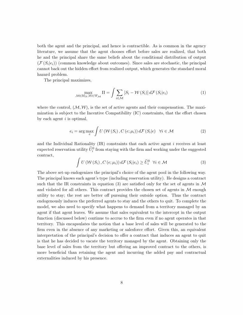
both the agent and the principal, and hence is contractible. As is common in the agencyliterature, we assume that the agent chooses effort before sales are realized, that bothhe and the principal share the same beliefs about the conditional distribution of output(F (Si|ei)) (common knowledge about outcomes). Since sales are stochastic, the principalcannot back out the hidden effort from realized output, which generates the standard moralhazard problem.

The principal maximizes,

maxM∈MN ,W∈WM

Π =

ˆ ∑i∈M

[Si −W (Si)] dF (Si|ei) (1)

where the control, (M,W), is the set of active agents and their compensation. The maxi-mization is subject to the Incentive Compatibility (IC) constraints, that the effort chosenby each agent i is optimal,

ei = arg maxe

ˆU (W (Si) , C (e;µi)) dF (Si|e) ∀i ∈M (2)

and the Individual Rationality (IR) constraints that each active agent i receives at leastexpected reservation utility U0

i from staying with the firm and working under the suggestedcontract, ˆ

U (W (Si) , C (e;µi)) dF (Si|ei) ≥ U0i ∀i ∈M (3)

The above set-up endogenizes the principal’s choice of the agent pool in the following way.The principal knows each agent’s type (including reservation utility). He designs a contractsuch that the IR constraints in equation (3) are satisfied only for the set of agents in Mand violated for all others. This contract provides the chosen set of agents inM enoughutility to stay; the rest are better off pursuing their outside option. Thus the contractendogenously induces the preferred agents to stay and the others to quit. To complete themodel, we also need to specify what happens to demand from a territory managed by anagent if that agent leaves. We assume that sales equivalent to the intercept in the outputfunction (discussed below) continue to accrue to the firm even if no agent operates in thatterritory. This encapsulates the notion that a base level of sales will be generated to thefirm even in the absence of any marketing or salesforce effort. Given this, an equivalentinterpretation of the principal’s decision to offer a contract that induces an agent to quitis that he has decided to vacate the territory managed by the agent. Obtaining only thebase level of sales from the territory but offering an improved contract to the others, ismore beneficial than retaining the agent and incurring the added pay and contractualexternalities induced by his presence.

8

Equivalent Bi-level Setup We can reformulate the problem by allowing to principalto choose the optimal contract in a first step, and then solving point wise for the optimalconfiguration for the chosen contract. The program described above is equivalent to thecase where the principal maximizes,

Π = maxW∈WM

ˆ ∑i∈M

[Si −W (Si)] dF (Si|ei)

with,

M =

ˆ ∑i∈M

[Si −WM (Si)] dF (Si|ei)

subject to the IC and IR constraints as before. Contractual extrenalites arise becausesome elements of the contractW (Si) are common across agents, which makes the problemnon-separable across agents. SinceM∈MN is point-wise the optimal sub-salesforce planfor each considered contractW, the solution to this revised problem returns the solution tothe original program. Representing the program this way helps understand our numericalalgorithm for solution more clearly.

3 Application Setting

To illustrate the main forces at work clearly and to operationalize the setup above for ourempirical setting, we now discuss the parametric assumptions we impose. We employ aversion of the well-known Holmstrom and Milgrom (1987) model for two reasons:

1. The model has a closed-form solution that is useful from both an illustrational anda computational point of view.

2. The optimal contracts are linear (salary plus commission) which is empirically rele-vant.

Though linear contracts are used as the illustrational vehicle, the qualitative aspects ofthe setup holds more generally for any multilateral contracting problem with inter-agentexternalities induced by common contractual components. Each agent i is described com-pletely by a tuple hi, ki, di, ri, σi, Uoi . The elements of the tuple will become clear inwhat follows. Sales are assumed to be generated by the following functional,

Si = hi + kiei + σiεi (4)

This functional has been used in the literature (see e.g. Lal and Srinivasan 1992) andinterprets h as the expected sales in the absence of selling effort (i.e. E [Si|ei = 0] = hi) ,

k as the marginal productivity of effort and σ2 as the uncertainty in the sales production

9

process. As is usual, we assume that the firm only observes Si and knows h, k, σ forall agents. The density F (Si|ei) is induced by the density of εi. Under linear contracts,compensation given as αi + βSi.

The agent’s utility function is defined as CARA,

Ui = − exp −riWi (5)

with wealth linear in output, and costs which are quadratic in effort,

Wi = αi + βSi −di2e2i (6)

The agent maximizes expected utility,

E [Ui] = −ˆ

exp

−r(αi + βSi −

di2e2i

)dF (εi)

= − exp

−r(αi + β (hi + kiei)−

di2e2i −

ri2β2σ2i

)(7)

The Certainty Equivalent is,

CEi = αi + β (hi + kiei)−di2e2i −

ri2β2σ2i (8)

which implies that the optimal effort for the agent is,

ei (β) = βkidi

(9)

3.1 The Principal’s Problem

The principal treats agents as exchangeable and cares only about expected profits,

E [Π] = E[∑N

i=1 (Si − βSi − αi)]

(10)

which is maximized subject to,

IC : ei (β) =βkidi

IR : CEi ≥ Uoi (11)

10

In the above, U0i is the certainty equivalent of the outside option utility. The problem can

be simplified by first incorporating the IC constraint,

E [Π] =N∑i=1

(E (Si)− βE (Si)− αi)

=

N∑i=1

(1− β) (hi + kiei (β))− αi (12)

Further if the IR constraint is binding we have,

αi (β) = Uoi −[β (hi + kiei)−

di2e2i −

ri2β2σ2i

](13)

and substituting in we have,

E [Π] =N∑i=1

[(1− β) (hi + kiei (β))− Uoi +

β (hi + kiei (β))− di

2 ei (β)2 − ri2 β

2σ2i

]=

N∑i=1

[hi + kiei (β)− Uoi −

di2ei (β)2 − ri

2β2σ2i

](14)

Differentiating with respect to β we get,

∂E [Π]

∂β=

N∑i=1

kie′i (β)− die′i (β)− riβσ2i (15)

where,

e′i (β) =∂ei (β)

∂β=kidi

(16)

which gives the optimal uniform commission,

β =1

1 + γ(17)

where, γ,

γ =

∑Ni=1 riσ

2i∑N

i=1k2idi

is an aggregate measure of the distribution of types within the firm. The salary, αi canbe obtained by substitution. Equation (17) encapsulates the effect of each agent type onthe contract: the optimal αi, β depends on the distribution of characteristics of the entire

11

agent pool. Equation (17) demonstrates the contractual externality implied by homogene-ity restrictions: when an agent joins or leaves the salesforce, he affects everyone else bychanging the optimal β. Equation (17) also helps us build intuition about how the distri-bution of types in the firms shifts the common commission rate. Holding everything elsefixed, an increase in the level of risk aversion in the salesforce increases γ, which reduces thecommission rate as expected. As normalized productivity, k

2idi, increases in the salesforce, γ

falls, and optimal commissions increase as expected. Both are intuitive. An assessment ofthe net effect on commissions as both risk aversion and normalized productivities changeis more difficult, as it depends on the extent of affiliation between these parameters in thesalesforce (e.g., whether more risk-averse agents are more productive or less).

To see how the profit function depends overall on agent’s types, we can write equation(14) evaluated at the optimal commission β as,

E [Π (β)] =N∑i=1

(hi − Uoi ) +β

2

(N∑i=1

k2idi

)(18)

Noting that di is the agent’s cost of effort, we can think of 1/di as a measure of theagent’s efficiency − those with higher 1/di expend the same effort at lesser cost. Equation(18) can be interpreted as decomposing the firm’s total profits at the optimally chosenincentive level into two components. The first comprises the total baseline revenue fromeach agent when each is employed, but expending zero effort, (hi−U0

i ). The second is theoptimal commission rate times a weighted average of each agent’s efficiency (1/di), wherethe weights correspond to each agent’s productivity (k2i ). The first part is the insurancecomponent of the incentive scheme, while the second part reflects incentives. Equation(18) also shows that profits are separable across agents except for the choice of β. In theabsence of endogenizing β, the decision to retain an agent i in the pool has no bearing onthe decision to retain another.

Substituting for the optimal β from equation (17), we can write the total payoff to theprincipal with optimally chosen incentives as,

E [Π] =N∑i=1

(hi − Uoi ) +1

2

(∑Ni=1

k2idi

)2(∑Ni=1

k2idi

+∑N

i=1 riσ2i

) (19)

Equation (19) shows that at the optimal β∗, the payoff across agents is no longer separableacross types. Equation (19) defines the firm’s optimization problem over the N agent typesgiven optimal choice of incentives for each sub-configuration.

To build intuition, suppose the firm has the option of retaining three agents with low,medium and high risk aversion. If forced to retain all three on the payroll on a salary +commission scheme, the firm is not able to have a very high-powered incentive scheme with

12

a high commission rate because the high risk-averse agent has to be provided significantinsurance. Firing the high risk averse agent will allow the firm to optimally charge ahigher commission rate to the remaining two agents. Depending on the productivity andcost parameters of the three agents, we can construct examples where the payoffs to thefirm with two agents and the high commission are higher than with three agents and thelower commission.

A Simple 3-Agent Example

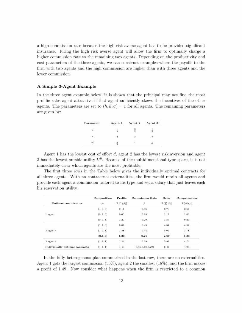
In the three agent example below, it is shown that the principal may not find the mostprolific sales agent attractive if that agent sufficiently skews the incentives of the otheragents. The parameters are set to (h, k, σ) = 1 for all agents. The remaining parametersare given by:

Parameter Agent 1 Agent 2 Agent 3

d 15

32

12

r 4 3 5

U0 94

1 0

Agent 1 has the lowest cost of effort d, agent 2 has the lowest risk aversion and agent3 has the lowest outside utility U0. Because of the multidimensional type space, it is notimmediately clear which agents are the most profitable.

The first three rows in the Table below gives the individually optimal contracts forall three agents. With no contractual externalities, the firm would retain all agents andprovide each agent a commission tailored to his type and set a salary that just leaves eachhis reservation utility.

Composition Profits Commission Rate Sales Compensation

Uniform commissions M E [Π (β)] β E [∑Si] E [WM]

1 agent

(1, 0, 0) 0.14 0.56 3.78 3.64

(0, 1, 0) 0.06 0.18 1.12 1.06

(0, 0, 1) 1.29 0.29 1.57 0.29

2 agents

(1, 1, 0) 0.02 0.45 4.54 4.52

(1, 0, 1) 1.28 0.44 5.06 3.78

(0,1,1) 1.33 0.25 2.67 1.33

3 agents (1, 1, 1) 1.24 0.39 5.99 4.74

Individually optimal contracts (1, 1, 1) 1.49 (0.56,0.18,0.29) 6.47 4.99

In the fully heterogenous plan summarized in the last row, there are no externalities.Agent 1 gets the largest commission (56%), agent 2 the smallest (18%), and the firm makesa profit of 1.49. Now consider what happens when the firm is restricted to a common

13

commission, but individual salaries for each agent. The results are given in the upperrows. Solving for each configuration, we find that the firm would optimally drop agent 1from the pool (expected payoff of 1.33 with an optimal common commission rate to agents2 and 3 of 25%). Including agent 1 in the composition requires the firm to set a highercommission rate (39%), which is too high for the other agents, reducing the firm’s payoffsto 1.24.

Looking at the first two rows of the two agent compositions, agent 1’s presence in thepool is seen to exert skew the incentives of agent 2 and 3 away from their individually opti-mal commissions. If only agent 1 is retained, he would be paid a high-powered commissionrate of 56%, while agents 1 and 2 prefer commissions of only 18% and 29% respectively. Inthis example, the firm is better off dropping the high-powered sales-agent from the pool.Without agent 1, the firm can set an intermediate level of commissions (25%) that provides2 and 3 better incentives. For a more dramatic effect, consider agent 1 and 2 individually.At the heterogenous contracts at individual commissions 56% and 18%, they bring in prof-its of 0.20. Under a uniform commission commission of 45%, the profit is reduced to 0.02,as agent 1 gets underpowered incentives and agent 2 gets overpowered incentives.

The firm makes lower sales with only agents 2 and 3 than with 3 agents (2.67 versus5.99), but compensation payout is also lower, and the net effect is a higher profit. Bychanging parameters, we can generate other examples where the low-commission agent isdropped from the pool in order to set high-powered incentives for the remaining agents,which is the mirror-image to this setting. The example below also illustrates the compli-cation induced by multidimensional types: the desirability of an agent cannot be orderedon any one dimension by a simple cut-off rule.

Note that the profits under the optimal uniform commission plan (1.33) come close tothat of the individual optimal plan (1.49), despite the restriction to common commissionsand the heterogeneity in individually optimal commissions. The example illustrates howcareful choice of composition can compensate for the reduced incentives implied by thecommon contract terms, a point that also shows up in our empirical application below.

The simple example shows how composition and compensation interact in influencingfirm profits. While the example has only three agents, it provides a glimpse into theworkings of this interaction, and in particular shows that commonly used performancemeasures such as sales (or even profit contribution) may not be useful in determining whichagents should stay. Indeed, in the above example, agent 1 had the highest productivity interms of sales (3.78 vs. 1.12 and 1.57 for agents 2 and 3) and the second highest profitcontribution (.14 vs .06 and 1.29 for agents 2 and 3). However, keeping the agent in thepool distorted the incentives to the others. We conjecture that similar patterns apply moregenerally in real world sales-forces. To examine this conjecture we use data from a realsalesforce below. Before doing so, we introduce our algorithm to compute the optimalsalesforce composition.

14

4 The Solution Algorithm

The simple example presented above used a complete enumeration of possible salesforcecompositions to examine profitability. Real-world sales-forces often numbers in the hun-dreds or thousands, and this approach is not practical. The joint determination of thecomposition and compensation is a non-standard mixed-integer program. Nevertheless,the decomposition of the problem into two parts we outlined above converts it into a formthat can be solved by standard methods. We solve the joint problem by an inner-outer loopprocedure. In the inner loop, we solve for the optimal composition for any compensation.In the outer loop, we search over compensations. Despite the combinatorial nature of thecomposition problem, we show how to concentrate out the exact optimal composition con-ditional on the contracts in a convenient form. The complexity of the resulting programis linear in N and the search over compensations is a standard optimization problem.

The key to our algorithm is to note that all the externalities are channeled throughthe contracts. Holding the contract fixed, the individual profitability of any agent isindependent of the composition itself. The principal’s question of whether to keep anagent or not at given contract therefore depends only on whether the agent is profitableand not on the composition itself. Hence, conditioning on the contract helps address thecombinatorial explosion.

Equation (17) gives the optimal common commission β for any considered compositionprofile. Given β one can invert out the firm optimal salaries from the IR constraint agent-by-agent,

α(β) : CEi(αi, β) = U0i (20)

where we note that the optimal salaries α(β) are continuous in β. The optimal contractsare now summarized by β. Define agent i′s profit contribution at contract β,

πi(β) = E[Si(β)− (αi(β)− βSi)] for all i ∈M

We then show that at the optimum, the profit contribution of any included agent is positive.

Proposition 1 At the optimal composition-compensations (M∗, β(M∗))

1. πi(β(M∗)) ≥ 0 for all i ∈M∗

2. πi(β(M∗)) < 0 for all i ∈ (1, .., N)\M∗

Proof. For the first part, suppose not, and that πi′(β(M∗)) < 0 for some agent i′ ∈ M∗.Then the firm could fire agent i′ and hold the compensation W(β(M∗)) fixed for the re-maining agents in M∗\i′. Since none of the remaining agents face different incentives,their profit contributions stay constant and net profits would improve. But that con-

15

tradicts the optimality of the composition-compensation (M∗, β(M∗)). It follows thatπi(β(M∗)) ≥ 0 for all i ∈M∗. Part 2 follows by analogous logic.

The intuition is simple: if an excluded agent can be profitably employed without chang-ing the incentives of the other agents, than he for sure can be profitably employed at acommission optimized for the composition including him. If so, he belongs to the optimalcomposition and we have a contradiction. Given positivity of conditional profits as above,we can then construct a conditional value function that concentrates out the compositionproblem conditional on β:

π(β) =∑

i∈(1,..N)

1πi≥0πi(β). (21)

The concentrated value function sums the profit contributions of the agents that are re-tained in the optimal composition conditional on β. Since the composition problem condi-tional on β involves integer optimization, one may suspect the conditional value functionis discontinuous, precluding a smooth search over β. We now prove the following usefulproperty of the conditional value function:

Proposition 2 The conditional value function π(β) is continuous in β.

Proof. Both the expectation of the sales process in Equation (4) and the concentratedsalaries in Equation (20) are continuous functions of β, so it follows that the πi(β) iscontinuous in β for all i ∈ (1, .., N). The profit contribution of any agent i to the conditionalvalue function in Equation (21) is the upper envelope of two continuous functions of β,that is max0,E[Si(β)(1−β)−αi(β)], which is itself continuous. Finally, the conditionalvalue function in Equation (21) sums the non-negative profit contributions of all agentsi ∈ (1, ..N) for any β, and is itself the sum of continuous functions, and therefore alsocontinuous.

Note that the continuity property places no restrictions on the underlying distributionsof agents parameters, which facilitates empirical work.

4.1 Algorithm

The results above give us the solution algorithm:

1. For a given β, calculate πi(β) for all i ∈ (1, .., N).

2. Search the conditional value function (21) over [0, 1] for the optimal β∗.

At β∗, the optimal composition is i : πi(β) > 0, i ∈ (1, .., N). The algorithm reduces thejoint problem to a search of a continuous function over a compact set, which is a standardoptimization problem. Importantly, the algorithm is linear in N even though the space ofcompositions increases exponentially. Utilizing this characterization enables us to reduce

16

the problem to a unidimensional search over β ∈ [0, 1], rather than a combinatorial searchover the the space of 2N compositions. For N moderately large, this approach can yielda significant improvement in terms of computational time. More importantly, since theproblem is smooth and continuous in β, the optimization approach facilitates comparativestatics and hence insights into properties of the solution. Some numerical examples of thealgorithm for various sizes of N is given in the appendix.

5 Empirical Application

Our data come from the direct selling arm of the sales-force division of a large contactlens manufacturer in the US (we cannot reveal the name of the manufacturer due to con-fidentiality reasons). These data were used in Misra and Nair (2001), and some of thedescription in this section partially borrows from that paper. Contact lenses are primar-ily sold via prescriptions to consumers from certified physicians. Importantly, industryobservers and casual empiricism suggests that there is little or no seasonality in the under-lying demand for the product. The manufacturer employs a direct salesforce in the U.S.to advertise and sell its product to physicians (also referred to as “clients”), who are thesource of demand origination. The data consist of records of direct orders made from eachdoctor’s office via a online ordering system, and have the advantage of tracking the timingand origin of sales precisely. Agents are assigned their own, non-overlapping, geographicterritories, and are paid according to a nonlinear period-dependent compensation schedule.Pricing issues play an insignificant role for output since the salesperson has no control overthe pricing decision and price levels remained fairly stable during the period for which wehave data. The compensation schedule for the agents involves salaries, quotas and ceilings.Commissions are earned on any sales exceeding quota and below the ceiling. The salary ispaid monthly, and the commission, if any, is paid out at the end of the quarter. The saleson which the output-based compensation is earned are reset every quarter. Additionally,the quota may be updated at end of every quarter depending on the agent’s performance(“ratcheting”). Our data includes the history of compensation profiles and payments forevery sales-agent, and monthly sales at the client-level for each of these sales-agents for aperiod of about 3 years (38 months).

The firm in question has over 15,000 SKU-s (Stock Keeping Units) of the product.The product portfolio reflects the large diversity in patient profiles (e.g. age, incidenceof astigmatism, nearsightedness, farsightedness etc.), patient needs (e.g. daily, disposableetc.) and contact lens characteristics (e.g. hydrogel, silicone-hydrogel etc.). The productportfolio of the firm features new product introductions and line extensions reflecting thelarge investments in R&D and testing in the industry. The role of the sales-agent ispartly informative, by providing the doctor with updated information about new productsavailable in the product-line, and by suggesting SKU-s that would best match the needs ofthe patient profiles currently faced by the doctor. The sales-agent also plays a persuasive

17

role by showcasing the quality of the firm’s SKU-s relative to that of competitors. Whileagent’s frequency of visiting doctors is monitored by the firm, the extent to which he“promotes” the product once inside the doctor’s office cannot be monitored or contractedupon. In addition, while visits can be tracked, whether a face-to-face interaction with adoctor occurs during a visit in within the agent’s control (e.g., an unmotivated agent maysimply “punch in” with the receptionist, which counts as a visit, but is low on effort).3

Misra and Nair (2011) used these data to estimate the underlying parameters of theagent’s preferences and environments using a structural dynamic model of forward-lookingagents. For our simulations, we use some parameters from that paper, while some are cali-brated. We provide a short overview of the model and estimation below, noting differencesfrom their analysis in passing.

5.1 The Model for Sales-Agents

The compensation scheme involves a salary, αt, paid in month t, as well as a commissionon sales, βt. The sales on which the commission is accrued is reset every N months.The commission βt is earned when total sales over the sales-cycle, Qt, exceeds a quota,at, and falls below a ceiling bt. No commissions are earned beyond bt. Let It denote themonths since the beginning of the sales-cycle, and let qt denote the agent’s sales in month t.Further, let χt be an indicator for whether the agent stays with the firm. χt = 0 indicatesthe agent has left the focal company and is pursuing his outside option. Assume that oncethe agent leaves the firm, he cannot be hired back (i.e. χt = 0 is an absorbing state). Thetotal sales, Qt, the current quota, at, the months since the beginning of the cycle It, andhis employment status χt are the state variables for the agent’s problem. We collect thesein a vector st = Qt, at, It, χt, and collect the observed parameters of his compensationscheme in a vector Ψ = α, β . We will use the data in combination with a model of agentbehavior to back out the parameters indexing agent’s types. The results in this paper areobtained taking these parameters as given.

The index i for agent is suppressed in what follows below. At the beginning of eachperiod, we assume the agent observes his state, and chooses to exert effort et. Based on hiseffort, sales qt are realized at the end of the period. Sales qt is assumed to be a stochastic,increasing function of effort, e and a demand shock, εt, qt = q (εt, e) . The agent’s utility isderived from his compensation, which is determined by the incentive scheme. We write theagent’s monthly wealth from the firm as, Wt = W (st, et, εt;µ,Ψ) and the cost function asde2t2 , where d is to be estimated. We assume that agents are risk-averse, and that conditionalon χt = 1, their per-period utility function is,

ut = u (Qt, at, It, χt = 1) = E [Wt]− r × var [Wt]−de2t2

(22)

3The firm does not believe that sales-visits are the right measure of effort. Even though sales-calls areobserved, the firm specifies compensation based on sales, not calls.

18

Here, r is a parameter indexing the agent’s risk aversion, and the expectation and vari-ance of wealth is taken with respect to the demand shocks, εt. In the case of a salary+ piece-rate of the type considered before, equation (22) collapses to exactly the formdenoted in equation (8) for the certainty equivalent. We can thus interpret equation (22)as the nonlinear-contract analogue to the certainty equivalent of the agent under a linearcommission. The payoff from leaving the focal firm and pursuing the outside option isnormalized to U0,

ut = u (Qt, at, It, χt = 0) = U0 (23)

In this model, sales are assumed to be generated as a function of the agent’s effort, whichis choose by the agent maximizing his present discounted payoffs subject to the transitionof the state variables. The first state variable, total sales, is augmented by the realizedsales each month, except at the end of the quarter, when the agent begins with a freshsales schedule, i.e.,

Qt+1 =

Qt + qt if It < N

0 if It = N(24)

For the second state variable, quota, we estimate a semi-parametric transition functionthat relates the updated quota to the current quota and the performance of the agentrelative to that quota in the current quarter,

at+1 =

at if It < N∑K

k=1 θkΓ (at, Qt + qt) + vt+1 if It = N(25)

In above, the new quota is allowed to depend flexibly on at and Qt + qt, via a Korderpolynomial basis indexed by parameters, θk to capture in a reduced-form way, the man-ager’s policy for updating agent’s quotas. The term vt+1 is an i.i.d. random variate whichis unobserved by the agent in month t. The distribution of vt+1 is denoted Gv (.) , andwill be estimated from the data. Finally, the transition of the third state variable, monthssince the beginning of the quarter, is deterministic,

It+1 =

It + 1 if It < N

1 if It = N(26)

Finally, the agent’s employment status in (t+ 1), depends on whether he decides to leavethe firm in period t. Given the above state-transitions, we can write the agent’s problemas choosing effort to maximize the present-discounted value of utility each period, wherefuture utilities are discounted by the factor, ρ. We collect all the parameters describingthe agent’s preferences and transitions in a vector Ω = µ, d, r,Gε (.) ,Gv (.) , θk,k=1,..,K.In month It < N , the agent’s present-discounted utility under the optimal effort policycan be represented by a value function that satisfies the following Bellman equation (see

19

Misra and Nair 2011),

V (Qt, at, It, χt; Ω,Ψ) =

maxχt+1∈(0,1),e>0

u (Qt, at, It, χt, e; Ω,Ψ)

+ρ´ε V (Qt+1 = Q (Qt, q (εt, e)) , at+1 = at, It + 1, χt+1; Ω,Ψ) f (εt) dεt

(27)

Similarly, the Bellman equation determining effort in the last period of the sales-cycle is,

V (Qt, at, N, χt; Ω,Ψ) =

maxχt+1∈(0,1),e>0

u (Qt, at, N, χt, e; Ω,Ψ)

+ρ´v

´ε V (Qt+1 = 0, at+1 = a (Qt, q (εt, e) , at, vt+1) , 1, χt+1; Ω,Ψ)

× f (εt)φ (vt+1) dεtdvt+1

(28)

Conditional on staying with the firm, the optimal effort in period t, et = e (st; Ω,Ψ)

maximizes the value function,

e (st; Ω,Ψ) = arg maxe>0

V (st; Ω,Ψ) (29)

The agent stays with the firm if the value from employment is positive, i.e.,

χt+1 = 1 if maxe>0V (st; Ω,Ψ) > 0

This completes the specification of the model specifying the agent’s behavior under theplan that generated the data. Given this set-up, the structural parameters describing anagent Ω, are estimated in two steps.

Estimation

First, we recognize that once effort, et is estimated, we can treat hidden actions as known.The theory implies st is the state vector for the agent’s optimal dynamic effort choice. Wecan use the theory, combined with dynamic programming to solve for the optimal policyfunction e∗ (st; Ω), given a guess of the parameters Ω. Because et is known, we can then useet = e∗ (st; Ω) as a second-stage estimating equation to recover Ω. Misra and Nair (2011)implement this approach agent-by-agent to recover Ω for each agent separately. Theyexploit panel-data available at the client-level for each agent to avoid imposing cross-agentrestrictions, thereby obtaining a semi-parametric distribution of the types in the firm.

The question remains how the effort policy, et = e (st) can be obtained? The intuition

20

used in Misra and Nair is to exploit the nonlinearity of the contract combined with paneldata for identification. The nonlinearity implies the history of output within a compensa-tion horizon is relevant for the current effort decision, because it affects the shadow cost ofworking today. Thus, effort is time varying, and dynamically adjusted. The relationshipbetween current output and history is observed in the data. This relationship will pin downhidden effort. Intuitively, the path of output within the compensation cycle is informativeof effort. We refer the reader to that paper for further details of estimation and identifi-cation.4 For the counterfactuals in this paper, we need estimates of

h, k, d, r, U0,Gε (.)

.

Here, we assume that Gε (.) ∼ N(0, σ2

). So, we need θ ≡

h, k, d, r, U0, σ

. We use the

same parameters from Misra and Nair for these, estimating σ from imposing the normalityassumption of the recovered demand-side errors from the model. The parameter, k, isnot estimated in Misra-Nair. Here, we exploit additional data not used in that paper onthe number of calls made by each agent i to a client j in month t, which we denote as,kijt. We observe kijt and obtain a rough approximation to ki as ki ≈ 1

T

∑t

∑j kijt. The

incorporation of k into the model does not change any of the other parameters estimatedin Misra-Nair, and only changes their interpretation. We use these parameters for all thesimulations reported below.

6 Results

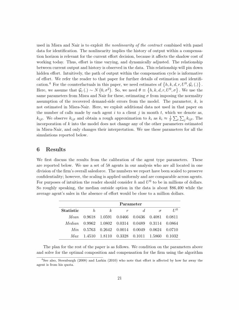
We first discuss the results from the calibration of the agent type parameters. Theseare reported below. We use a set of 58 agents in our analysis who are all located in onedivision of the firm’s overall salesforce. The numbers we report have been scaled to preserveconfidentiality; however, the scaling is applied uniformly and are comparable across agents.For purposes of intuition the reader should consider h and U0 to be in millions of dollars.So roughly speaking, the median outside option in the data is about $86,400 while theaverage agent’s sales in the absence of effort would be close to a million dollars.

ParameterStatistic h k r d σ U0

Mean 0.9618 1.0591 0.0466 0.0436 0.4081 0.0811

Median 0.9962 1.0802 0.0314 0.0489 0.3114 0.0864

Min 0.5763 0.2642 0.0014 0.0049 0.0624 0.0710

Max 1.4510 1.8110 0.3328 0.1011 1.5860 0.1032

The plan for the rest of the paper is as follows. We condition on the parameters aboveand solve for the optimal composition and compensation for the firm using the algorithm

4See also, Steenburgh (2008) and Larkin (2010) who note that effort is affected by how far away theagent is from his quota.

21

described previously. We then discuss these below, simulating two different scenarios.First, we simulate the fully heterogeneous plan where each agent receives a compensationplan (salary + commission) tailored specifically for him or her. We also simulate thepartially homogenous contract where the commission rate is common across agents butthe salaries may vary across individuals. In all the results presented below, we assumethat when an agent is excluded from the salesforce, the territory provides revenues equalto τh with τ = 0.95, and h is the intercept in the output equation. This assumption reflectsthe fact that even if a territory is vacated, sales would still accrue on account of the brandor because the firm might use some other (less efficient) selling approach like advertising.We also explored alternative assumptions (e.g. τ = 0 and τ = 1); these results are availablefrom the authors upon request. Qualitatively, the results obtained were similar to thosepresented below. Below we organize our discussion by presenting details of the optimalcomposition chosen by the firm under these plans, and then present details of effort, salesand profits.

6.1 Composition

We start with the fully heterogeneous plan as a benchmark. We find all agents havepositive profit contributions when plans can be fully tailored to their types. Consequently,the optimal configuration under the fully heterogeneous plan is to retain all agents (the“status quo”). This is not surprising as noted in our 3-agent simulation previously.

Simulating the partially heterogeneous compensation plans, we find the optimal com-position in this salesforce would involve letting go of six salespeople. It is interesting toinvestigate the characteristics of the agents who are dropped and to relate it to that of theagent pool as a whole. In Figure (1) we plot the joint distribution of the primitive agenttypes

h, k, d, r, U0, σ

for all agents at the firm. The marginal densities of each parameter

across agents is presented across the diagonal. Each point in the various two-way plotsalong the off-diagonals is an agent, and each two-way shows a scatter-plot of a particularpair of agents types, across the agent pool. For instance, plot [4,1] in Figure (1) shows ascatter-plot of risk aversion (r) versus the cost of effort (d) across all agents in the pool.Plot [1,4] is symmetric and shows a scatter-plot of cost of effort (d) versus risk aversion(r). The six agents who are not included in the optimal composition are represented bynon-solid symbols, highlighted in red. For instance, we see that one of the dropped agents,represented as an “o”, has a high risk aversion (1st row), an average level of sales-territoryvariance (2nd row), an average level of productivity (3rd row), a low cost of effort (4th row),a low outside option (5th row), and a lower than average base level of sales (last row). Thisagent has a low cost of effort. However, his high risk aversion, his lower outside option,as well as his fit relative to the distribution of these characteristics across the rest of theagents, implies he is not included in the preferred composition. Figure (1) illustrates theimportance of multidimensional heterogeneity in the composition-compensation tradeoff

22

facing the principal, and emphasizes the importance of allowing for rich heterogeneity inempirical incentive settings.

In Figure 2, we plot the location of these salespeople on the empirical marginal densitiesof the profitability and sales across sales-agents. What is clear from Figure 2 is that there isno a priori predictable pattern in the location of these agents. In some cases, the agents lieat the tail end of the densities, though this does not hold generally. Further, the droppedagents are not uniformly at the bottom of the heap in terms of expected sales or profitcontribution under the fully heterogeneous plan. For example, #33, one of the droppedagents, has expected sales of $1.70MM under the fully heterogeneous plan which wouldplace him/her in the top decile of agents in terms of sales. In addition, he/she is also inthe top decile across agents in terms of profitability. However, in his/her case the varianceof sales is the highest in the firm, and this creates a large distortion in the contract viathe effect it induced on the optimal commission rate (β). No including this agent allowsthe firm to improve the contract terms of other agents thereby increasing profits. Otheragents are similarly not included on account of some other externality that impacted thecompensation contract.

Figure 1 and 2 accentuates the difficulties of ranking agents as desirable or not on thebasis of a single type-based metric and the need for a theory of value to assess sales-agents.

6.2 Compensation

We now discuss the optimal compensation implied for the firm under the optimal compo-sition. We compare the fully heterogeneous plan to the partially homogenous plans withand without optimizing composition. Figure (3) plots the density of optimal commissionrates under the fully heterogeneous plan along with those for the partially homogenousplans. The solid vertical lines are drawn at the common commission rate for the homoge-nous plans, with the blue vertical line corresponding to optimizing composition and theblack corresponding to not optimizing composition. Looking at Figure (3), we see that thecommission rates vary significantly across the sales-agents under the fully heterogeneousplans, going as high as 2.5% for some agents (median commission of about 1.2%). Underthe partially homogenous plans, the optimal commission rates are lower. Interestingly, theability to fine tune composition has significant bite in this setting. In particular, whenconstrained to not fine tune the salesforce, the firm sets an optimal common commissionof about 0.5%. When it can also fine tune the salesforce, the firm optimally sets a highercommission rate of about 0.9%. When the firm is constrained by the compensation struc-ture, the extreme agents (eliminated in the optimal composition) exert an externality thatbrings the overall commission rate down. By eliminating the “bad” agents, the firm is ableto increase incentives. To what extent does does this improve effort, sales and profitability?We discuss this next.

23

Figure 1: Joint Distribution of Characteristics of Agents who are Retained and Droppedfrom Firm under Partially Homogenous Plans

|||| || ||| | | ||||| || |||||||| | ||| | | ||||| || | ||| | ||||| || | |||| | |

r

500 1000 1500 0.02 0.06 0.10 0.6 1.0 1.4

0.00

0.10

0.20

0.30

500

1000

1500

|| | || || | ||| |||| || || || || | |||| |||| || ||| |||| ||||| | | ||| ||| | |||

s

|||||| | || ||| ||| || || |||| | |||| | ||| ||| |||| | |||| || | |||| ||| | || |

k

0.5

1.0

1.5

0.02

0.06

0.10

| ||| ||||| | || || || | ||| || |||||| | |||| ||| || | ||| |||| | || || | ||| |||

d

| ||| ||| || ||| ||| | | ||| |||| ||||| | || | || | || || |||| || |||| || | | || ||

u00.070

0.085

0.100

0.00 0.10 0.20 0.30

0.6

1.0

1.4

0.5 1.0 1.5 0.070 0.085 0.100

|| |||| | ||||| | || ||| | || ||| || ||| | |||||| | ||| ||| ||| |||| |||| || | |

h

24

Figure 2: Profitability and Sales of Eliminated Sales Agents

-0.5 0.0 0.5 1.0 1.5

0.0

0.5

1.0

1.5

Contribution Under Status Quo

0.0 0.5 1.0 1.5 2.0 2.5

0.0

0.5

1.0

1.5

E(Sales) Under Status Quo

Composition →Compensation ↓ Status Quo OptimalFully Heterogeneous $60.56MM $60.56MMPartially Homogenous $55.78MM $59.14MM

Table 1: Profits under Fully and Partially Heterogenous Plans

6.3 Effort and Outcomes

The profits for the firm under the fully heterogeneous plan are estimated to be around$60.56MM. We decompose profits with and without homogenous plans, with and with-out optimizing composition. As noted above, in our data all agents have positive profitcontributions and consequently, the optimal configuration is identical to the status quofor compensation plans that are fully heterogeneous. Consequently profits for the fullyheterogeneous plan under the optimal configuration and the status quo are identical. Thisis depicted in the first row of Table (1).

In contrast to the fully heterogeneous compensation structure, there is a significantdifference in profit levels when compensation plans cannot be customized. Looking at theabove table, partially homogenous plans with the ability to fine-tune composition comevery close to the fully-heterogeneous plan in terms of profitability ($59.14MM compared to$60.56MM). But partially homogenous plans without the ability to fine-tune the salesforce

25

Figure 3: Optimal Commission Rates Under Fully Heterogeneous, Fully Homogenous andPartially Homogenous Plans

0.000 0.005 0.010 0.015 0.020 0.025

020

4060

80

Commission Rate

f(com

mis

sion

rate

)

Status Quo Full-Het PlanOptimal Partial-Het PlanStatus Quo Partial-Het Plan

26

causes a distortion in incentives, and result in a profit shortfall of $3.36MM, bringing thetotal profits down to $55.78MM.

To decompose the source of profitability differences across the different scenarios, inFigures 4a and 4b we depict the empirical CDF of effort and sales under the three scenarios.The “status-quo” plan is the one that keeps the same composition as currently, but changescompensation. Both the sales and effort distributions under the fully heterogeneous planfall to the right of the partially heterogeneous plans. However, Kolmogorv-Smirnoff testsshow that the distribution of sales and effort under the composition and compensationoptimized scenario is not statistically different from that under the fully heterogeneousplan. This is striking, since it suggests that by simply altering composition in conjunctionwith compensation a firm can reap large dividends in motivating effort, even under theconstraints of partial homogeneity in contractual terms. This is also why the overallprofits under the optimal composition with common commissions is so close to that underheterogeneous plans.

We now assess the extent to which profits at the individual sales-agent level under thepartially homogenous plan combined with the ability to choose the composition of agents,approximates the profitability under the fully heterogeneous plan (the baseline or best-casescenario). In Figure 6, we plot the profitability (revenues − payout) of each agent underthe fully heterogeneous plan on the x-axis, and the profitability under the partially ho-mogenous plan with and without the ability to optimize composition on the y-axis. Soliddots represent profits when optimizing composition, while empty dots represent profitsholding composition fixed at the status quo. Each point represents an agent. Numbersare in $MM-s. Looking at Figure 6, we see the ability to choose composition is important.In particular, the profitability at the agent-level when constrained to partially homoge-nous contracts and not optimizing composition lies much below the profitability under asituation where contracts can be fully tailored to each agent’s type. But, the ability tochoose agents seems to be able to mitigate the loss in incentives implied by the constraintto homogeneity. The profitability under the composition-optimized, partially homogenouscontracts come very close to that under fully tailored contracts.

We think this is an important take away. In the real-world, firms can choose bothagents and incentives, and not incentives alone. Firms do face constraints when settingincentives. But, our results suggest that the profit losses associated with these constraintsare lower when firms are also able to choose the type-space of the agents concomitant withincentives.

Mechanism

The question remains what is the mechanism that enables the firm to come close to thefully heterogeneous plan when it optimizes the composition of its agents? The intuitionis straightforward. When constrained to set a homogenous plan, a firm can do much

27

Figure4:

EmpiricalCDF

ofIm

pliedEffo

rtan

dSa

lesUnd

erDifferentCou

nterfactua

lCom

pensationan

dCom

position

Profiles

(a)EmpiricalC

DFof

Effo

rtProfiles

(b)EmpiricalC

DFof

Exp

ectedSa

les

28

better if the agents it has to incentivize are more homogenous. Consider an extreme casewhere the firm could find as many agents of any type for filling its positions (no searchcosts for labor). Then, the firm would first pick the agent from who it could obtain thehighest profit (output − payout) under the fully tailored heterogenous contract. It wouldthen fill the N available positions with N replications of that agent. Then, the uniformcommission it charges for the salesforce as a whole will be optimal for every agent in thefirm. In this sense, an increase in heterogeneity has two roles for a firm constrained touniform contracts. On the one hand, it increases the chance that high quality agents arein the firm (a positive). But on the other hand, it also increases the level of contractualexternalities (a negative). The optimal composition has to balances these competing forces.

To see this more formally, consider a firm that has demand for two agents, which itcan fill with A or B type agents. Let Θ index type and suppose typeA-s generate moreprofit than B-s when employed at their individually optimal contracts:

ΘA 6= ΘB but E [π (A)] > E [π (B)]

Then, all things held equal, the firm would prefer composition A,A over B,B,

E [π (A,A)] > E [π (B,B)]

Now suppose that types are such that A-s and B-s generate the same profit when employedat their individually optimal contracts,

ΘA 6= ΘB but E [π (A)] = E [π (B)]

Then, even though individual profits are same, the firm would prefer to have the compo-sition A,A or B,B over A,B, because composition A,B generates contractualexternalities,

E [π (A,A)] = E [π (B,B)] > E [π (A,B)]

It is in this sense that the firm has a preference for heterogeneity reduction. Optimalcontracting requires the principal to satisfy both incentive rationality and incentive com-patibility constraints for its chosen agents. Allowing for agent-specific salaries allows thefirm the satisfy incentive rationality for the agents it wants to retain. But the constraintto a common commission implies that incentive compatibility becomes harder to satisfywhen the agent pool becomes more heterogeneous. Hence, a firm that can also choose thepool prefers one that is relatively more homogenous, ceteris paribus.

To empirically assess this intuition, we compute two measures of the spread in the typedistribution of the salesforce under the optimal partially homogenous contacts with andwithout the ability to choose agents. Assessing the dispersion in types is complicated bythe fact that the type-space is multidimensional. We can separately compute the variance-

29

covariance matrix of types in the salesforce under the two scenarios. To compute a singlemetric that summarizes the distribution of types, we define a measure of spread, dM, asthe trace of the variance covariance matrix of agent characteristics,5

dM = tr (ΣM) (30)

We find that dMStatusQuo = 78, 891.6, and dMOptimal = 51, 921.8, where dMStatusQuo is thetrace under the optimally chosen partially homogenous plan while retaining all agents inthe firm, and dMOptimal is the trace under an optimally chosen partially homogenous planwhile jointly optimizing the set of agents retained in the firm. We see that the optimalconfiguration involves about 34.2% reduction in heterogeneity. As another metric, weuse dM = det (ΣM). The determinant can be interpreted as measuring the volume of theparallelepiped spanned by the vectors of agent types. To the extent the volume is lower, thespread in types may roughly be interpreted as lesser. We find that the determinant basedmeasure of spread shows a 80.8% decline when the firm can pick its agents and incentives,relative to picking only incentives. Both illustrate that under the optimal strategy, the firmchooses agents such that the residual pool is more homogeneous. While this is intuitive,what is surprising is that its profits under this restricted situation come so close to whatit would make under fully heterogeneous plans. This can only be assessed empirically.

To assess the intuition visually, we plot in Figure (5), the salaries and commissionsof the entire set of agents when each could be offered his own tailored contract (i.e, thesalary + commissions from the fully heterogeneous case). The green dots in Figure (5)denotes the agents who are retained in the optimal composition while the red dots denotethe agents who are dropped. Also plotted is the convex hull of the salary/commissionpoints. We see that the optimal configuration exhibits a degree of outlier aversion: theagents dropped from the optimal composition are all on the extremes of the distribution.Note at the same time, that being an outlier does not automatically imply an agent isdropped: we see that some agents on the edges are still retained, presumably on accountof their higher abilities or better fit with the rest of the agents.

In an important paper, Raju and Srinivasan (1996) make an analogous point, that al-lowing for heterogeneous quotas in a common commissions setting can closely approximatethe optimal salary + commission based incentive scheme for a heterogeneous salesforcewhen those quotas can themselves reflect agent specific differences. Our point is analo-gous, that a firm constrained to a homogenous slope on its incentive contract can comevery close to the optimum by picking the region of agent-types that it wants to retain.However, the mechanism we suggest is different. Raju and Srinivasan (1996) suggest ad-dressing the problem of providing incentives to a heterogeneous salesforce by allowing foradditional heterogeneity in contract terms. We suggest addressing the problem of settingincentives to a heterogeneous pool of agents by making the salesforce more homogenous.

5The trace of a matrix is the sum of its diagonals.

30

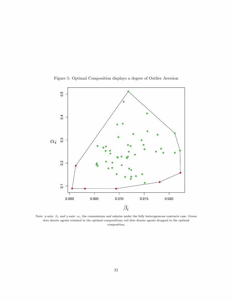
Figure 5: Optimal Composition displays a degree of Outlier Aversion

Note: x-axis: βi, and y-axis: αi, the commissions and salaries under the fully heterogeneous contracts case. Greendots denote agents retained in the optimal compositions; red dots denote agents dropped in the optimal

composition.

31

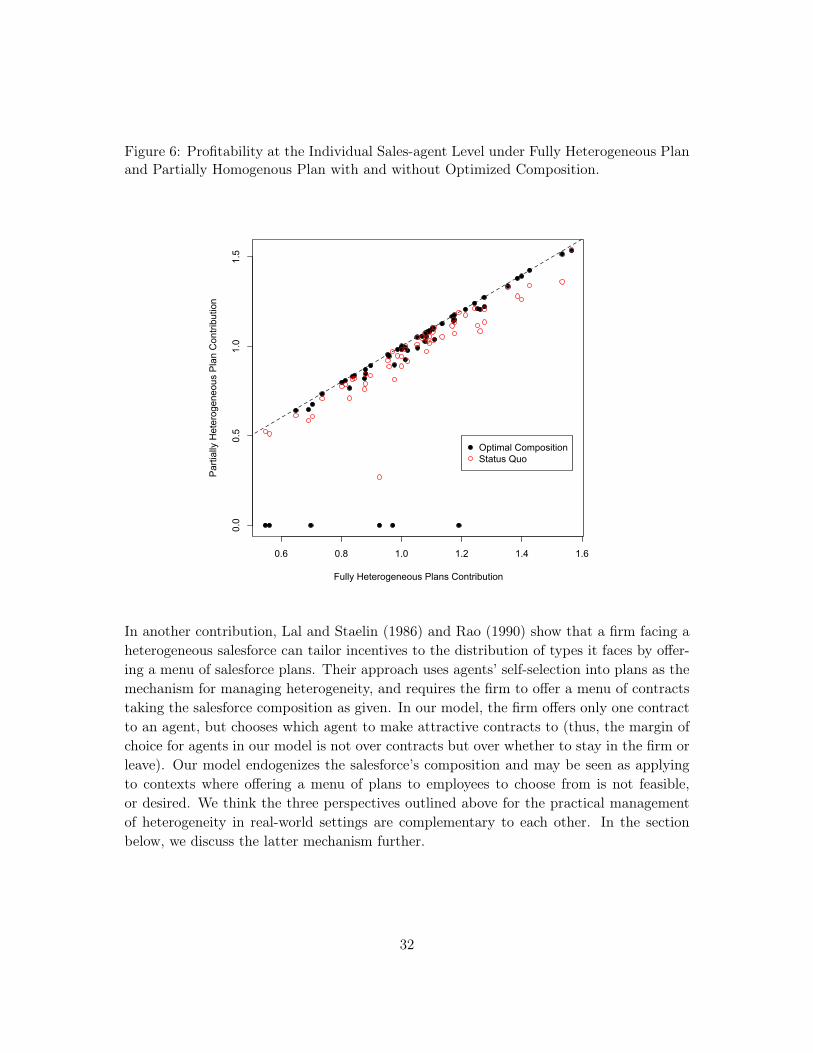
Figure 6: Profitability at the Individual Sales-agent Level under Fully Heterogeneous Planand Partially Homogenous Plan with and without Optimized Composition.

0.6 0.8 1.0 1.2 1.4 1.6

0.0

0.5

1.0

1.5

Fully Heterogeneous Plans Contribution

Par

tially

Het

erog

eneo

us P

lan

Con

tribu

tion

Optimal CompositionStatus Quo

In another contribution, Lal and Staelin (1986) and Rao (1990) show that a firm facing aheterogeneous salesforce can tailor incentives to the distribution of types it faces by offer-ing a menu of salesforce plans. Their approach uses agents’ self-selection into plans as themechanism for managing heterogeneity, and requires the firm to offer a menu of contractstaking the salesforce composition as given. In our model, the firm offers only one contractto an agent, but chooses which agent to make attractive contracts to (thus, the margin ofchoice for agents in our model is not over contracts but over whether to stay in the firm orleave). Our model endogenizes the salesforce’s composition and may be seen as applyingto contexts where offering a menu of plans to employees to choose from is not feasible,or desired. We think the three perspectives outlined above for the practical managementof heterogeneity in real-world settings are complementary to each other. In the sectionbelow, we discuss the latter mechanism further.

32

6.4 Sorting Agents into Divisions

We now discuss whether we can further improve the management of heterogeneity in thefirm by sorting agents into divisions. We consider a salesforce architecture in which thefirm creates |J | divisions, and assigns each agent it retains to one of the |J | divisions. Thedivisions correspond to different compensation profiles. We allow each division to have itsown commission, but require that all agents within a division are given the same commis-sion. Salaries are allowed to be heterogeneous as before. Such architectures are commonlyobserved in the real-world. For instance, salesagents targeting large “key accounts” maybe assigned into a division which offers more incentive pay, while those targeting smallerclients may be in a division that offers more salary than commission. Or alternatively,salesagents targeting urban versus rural clients may be in two different divisions eachwith its own commission scheme. But the observed empirical fact is that commissions areinvariably the same within a division. This architecture reflects that.

For each value of |J | we solve simultaneously for the match between agents and divi-sions and the optimal commissions across divisions, along with the optimal salaries acrossagents given their assignment to a division. Formally, we solve the following modifiedbi-level optimization problem,

maxMj

Π =∑j∈J

ˆ ∑i∈Mj

(Si −WMj (Si)

)dF (Si|ei) , st.,

WMj = arg maxW∈WN

ˆ ∑i∈Mj

(Si −W (Si)) dF (Si|ei) , (IR,IC)

⋃j∈JMj = MN

where the last “adding-up” constraint ensures that a given agent is either assigned to oneof |J | contracts. The incentive compatibility and rationality constraints IR and IC are notwritten out explicitly for brevity. In the final solution to above, the setMj assigns to eachagent i, a number 0, 1, .., j, .., |J |, where 0 implies the agent is dropped from the firm,and j > 0 implies the agent is assigned to division j with wage contract WMj . Our goal isto assess empirically how many divisions (|J |) are required to fully span the heterogeneityand to come close to the profits under the fully heterogeneous case. Additionally, we wantto assess the extent to which the ability to choose agents interacts with this mechanismfor managing heterogeneity.

In Figure (7) we report on the results in which we simulated the profits to the firm fromcreating upto |J | = 6 divisions. The x-axis of Figure (7) plots the number of divisionsconsidered (|J |). The y-axis of Figure (7) plots the total profits to the firm for each |J |.Each point corresponds to solving the modified bi-level problem above for the corresponding

33

value of |J |. The green-line shows the profit profile in which we allow the firm to sortagents into divisions, but do not allow the firm to optimize the composition (i.e., in thebi-level program above, we do not allow j = 0 as an option). The blue-line in the figureshows the profit profile in which the allow the firm to sort agents into divisions and allowthe firm to optimize the composition as described above. The difference in the profitsunder the blue versus the green lines indicates the extent to which composition choiceadds to profitability over and above the ability to sort agents into divisions.

We first discuss the situation where we allow the firm to sort agents into divisionsbut do not allow the firm to choose composition. The top horizontal line in Figure (7)represents a profit of $60.56M, the maximum profit possible under the fully heterogeneouscontract (see Table (1)). Looking at the green-line in Figure (7), we see that even withoutthe ability to choose composition, the firm is able to come very close to this value with asless as 6 divisions. Even two divisions do a remarkably good job of managing heterogeneousincentives − profits under the green-line for the 2-division case are more than $59M. Thus,one empirical take-away is that a small amount of variation in contract terms seems to besufficient to manage a large amount of heterogeneity in the firm, at least in the context ofthese estimates.

We now discuss the situation where we allow the firm to sort agents into divisions andto optimize its composition. We see the results are similar to the previous case, but the firmis able to achieve a higher level of profit gains with fewer divisions (the blue-line is alwaysabove the green-line). Thus, the ability to choose composition has bite even when oneallows for sorting into divisions. With |J | = 6 divisions, we find the firm ends up dropping5 agents from the optimal composition (compared to 6 agents with only one division).Thus, allowing for sorting does not automatically imply that composition choice is notneeded − the right perspective is that sorting and composition-choice are two strategies tomanage heterogeneity, and when used in combination, unlock powerful complementariesin the provision of firm-wide incentives.

Finally, we show that heterogeneity reduction plays a role in improving profitabilitywith sorting. In Figure (8) we plot the log-distortion implied by the divisions againstthe number of contracts offered. The distortion metric is simply a way to summarize theaverage heterogeneity within a division. It captures the mean squared deviation from theaverage salesperson across divisions. Formally, let θij denote the 6×1 vector of character-istics for agent i allocated to division j > 0 and let θ(r)ij , r = 1, .., 6, denote the rth element

of θij . Denoting Nj as the number of agents allocated to division j, let θ(r)j =∑Nji=1 θ

(r)ij /Nj

be the average value of characteristic r inside division j. We define the distortion as,

dM = minr

1

|J |

|J |∑j=1

(θ(r)ij − θ

(r)j

)2(31)

34

Figure 7: Performance of Divisions in Managing Heterogeneity

1 2 3 4 5 6

5556

5758

5960

Number of Contracts

Profits

Fully Heterogenous ContractsOptimal CompositionStatus Quo Composition

In Figure (8), the lower line (red) corresponds to the model which allows for composition tobe optimized jointly with division-specific commissions, while the top line (blue) ignores thecomposition aspect. As one would expect, as more contracts are added to the compensationstructure, the distortion falls but allowing the firm to manage composition results in a moresignificant reduction. In essence, with a small number of contracts, the firm finds it optimalto eliminate the outlying agents and use the increased flexibility to better compensate thosethat are retained. As a result the heterogeneity in the retained agent pool is managedmuch better. Ultimately, as the number of contracts increase to match the total numberof agents, the two curves would coincide. That is, if every agent got a customized contractthere would be no distortion. The broad point is that sorting and composition choicetogether enable very effective management of heterogeneity even with restricted contracts.

35

Figure 8: Heterogeneity Reduction in the Saleforce with Many Divisions

1 2 3 4 5 6

8.8

9.0

9.2

9.4

Numer of Contracts Used

log

Dis

torti

on

Discussion

We developed the above exercise under the assumption that the firm knows each agent’stype perfectly and can sort agents into divisions based on that knowledge. As mentionedabove, the theory has emphasized an alternative mechanism in which the firm offers a menuof contracts to all and the agent self-selects into one of the offered contracts based on hisunknown type (this is analogous to nonlinear pricing). This strategy helps manage hetero-geneity when the firm does not know types perfectly and emphasizes adverse-selection asthe main difficulty in contract design, as opposed to the moral hazard we emphasize. Inpractice, it is likely that both are at play in many real-world contexts. Optimal contractdesign with both adverse-selection and moral hazard is beyond the scope of this paper. Insalesforce contexts, we believe the approach we have outlined above is more realistic thanself-selection contracts. First, unlike nonlinear pricing, self-selection contracts are rarelyobserved in salesforce compensation (perhaps due to concerns with dynamic signaling −if an agent chooses a contract with low commissions, he signals his type to the principalwhich can be used to update his contracts in subsequent periods). The more commonobservation is of salesforce divisions and of assignment of agents into divisions. Second,adverse-selection in salesforce settings is usually addressed by monitoring, probation andtraining. New hires are often placed on a salary-only probation period in which their per-formance is observed. The employment offer is made full-time conditional on satisfactoryperformance in the probation period. New hires are also provided significant sales trainingduring the probation period and asked to “shadow” an established sales-rep where real-timetraining is imparted and performance on the field is observed. This monitoring helps the

36

firm assess agent types before full-time offers are made. Thus, in our view, for long-runsalesforce composition and compensation with full-time salesagents, adverse selection maybe a second-order consideration. A limitation of our model is that it does not apply to theinteresting dynamics outlined above associated with new employee hiring and learning.

Finally, if the firm does not know types perfectly, the profits it can make when offeringa menu of divisions is strictly lower than the profits it can make when it knows typesperfectly and can assign each type to its preferred division (as in the simulations above).We reported above that when types are known perfectly, firms still gain from the abilityto choose composition. We interpret this as implying that even if a menu of contractsare offered, the ability to choose agents that we emphasize, will still have bite in terms ofprofits in the context of our empirical example.

7 Conclusions

We consider a situation where a firm that is constrained to set partially homogenous con-tracts across its agent pool can optimize both its composition and its compensation policy.We find that the ability to optimize composition partially offsets the loss in incentivesfrom the restriction to uniform contractual terms. Homogeneity also implies a particulartype of contractual externality within the company. The presence of an agent in the firmindirectly affects the welfare and outcomes of another through the effect he induces on thecommon element of contracts. This externality exists even in the absence of complemen-tarity in output across agents, team production, common territories or relative incentiveterms. Simulations and an application to a real-world salesforce suggest that the abilityto choose composition has empirical bite in terms of payoffs, sales-effort and sales.

The paper explores the consequences of uniformity, but not the reasons for uniformityin contracts within firms. Motivations for uniformity could be sales-agent inequity aversion,concerns for fairness in evaluation, preferences for simplicity, or different kinds of menucosts. In some survey evidence, Lo et al. (2011) conduct field-interviews with managersat industrial firms in four sectors (namely, electrical and non-electrical machinery, trans-portation equipment and instruments), and report the two main reasons managers cite fornot using agent-specific salesforce compensation plans are (a) computational costs of de-veloping complex plans, and, (b) costs associated with managing ex post conflict amongstsalesagents induced by differential evaluation. Relatedly, in a survey of 130 business-formatfranchisors, Lafontaine (1992) reports that 73% of surveyed franchisors choose uniform roy-alty rates due to reasons of consistency and fairness towards franchisees, and 27% reportedchoosing uniformity because it reduces the transaction costs of administering and enforcingcontracts. It seems therefore that fairness and menu costs play a large role in driving suchcontract forms. Notwithstanding the reasons, the fact remains that the ability to chooseagents and the restriction to partially homogenous contracts is pervasive in real-worldbusiness settings. However, principal-agent theory is surprisingly silent on both endoge-

37

nizing the composition of agents, and exploring the consequences of uniformity. We hopeour first-cut on the topic will inspire richer theory and empirical work on the mechanismscausing firms to choose similar contracts across agents, and on the consequences of thesechoices.

We abstracted away from hiring and from the principal’s policies for learning newhires’ types. Accommodating these complicates the model by introducing dynamics, butdoes not change our main point about contractual externalities and the codependenceof compensation and composition when contracts cannot be tailored. In our data, wedo not have a way of estimating the distribution of worker types in the population orthe distribution of search costs for labor amongst firms in this market, both of whichare critical inputs to a credible empirical model of labor market sorting. With access tobetter data, an extension of this sort could be pursued. The reader should note that suchcompetition in contracts across firms have relatively been understudied in empirical work.Finally, another margin along which the principle may manage heterogeneity is to optimizethe match between agents and territories (e.g., Skiera and Albers 1998). Analyzing thismatching problem while endogenizing the compensation contract is outside the scope ofthis paper, but is the subject of our ongoing work.

While our context is salesforce compensation, similar ideas to the one explored herearise in other contexts of interest to Marketing. One area is joint choice of consumersand promotions. For instance, Belloni et al. (2012) discuss an algorithm that enables aUniversity to jointly choose a desirable mix of students and the level of scholarships requiredto attract them. The complication associated with salesforce compensation relative to thesesituations is the presence of moral hazard. To the extent that we discuss the implicationsof endogenizing the mix of agents at a firm, we believe our analysis motivates developmentof richer empirical models of the joint choice of who and how to offer product options toconsumers in Marketing and Economics.

38

8 References

1. Albers, S. and M. Mantrala. (2008). “Models for Sales Management Decisions,”Handbook of Marketing Decision Models.

2. Ackerberg, D. and Botticini, M. (2002). “Endogenous Matching and the EmpiricalDeterminants of Contract Form,” Journal of Political Economy, 110(3), 564-591.

3. Bandiera, O., Barankay, I., and Rasul, I. (2007). “Incentives for Managers and In-equality Among Workers: Evidence from a Firm-level Experiment,” Quarterly Jour-nal of Economics, (May), 729-73.

4. Basu, A., R. Lal, V. Srinivasan and R. Staelin (1985). “Sales-force CompensationPlans: An Agency Theoretic Perspective,” Marketing Science, 8 (3): 324-342.

5. Belloni, A., Lovett, M., Boulding, W. and Staelin. (2012). “Optimal Admission andScholarship Decisions: Choosing Customized Marketing Offers to Attract a DesirableMix of Customers,” Marketing Science, 31 (4), 621-636.

6. Ichniowski, C., Shaw, K. and Prennushi, G. (1997). “The Effects of Human ResourceManagement Practices on Productivity,”American Economic Review, 86,291-313.

7. Costa, A., O. D. Jones, D. Kroese. (2007). “Convergence Properties of the Cross-Entropy Method for Discrete Optimization,” Operations Research Letters, 35:5, 73-580.

8. De Boer, P-T., Kroese, D.P, Mannor, S. and Rubinstein, R.Y. (2005). A Tutorial onthe Cross-Entropy Method. Annals of Operations Research, 134 (1), 19-67.

9. Desai, P. S. and Srinivasan, K. (1995). “Demand Signaling under Unobservable Effortin Franchising: Linear and Non-linear Price Contracts,” Management Science 41(10),1608-23.

10. Godes, D. and Mayzlin, D. (2012). “Using the Compensation Scheme to Signal theEase of a Task,” working paper, University of Maryland.

11. Green, J. R., and Stokey, N. L. (1983). “A Comparison of Tournaments and Con-tracts,” Journal of Political Economy 91(3), 349-64.

12. Hamilton, B, J. Nickerson, and H. Owan. (2003). “Team Incentives and WorkerHeterogeneity: An Empirical Analysis of the Impact of Teams on Productivity andParticipation,” Journal of Political Economy 111, no. 3:465–97.

13. Holmstrom, B. (1979). “Moral Hazard and Observability”, Bell Journal of Economics,Vol. 10.

39

14. Holmstrom, B. (1982). “Moral Hazard in Teams,” Bell Journal of Economics 13, no.2:324–40.

15. Holmstrom, B. and P. Milgrom. (1987). “Aggregation and Linearity in the Provisionof Intertemporal Incentives,” Econometrica, 55, 303-328.

16. Joseph, K. and Kalwani, M. (1992). “Do Bonus Payments Help Enhance Sales-forceRetention?” Marketing Letters, 3 (4): 331-341.

17. John, G. and Weitz, B. (1989). “Salesforce Compensation: An Empirical Investiga-tion of Factors Related to Use of Salary Versus Incentive Compensation,” Journal ofMarketing Research, 26, 1-14.

18. Kalra, A. and Shi, M. (2001). “Designing Optimal Sales Contests: A TheoreticalPerspective.” Marketing Science, 20(2), 170-193.

19. Kandel, E., and E. Lazear. (1992). “Peer Pressure and Partnerships,” Journal ofPolitical Economy, 100, no. 4:801–17.

20. Lafontaine, F. (1992). “How and Why Do Franchisors Do What They Do: A SurveyReport,” in Franchising: Passport for Growth and World of Opportunity (Patrick J.Kaufmann ed.), Sixth Annual Proceedings of the Society of Franchising.

21. Lafontaine, F. and Blair, R. (2009). “The Evolution of Franchising and FranchisingContracts: Evidence from the United States,” Entrepreneurial Business Law Journal,Vol. 3.2, pp. 381-434.

22. Lal, R. and R. Staelin. (1986). “Salesforce Compensation Plans in Environmentswith Asymmetric Information,” Marketing Science 5(3), pg. 179-198.

23. Lal, R. and V. Srinivasan. (1993). “Compensation Plans for Single- and Multi-Product Sales-forces: An Application of the Holmstrom-Milgrom Model,” Manage-ment Science, 39 (7), 777-793.

24. Lazear, E. and Rosen, S. (1981). “Rank-Order Tournaments as Optimum LaborContracts,” Journal of Political Economy 89, 841-864.

25. Lazear, E. (2000a). “Performance Pay and Productivity,” American Economic Re-view 90, 5:1346–61.

26. Lazear, E. (2000b). “The Power of Incentives,” American Economic Review, P&P90:2: 410-414.

27. Larkin, I. (2010). “The Cost of High-Powered Incentive Systems: Gaming Behaviorin Enterprise Software Sales,” working paper, Harvard Business School.

40

28. Lim, N., Ahearne, M. J. and Ham, S. H. (2009). “Designing Sales Contests: Doesthe Prize Structure Matter?” Journal of Marketing Research, 46, 356-371.

29. Lo, D., Ghosh, M. and Lafontaine, F. (2011). “The Incentive and Selection Rolesof Sales Force Compensation Contracts,” Journal of Marketing Research, 48(4), pp.781-798.

30. Mantrala, M., P. Sinha and A. Zoltners. (1994). “Structuring a Multiproduct SalesQuota-Bonus Plan for a Heterogeneous sales-force: A Practical Model-Based Ap-proach” Marketing Science, 13(2), 121-144.

31. Margolin, L. (2004). “On the Convergence of the Cross-entropy Method,” Annals ofOperations Research, 134, pp. 201–214.

32. Milgrom, P. and Roberts, J. (1990). “The Economics of Modern Manufacturing:Technology, Strategy, and Organization,” American Economic Review, 80, 511-528.

33. Misra S., A. Coughlan and C. Narasimhan (2005). “Sales-force Compensation: AnAnalytical and Empirical Examination of the Agency Theoretic Approach,” Quanti-tative Marketing and Economics, 3(1), 5-39.

34. Misra S., E. Pinker and R. Shumsky (2004). “Salesforce design with experience-basedlearning,” IIE Transactions, 36(10), pp. 941-952

35. Misra S. and H. Nair. (2011) “A Structural Model of Sales-Force Compensation Dy-namics: Estimation and Field Implementation,” Quantitative Marketing and Eco-nomics, 9(3), pp. 211-257

36. Mookherjee, D. (1984). “Optimal Incentive Schemes with Many Agents,” Review ofEconomic Studies 51, 433-446.

37. Pendergast, C. (1999). “The Provision of Incentives within Firms,” Journal of Eco-nomic Literature, 37(1), 7-63.

38. Raju, J. S., and V. Srinivasan. (1996). “Quota-based Compensation Plans for Multi-territory Heterogeneous Sales-forces,” Management Science 42, 1454-1462.

39. Rao, R. (1990). “Compensating Heterogeneous Sales-forces: Some Explicit Solu-tions,” Marketing Science, 9(4), 319-342 41.

40. Rotemberg, J. and G. Saloner. (2000). “Visionaries, Managers, and Strategic Direc-tion,” Rand Journal of Economics, 31, Winter, 693-716.

41. Rubinstein, R.Y. (1997). “Optimization of Computer simulation Models with RareEvents,” European Journal of Operations Research, 99, 89-112.

41

42. Skiera, B., and Albers, S. (1998). “COSTA: Contribution Maximizing Sales TerritoryAlignment,” Marketing Science, 17, 196-214.

43. Steenburgh, T. (2008). “Effort or Timing: The Effect of Lump-sum Bonuses,” Quan-titative Marketing and Economics, 6:235256.

44. Zoltners, A., P. Sinha and G. Zoltners. (2001). “The Complete Guide to AcceleratingSales-force Performance,” American Management Association, New York.

42

A Appendix: Behavior of Conditional Value Function withN

The conditional value function is plotted over β in Figure (9) for various pool sizes N .The data is simulated by spreading a small amount of lognormal noise around parameters(d, r, U0) = (1, 2, 0).

In the first quadrant, the conditional value function is seen to be continuous and piece-wise differentiable. The kinks are at the points where some agent’s IR constraint justbinds and the agent either enters or exits the composition. At all other points, the crite-rion is a simple sum of continuous and differentiable functions. At N = 5, the conditionalvalue function is seen to smooth out. The reader will note that the criterion has two localmaximums, one at slightly below and one slightly above 0.2.

The condition is seen to smooth further out atN = 10 andN = 5000. The optimizationsearch algorithm depends linearly on N since only the profit contributions of each agentmust be calculated at each iteration. For allN in this example, the optimization is executedin less than 1

100th of a second using standard numerical derivatives based methods ofoptimization. The algorithm implicitly allows a directed search of a space of 25000 elementsrather than searching the power set of N directly, which is computationally efficient.

At N = 5000, the criterion is seen to be almost completely smoothed out. The smooth-ing is not an asymptotic property, but follows from the continuous underlying density ofthe example with infinite support of the characteristics. At any point, there is asymptoti-cally almost surely some agent either entering or exiting the composition which smoothesout the kinks. Though the conditional value function has a clearly accentuated maximumβ ∈ [0, 1], this is not a general feature of the problem. The problem generically may havemany local maxima.

43

0 0.2 0.4 0.6 0.8 10

1

2

3

4N = 3

Prof

it

β0 0.2 0.4 0.6 0.8 1

0

0.5

1

1.5

2

2.5

3N = 5

Prof

it

β

0 0.2 0.4 0.6 0.8 10

2

4

6

8

10

12N = 10

Prof

it

β0 0.2 0.4 0.6 0.8 1

0

1000

2000

3000

4000

5000N = 5000

Prof

it

β

Figure 9: Criterion Function for Various Composition Sizes

44