Homogenization of second order discrete modeland application to traffic flow

N. Forcadel1, W. Salazar1

June 20, 2014

AbstractThe goal of this paper is to derive a traffic flow macroscopic models from microscopic

models. At the microscopic scales, we consider a Bando model, of the type following theleader, i.e. the acceleration of each vehicle depends on the distance to the vehicle in frontof it. We take into account the possibility that each driver can have different characteristicssuch as sensibility to other drivers or optimal velocities. After rescaling, we prove that thesolution of this system of ODEs converges to the solution of a macroscopic homogenizedHamilton-Jacobi equation which can be seen as a LWR (Lighthill-Whitham-Richards) model.

AMS Classification: 49L25, 35B27, 90B20.

Keywords: Traffic flow, macroscopic model, microscopic model, homogenization, viscosity so-lution.

1 IntroductionThe goal of this paper is to obtain an homogenization result for a traffic flow model. More precisely,we are interested in a discrete model (of type "following the leader") which describes the dynamicsof vehicles on a straight road. The microscopic model we consider was introduced by Bando etal [1] and is an optimal velocity model. The goal is then to describe the collective behaviour ofthe vehicles (in term of the density of vehicles) as the number of vehicles per unit length goes toinfinity. We will see in particular that this problem can be seen as an homogenization result. Letus mention that the theory of homogenization for periodic Hamilton-Jacobi equations has knownan important development since the pioneer works of Lions, Papanicolaou, Varadhan [16] andEvans [6]. We would like in particular to mention [4] which is concerned with the homogenizationof system and [7, 8, 9, 10] for the homogenization of non-local equations (or systems).

1.1 General model with n0 types of driversWe begin by recalling the model introduced in [1]. We consider that we have n0 ∈ N types ofdrivers (or vehicles), and we consider the following optimal velocity model, for all j ∈ Z and t ≥ 0,

Uj(t) = aj(Vj(Uj+1(t)− Uj(t))− Uj), (1.1)

where Uj denotes the position of j-th vehicle, Uj is its velocity and Uj its acceleration. Thecoefficients aj are the sensibilities of the drivers and Vj are called optimal velocity functions(OVF) and depends on the driver.

1INSA de Rouen, Normandie Université, Labo. de Mathématiques de l’INSA - LMI (EA 3226 - FR CNRS 3335)685 Avenue de l’Université, 76801 St Etienne du Rouvray cedex. France

1

To simplify the study and in order to be able to get homogenisation, we impose the followingperiodic conditions

aj+n0 = aj and Vj+n0 = Vj for all j ∈ Z.

The model we consider has some similarities with the one studied in [7] (in a different context).The main difference here is that the aj can depend on j. Nevertheless, we will use the same methodand we introduce for all j ∈ Z

Ξj(t) = Uj(t) + 1αUj(t) where α = 1

2 minj∈1,...,n0

(aj).

We then obtain the following system of ODEs: for all j ∈ Z and t ∈ (0,+∞),Uj(t) = α(Ξj(t)− Uj(t))

Ξj(t) = (aj − α)(Uj(t)− Ξj(t)) + ajαVj(Uj+1(t)− Uj(t)).

(1.2)

Let us now give the assumptions on the functions Vj and the coefficients aj :

(A1) (Regularity) For all j ∈ 1, ..., n0,Vj is continuous and non-negative.Vj is Lipschitz continuous and we denote by Lj its Lipschitz constant.

We denote by L = maxj∈1,...,n0 Lj

(A2) (Monotonicity) For all j ∈ 1, ..., n0, Vj is non-decreasing.

aj ≥ 4L.

(A3) (Upper bound) For all j ∈ 1, ..., n0,

limh→+∞

Vj(h) < +∞.

(1.3)

We denote by Vmax = maxj (||Vj ||∞) and h0 = Vmax/α.

(A4) (Lower bound) For all j ∈ 1, ..., n0,

Vj(h) = 0 for all h ≤ 2h0.

Remark 1.1. Conditions (A1)-(A3) are classical for the Bando model (see for example [1], [3]).Assumption (A4) appears for example in [3]. We note that the second condition in (A2) appearsin [1] to get stability. Here, it allows us to show that Uj 7→ (aj − α)Uj + aj

α Vj (Uj+1 − Uj) is nondecreasing, and so the system (1.2) is monotone.

(A5) (Periodicity of the type of drivers) For all j ∈ Z,

aj+n0 = aj and Vj+n0 = Vj .

2

1.2 General system with n0 types of driversAs in [7, 9], we inject the system of (ODE) in a system of (PDE) by considering the functions

(u, ξ) = ((uj(t, x))j∈Z, (ξj(t, x))j∈Z)

which satisfies the following system of equations, for all (t, x) ∈ (0,+∞)× R and for all j ∈ Z,

∂uj∂t

(t, x) = α(ξj(t, x)− uj(t, x))

∂ξj∂t

(t, x) = (aj − α)(uj(t, x)− ξj(t, x)) + ajαVj(uj+1(t, x)− uj(t, x))

uj+n0(t, x) = uj(t, x+ 1)

ξj+n0(t, x) = ξj(t, x+ 1).

(1.4)

However, we are more interested in the rescaled system, defined by

uεj(t, x) = εuj

(t

ε,x

ε

)and ξεj (t, x) = εξj

(t

ε,x

ε

). (1.5)

The function (uε, ξε) = ((uεj(t, x))j∈Z, (ξεj (t, x))j∈Z) satisfy the following Cauchy problem, for all(t, x) ∈ (0,+∞)× R,

∂uεj∂t

(t, x) = αξεj (t, x)− uεj(t, x)

ε

∂ξεj∂t

(t, x) = (aj − α)uεj(t, x)− ξεj (t, x)

ε+ ajαVj

(uεj+1(t, x)− uεj(t, x)

ε

)uεj+n0

(t, x) = uεj(t, x+ ε)

ξεj+n0(t, x) = ξεj (t, x+ ε),

(1.6)

completed with the initial condition

uεj(0, x) = u0

(x+ jε

n0

)and ξεj (0, x) = ξε0

(x+ jε

n0

). (1.7)

We assume that the initial condition satisfies the following assumption,

(A0) (Gradient bound) There exist k0,K0 > 0 such that 0 < k0 ≤ (u0)x ≤ K0

0 < k0 ≤ (ξε0)x ≤ K0.

We also assume that

0 ≤ α(ξε0(x)− u0(x)) ≤ min

Vmaxε, α.u0

(x+ ε

n0

)− u0(x)

2

for all x ∈ R.

Remark 1.2. Condition (A0) allows us to get that when the vehicles have enough space betweenthem, the initial velocity of the vehicles is less than Vmax. In the case where two cars are too close,condition (A0) ensures that the initial speed of each vehicle is bounded in a way to avoid collisionseven in the worst case where the vehicle in front has completely stopped.

3

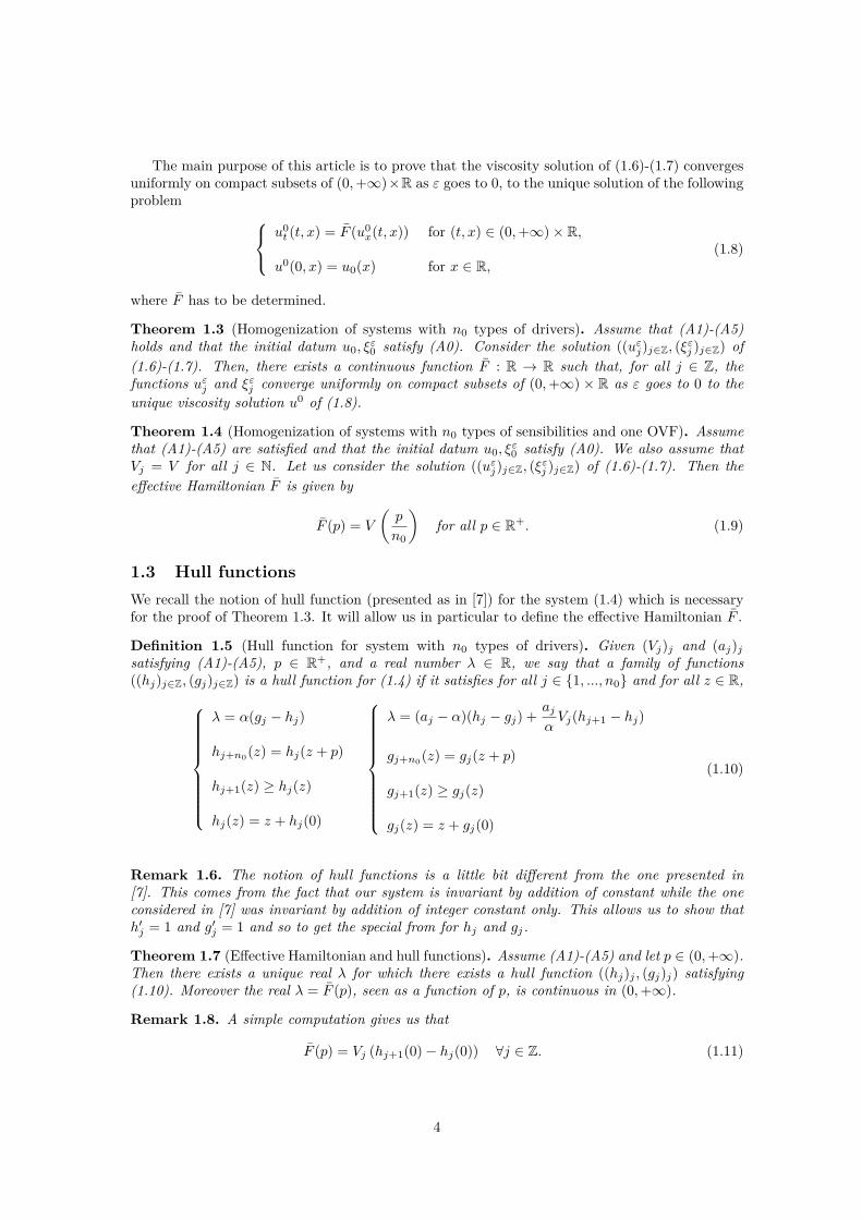
The main purpose of this article is to prove that the viscosity solution of (1.6)-(1.7) convergesuniformly on compact subsets of (0,+∞)×R as ε goes to 0, to the unique solution of the followingproblem u0

t (t, x) = F (u0x(t, x)) for (t, x) ∈ (0,+∞)× R,

u0(0, x) = u0(x) for x ∈ R,(1.8)

where F has to be determined.

Theorem 1.3 (Homogenization of systems with n0 types of drivers). Assume that (A1)-(A5)holds and that the initial datum u0, ξ

ε0 satisfy (A0). Consider the solution ((uεj)j∈Z, (ξεj )j∈Z) of

(1.6)-(1.7). Then, there exists a continuous function F : R → R such that, for all j ∈ Z, thefunctions uεj and ξεj converge uniformly on compact subsets of (0,+∞) × R as ε goes to 0 to theunique viscosity solution u0 of (1.8).

Theorem 1.4 (Homogenization of systems with n0 types of sensibilities and one OVF). Assumethat (A1)-(A5) are satisfied and that the initial datum u0, ξ

ε0 satisfy (A0). We also assume that

Vj = V for all j ∈ N. Let us consider the solution ((uεj)j∈Z, (ξεj )j∈Z) of (1.6)-(1.7). Then theeffective Hamiltonian F is given by

F (p) = V

(p

n0

)for all p ∈ R+. (1.9)

1.3 Hull functionsWe recall the notion of hull function (presented as in [7]) for the system (1.4) which is necessaryfor the proof of Theorem 1.3. It will allow us in particular to define the effective Hamiltonian F .

Definition 1.5 (Hull function for system with n0 types of drivers). Given (Vj)j and (aj)jsatisfying (A1)-(A5), p ∈ R+, and a real number λ ∈ R, we say that a family of functions((hj)j∈Z, (gj)j∈Z) is a hull function for (1.4) if it satisfies for all j ∈ 1, ..., n0 and for all z ∈ R,

λ = α(gj − hj)

hj+n0(z) = hj(z + p)

hj+1(z) ≥ hj(z)

hj(z) = z + hj(0)

λ = (aj − α)(hj − gj) + ajαVj(hj+1 − hj)

gj+n0(z) = gj(z + p)

gj+1(z) ≥ gj(z)

gj(z) = z + gj(0)

(1.10)

Remark 1.6. The notion of hull functions is a little bit different from the one presented in[7]. This comes from the fact that our system is invariant by addition of constant while the oneconsidered in [7] was invariant by addition of integer constant only. This allows us to show thath′j = 1 and g′j = 1 and so to get the special from for hj and gj.

Theorem 1.7 (Effective Hamiltonian and hull functions). Assume (A1)-(A5) and let p ∈ (0,+∞).Then there exists a unique real λ for which there exists a hull function ((hj)j , (gj)j) satisfying(1.10). Moreover the real λ = F (p), seen as a function of p, is continuous in (0,+∞).

Remark 1.8. A simple computation gives us that

F (p) = Vj (hj+1(0)− hj(0)) ∀j ∈ Z. (1.11)

4

1.4 Qualitative properties of the effective HamiltonianWe have the following results concerning F , and concerning the homogenized Hamilton-Jacobiequation (1.8).

Theorem 1.9 (Qualitative properties of F ). Assume (A1)-(A5). For any p ∈ (0,+∞), let F (p)denote the effective Hamiltonian given by Theorem 1.7. Then we have the following properties

(i) (Lower boundary) if p ≤ 2h0n0, we have

F (p) = 0.

(ii) (Upper boundary)

limp→+∞

F (p) = minj∈1,...,n0

(||Vj ||∞).

(iii) (Monotonicity) F is non-decreasing.

Remark 1.10. For example, an effective Hamiltonian can be of the form:

Figure 1: Schematic representation of the effective Hamiltonian.

Link with macroscopic models In the literature we can find different types of macroscopicmodels. But we will focus on the first order model LWR (Lighthill-Whitham-Richards) (for moreinformation on the LWR model see for instance [17]), which is defined by

∂tρ+ ∂y(ρv(ρ)) = 0, (1.12)

where ρ(t, y) is the density of vehicles at the point y ∈ R (physical point on the road) at timet ∈ (0,+∞), and v(ρ) is the average speed of vehicles. We call f(ρ) = ρv(ρ) the traffic flux. It canbe remarked that (1.12) uses Eulerian coordinates (y is physical point on the road). However, itwas proven by Wagner in [18] (for equations of gas dynamics) that the problem (1.12) is equivalentto

∂ts− ∂xv∗(s) = 0, (1.13)

where s(t, x) = 1/ρ is the spacing between the vehicles, x stands for the vehicle x (seen asa continuous variable) and v∗(s) = v(1/s). We can see that equation (1.13) uses Lagrangiancoordinates. Moreover, if we denote by u0(t, x) the position of the x vehicle, we have that (1.13)is equivalent (see [14]) to

∂tu0(t, x) = v∗

(∂xu

0) , (1.14)

5

with s(t, x) = ∂xu0(t, x). From this we can see that equation (1.8) is equivalent to a macroscopic

model of traffic flow of the LWR type, with

v(ρ) := F

(1ρ

).

Using Theorem 1.9, we can see that the flux of the macroscopic model, f(ρ) = ρv(ρ), satisfiessome of the properties presented in [17]:

1. f is a continuous function.

2. f(0) = f(ρmax) = 0, with ρmax = n0

h0.

1.5 Organisation of the articleIn Section 2 we give some results concerning viscosity solutions for systems. In Section 3, we proveTheorem 1.3 assuming Theorem 1.7. In Section 4 we give the results concerning the existence ofthe hull functions.

2 Viscosity SolutionsThis section is devoted to the definition and to useful results for viscosity solutions for systemslike (1.4). The reader is referred to the user’s guide of Crandall, Ishii, Lions [5] and the book ofBarles [2] for an introduction to viscosity solutions and to [11, 12, 15] and references therein forresults concerning viscosity solutions for weakly coupled systems.

2.1 DefinitionsWe consider for 0 < T ≤ +∞ the following Cauchy problem, for j ∈ Z , t > 0 and x ∈ R,

∂uj∂t

(t, x) = α(ξj(t, x)− uj(t, x))

∂ξj∂t

(t, x) = (aj − α)(uj(t, x)− ξj(t, x)) + ajαVj(uj+1(t, x)− uj(t, x))

uj+n0(t, x) = uj(t, x+ 1)

ξj+n0(t, x) = ξj(t, x+ 1),

(2.1)

with the initial condition

uj(0, x) = u0

(x+ j

n0

)and ξj(0, x) = ξ0

(x+ j

n0

). (2.2)

We recall the definition of the upper and lower semi-continuous envelopes, u∗ and u∗, of alocally bounded function u,

u∗(t, x) = lim sup(τ,y)→(t,x)

u(τ, y) and u∗(t, x) = lim inf(τ,y)→(t,x)

u(τ, y).

Definition 2.1 (Viscosity Solutions). Let T > 0, u0 : R → R and ξ0 : R → R satisfying (A0’).For all j, let uj : R+ × R→ R and ξj : R+ × R→ R be upper semi-continuous (resp. lower semi-continuous) locally bounded functions. We set Ω = (0, T ) × R. Let us consider that ((uj)j , (ξj)j)satisfies

∀j ∈ Z, ∀(t, x) ∈ Ω, uj+n0(t, x) = uj(t, x+ 1) and ξj+n0(t, x) = ξj(t, x+ 1).

6

-A function ((uj)j , (ξj)j) is a sub-solution (resp. a super-solution) of (2.1) on Ω if for all(t, x) ∈ Ω and for any test function ϕ ∈ C1(Ω) such that uj −ϕ attains a local maximum (resp. alocal minimum) at the point (t, x), we have

ϕt(t, x) ≤ α(ξj(t, x)− uj(t, x)) (resp. ≥), (2.3)

and for all (t, x) ∈ Ω, and any test function ϕ ∈ C1(Ω) such that ξj − ϕ attains a local maximum(resp. a local minimum) at the point (t, x), we have

ϕt(t, x) ≤ (aj − α)(uj(t, x)− ξj(t, x)) + aj

α Vj(uj+1(t, x)− uj(t, x)) (resp. ≥) (2.4)

-A function ((uj)j , (ξj)j) is a sub-solution (resp. a super-solution) of (2.1)-(2.2) if ((uj)j , (ξj)j)is a sub-solution (resp. a super solution) of (2.1) on Ω and if it satisfies moreover for all x ∈ R,j ∈ 1, ..., n0,

uj(0, x) ≤ u0

(x+ j

n0

)(resp. ≥) and ξj(0, x) ≤ ξ0

(x+ j

n0

)(resp. ≥).

-A function ((uj)j , (ξj)j) is a viscosity solution of (2.1) (resp. of (2.1)-(2.2)) if ((u∗j )j , (ξ∗j )j)is a sub-solution and (((uj)∗)j , ((ξj)∗)j) is a super solution of (2.1) (resp. of (2.1)-(2.2)).

2.2 Results for viscosity solutions of (2.1)Proposition 2.2 (Comparison Principle). Assume (A0) and (A1)-(A5). Let (uj , ξj) and (vj , ζj))be respectively a sub-solution and a super-solution of (2.1)-(2.2). We also assume that there is aconstant K > 0 such that for all j ∈ 1, ..., n0 and for all (t, x) ∈ [0;T ]× R, we have

uj(t, x) ≤ uj(0, x) +K(1 + t), ξj(t, x) ≤ ξj(0, x) +K(1 + t)

−vj(t, x) ≤ −vj(0, x) +K(1 + t), −ζj(t, x) ≤ −ξj(0, x) +K(1 + t).(2.5)

If

uj(0, x) ≤ vj(0, x) and ξj(0, x) ≤ ζj(0, x) for all x ∈ R, j ∈ Z,

then

uj(t, x) ≤ vj(t, x) and ξj(t, x) ≤ ζj(t, x) for all x ∈ R, j ∈ Z, t ∈ [0;T ].

Proof of Proposition 2.2.This proof is similar to the one of Proposition 2.2 in [7], because the system (2.1) is monotone

as the one studied in [7] thanks to assumption (A2), so we skip it.

We now give a comparison principle on bounded sets, to do this, we define, for a given point(t0, x0) ∈ (0, T )× R and for all r,R > 0, the set

Qr,R = (t0 − r, t0 + r)× (y0 −R, y0 +R).

Proposition 2.3 (Comparison principle on bounded sets). Assume (A1)-(A5). Let ((uj)j , (ξj)j)(resp. ((vj)j , (ζj)j)) be a sub-solution (resp. a super-solution) of (2.1) on the open set Qr,R ⊂(0, T )× R. Assume also that for all j ∈ 1, ..., n0,

uj ≤ vj and ξj ≤ ζj on Qr,R \ Qr,R,

then

uj ≤ vj and ξj ≤ ζj on Qr,R for j ∈ 1, ..., n0.

7

We now turn to the existence of a solution for equation (2.1). To do this we will use thefollowing lemma.

Lemma 2.4 (Existence of Barriers). Assume (A0) and (A1)-(A3). There exist a constant K1 > 0such that

((u+j (t, x))j , (ξ+

j (t, x))j) =((

u0

(x+ j

n0

)+K1t

)j

,

(ξ0

(x+ j

n0

)+K1t

)j

),

and

((u−j (t, x))j , (ξ−j (t, x))j) =((

u0

(x+ j

n0

)−K1t

)j

,

(ξ0

(x+ j

n0

)−K1t

)j

),

are respectively super and sub-solutions of (2.1)-(2.2) for all T > 0. Moreover, the constant K1can be chosen to be

K1 = maxj∈1,...,n0

(aj).Vmaxα

.

Proof. Let us prove that ((u+j (t, x))j , (ξ+

j (t, x)j)) is a super-solution of (2.1)-(2.2).First, using (A0) with ε = 1 we have for all j ∈ 1, ..., n0,

α(ξ+j (t, x)− u+

j (t, x)) = α

(ξ0

(x+ j

n0

)− u0

(x+ j

n0

))≤ Vmax ≤ K1,

and

(aj − α)(u+j (t, x)− ξ+

j (t, x)) + ajαVj(u+

j+1(t, x)− u+j (t, x)) ≤ max(aj)

αVmax ≤ K1, (2.6)

where we have used (A0) and the fact that for all j, ||Vj ||∞ ≤ Vmax.

By applying Perron’s method, joint to the comparison principle, we get the following result.

Theorem 2.5 (Existence and uniqueness of viscosity solutions for (2.1)). Assume (A0) and (A1)-(A5). Then there exists a unique solution ((uj)j , (ξj)j) of (2.1)-(2.2). Moreover, the functionsuj , ξj are continuous for all j ∈ Z.

We now prove that the cars remain in ordered during the evolution.

Theorem 2.6 (Ordering of the cars). Assume (A0) and (A1)-(A5). Let ((uj)j , (ξj)j) be a solutionof (2.1). Then uj and ξj are non-decresing with respect to j.

In order to do the proof of this theorem we need the following lemma.

Lemma 2.7 (Bound on time-derivative). Assume (A1)-(A5). Let ((uj)j , (ξj)j) be a solution of(1.4), with initial condition ((uj(0, x))j , (ξj(0, x))j) satisfying (A0). Then for all (t, x) ∈ [0, T ]×Rand for all j ∈ Z,

0 ≤ ξj(t, x)− uj(t, x) ≤ Vmaxα

.

Proof. Since ξj −uj is periodic in j it is sufficient to do this proof for j ∈ 1, ..., n0. We will onlydo the proof for the upper bound since the proof for the lower bound is similar.

8

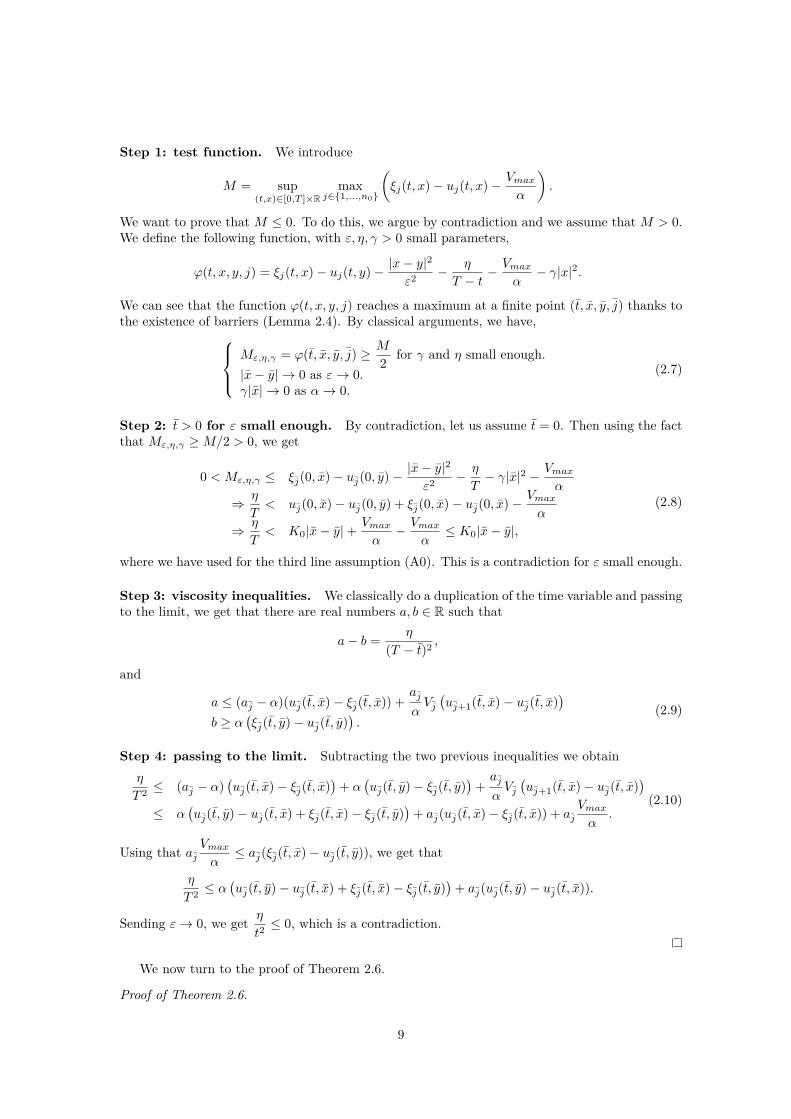
Step 1: test function. We introduce

M = sup(t,x)∈[0,T ]×R

maxj∈1,...,n0

(ξj(t, x)− uj(t, x)− Vmax

α

).

We want to prove that M ≤ 0. To do this, we argue by contradiction and we assume that M > 0.We define the following function, with ε, η, γ > 0 small parameters,

ϕ(t, x, y, j) = ξj(t, x)− uj(t, y)− |x− y|2

ε2 − η

T − t− Vmax

α− γ|x|2.

We can see that the function ϕ(t, x, y, j) reaches a maximum at a finite point (t, x, y, j) thanks tothe existence of barriers (Lemma 2.4). By classical arguments, we have,

Mε,η,γ = ϕ(t, x, y, j) ≥ M

2 for γ and η small enough.|x− y| → 0 as ε→ 0.γ|x| → 0 as α→ 0.

(2.7)

Step 2: t > 0 for ε small enough. By contradiction, let us assume t = 0. Then using the factthat Mε,η,γ ≥M/2 > 0, we get

0 < Mε,η,γ ≤ ξj(0, x)− uj(0, y)− |x− y|2

ε2 − η

T− γ|x|2 − Vmax

α

⇒ η

T< uj(0, x)− uj(0, y) + ξj(0, x)− uj(0, x)− Vmax

α

⇒ η

T< K0|x− y|+

Vmaxα− Vmax

α≤ K0|x− y|,

(2.8)

where we have used for the third line assumption (A0). This is a contradiction for ε small enough.

Step 3: viscosity inequalities. We classically do a duplication of the time variable and passingto the limit, we get that there are real numbers a, b ∈ R such that

a− b = η

(T − t)2 ,

and

a ≤ (aj − α)(uj(t, x)− ξj(t, x)) +ajαVj(uj+1(t, x)− uj(t, x)

)b ≥ α

(ξj(t, y)− uj(t, y)

).

(2.9)

Step 4: passing to the limit. Subtracting the two previous inequalities we obtainη

T 2 ≤ (aj − α)(uj(t, x)− ξj(t, x)

)+ α

(uj(t, y)− ξj(t, y)

)+ajαVj(uj+1(t, x)− uj(t, x)

)≤ α

(uj(t, y)− uj(t, x) + ξj(t, x)− ξj(t, y)

)+ aj(uj(t, x)− ξj(t, x)) + aj

Vmaxα

.(2.10)

Using that ajVmaxα≤ aj(ξj(t, x)− uj(t, y)), we get that

η

T 2 ≤ α(uj(t, y)− uj(t, x) + ξj(t, x)− ξj(t, y)

)+ aj(uj(t, y)− uj(t, x)).

Sending ε→ 0, we get η

t2≤ 0, which is a contradiction.

We now turn to the proof of Theorem 2.6.

Proof of Theorem 2.6.

9

Case 1: k0 ≥ 2h0n0. In this case we have for all j ∈ Z and y ∈ R,

2Vmaxα

= 2h0 ≤ u0

(y + j + 1

n0

)− u0

(y + j

n0

)Now, we would like to prove that uj(t, y) < uj+1(t, y) − h0. We argue by contradiction, let usassume that there exists a time

t∗ = inf t, s.t ∃i ∈ Z, y ∈ R s.t ui(t, y) = ui+1(t, y)− h0 .

Let us consider y ∈ R and i ∈ Z such that ui(t∗, y) = ui+1(t∗, y)− 2h0. By continuity, there existsa time t0 ∈ [0, t∗) such that

ui(t0, y) = ui+1(t0, y)− 2h0 and ui+1(t, y)− ui(t, y) ∈ [h0, 2h0] for all t ∈ [t0, t∗].

Let us now see the equation satisfied by (ui, ξi) for t ∈ [t0, t∗], using that Vi(ui+1(t, y)−ui(t, y)) = 0,

(ui)t(t, y) = α(ui(t, y)− ξi(t, y))

(ξi)t(t, y) = (ai − α)(ui(t, y)− ξi(t, y))

ui(t0, y) = ui+1(t0, y)− 2h0

ξi(t0, y) ≤ ui+1(t0, y)− 2h0 + Vmaxα

.

(2.11)

The last inequality is justified by Lemma 2.7. We now construct a super-solution for this systemby considering

ui(t, y) = Vmax

ai(1− e−ai(t−t0)) + ui+1(t0, y)− 2h0

ξi(t, y) = ui(t, y) + 1α (ui)t(t, y),

with the initial condition ui(t0, y) = ui+1(t0, y)− 2h0

ξi(t0, y) = ui+1(t0, y)− 2h0 + Vmax

α .

Since t0 < t∗, we have

ui(t∗, y) < Vmaxα− h0 + ui+1(t0, y)− h0

= ui+1(t0, y)− h0

≤ ui+1(t∗, y)− h0,

(2.12)

where we used for the first line the fact that 1 − eai(t∗−t0) < 1 and that α ≤ ai, for the secondline the fact that h0 = Vmax/α, and for the third line the fact that t∗ > t0 and Lemma 2.7 whichimplies that the uj are non-decreasing in t. Using the comparison principle for (2.11) yields

ui(t∗, y) ≤ ui(t∗, y) < ui+1(t∗, y)− h0. (2.13)

This is a contradiction with the definition of t∗. Therefore, we have for all j ∈ 1, ...., n0, for all(t, x) ∈ [0, T ]× R, that

uj(t, x) < uj+1(t, x)− h0.

10

Now from Lemma 2.7 we know that for all (t, x) ∈ (0,+∞)× R and for all j ∈ Z, Vmax ≥ α(ξj(t, x)− uj(t, x)) ≥ 0

Vmax ≥ α(ξj+1(t, x)− uj+1(t, x)) ≥ 0,

from which we can easily deduce that for all j ∈ Z, for all (t, x) ∈ [0, T ]× R, we have

ξj+1(t, x) ≥ ξj(t, x).

Case 2: 0 < k0 ≤ 2h0n0. We use the following lemma:

Lemma 2.8. Assume (A1)-(A5), let i ∈ Z, y ∈ R, and let 2h0 − k0/n0 ≥ δ > 0, also let usassume that

ui(0, y) = ui+1(0, y)− (2h0 − δ) and 0 ≤ ξi(0, y)− ui(0, y) ≤ 2h0 − δ2 , (2.14)

then we have

ui(t, y) ≤ ui+1(t, y) and ξi(t, y) ≤ ξi+1(t, y),

for all time t ∈ [0, T ] such that

ui+1(t, y)− ui(t, y) ≤ 2h0.

Proof. Let us denote by t, the time

t = inft s.t. ui+1(t, y)− ui(t, y) = 2h0,

then for all t ∈ [0, t], ui+1(t, y)−ui(t, y) ≤ 2h0, and (ui, ξi) is solution to the following system, fort ∈ [0, t]

(ui)t = α(ξi − ui)

(ξi)t = (ai − α)(ui − ξi)

ui(0, y) = ui+1(0, y)− (2h0 − δ)

ξi(0, y) ≤ ui+1(0, y)− 2h0 + δ + 2h0 − δ2 ,

We can construct a super-solution of this system by consideringui(t, y) = α

2h0 − δ2ai

(1− e−ait) + ui+1(0, y)− 2h0 + δ

ξi(t, y) = ui(t, y) + 1α

(ui)t(t, y).

(2.15)

Therefore, for all t ∈ [0, t], we have

ui+1(t, y)− ui(t, y) ≥ ui+1(0, y)− ui(t, y)≥ ui+1(0, y)− ui(t, y)

≥ 2h0 − δ − α2h0 − δ

2ai≥ 2h0 − δ −

2h0 − δ2

≥ 2h0 − δ2 ≥ 0,

(2.16)

11

where we have used for the first line the fact that ui+1 is non-decreasing in time (see Lemma 2.7),for the second line a comparison between ui and ui, for the third line the definition of ui(t, y) andthe fact that 1− e−ait ≤ 1, and for the fourth line the fact that α ≤ ai. Similarly, we have

ξi+1(t, y)− ξi(t, y) ≥ ui+1(t, y)− ξi(t, y)≥ ui+1(t, y)− ui(t, y)− 1

α(ui)t(t, y)

≥ 2h0 − δ2 − 2h0 − δ

2 ≥ 0,(2.17)

where we have used for the first line Lemma 2.7 and the fact that ξi ≥ ξi, for the second line thedefinition of ξ.

Using this lemma, we deduce that in the case where there exist i ∈ Z and y ∈ R such that

ui+1(0, y)− ui(0, y)2 ≤ Vmax

α= h0, (2.18)

we have

ui(t, y) ≤ ui+1(t, y) and ξi(t, y) ≤ ξi+1(t, y),

for all time t ∈ [0, t∗], where t∗ is defined by

t∗ = inft, ui+1(t, y)− ui(0, y) > 2h0.

We can then use the same proof as in Case 1 to deduce that

ui+1(t, y) ≥ ui(t, y) + h0 and ξi+1(t, y) ≥ ξi(t, y) for all t ≥ t∗.

3 ConvergenceThis section contains the proof of the main homogenization result (Theorem 1.3). This proof relieson the existence of hull functions and some properties of the effective Hamiltonian.

We recall two lemmas, necessary for the proof of Theorem 1.3. We begin by a first result whichis a direct consequence of Perron’s method and Lemma 2.4 (with a rescaling in ε).

Lemma 3.1 (Barriers uniform in ε). Assume (A1)-(A5) and (A0). Then there is a constantC > 0, such that for all ε > 0, the solution ((uεj)j , (ξεj )j) of (1.6)-(1.7) satisfies for all t > 0 andx ∈ R, ∣∣∣∣uεj(t, x)− u0

(x+ jε

n0

)∣∣∣∣ ≤ Ct and∣∣∣∣ξεj (t, x)− ξ0

(x+ jε

n0

)∣∣∣∣ ≤ Ct.Lemma 3.2 (ε-bounds on the gradient). Assume (A1)-(A5) and (A0). Then, the solution((uεj)j , (ξεj )j) of (1.6)-(1.7) satisfies for all t > 0 , x ∈ R ,z > 0 and j ∈ Z,

zk0 ≤ uεj(t, x+ z)− uεj(t, x) ≤ zK0, (3.1)

and

zk0 ≤ ξεj (t, x+ z)− ξεj (t, x) ≤ zK0. (3.2)

12

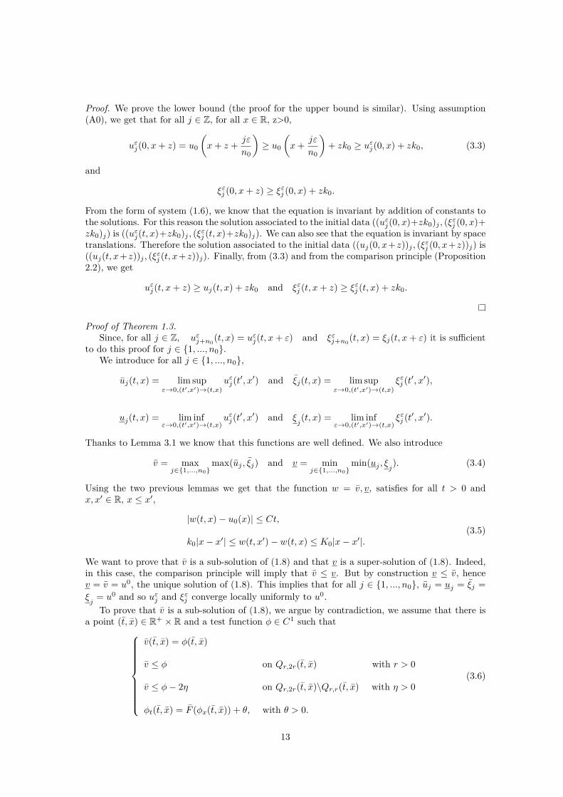
Proof. We prove the lower bound (the proof for the upper bound is similar). Using assumption(A0), we get that for all j ∈ Z, for all x ∈ R, z>0,

uεj(0, x+ z) = u0

(x+ z + jε

n0

)≥ u0

(x+ jε

n0

)+ zk0 ≥ uεj(0, x) + zk0, (3.3)

and

ξεj (0, x+ z) ≥ ξεj (0, x) + zk0.

From the form of system (1.6), we know that the equation is invariant by addition of constants tothe solutions. For this reason the solution associated to the initial data ((uεj(0, x)+zk0)j , (ξεj (0, x)+zk0)j) is ((uεj(t, x)+zk0)j , (ξεj (t, x)+zk0)j). We can also see that the equation is invariant by spacetranslations. Therefore the solution associated to the initial data ((uj(0, x+z))j , (ξεj (0, x+z))j) is((uj(t, x+z))j , (ξεj (t, x+z))j). Finally, from (3.3) and from the comparison principle (Proposition2.2), we get

uεj(t, x+ z) ≥ uj(t, x) + zk0 and ξεj (t, x+ z) ≥ ξεj (t, x) + zk0.

Proof of Theorem 1.3.Since, for all j ∈ Z, uεj+n0

(t, x) = uεj(t, x+ ε) and ξεj+n0(t, x) = ξj(t, x+ ε) it is sufficient

to do this proof for j ∈ 1, ..., n0.We introduce for all j ∈ 1, ..., n0,

uj(t, x) = lim supε→0,(t′,x′)→(t,x)

uεj(t′, x′) and ξj(t, x) = lim supε→0,(t′,x′)→(t,x)

ξεj (t′, x′),

uj(t, x) = lim infε→0,(t′,x′)→(t,x)

uεj(t′, x′) and ξj(t, x) = lim inf

ε→0,(t′,x′)→(t,x)ξεj (t′, x′).

Thanks to Lemma 3.1 we know that this functions are well defined. We also introduce

v = maxj∈1,...,n0

max(uj , ξj) and v = minj∈1,...,n0

min(uj , ξj). (3.4)

Using the two previous lemmas we get that the function w = v, v, satisfies for all t > 0 andx, x′ ∈ R, x ≤ x′,

|w(t, x)− u0(x)| ≤ Ct,

k0|x− x′| ≤ w(t, x′)− w(t, x) ≤ K0|x− x′|.(3.5)

We want to prove that v is a sub-solution of (1.8) and that v is a super-solution of (1.8). Indeed,in this case, the comparison principle will imply that v ≤ v. But by construction v ≤ v, hencev = v = u0, the unique solution of (1.8). This implies that for all j ∈ 1, ..., n0, uj = uj = ξj =ξj

= u0 and so uεj and ξεj converge locally uniformly to u0.To prove that v is a sub-solution of (1.8), we argue by contradiction, we assume that there is

a point (t, x) ∈ R+ × R and a test function φ ∈ C1 such that

v(t, x) = φ(t, x)

v ≤ φ on Qr,2r(t, x) with r > 0

v ≤ φ− 2η on Qr,2r(t, x)\Qr,r(t, x) with η > 0

φt(t, x) = F (φx(t, x)) + θ, with θ > 0.

(3.6)

13

We define p = φx(t, x) that according to (3.5) satisfies

0 < k0 ≤ p ≤ K0.

Using Theorem 1.7, we define the hull functions ((hj)j , (gj)j) associated to p such that

λ = F (p)

We now apply the perturbed test function method introduced by Evans [6] in terms here ofhull functions instead of correctors. Let us consider the following perturbed test functions forj ∈ 1, ..., n0,

φεj(t, x) = εhj

(φ(t, x)ε

)= φ(t, x) + εhj(0) and ψεj (t, x) = εgj

(φ(t, x)ε

)= φ(t, x) + εgj(0).

We define the family of test functions (φεj)j∈Z and (ψεj )j∈Z by using the relation

φεj+kn0(t, x) = φεj(t, x+ εk) and ψεj+kn0

(t, x) = ψεj (t, x+ εk).

We first want to prove that ((φεj)j , (ψεj )j) is a super-solution of (1.6) in a neighbourhood of(t, x).

To do this, we simply check the equations satisfied by the perturbed test functions, we denoteby z = φ(t,x)

ε to simply the notations. For j ∈ 1, ..., n0, we have

(φεj)t(t, x) = φt(t, x) + α(gj(z)− hj(z))− α(gj(z)− hj(z))

= α

ε(ψεj (t, x)− φεj(t, x)) + (φt(t, x)− λ)

= α

ε(ψεj (t, x)− φεj(t, x)) +

(φt(t, x)− φt(t, x) + θ

)≥ α

ε(ψεj (t, x)− φεj(t, x)),

where we have used the equations satisfied by the hull functions for the second line, the definitionof λ for the third line. For the fourth line we have used the fact that for r > 0 small enough, wehave

(φt(t, x)− φt(t, x) + θ

2)≥ 0, because θ > 0 and φ is C1. Similarly, we have

(ψεj )t(t, x) = φt(t, x)

= (aj − α)(hi(z)− gj(z)) + ajαVj(hj+1(z)− hj(z))− λ+ φt(t, x)

≥ (aj − α)ε

(φεj(t, x)− ψεj (t, x)) + ajαVj

(φεj+1(t, x)− φεj(t, x)

ε

)

+(φt(t, x)− φt(t, x) + θ

2

)

+θ

2 + ajα

[Vj(hj+1(z)− hj(z))− Vj

(φεj+1(t, x)− φεj(t, x)

ε

)].

It is then enough to prove that

θ

2 + ajα

[Vj(hj+1(z)− hj(z))− Vj

(φεj+1(t, x)− φεj(t, x)

ε

)]≥ 0.

14

If j + 1 ∈ 1, ..., n0, then,

hj(z) =φεj(t, x)

εand hj+1(z) =

φεj+1(t, x)ε

,

and the result is trivial.If j + 1 /∈ 1, ..., n0 then there is a k ∈ 1, ..., n0 such that k = k + lkn0,

hj+1(z) = h1+n0(z) = h1(z + p) = φ(t, x)ε

+ p+ h1(0),

φεj+1(t, x) = φεn0+1(t, x) = φε1(t, x+ ε) = φ(t, x+ ε) + εh1(0).= φ(t, x) + εp+ εh1(0) + +oε(ε).

This implies that

φεj+1(t, x)ε

= φ(t, x)ε

+ h1(0) + oε(1)= hj+1(z) + oε(1).

This allows us to see that for r > 0 small enough, we get

θ

2 + ajα

[Vj(hj+1(z)− hj(z))− Vj

(φεj+1(t, x)− φεj(t, x)

ε

)]≥ 0.

Getting a contradiction. By definition: φεj → φ and ψεj → φ as ε → 0. Moreover, uj ≤ v ≤φ− 2η on Qr,2r(t, x)\Qr,r(t, x) therefore, for ε small enough

uεj ≤ φεj − η ≤ φεj − η on Qr,2r(t, x)\Qr,r(t, x).

Similarly, we have

ξεj ≤ ψεj − η ≤ ψεj − η on Qr,2r(t, x)\Qr,r(t, x).

Using the comparison principle on bounded sets for (1.6), we get

uεj ≤ φεj − η and ξεj ≤ ψεj − η on Qr,r(t, x). (3.7)

Passing to the limit as ε → 0, we get v ≤ φ − η on Qr,r(t, x) and this contradicts the fact thatv(t, x) = φ(t, x).

Therefore v is a sub-solution of (1.8) on (0,+∞)×R. Similarly, v is a super-solution of the sameequation. Therefore, v = v = u0 and uj and ξj converge locally uniformly to u0 for j ∈ 1, ..., n0.

4 Ergodicity and construction of hull functionsIn this section, we construct the hull functions for (2.1). The construction follows the one of [7]but we use here the fact that the system is invariant by addition of constants. This allows us toget the particular form of the hull functions.

4.1 ErgodicityProposition 4.1 (Particular form of the solution of (2.1)). Assume (A1)-(A5) and let p > 0. Let((uj)j , (ξj)j) be the solution of (2.1) with u0(y) = ξ0(y) = py. Then ((uj)j , (ξj)j) satisfies

uj(t, y) = py + uj(t, 0) and ξj(t, y) = py + ξj(t, 0). (4.1)

15

Proof of Proposition 4.1. Using that equation (2.1) is invariant by space translations, invariantby addition of constants, and the fact that for all y, z ∈ R, j ∈ Z

u0

(y + z + j

n0

)− pz = u0

(y + j

n0

)and ξ0

(y + z + j

n0

)− pz = ξ0

(y + j

n0

),

we deduce, by the comparison principle, that

uj(t, y + z)− pz = uj(t, y) and ξj(t, y + z)− pz = ξj(t, y).

Taking y = 0, we deduce the result.

Proposition 4.2 (Ergodicity). Assume (A1)-(A5), let ((uj)j , (ξj)j) be a solution of (2.1) withinitial data u0(y) = ξ0(y) = py for some p > 0. Then there exists a constant λ ∈ R such that, forall (t, y) ∈ [0; +∞)× R, j ∈ 1, ..., n0,

|uj(t, 0)− λt| ≤ C1 and |ξj(t, 0)− λt| ≤ C1, (4.2)

and|λ| ≤ K1, (4.3)

with

C1 = 3p+ 4Vmaxα

, (4.4)

and K1 defined in Lemma 2.4.

The proof of Proposition 4.2 is done in different steps, it uses the following classical lemmafrom ergodic theory (see for instance [13]).

Lemma 4.3. Consider Λ : R+ → R a continuous function which is sub-additive, meaning that:for all t, s ≥ 0,

Λ(t+ s) ≤ Λ(t) + Λ(s).

Then Λ(t)t has a limit l as t→ +∞ and

l = inft>0

Λ(t)t. (4.5)

Proof of Proposition 4.2.The main idea of the proof is to control the time oscillations. To do this we will use the

following continuous functions for all T > 0,

λu+(T ) = supj∈1,...,n0

supt≥0

uj(t+ T, 0)− uj(t, 0)T

,

λu−(T ) = infj∈1,...,n0

inft≥0

uj(t+ T, 0)− uj(t, 0)T

,

and

λξ+(T ) = supj∈1,...,n0

supt≥0

ξj(t+ T, 0)− ξj(t, 0)T

,

16

λξ−(T ) = infj∈1,...,n0

inft≥0

ξj(t+ T, 0)− ξj(t, 0)T

.

We also introduce

λ+(T ) = sup(λu+(T ), λξ+(T )) and λ−(T ) = inf(λu−(T ), λξ−(T )).

To get the result, it suffices to prove that λ+(T ) and λ−(T ) have a common limit λ as T → +∞such that |λ±−λ| ≤

C1

T. To do this we would like to apply Lemma 4.3. Because of their definitions,

we know that T 7→ Tλu+(T ) and T 7→ Tλξ+(T ) are sub-additive, in the same way T 7→ −Tλu−(T )and T 7→ −Tλξ−(T ) are also sub-additive. Therefore if λu±(T ) and λξ±(T ) are finite, we will getthe convergence, and we will only have to prove that they have the same limit.

Step 1: λ+(T ) and λ−(T ) converge as T goes to +∞. We want to use Lemma 4.3. SinceT 7→ Tλu+, T 7→ Tλξ+, T 7→ −Tλu− and T 7→ −Tλξ− are sub-additive, we deduce that T 7→ Tλ+and T 7→ −Tλ− are sub-additive. It just remains to show that λ+ and λ− are bounded (to get afinite limit). Using Lemma 2.7, we get that for all j ∈ 1, ..., n0 and for all t, T > 0, we have

−K1 ≤ 0 ≤ uj(t+ T, 0)− uj(t, 0)T

≤ Vmax ≤ K1 (4.6)

and

−K1 ≤ −max(aj − α)Vmaxα≤ ξj(t+ T, 0)− ξj(t, 0)

T≤ Vmax

αmax

j∈1,...,n0(aj) ≤ K1, (4.7)

where we have used the equation satisfied by ξj and the facts that

−ajVmaxα≤ −(aj − α)Vmax

α≤ (aj − α)(uj(t, x)− ξj(t, x)) ≤ 0,

and

0 ≤ Vj(uj+1(t, x)− uj(t, x)) ≤ Vmax.

Step 2: Control on the time oscillations We now prove that λ+ and λ− have the samelimit. More precisely, we will prove that

|λ+(T )− λ−(T )| ≤ C1

T,

with C1 defined in Proposition 4.2.By definition of λ±(T ), for all ε > 0, there exists τ± and v± ∈ u1, ...., un, ξ1, ..., ξn such that∣∣∣∣λ±(T )− v±(τ± + T, 0)− v±(τ±, 0)

T

∣∣∣∣ ≤ εLet us set for all j ∈ 1, ..., n0,

∆uj = uj(τ+, 0)− uj(τ−, 0), ∆ξ

j = ξj(τ+, 0)− ξj(τ−, 0)

and

∆ = supj∈1,...,n0

sup(∆uj ,∆

ξj).

Using Proposition 4.1, we have

uj(τ+, y) = uj(τ−, y) + uj(τ+, 0)− uj(τ−, 0) ≤ uj(τ−, y) + ∆

17

and

ξj(τ+, y) = ξj(τ−, y) + ξj(τ+, 0)− ξj(τ−, 0) ≤ ξj(τ−, y) + ∆.

Using the comparison principle we get

uj(τ+ + T, y) ≤ uj(τ− + T, y) + ∆ (4.8)

and

ξj(τ+ + T, y) ≤ ξj(τ− + T, y) + ∆. (4.9)

Now we would like to estimate ∆, Let us assume that the maximum in ∆ is reached for the indexj. We then have for all j ∈ 1, ..., n0,

∆ ≤ uj(τ+, 0)− uj(τ−, 0) + 2Vmaxα

≤ uj+n0(τ+, 0)− uj−n0(τ−, 0) + 2Vmaxα

≤ uj(τ+, 1)− uj(τ−,−1) + 2Vmaxα

≤ uj(τ+, 0)− uj(τ−, 0) + 2Vmaxα

+ 2p,

(4.10)

where we have used for the first line Lemma 2.7 (to compare uj and ξj), for the second line, thefact that (uj)j is non-decreasing in j, for the third line the periodicity of the function uj , and forthe last line we have used Proposition 4.1. Similarly we have

∆ ≤ ξj(τ+, 0)− ξj(τ−, 0) + 2Vmaxα

+ 2p.

We now inject this results in (4.8) and (4.9), with y = 0, to obtain

uj(τ+ + T, 0)− uj(τ+, 0) ≤ uj(τ− + T, 0)− uj(τ−, 0) + 2Vmaxα

+ 2p,

and

ξj(τ+ + T, 0)− ξj(τ+, 0) ≤ ξj(τ− + T, 0)− ξj(τ−, 0) + 2Vmaxα

+ 2p.

Using this two results we get that

v+(τ+ + T, 0)− v+(τ+, 0) ≤ v−(τ− + T, 0)− v−(τ−, 0) + 4Vmaxα

+ 3p,

where the possible comparison between ξj and uj adds an additional 2Vmax/α, and the possiblecomparison between uj and uk adds an additional p. This implies that

Tλ+(T ) ≤ Tλ−(T ) + 2εT + C1.

Since this is true for all ε > 0, we get

|λ+(T )− λ−(T )| ≤ C1

T. (4.11)

18

Step 3: Conclusion. From the previous step we know that λ± have the same limit. Let usdenote it by λ, and by Lemma 4.3 we have, for all T > 0,

λ−(T ) ≤ λ ≤ λ+(T ).

Using (4.11), we deduce that

|λ± − λ| ≤C1

T. (4.12)

4.2 Construction of hull functionsWe now would like to prove the existence of time-space global solutions of (2.1).

Proposition 4.4. Let p > 0 and assume (A1)-(A5). Then, there exist some constants((u∞j (0, 0))j , (ξ∞j (0, 0))j) and a real number λ ∈ R such that for all (τ, y) ∈ R2,((

u∞j (τ, y))j,(ξ∞j (τ, y)

)j

)=((py + λτ + u∞j (0, 0)

)j,(py + λτ + ξ∞j (0, 0)

)j

),

is a solution of (2.1). These constants satisfy, for all j ∈ Z,

u∞j+1(0, 0) ≥ u∞j (0, 0) and ξ∞j+1(0, 0) ≥ ξ∞j (0, 0). (4.13)

The interest of this result is that if we consider for all z ∈ R,hj(z) = z + u∞j (0, 0) if j ∈ 1, ..., n0

hj+n0(z) = hj(z + p),

gj(z) = z + ξ∞j (0, 0) if j ∈ 1, ..., n0

gj+n0(z) = gj(z + p),(4.14)

then we have directly the following result.

Corollary 4.5. (Existence of hull functions). Assume (A1)-(A5), then there exists λ ∈ R suchthat there exist a hull function ((hj)j , (gj)j) defined as in Definition 1.5.

Proof of Proposition 4.4.

Step 1: construction of a solution. In this step, we use the functions ((uj)j , (ξj)j) solutionof (2.1) with u0(y) = ξ0(y) = py. For m ∈ R, we consider

umj (t, 0) = uj(t+m, 0)− λm and ξmj (t, 0) = ξj(t+m, 0)− λm.

Since the equation is invariant by addition of constants and by time-translations, we deduce that((umj (t, y) = py + umj (t, 0)

)j,(ξmj (t, y) = py + umj (t, 0)

)j

), (4.15)

is a solution of (2.1). Moreover, umj is Lipschitz continuous in time thanks to Lemma 2.7 andas a consequence ξmj is also Lipschitz continuous in time. Therefore we can use Ascoli Theoremto deduce that there is a sub-sequence ((umj )j , (ξmj )j) converging uniformly on compact sets to aLipschitz continuous function ((u∞j )j , (ξ∞j )j) which satisfies, for all k ∈ R,

u∞j (t+ k, 0) = u∞j (t, 0) + λk

u∞j (t, y) = py + u∞j (t, 0)

u∞j+1 ≥ u∞j

ξ∞j (t+ k, 0) = ξ∞j (t, 0) + λk

ξ∞j (t, y) = py + ξ∞j (t, 0)

ξ∞j+1 ≥ ξ∞j .

(4.16)

19

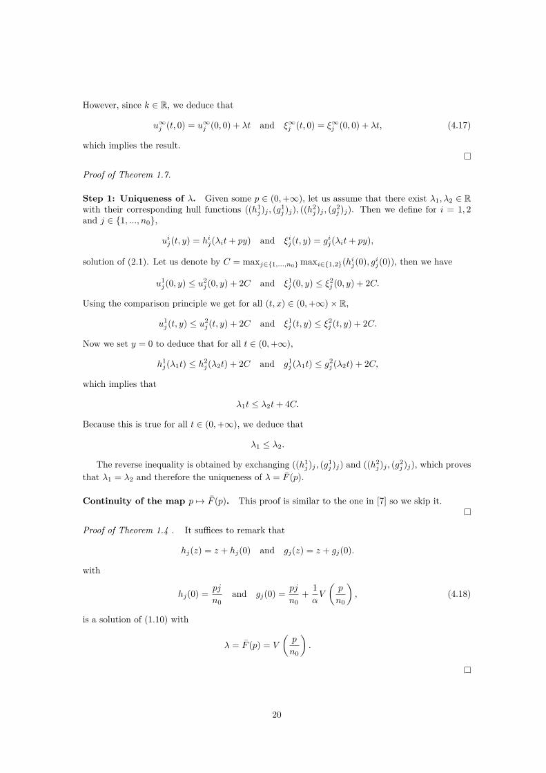
However, since k ∈ R, we deduce that

u∞j (t, 0) = u∞j (0, 0) + λt and ξ∞j (t, 0) = ξ∞j (0, 0) + λt, (4.17)

which implies the result.

Proof of Theorem 1.7.

Step 1: Uniqueness of λ. Given some p ∈ (0,+∞), let us assume that there exist λ1, λ2 ∈ Rwith their corresponding hull functions ((h1

j )j , (g1j )j), ((h2

j )j , (g2j )j). Then we define for i = 1, 2

and j ∈ 1, ..., n0,

uij(t, y) = hij(λit+ py) and ξij(t, y) = gij(λit+ py),

solution of (2.1). Let us denote by C = maxj∈1,...,n0maxi∈1,2(hij(0), gij(0)), then we have

u1j (0, y) ≤ u2

j (0, y) + 2C and ξ1j (0, y) ≤ ξ2

j (0, y) + 2C.

Using the comparison principle we get for all (t, x) ∈ (0,+∞)× R,

u1j (t, y) ≤ u2

j (t, y) + 2C and ξ1j (t, y) ≤ ξ2

j (t, y) + 2C.

Now we set y = 0 to deduce that for all t ∈ (0,+∞),

h1j (λ1t) ≤ h2

j (λ2t) + 2C and g1j (λ1t) ≤ g2

j (λ2t) + 2C,

which implies that

λ1t ≤ λ2t+ 4C.

Because this is true for all t ∈ (0,+∞), we deduce that

λ1 ≤ λ2.

The reverse inequality is obtained by exchanging ((h1j )j , (g1

j )j) and ((h2j )j , (g2

j )j), which provesthat λ1 = λ2 and therefore the uniqueness of λ = F (p).

Continuity of the map p 7→ F (p). This proof is similar to the one in [7] so we skip it.

Proof of Theorem 1.4 . It suffices to remark that

hj(z) = z + hj(0) and gj(z) = z + gj(0).

with

hj(0) = pj

n0and gj(0) = pj

n0+ 1αV

(p

n0

), (4.18)

is a solution of (1.10) with

λ = F (p) = V

(p

n0

).

20

5 Qualitative properties of the effective HamiltonianProof of Theorem 1.9.

Step 1: proof of the lower bound . If we have p ≤ 2h0n0, then we can see that((hj(z))j , (gj(z))j

)=((

z + pj

n0

)j

,

(z + pj

n0

)j

),

is a hull function for λ = 0. In fact we have

λ = α(gj(z)− hj(z)) = 0,

and

λ = (aj − α)(hj(z)− gj(z)) + ajαVj

(p

n0

)= 0,

where we have used assumption (A4). Now by uniqueness of the effective Hamiltonian we havethat F (p) = 0.

Step 2: proof of the upper bound. A simple computation gives

F (p) = Vj(hj+1(0)− hj(0)), for all j ∈ Z

However, we also know that hj+1(0) ≥ hj(0) and that hj+n0(0) = hj(0) + p this means that thereexists a i ∈ j, ..., j + n0 such that hi+1(0) − hi(0) ≥ p/n0. Therefore, using the fact that Vi isnon-decreasing, we have

Vi

(p

n0

)≤ F (p) ≤ min

j∈1,...,n0(||Vj ||∞). (5.1)

Passing to the limit as p goes to +∞, we get the desired result.

Step 3: proof of the monotonicity. Let p1, p2 ∈ (0,+∞), and let λ1 = F (p1), λ2 = F (p2)be their respective effective Hamiltonians, each associated to the hull functions ((h1

j )j , (g1j )j) and

((h2j )j , (g2

j )j). We assume that p2 > p1. Therefore, we have

h1n0

(0)− h10(0) = p1 < p2 = h2

n0(0)− h2

0(0).

From this, we can deduce that there exists an integer k ∈ 0, ..., n0 − 1 such that

h1k+1(0)− h1

k(0) < h2k+1(0)− h2

k(0).

Now, using the monotonicity of Vk, we get,

Vk(h1k+1(0)− h1

k(0))≤ Vk

(h2k+1(0)− h2

k(0)),

which implies that λ1 ≤ λ2. Therefore the function F is non decreasing.

ACKNOWLEDGMENTSThis work was partially supported by ANR IDEE (ANR-2010-0112-01) and ANR HJNet (ANR-

12-BS01-0008-01).

21

References[1] M. Bando, K. Hasabe, A. Nakayama, A. Shibata, Y. Sugiyama, Dynamical model of traffic

congestion and numerical simulation, The American Physical Society, vol. 51 num. 2, February1995, pp. 1035–1042.

[2] G. Barles, Solutions de viscosité des équations de Hamilton-Jacobi, vol; 17 of Mathématiques& Applications (Berlin) [Mathematics & Applications], Springer-Verlag, Paris, 1994.

[3] M. Batista, E. Twrdy, Optimal velocity functions for car-following models, J. Zheijang Univ-Sci A (Appl. Phys. & Eng.), 2010, pp. 520-529.

[4] F. Camilli, O. Ley, and P. Loreti, Homogenization of monotone systems of Hamilton-Jacobiequations, ESAIM Control Optim. Calc. Var., 16 (2010), pp. 58–76.

[5] M. G. Crandall, H. Ishii, and P.-L. Lions, User’s guide to viscosity solutions of second orderpartial differential equations, Bull. Amer. Math. Soc. (N.S.), 27 (1992), pp. 1-67.

[6] L. C. Evans, The perturbed test function method for viscosity solutions of nonlinear PDE,Proc. Roy. Soc. Edinburgh Sect. A, 111 (1989), pp. 1057-1097.

[7] N. Forcadel, C. Imbert et R. Monneau , Homogenization of accelerated Frenkel-KontorovaModels with n types of particles, Transactions of the American Mathematical Society, pp.6187–6227, 2012.

[8] N. Forcadel, C. Imbert et R. Monneau , Homogenization of some particle systems with two-body interactions and of the discolation dynamics,Discrete Contin. Dyn. Syst., 23 (2009), pp.785-826.

[9] N. Forcadel, C. Imbert et R. Monneau , Homogenization of fully overdamped Frenkel-Kontorova models, J. Differential Equations, 246 (2009), pp. 1057–1097.

[10] C. Imbert, R. Monneau, and E. Rouy, Homogenization of first order equations with (u/ε)-periodic Hamiltonians. II. Application to dislocations dynamics, Comm. Partial DifferentialEquations, 33 (2008), pp. 479-516.

[11] H. Ishii , Perron’s method for monotone systems of second-order elliptic partial differentialequations, Differential Integral Equations, 5 (1992), pp. 1-24.

[12] H. Ishii and S. Koike, Viscosity solutions for monotone systems of second-order elliptic PDEs,Comm. Partial Differential Equations, 16 (1991), pp. 1095-1128.

[13] T. Kato, Perturbation theory for linear operators, Classics in Mathematics, Springer-Verlag,Berlin, 1995. Reprint of the 1980 edition.

[14] L. Leclercq, J. Laval and E. Chevallier The Lagrangian coordinates and what it means forfirst order traffic flow models, Transportation and Traffic Theory 2007, pp 735-753.

[15] S. M. Lenhart, Viscosity solutions for weakly coupled systems of first-order partial differentialequations, J. Math. Anal. Appl., 131 (1988), pp. 180-193.

[16] P.-L. Lions, G.C. Papanicolaou, S.R.S. Varadhan, Homogenisation of Hamilton-Jacobi equa-tions, unpublished preprint, (1986).

[17] B. Piccoli and M. Garavello Traffic Flow on Networks, vol. 1 of AIMS on Applied Math.Chapter 3 pp 47-70.

[18] D. Wagner, Equivalence of the Euler and Lagrangian equations of gas dynamics for weaksolutions, J. Differential Equations, 68, 118-136.

22