Homogenization of a viscoelastic model for plant cell wall ... · equations, compered to classical...

ESAIM: COCV 23 (2017) 1447–1471 ESAIM: Control, Optimisation and Calculus of VariationsDOI: 10.1051/cocv/2016060 www.esaim-cocv.org

HOMOGENIZATION OF A VISCOELASTIC MODEL FOR PLANT CELL WALLBIOMECHANICS ∗

Mariya Ptashnyk1

and Brian Seguin2

Abstract. The microscopic structure of a plant cell wall is given by cellulose microfibrils embedded ina cell wall matrix. In this paper we consider a microscopic model for interactions between viscoelasticdeformations of a plant cell wall and chemical processes in the cell wall matrix. We consider elasticdeformations of the cell wall microfibrils and viscoelastic Kelvin–Voigt type deformations of the cellwall matrix. Using homogenization techniques (two-scale convergence and periodic unfolding methods)we derive macroscopic equations from the microscopic model for cell wall biomechanics consisting ofstrongly coupled equations of linear viscoelasticity and a system of reaction-diffusion and ordinarydifferential equations. As is typical for microscopic viscoelastic problems, the macroscopic equationsgoverning the viscoelastic deformations of plant cell walls contain memory terms. The derivation ofthe macroscopic problem for the degenerate viscoelastic equations is conducted using a perturbationargument.

Mathematics Subject Classification. 35B27, 35Q92, 35Kxx, 74Qxx, 74A40, 74D05.

Received November 10, 2015. Accepted August 31st, 2016.

1. Introduction

To obtain a better understanding of the mechanical properties and development of plant tissues it is importantto model and analyse the interactions between the chemical processes and mechanical deformations of plantcells. The main feature of plant cells are their walls, which must be strong to resist high internal hydrostaticpressure (turgor pressure) and flexible to permit growth. The biomechanics of plant cell walls is determinedby the cell wall microstructure, given by microfibrils, and the physical properties of the cell wall matrix. Theorientation of microfibrils, their length, high tensile strength, and interactions with wall matrix macromoleculesstrongly influence the wall’s stiffness. It is also supposed that calcium-pectin cross-linking chemistry is one ofthe main regulators of cell wall elasticity and extension [30]. Pectin can be modified by the enzyme pectinmethylesterase (PME), which removes methyl groups by breaking ester bonds. The de-esterified pectin is ableto form calcium-pectin cross-links, and so stiffen the cell wall and reduce its expansion, see e.g. [29]. It hasbeen shown that the modification of pectin by PME and the control of the amount of calcium-pectin cross-links

Keywords and phrases. Homogenization, two-scale convergence, periodic unfolding method, viscoelasticity, plant modelling.

∗ M. Ptashnyk and B. Seguin gratefully acknowledge the support of the EPSRC First Grant EP/K036521/1 “Multiscale mod-elling and analysis of mechanical properties of plant cells and tissues”.1 Department of Mathematics, University of Dundee. Dundee, DD1 4HN, UK. [email protected] Department of Mathematics and Statistics, Loyola University Chicago, 60660 Chicago, USA. [email protected]

c© M. Ptashnyk and B. Seguin. Published by EDP Sciences, SMAI 2017

This is an Open Access article distributed under the terms of the Creative Commons Attribution License (http://creativecommons.org/licenses/by/4.0),which permits unrestricted use, distribution, and reproduction in any medium, provided the original work is properly cited.

https://doi.org/10.1051/cocv/2016060

http://www.esaim-cocv.org

http://creativecommons.org/licenses/by/4.0/

http://creativecommons.org/licenses/by/4.0

1448 M. PTASHNYK AND B. SEGUIN

greatly influence the mechanical deformations of plant cell walls [23,24], and the interference with PME activitycauses dramatic changes in growth behavior of plant cells and tissues [31].

To address the interactions between microstructure, chemistry and mechanics, in the microscopic model forplant cell wall biomechanics we consider the influence of the microscopic structure, associated with the cellulosemicrofibrils, and the calcium-pectin cross-links on the mechanical properties of plant cell walls. We model thecell wall as a three-dimensional continuum consisting of a polysaccharide matrix and cellulose microfibrils. It wasobserved experimentally that plant cell wall microfibrils are anisotropic, see e.g. [10], and the cell wall matrix, inaddition to elastic deformations, exhibits viscous behaviour, see e.g. [14]. Hence we model the cell wall matrixas a linearly viscoelastic Kelvin–Voigt material, whereas microfibrils are modelled as an anisotropic linearlyelastic material. Within the matrix, we consider the dynamics of the enzyme PME, methylesterfied pectin,demethylesterfied pectin, calcium ions, and calcium-pectin cross-links. A model for plant cell wall biomechanicsin which the cell wall matrix was assumed to be linearly elastic was derived and analysed in [26]. The interplaybetween the mechanics and the cross-link dynamics comes in by assuming that the elastic and viscous propertiesof the cell wall matrix depend on the density of the cross-links and that stress within the cell wall can breakcalcium-pectin cross-links. The stress-dependent opening of calcium channels in the cell plasma membraneis addressed in the flux boundary conditions for calcium ions. The resulting microscopic model is a system ofstrongly coupled four diffusion-reaction equations, one ordinary differential equation, and the equations of linearviscoelasticity. Since only the cell wall matrix is viscoelastic we obtain degenerate elastic-viscoelastic equations.In our model we focus on the interactions between the chemical reactions within the cell wall and its deformationand, hence, do not consider the growth of the cell wall.

To analyse the macroscopic mechanical properties of the plant cell wall we rigorously derive macroscopic equa-tions from the microscopic description of plant cell wall biomechanics. The two-scale convergence, e.g. [4, 21],and the periodic unfolding method, e.g. [7,8], are applied to obtain the macroscopic equations. For the viscoelas-tic equations the macroscopic momentum balance equation contains a term that depends on the history of thestrain represented by an integral term (fading memory effect). Due to the coupling between the viscoelasticproperties and the biochemistry of a plant cell wall, the elastic and viscous tensors depend on space and timevariables. This fact introduces additional complexity in the derivation and in the structure of the macroscopicequations, compered to classical viscoelastic equations.

The main novelty of this paper is the multiscale analysis and derivation of the macroscopic problem from amicroscopic description of the mechanical and chemical processes. This approach allows us to take into accountthe complex microscopic structure of a plant cell wall and to analyse the impact of the heterogeneous distributionof cell wall structural elements on the mechanical properties of plants. The main mathematical difficulty arisesfrom the strong coupling between the equations of linear viscoelasticity for cell wall mechanics and the systemof reaction-diffusion and ordinary differential equations for the chemical processes in the wall matrix. Alsothe degeneracy of the viscoelastic equations, due to the fact that only the cell wall matrix is assumed to beviscoelastic and microfibrils are assumed to be elastic, induces additional technical difficulties in the multiscaleanalysis of the microscopic model. To derive the macroscopic equations for the viscoelastic model for cell wallbiomechanics we consider perturbed equations by introducing an inertial term. Once the macroscopic problemof the perturbed equations is derived, the perturbation parameter is sent to zero. By showing that the limitproblem (as the perturbation parameter tends to zero) of the two-scale macroscopic problem for the perturbedmicroscopic equations is the same as the two-scale macroscopic problem for the original microscopic equations, weobtain the effective homogenized equations for the original viscoelastic problem coupled with reaction-diffusionand ordinary differential equations. A perturbation approach, by considering a viscosity term multiplied by asmall perturbation parameter in the elastic inclusions, was also used in [11] to derive a macroscopic model foran elastic-viscoelastic problem.

A multiscale analysis of the viscoelastic equations with time-independent coefficients was considered previ-ously in [12,13,18,27]. Macroscopic equations for scalar elastic-viscoelastic equations with time-independent coef-ficients were derived in [11] by applying the H-convergence method [19]. A microscopic viscoelastic Kelvin–Voigt

HOMOGENIZATION OF A VISCOELASTIC MODEL FOR PLANT CELL WALL BIOMECHANICS 1449

model with time-dependent coefficients in the context of thermo-viscoelasticity was analysed in [1] and macro-scopic equations were derived by applying the method of asymptotic expansion.

The paper is organised as follows. In Section 2 we formulate a mathematical model for plant cell wallbiomechanics in which the cell wall matrix is assumed to be viscoelastic. In Section 3 we summarise the mainresults of the paper. The well-possedness of the microscopic model is shown in Section 4. The multiscale analysisof the microscopic model is conducted in Section 5.

2. Microscopic model for viscoelastic deformations of plant cell walls

The main feature of plant cells are their walls, which must be strong to resist high internal hydrostaticpressure and flexible to permit the growth. To better understand the interplay between these in some senseconflicting functions, we consider a mathematical model describing the interactions between the mechanicalproperties and the chemical processes in cell walls, surrounding plant cells. Plant cell walls are separated fromthe inside of the cell by the plasma membrane, modelled as an internal boundary of the cell wall (see Fig. 1a).Individual cells in plant tissues are joined together by a pectin network of middle lamella. The primary wall of aplant cell consists mainly of oriented cellulose microfibrils imbedded in the cell wall matrix, which is composed ofpectin, hemicellulose, structural proteins, and water. It was observed experimentally that in addition to elasticdeformations the plant cell wall matrix exhibits viscoelastic behaviour [14]. Hence, in contrast to the modelconsidered in [26], here we assume that the deformations of the plant cell wall matrix are determined by theequations of linear viscoelasticity.

To model mechanical deformations of plant cell walls, we consider a domain Ω = (0, a1) × (0, a2) × (0, a3)representing a flat section of a cell wall, where ai, with i = 1, 2, 3, are positive numbers. We assume that themicrofibrils are oriented in the x3-direction (see Fig. 1b). We shall distinguish between six disjoint parts of theboundary ∂Ω of the domain Ω. The interior boundary ΓI = {0} × (0, a2) × (0, a3) represents the cell plasmamembrane, the exterior boundary ΓE = {a1} × (0, a2) × (0, a3) denotes the side of the cell wall which is incontact with the middle lamella, on the top and bottom boundaries ΓU = (0, a1) × {0} × (0, a3) ∪ (0, a1) ×{a2}× (0, a3) we will prescribe traction boundary conditions, reflecting the turgor pressure. On the boundariesΓP = (0, a1) × (0, a2) × {0} ∪ (0, a1) × (0, a2) × {a3} we consider periodic boundary conditions.

To determine the microscopic structure of the cell wall given by cell wall microfibrils, we consider Y =(0, 1)2 × (0, a3) and define Y = (0, 1)2, together with the subdomain YF , with YF ⊂ Y , and YM = Y \ YF . ThenYF = YF × (0, a3) and YM = YM × (0, a3) represent the cell wall microfibrils and cell wall matrix, rescaled tothe ‘unit cell’ Y (see Fig. 1c). We also define Γ = ∂YF ∩ ∂YM and Γ = ∂YF ∩ ∂YM .

We assume that the microfibrils in the cell wall are distributed periodically and have a diameter on the orderof ε, where the small parameter ε characterise the size of the microstructure, i.e. the ratio between the diameterof the microfibrils and the thickness of the cell wall. The domains

ΩεF =

⋃ξ∈Z2

{ε(YF + ξ) × (0, a3) | ε(Y + ξ) ⊂ (0, a1) × (0, a2)

}and Ωε

M = Ω \ΩεF

denote the parts of Ω occupied by the microfibrils and by the cell wall matrix, respectively. The boundarybetween the cell wall matrix and the microfibrils is denoted by

Γ ε = ∂ΩεM ∩ ∂Ωε

F .

We adopt the following notation: ΩT = (0, T )×Ω, ΩεM,T = (0, T )×Ωε

M , ΓI,T = (0, T )×ΓI, Γ εT = (0, T )×Γ ε,

ΓU ,T = (0, T )× ΓU , ΓE,T = (0, T ) × ΓE , and ΓEU ,T = (0, T ) × (ΓE ∪ ΓU ), and define

W(Ω) = {u ∈ H1(Ω; R3)∣∣ ∫

Ω

u dx = 0,∫

Ω

[(∇u)12 − (∇u)21] dx = 0 and u is a3-periodic in x3},

V(ΩεM ) = {n ∈ H1(Ωε

M )∣∣ n is a3-periodic in x3}.


)c()b()a(

cell nucleus

�

mitochandrion

�

vacule

�

cell wall

�

middle lamella

�

plasma membrane

�

ΓI

�

ΓE

ΩεF

�

ΩεM

�

� �a1

�

�

a2

�

�

a3��

1

�YM

�YF �

�

a3

�

�

1

ΓU

ΓU�

Figure 1. (a) A schematic of a plant cell with an indication of the domain Ω as a part of thecell wall. (b) A depiction of the domain Ω with the subsets representing the cell wall matrixΩε

M and the microfibrils ΩεF . The (hidden) surface ΓI corresponds to the plasma membrane

and is in contact with the interior of the cell, the surface ΓE is facing the outside of the celland is in contact with the middle lamella, and ΓU is the union of the surfaces on the top andbottom of Ω. (c) A depiction of the ‘unit cell’ Y .

By Korn’s second inequality, the L2-norm of the strain defines a norm on W(Ω)

‖u‖W(Ω) = ‖e(u)‖L2(Ω) for all u ∈ W(Ω),

see e.g. [6, 17, 22]. For more details see also [26].

The microscopic model for elastic-viscoelastic deformations uε of plant cell walls and for the densities ofesterified pectin pε

1, PME enzyme pε2, de-esterified pectin nε

1, calcium ions nε2, and calcium-pectin cross-links bε

reads

⎧⎪⎪⎪⎪⎪⎪⎨⎪⎪⎪⎪⎪⎪⎩

div (Eε(bε, x)e(uε) + Vε(bε, x)∂te(uε)) = 0 in ΩT ,

(Eε(bε, x)e(uε) + Vε(bε, x)∂te(uε))ν = −pIν on ΓI,T ,

(Eε(bε, x)e(uε) + Vε(bε, x)∂te(uε))ν = f on ΓEU ,T ,

uε a3-periodic in x3,

uε(0, x) = u0(x) in Ω,

(2.1)

and

∂tpε = div(Dp∇pε) − Fp(pε) in ΩεM,T ,

∂tnε = div(Dn∇nε) + Fn(pε,nε) + Rn(nε, bε,Nδ(e(uε))) in ΩεM,T ,

∂tbε = Rb(nε, bε,Nδ(e(uε))) in Ωε

M,T ,

(2.2)


where pε = (pε1, p

ε2)T , nε = (nε

1, nε2)T , and div(Dp∇pε) = (div(D1

p∇pε1), div(D2

p∇pε2))T , and div(Dn∇nε) =

(div(D1n∇nε

1), div(D2n∇nε

2))T , together with the initial and boundary conditions

Dp∇pε ν = Jp(pε) on ΓI,T ,

Dp∇pε ν = −γppε on ΓE,T ,

Dn∇nε ν = Nδ(e(uε))G(nε) on ΓI,T ,

Dn∇nε ν = Jn(nε) on ΓE,T ,

Dp∇pε ν = 0, Dn∇nε ν = 0 on Γ εT and ΓU ,T ,

pε, nε a3-periodic in x3,

pε(0, x) = p0(x), nε(0, x) = n0(x), bε(0, x) = b0(x) in ΩεM .

(2.3)

Here Nδ(e(uε)), defined as

Nδ(e(uε)) =

(−∫

Bδ(x)∩Ω

tr (Eε(bε, x)e(uε)) dx

)+

in (0, T )×Ω, for δ > 0, (2.4)

represents the nonlocal impact of mechanical stresses on the calcium-pectin cross-links chemistry, where Bδ(x)is a ball of a fixed radius δ > 0 at x ∈ Ω. From a biological point of view the nonlocal dependence of thechemical reactions on the displacement gradient is motivated by the fact that pectins are long molecules andhence cell wall mechanics has a nonlocal impact on the chemical processes. The positive part in the definitionof Nδ(e(uε)) reflects the fact that extension rather than compression causes the breakage of cross-links. Theboundary condition (2.3)3 reflects the fact that the flow of calcium ions between the interior of the cell and thecell wall depends on the displacement gradient, which corresponds to the stress-dependent opening of calciumchannels in the plasma membrane [28].

The elasticity and viscosity tensors are defined as Eε(ξ, x) = E(ξ, x/ε) and V

ε(ξ, x) = V(ξ, x/ε), where theY -periodic in y functions E and V are given by E(ξ, y) = EM (ξ)χYM

(y)+EFχYF(y) and V(ξ, y) = VM (ξ)χYM

(y).For a given measurable set A we use the notation 〈φ1, φ2〉A =

∫A φ1φ2 dx, where the product of φ1 and

φ2 is the scalar-product if they are vector valued. By 〈ψ1, ψ2〉V,V′ we denote the dual product between ψ1 ∈L2(0, T ;V(Ωε

M )) and ψ2 ∈ L2(0, T ;V(ΩεM)′). We also denote Ik

μ = (−μ,+∞)k, for an arbitrary fixed μ > 0 andk ∈ N.

Throughout the text we shall use boldface letters, either upper or lower case, to denote vectors. However,matrices are not denoted with bold letters. Blackboard bold characters, with the exception of the standardsymbols for the real numbers and the integers, denote fourth-order tensors.

Assumption 2.1.

1. Djα ∈ R

3×3 is symmetric, with (Djαξ, ξ) ≥ dα|ξ|2 for all ξ ∈ R

3 and some dα > 0, where α = p, n, j = 1, 2,and γp ≥ 0.

2. Fp : R2 → R

2 is continuously differentiable in I2μ, with Fp,1(0, η) = 0, Fp,2(ξ, 0) = 0, Fp,1(ξ, η) ≥ 0, and

|Fp,2(ξ, η)| ≤ g1(ξ)(1 + η) for all ξ, η ∈ R+ and some g1 ∈ C1(R+; R+).3. Jp : R

2 → R2 is continuously differentiable in I2

μ, with Jp,1(0, η) ≥ 0, Jp,2(ξ, 0) ≥ 0, |Jp,1(ξ, η)| ≤ γJ(1 + ξ),and |Jp,2(ξ, η)| ≤ g(ξ)(1 + η) for all ξ, η ∈ R+ and some γJ > 0 and g ∈ C1(R+; R+).

4. Fn : R4 → R

2 is continuously differentiable in I4μ, with Fn,1(ξ, 0, η2) ≥ 0, Fn,2(ξ, η1, 0) ≥ 0, and

|Fn,1(ξ,η)| ≤ γ1F (1 + g2(ξ) + |η|), |Fn,2(ξ,η)| ≤ γ2

F (1 + g2(ξ) + |η|),

for all ξ = (ξ1, ξ2)T , η = (η1, η2)T ∈ R2+ and some γ1

F , γ2F > 0, and g2 ∈ C1(R2

+; R+).


5. Rn : R3 × R+ → R

2 and Rb : R3 × R+ → R are continuously differentiable in I3

μ × R+ and satisfy

Rn,1(0, ξ2, η, ζ) ≥ 0, |Rn,1(ξ, η, ζ)| ≤ β1(1 + |ξ| + η)(1 + ζ),Rn,2(ξ1, 0, η, ζ) ≥ 0, |Rn,2(ξ, η, ζ)| ≤ β2(1 + |ξ| + η)(1 + ζ),Rb(ξ, 0, ζ) ≥ 0, |Rb(ξ, η, ζ)| ≤ β3(1 + |ξ| + η)(1 + ζ), (Rb(ξ, η, ζ))+ ≤ β4

for some βj > 0, j = 1, . . . , 4, and all ξ = (ξ1, ξ2)T ∈ R2+, η, ζ ∈ R+.

6. Jn : R2 → R

2 is continuously differentiable in I2μ, with Jn,1(0, η) ≥ 0, Jn,2(ξ, 0) ≥ 0, |Jn,1(ξ, η)| ≤ γ1

n(1 + ξ),and |Jn,2(ξ, η)| ≤ γ2

n(1 + ξ + η) for all ξ, η ∈ R+ and some γ1n, γ

2n > 0.

7. G(ξ, η) : R2 → R

2, with G(ξ, η) = (0, γ1 − γ2η)T for η ∈ R and some γ1, γ2 ≥ 0.8. VM ∈ C1(R) possesses major and minor symmetries, i.e. VM,ijkl = VM,klij = VM,jikl = VM,ijlk , and there

exists ωV > 0 such that VM (ξ)A · A ≥ ωV |A|2 for all symmetric A ∈ R3×3 and ξ ∈ R+.

9. EM ∈ C1(R), EF , EM possess major and minor symmetries, i.e. EL,ijkl = EL,klij = EL,jikl = EL,ijlk, forL = F,M , and there exists ωE > 0 such that EFA ·A ≥ ωE|A|2, EM (ξ)A ·A ≥ ωE |A|2, and E

′M (ξ)A ·A ≥ 0

for all symmetric A ∈ R3×3 and ξ ∈ R+. There exists γM > 0 such that |EM (ξ)| ≤ γM for all ξ ∈ R+.

10. The initial conditions p0 = (p0,1, p0,2)T ,n0 = (n0,1, n0,2)T ∈ L∞(Ω)2, b0 ∈ H1(Ω) ∩ L∞(Ω) are non-negative, and u0 ∈ W(Ω).

11. f ∈ H1(0, T ;L2(ΓE ∪ ΓU))3 and pI ∈ H1(0, T ;L2(ΓI)).

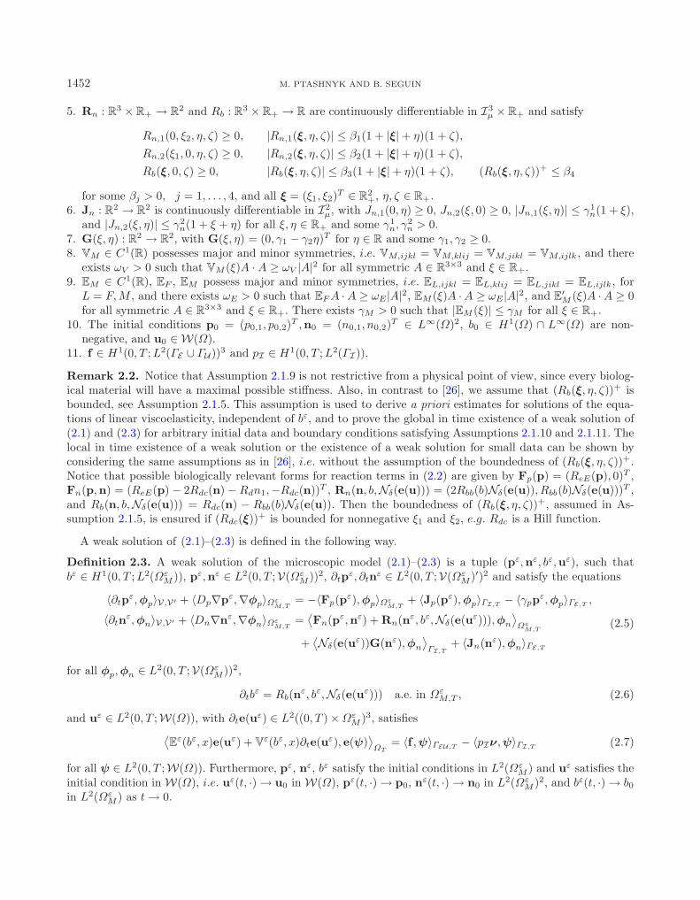
Remark 2.2. Notice that Assumption 2.1.9 is not restrictive from a physical point of view, since every biolog-ical material will have a maximal possible stiffness. Also, in contrast to [26], we assume that (Rb(ξ, η, ζ))+ isbounded, see Assumption 2.1.5. This assumption is used to derive a priori estimates for solutions of the equa-tions of linear viscoelasticity, independent of bε, and to prove the global in time existence of a weak solution of(2.1) and (2.3) for arbitrary initial data and boundary conditions satisfying Assumptions 2.1.10 and 2.1.11. Thelocal in time existence of a weak solution or the existence of a weak solution for small data can be shown byconsidering the same assumptions as in [26], i.e. without the assumption of the boundedness of (Rb(ξ, η, ζ))+.Notice that possible biologically relevant forms for reaction terms in (2.2) are given by Fp(p) = (ReE(p), 0)T ,Fn(p,n) = (ReE(p) − 2Rdc(n) −Rdn1,−Rdc(n))T , Rn(n, b,Nδ(e(u))) = (2Rbb(b)Nδ(e(u)), Rbb(b)Nδ(e(u)))T ,and Rb(n, b,Nδ(e(u))) = Rdc(n) − Rbb(b)Nδ(e(u)). Then the boundedness of (Rb(ξ, η, ζ))+, assumed in As-sumption 2.1.5, is ensured if (Rdc(ξ))+ is bounded for nonnegative ξ1 and ξ2, e.g. Rdc is a Hill function.

A weak solution of (2.1)–(2.3) is defined in the following way.

Definition 2.3. A weak solution of the microscopic model (2.1)–(2.3) is a tuple (pε,nε, bε,uε), such thatbε ∈ H1(0, T ;L2(Ωε

M )), pε,nε ∈ L2(0, T ;V(ΩεM ))2, ∂tpε, ∂tnε ∈ L2(0, T ;V(Ωε

M)′)2 and satisfy the equations

〈∂tpε,φp〉V,V′ + 〈Dp∇pε,∇φp〉ΩεM,T

= −〈Fp(pε),φp〉ΩεM,T

+ 〈Jp(pε),φp〉ΓI,T − 〈γppε,φp〉ΓE,T ,

〈∂tnε,φn〉V,V′ + 〈Dn∇nε,∇φn〉ΩεM,T

=⟨Fn(pε,nε) + Rn(nε, bε,Nδ(e(uε))),φn

⟩Ωε

M,T

+⟨Nδ(e(uε))G(nε),φn

⟩ΓI,T

+ 〈Jn(nε),φn〉ΓE,T

(2.5)

for all φp,φn ∈ L2(0, T ;V(ΩεM))2,

∂tbε = Rb(nε, bε,Nδ(e(uε))) a.e. in Ωε

M,T , (2.6)

and uε ∈ L2(0, T ;W(Ω)), with ∂te(uε) ∈ L2((0, T )×ΩεM )3, satisfies⟨

Eε(bε, x)e(uε) + V

ε(bε, x)∂te(uε), e(ψ)⟩

ΩT= 〈f ,ψ〉ΓEU,T − 〈pIν,ψ〉ΓI,T (2.7)

for all ψ ∈ L2(0, T ;W(Ω)). Furthermore, pε, nε, bε satisfy the initial conditions in L2(ΩεM ) and uε satisfies the

initial condition in W(Ω), i.e. uε(t, ·) → u0 in W(Ω), pε(t, ·) → p0, nε(t, ·) → n0 in L2(ΩεM )2, and bε(t, ·) → b0

in L2(ΩεM ) as t→ 0.


3. Main results

The main result of this paper is the derivation of the macroscopic equations for the microscopic viscoelasticmodel for plant cell wall biomechanics. The main difference between the homogenization results presented hereand those in [26] is due to the presence of a degenerate viscous term in the equations for the mechanicaldeformations of a cell wall. The fact that only the cell wall matrix is viscoelastic and the dependence of theviscosity tensor on the time variable, via the dependence on the cross-links density bε, make the multiscaleanalysis nonclassical and complex.

First we formulate the well-posedness result for the model (2.1)–(2.3).

Theorem 3.1. Under Assumption 2.1 there exists a unique weak solution of (2.1)–(2.3) satisfying the a prioriestimates

‖bε‖L∞(0,T ;L∞(ΩεM )) + ‖(∂tb

ε)+‖L∞(0,T ;L∞(ΩεM )) ≤ C1, (3.1)

where the constant C1 is independent of ε and δ,

‖uε‖L∞(0,T ;W(Ω)) + ‖∂te(uε)‖L2((0,T )×ΩεM) ≤ C2, (3.2)

where the constant C2 is independent of ε, and

‖pε‖L∞(0,T ;L∞(ΩεM )) + ‖∇pε‖L2(Ωε

M,T ) + ‖nε‖L∞(0,T ;L∞(ΩεM )) + ‖∇nε‖L2(Ωε

M,T ) ≤ C3,

‖∂tbε‖L∞(0,T ;L∞(Ωε

M )) ≤ C3,

‖θhpε − pε‖L2(ΩεM,T−h) + ‖θhnε − nε‖L2(Ωε

M,T−h) ≤ C3h1/4

(3.3)

for any h > 0, where θhv(t, x) = v(t + h, x) for (t, x) ∈ ΩεM,T−h, with h ∈ (0, T ), and the constant C3 is

independent of ε and h.

The proof of Theorem 3.1 is similar to the proof of the corresponding existence and uniqueness results in [26].Thus here we will only sketch the main ideas of the proof and emphasise the steps that are different from thoseof the proof in [26].

To formulate the macroscopic equations for the microscopic model (2.1)–(2.3), first we define the macroscopiccoefficients which will be obtained in the derivation of the limit equations. The macroscopic coefficients comingfrom the elasticity tensor are given by

Ehom,ijkl(b) = −∫

Y

[Eijkl(b, y) +

(E(b, y) ey(wij)

)kl

]dy,

Kijkl(t, s, b) = −∫

Y

(E(b(t+ s), y) ey(vij(t, s))

)kl

dy,(3.4)

and the macroscopic elasticity and viscosity tensors and the memory kernel read:

Ehom,ijkl(b) = Ehom,ijkl(b) +1|Y |

∫YM

(VM (b) ∂tey(wij)

)kl

dy,

Vhom,ijkl(b) =1|Y |

∫YM

[VM,ijkl(b) +

(VM (b) ey(χ

ijV

))

kl

]dy,

Kijkl(t, s, b) = Kijkl(t, s, b) +1|Y |

∫YM

(VM (b(t+ s)) ∂tey(vij(t, s))

)kl

dy,

(3.5)


where wij , χijV

, and vij , with i, j = 1, 2, 3, are solutions of the ‘unit cell’ problems

divy

(E(b, y)(ey(wij) + bij) + V(b, y)∂tey(wij)

)= 0 in YT ,

wij(0, x, y) = 0 in Y ,

divy

(VM (b)(ey(χij

V) + bij)

)= 0 in YM ,

VM (b)(ey(χijV

) + bij)ν = 0 on Γ ,∫Y

wijdy = 0,∫

YM

χijV

dy = 0, wij , χijV

Y -periodic,

(3.6)

where bjk = 12 (bj ⊗ bk + bk ⊗ bj), with {bj}1≤j≤3 being the canonical basis of R

3, and

divy

(E(b(t+ s, x), y)ey(vij) + V(b(t+ s, x), y)∂tey(vij)

)= 0 in YT−s,

vij(0, s, x, y) = χijV

(s, x, y) − wij(s, x, y) in Y ,∫Y

vijdy =∫

Y

χijV

dy, vij Y -periodic,

(3.7)

for x ∈ Ω and s ∈ [0, T ], where χijV

is an extension of χijV

from YM into Y . Here for a vector functionv = (v1, v2, v3)T we denote divyv = ∂y1v1 + ∂y2v2 and ey(v) is defined in the following way: ey(v)33 = 0,ey(v)3j = ey(v)j3 = 1

2∂yjv3 for j = 1, 2, and ey(v)ij = 12 (∂yivj + ∂yjvi) for i, j = 1, 2.

The macroscopic diffusion coefficients are defined by

Dlα,ij = −

∫YM

[Dl

α,ij + (Dlα∇yv

jα,l)i

]dy for i, j = 1, 2, 3, α = p, n, l = 1, 2, (3.8)

where ∇yvjα,l = (∂y1v

jα,l, ∂y2v

jα,l, 0)T and the functions vj

α,l are solutions of the ‘unit cell’ problems

divy(Dlα∇yv

jα,l) = 0 in YM , j = 1, 2, 3,

(Dlα∇yv

jα,l + Dl

αbj) · ν = 0 on Γ , vjα,l Y − periodic,

∫YM

vjα,l dy = 0,

(3.9)

where ∇y = (∂y1 , ∂y2)T , Dlα = (Dl

α,ik)i,k=1,2 and Dlα = (Dl

α,ik)i=1,2,k=1,2,3, with l = 1, 2 and α = p, n.Applying techniques of periodic homogenization we obtain the macroscopic equations for plant cell wall

biomechanics.

Theorem 3.2. A sequence of solutions of the microscopic model (2.1)–(2.3) converges to a solution of themacroscopic equations

∂tp = div(Dp∇p) − Fp(p) in ΩT ,

∂tn = div(Dn∇n) + Fn(p,n) + Rn(n, b,N effδ (e(u))) in ΩT ,

∂tb = Rb(n, b,N effδ (e(u))) in ΩT ,

(3.10)

together with the initial and boundary conditions

Dp∇pν = θ−1M Jp(p), Dn∇nν = θ−1

M G(n)N effδ (e(u)) on ΓI,T ,

Dp∇pν = −θ−1M γp p, Dn∇nν = θ−1

M Jn(n) on ΓE,T ,

Dp∇pν = 0, Dn∇nν = 0 on ΓU ,T ,

p, n a3-periodic in x3,

p(0) = p0, n(0) = n0, b(0) = b0 in Ω,

(3.11)


where θM = |YM |/|Y |, and the macroscopic equations of linear viscoelasticity

div(

Ehom(b)e(u) + Vhom(b)∂te(u) +∫ t

0

K(t− s, s, b)∂se(u) ds)

= 0 in ΩT ,(Ehom(b)e(u) + Vhom(b)∂te(u) +

∫ t

0

K(t− s, s, b)∂se(u) ds)ν = f on ΓEU ,T ,(

Ehom(b)e(u) + Vhom(b)∂te(u) +∫ t

0

K(t− s, s, b)∂se(u) ds)ν = −pIν on ΓI,T ,

u a3-periodic in x3,

u(0) = u0 in Ω.

(3.12)

Here

N effδ (e(u)) =

(−∫

Bδ(x)∩Ω

tr[Ehom(b)e(u) +

∫ t

0

K(t− s, s, b)∂se(u)ds]dx

)+

for (t, x) ∈ (0, T ) ×Ω. (3.13)

4. Existence of a unique weak solution of the microscopic problem (2.1)–(2.3).a priori estimates

In the derivation of a priori estimates for solutions of the microscopic problem (2.1)–(2.3) we shall usean extension of a function defined on a connected perforated domain Ωε

M to Ω. Applying classical extensionresults [2, 9, 15, 22], we obtain the following lemma.

Lemma 4.1. There exists an extension vε of vε from W 1,p(ΩεM ) into W 1,p(Ω), with 1 ≤ p <∞, such that

‖vε‖Lp(Ω) ≤ μ1‖vε‖Lp(ΩεM ) and ‖∇vε‖Lp(Ω) ≤ μ1‖∇vε‖Lp(Ωε

M ),

where the constant μ1 depends only on Y and YM , and YM ⊂ Y is connected.There exists an extension wε of wε from H1(Ωε

M )3 into H1(Ω)3 such that

‖wε‖Lp(Ω) ≤ μ2‖wε‖Lp(ΩεM ), ‖∇wε‖Lp(Ω) ≤ μ2‖∇wε‖Lp(Ωε

M ), ‖e(wε)‖Lp(Ω) ≤ μ2‖e(wε)‖Lp(ΩεM ),

where the constant μ2 does not depend on wε and ε.

Remark 4.2. Notice that the microfibrils do not intersect the boundaries ΓI , ΓU , and ΓE , and near the bound-aries ΓP = ∂Ω \ (ΓI ∪ΓE ∪ ΓU) it is sufficient to extend vε and wε by reflection in the directions normal to themicrofibrils and parallel to the boundary. Thus, classical extension results [2, 9, 15, 22, 25] apply to Ωε

M .In the sequel, we identify pε and nε with their extensions.

First we show the well-posedness and a priori estimates for equations (2.2) and (2.3) for a given uε ∈L∞(0, T ;W(Ω)). Next for a given bε we show the existence of a unique solution of the viscoelastic problem (2.1).Then using the fact that the estimates for bε can be obtained independently of uε and applying a fixed pointargument we show the well-posedness of the coupled system.

Lemma 4.3. Under Assumption 2.1 and for uε ∈ L∞(0, T ;W(Ω)) such that

‖uε‖L∞(0,T ;W(Ω)) ≤ C, (4.1)

where the constant C is independent of ε, there exists a unique weak solution (pε,nε, bε) of the microscopicproblem (2.2) and (2.3), with pε = (pε

1, pε2)

T and nε = (nε1, n

ε2)

T , satisfying

pεj(t, x) ≥ 0, nε

j(t, x) ≥ 0, bε(t, x) ≥ 0 for (t, x) ∈ (0, T )×ΩεM , j = 1, 2,

and the a priori estimates (3.1) and (3.3).


Proof. The proof of this lemma follows along the same lines as the proof of Theorem 3.1 in [26]. The onlydifference is in the derivation of the estimates for bε. Using the non-negativity of nε

1, nε2, b

ε, and Assumption 2.1.5we obtain from the equation for bε

0 ≤ bε(t, x) ≤ ‖b0‖L∞(Ω) + T ‖(Rb(nε, bε,Nδ(e(uε))))+‖L∞(0,T ;L∞(ΩεM )) ≤ C for (t, x) ∈ Ωε

M,T ,

(∂tbε(t, x))+ ≤ ‖(Rb(nε, bε,Nδ(e(uε))))+‖L∞(0,T ;L∞(Ωε

M )) ≤ β4 for (t, x) ∈ ΩεM,T .

(4.2)

Hence, the bounds for bε and (∂tbε)+ are independent of the bound for ‖uε‖L∞(0,T ;W(Ω)). This fact is important

for the derivation of a priori estimates for uε and for the fixed point argument in the proof of the existence ofa global weak solution for the coupled system.

Using the equation for bε, the definition of Nδ, and the estimates for ‖nε‖L∞(0,T ;L∞(ΩεM )), ‖bε‖L∞(0,T ;L∞(Ωε

M )),and ‖uε‖L∞(0,T ;W(Ω)) we obtain the estimate for ‖∂tb

ε‖L∞(0,T ;L∞(ΩεM )) uniformly in ε.

Similar to [26], integrating the equations for pε and nε over (t, t + h), with h ∈ (0, T ), and consideringφp = θhpε − pε and φn = θhnε − nε as test functions, respectively, we obtain the last estimate in (3.3). �

Next we prove the existence, uniqueness and a priori estimates for a solution of the viscoelastic equations fora given bε ∈ L∞(0, T ;L∞(Ωε

M )).

Lemma 4.4. Under Assumption 2.1 for a given bε ∈ L∞(0, T ;L∞(ΩεM )), satisfying

‖bε‖L∞(0,T ;L∞(ΩεM )) + ‖(∂tb

ε)+‖L∞(0,T ;L∞(ΩεM )) ≤ B, (4.3)

where the constant B is independent of ε, there exists a weak solution of the degenerate viscoelastic equa-tions (2.1) satisfying the a priori estimate (3.2).

Proof. Using the estimates for uε and ∂tuε, similar to those in (4.5), along with the positive definiteness of E

and V, and applying the Galerkin method, yield the existence of a weak solution of the problem (2.1).Since ∂te(uε) is only defined in Ωε

M , to derive a priori estimates we first consider an approximation of ∂tuε

∂tuε,ζ(t, x) =1ζ

∫ t

t−ζ

∂s1ζ

∫ s+ζ

s

uε(σ, x) dσ ds (4.4)

as a test function in (2.7), then integrate by parts in the elastic term and take the limit as ζ → 0. Using theassumptions on E and V, together with the non-negativity of bε, the boundedness of bε and (∂tb

ε)+, independentof ε and uε, and the trace and Korn inequalities, we obtain

ωE

2‖e(uε)(τ)‖2

L2(Ω) + ωV ‖∂te(uε)‖2L2(Ωε

M,τ ) ≤12〈(∂tb

ε)+E′M (bε)e(uε), e(uε)〉Ωε

M,τ+ C1‖e(u0)‖2

L2(Ω)

+〈f , ∂tuε〉ΓEU,τ − 〈pIν, ∂tuε〉ΓI,τ ≤ C2‖e(uε)‖2L2(Ωτ ) + σ‖e(uε)(τ)‖2

L2(Ω) + Cσ

[‖∂tf‖2

L2(ΓEU,τ )

+‖∂tpI‖2L2(ΓI,τ ) + ‖f(τ)‖2

L2(ΓEU ) + ‖pI(τ)‖2L2(ΓI) + ‖f(0)‖2

L2(ΓEU ) + ‖pI(0)‖2L2(ΓI)

]+ C3

for τ ∈ (0, T ]. Choosing σ sufficiently small and applying the Gronwall inequality imply

‖e(uε)‖L∞(0,T ;L2(Ω)) + ‖∂te(uε)‖L2(ΩεM,T ) ≤ C, (4.5)

with a constant C independent of ε. Then the second Korn inequality yields (3.2). �

Now applying a fixed point argument and using the results in Lemmas 4.3 and 4.4 we obtain the well-posednessof the coupled system (2.1)–(2.3).


Proof of Theorem 3.1. For a given uε ∈ L∞(0, T ;W(Ω)), with ‖uε‖L∞(0,T ;W(Ω)) ≤ C, Lemma 4.3 implies theexistence of a non-negative weak solution (pε,nε, bε) of the problem (2.2) and (2.3), where the estimates for‖bε‖L∞(0,T ;L∞(Ωε

M )) and ‖(∂tbε)+‖L∞(0,T ;L∞(Ωε

M )) are independent of uε and ε. Thus bε satisfies (4.3) fromLemma 4.4 and we have a solution uε of (2.1).

We define K : L∞(0, T ;W(Ω)) → L∞(0, T ;W(Ω)) by K(uε) = uε, where uε is a solution of (2.1) for bε

given as a solution of (2.2) and (2.3) with uε instead of uε, and show that for sufficiently small T ∈ (0, T ], theoperator K : L∞(0, T ;W(Ω)) → L∞(0, T ;W(Ω)) is a contraction, i.e. there is a γ ∈ (0, 1) such that

‖K(uε,1) −K(uε,2)‖L∞(0,T ;W(Ω)) ≤ γ‖uε,1 − uε,2‖L∞(0,T ;W(Ω)) for uε,1, uε,2 ∈ L∞(0, T ;W(Ω)).

Considering the difference of equation (2.7) for (uε,1, bε,1) and (uε,2, bε,2), and taking the approximation of∂t(uε,1 − uε,2), defined as in (4.4), as a test function, in the same way as in the proof of Lemma 4.4, yield

12〈Eε(bε,1, x)e(uε,1(τ) − uε,2(τ)), e(uε,1(τ) − uε,2(τ))〉Ω + 〈Vε(bε,1, x)∂te(uε,1 − uε,2), ∂te(uε,1 − uε,2)〉Ωτ

−12〈∂tb

ε,1E′M (bε,1)e(uε,1 − uε,2), e(uε,1 − uε,2)〉Ωε

M,τ= 〈(EM (bε,2) − EM (bε,1))e(uε,2), ∂te(uε,1 − uε,2)〉Ωε

M,τ

+〈(VM (bε,2) − VM (bε,1))∂te(uε,2), ∂te(uε,1 − uε,2)〉ΩεM,τ

for τ ∈ (0, T ]. By the assumptions on Eε and V

ε and the boundedness of bε,1 and bε,2, we have

‖e(uε,1(τ)) − e(uε,2(τ))‖2L2(Ω) ≤ C1‖(∂tb

ε,1)+‖L∞(0,T ;L∞(ΩεM ))

∫ τ

0

‖e(uε,1 − uε,2)‖2L2(Ωε

M )dτ

+ C2‖e(uε,2)‖2H1(0,T ;L2(Ωε

M ))‖bε,1 − bε,2‖2L∞(0,τ ;L∞(Ωε

M )).

Applying the Gronwall inequality and the estimates for (∂tbε,1)+ and e(uε,2) implies

‖e(uε,1) − e(uε,2)‖2L∞(0,T ;L2(Ω))

≤ C3‖bε,1 − bε,2‖2L∞(0,T ;L∞(Ωε

M ))(4.6)

for T ∈ (0, T ].Now we shall estimate ‖bε,1 − bε,2‖2

L∞(0,T ;L∞(ΩεM ))

in terms of T‖e(uε,1) − e(uε,2)‖2L∞(0,T ;L2(Ω))

for any

T ∈ (0, T ]. Following the same calculations as in [26], we first consider equation (2.5)2 for nε,1 and nε,2, takeφn = (|nε

1|q−2nε1, |nε

2|q−2nε2)

T , where nεj = nε,1

j − nε,2j with j = 1, 2 and q ≥ 2, and subtract the resulting

equations. Using the definition of Nδ, the assumptions on G and Jn, and the trace inequality, the boundaryterms are estimated in the following way⟨

Nδ(e(uε,1))[G(nε,1) − G(nε,2)

], (|nε

1|q−2nε1, |nε

2|q−2nε2)

T⟩

ΓI≤ 0,⟨

Jn(nε,1) − Jn(nε,2), (|nε1|q−2nε

1, |nε2|q−2nε

2)T⟩

ΓE≤ Cσq ‖nε,1 − nε,2‖q

Lq(ΩεM )

+ σ(q − 1)/q2 ‖∇|nε,1 − nε,2|q2 ‖2

L2(ΩεM )

and ∣∣∣⟨G(nε,2)[Nδ(e(uε,1)) −Nδ(e(uε,2))

], (|nε

1|q−2nε1, |nε

2|q−2nε2)

T⟩

ΓI

∣∣∣ ≤ Cσ(q − 1)‖nε,12 − nε,2

2 ‖qLq(Ωε

M )

+σ(q − 1)/q2‖∇|nε,12 − nε,2

2 |q2 ‖2

L2(ΩεM ) + (C/q)‖Nδ(e(uε,1)) −Nδ(e(uε,2))‖q

Lq(Ω),

with an arbitrary σ > 0. Using the assumptions on Fn and Rn and the uniform boundedness of pε, nε,j , andbε,j , with j = 1, 2, we obtain

〈Fn(pε,nε,1) − Fn(pε,nε,2), (|nε1|q−2nε

1, |nε2|q−2nε

2)T 〉Ωε

M≤ C1‖nε,1 − nε,2‖q

Lq(ΩεM ),

〈Rn(nε,1, bε,1,Nδ(e(uε,1))) − Rn(nε,2, bε,2,Nδ(e(uε,2))), (|nε1|q−2nε

1, |nε2|q−2nε

2)T 〉Ωε

M≤ C2

[‖Nδ(e(uε,1))‖L∞(Ω)

+ ‖Nδ(e(uε,2))‖L∞(Ω) + 1][‖nε,1 − nε,2‖q

Lq(ΩεM ) +

1q‖bε,1 − bε,2‖q

Lq(ΩεM ) +

1q‖Nδ(e(uε,1)) −Nδ(e(uε,2))‖q

Lq(Ω)

].


Then, the Gagliardo–Nirenberg inequality applied to |nε,1 − nε,2|q/2, the definition of Nδ(e(uε,j)), the a prioriestimates for uε,1 and uε,2, together with the estimate

‖Nδ(e(uε,1)) −Nδ(e(uε,2))‖qLq(Ω) ≤ Cqδ−

3q2[‖e(uε,1) − e(uε,2)‖q

L2(Ω) + ‖bε,1 − bε,2‖qLq(Ωε

M )

],

ensure∂t‖nε,1 − nε,2‖q

Lq(ΩεM ) + 2

q − 1q

‖∇|nε,1 − nε,2|q2 ‖2

L2(ΩεM ) ≤ C

[q5‖nε,1 − nε,2‖q

Lq/2(ΩεM )

+(Cqδ + 1)

[‖bε,1 − bε,2‖q

Lq(ΩεM ) + ‖e(uε,1) − e(uε,2)‖q

L2(Ω)

]].

Here we use the notation |nε,1 − nε,2|α = |nε,11 − nε,2

1 |α + |nε,12 − nε,2

2 |α. Considering iterations in q as in ([3],Lem. 3.2) with q = 2κ and κ = 2, 3, . . . , we obtain

‖nε,1(τ) − nε,2(τ)‖qLq(Ωε

M ) ≤ Cqδ 210q22(q−1)

[‖e(uε,1) − e(uε,2)‖q

L∞(0,τ ;L2(Ω)) + ‖bε,1 − bε,2‖qL∞(0,τ ;Lq(Ωε

M ))

]for τ ∈ (0, T ] and Cδ ≥ 1. Taking the qth root, and considering q → ∞ yield

‖nε,1 − nε,2‖L∞(0,τ ;L∞(ΩεM )) ≤ Cδ

[‖e(uε,1) − e(uε,2)‖L∞(0,τ ;L2(Ω)) + ‖bε,1 − bε,2‖L∞(0,τ ;L∞(Ωε

M ))

]. (4.7)

Considering the difference of equations (2.6) for bε,1 and bε,2, multiplying by bε,1−bε,2, and using the assumptionson Rb and estimate (4.7) we obtain the following estimate for bε,1 − bε,2

‖bε,1 − bε,2‖2L∞(0,τ ;L∞(Ωε

M )) ≤ Cδτ[‖e(uε,1) − e(uε,2)‖2

L∞(0,τ ;L2(Ω)) + ‖bε,1 − bε,2‖2L∞(0,τ ;L∞(Ωε

M ))

]for τ ∈ (0, T ]. Then, the iteration over time intervals of length 1/(2Cδ) ensures

‖bε,1 − bε,2‖2L∞(0,T ;L∞(Ωε

M ))≤ CT‖e(uε,1 − uε,2)‖2

L∞(0,T ;L2(Ω))(4.8)

for T ∈ (0, T ]. Thus, combining (4.6) and (4.8) we have that the operator K : L∞(0, T ;W(Ω)) →L∞(0, T ;W(Ω)), defined by K(uε) = uε, where uε is a weak solution of (2.1), is a contraction for sufficientlysmall T , where T depends on the coefficients in the microscopic equations and is independent of (pε,nε, bε,uε)and uε. Hence, using the Banach fixed point theorem and iterating over time intervals, we obtain the existenceof a unique weak solution of the microscopic problem (2.1)–(2.3). �

Remark 4.5. Without the assumption that (Rb(nε, bε,Nδ(e(uε))))+ is bounded we can prove a local in timeexistence of a weak solution of the microscopic problem using a cut-off method. First we assume that

(Rb(nε, bε,Nδ(e(uε))))+ ≤ β3(1 + ‖nε‖L∞(0,T ;L∞(ΩεM )) + ‖bε‖L∞(0,T ;L∞(Ωε

M )))(1 + Cδ‖uε‖L∞(0,T ;W(Ω))) ≤ β.

Then we have that bε satisfies (4.3) and obtain ‖uε‖L∞(0,T ;W(Ω)) ≤ C1eT (B(β)+C2). The derivation of theestimates for nε and bε yields

‖bε‖L∞(0,T ;L∞(ΩεM )) + ‖nε‖L∞(0,T ;L∞(Ωε

M )) ≤ C(2C1T (1+‖uε‖L∞(0,T ;W(Ω))) + 1) ≤ C(2C2T (eT(B(β)+C3)+1) + 1).

Then for sufficient small T and an appropriate choice of β we obtain that (Rb(nε, bε,Nδ(e(uε))))+ ≤ β.

5. Derivation of the macroscopic equations of the problem (2.1)–(2.3): Proof

of Theorem 3.2

Due to the fact that the viscous term is positive definite in the cell wall matrix and is zero for the cell wallmicrofibrils, to derive macroscopic equations for the microscopic problem (2.1)–(2.3) we consider a perturbedproblem by adding the inertial term ϑ∂2

t uε,ϑχΩε

M, where ϑ > 0 is a small perturbation parameter,

ϑχΩεM∂2

t uε,ϑ = div

(E

ε(bε,ϑ, x) e(uε,ϑ) + Vε(bε,ϑ, x) ∂te(uε,ϑ)

)in ΩT , (5.1)


and the additional initial condition∂tuε,ϑ(0, x) = 0 in Ω. (5.2)

We split the proof of Theorem 3.2 into three steps. First we derive the macroscopic equations for the perturbedsystem. Then letting the perturbation parameter ϑ go to zero we obtain the macroscopic equations (3.10)–(3.12).To verify that (3.10)–(3.12) are the macroscopic equations for the microscopic problem (2.1)–(2.3), we showthat the macroscopic two-scale problem is the same for the original microscopic model and for the perturbedmicroscopic model when the perturbation parameter ϑ→ 0.

Lemma 5.1. There exists a unique weak solution (pε,ϑ,nε,ϑ, bε,ϑ,uε,ϑ) of the perturbed microscopic problem(2.2), (2.3) and (5.1), together with the initial and boundary conditions in (2.1) and (5.2), satisfying the a prioriestimates

ϑ12 ‖∂tuε,ϑ‖L∞(0,T ;L2(Ωε

M )) + ‖uε,ϑ‖L∞(0,T ;W(Ω)) + ‖∂te(uε,ϑ)‖L2(ΩεM,T ) ≤ C, (5.3)

and‖pε,ϑ‖L∞(0,T ;L∞(Ωε

M )) + ‖∇pε,ϑ‖L2(ΩεM,T ) + ‖nε,ϑ‖L∞(0,T ;L∞(Ωε

M )) + ‖∇nε,ϑ‖L2(ΩεM,T ) ≤ C,

‖bε,ϑ‖L∞(0,T ;L∞(ΩεM )) + ‖∂tb

ε,ϑ‖L∞(0,T ;L∞(ΩεM )) ≤ C,

‖θhpε,ϑ − pε,ϑ‖L2(ΩεM,T−h) + ‖θhnε,ϑ − nε,ϑ‖L2(Ωε

M,T−h) ≤ Ch1/4,

(5.4)

where θhv(t, x) = v(t+h, x) for (t, x) ∈ ΩεM,T−h and h ∈ (0, T ), and the constant C is independent of ε, ϑ, and

h.

Proof. For a given uε,ϑ ∈ L∞(0, T ;W(Ω)), with ‖uε,ϑ‖L∞(0,T ;W(Ω)) ≤ C, in the same way as in Lemma 4.3 weobtain the existence of a unique solution of the problem (2.2) and (2.3), satisfying the a priori estimates (5.4).Notice that the estimates for bε,ϑ and (∂tb

ε,ϑ)+ are independent of uε,ϑ, ε, and ϑ.Then for bε,ϑ ∈ L∞(0, T ;L∞(Ωε

M )), with ‖bε,ϑ‖L∞(0,T ;L∞(ΩεM )) ≤ C and ‖(∂tb

ε,ϑ)+‖L∞(0,T ;L∞(ΩεM )) ≤ C,

similar to Lemma 4.4, we obtain the existence of a weak solution of the perturbed equations (5.1) with initialand boundary conditions in (2.1) and (5.2), satisfying estimate (5.3).

Similar to the proof of Theorem 3.1, considering the difference of equation (5.1) for (uε,ϑ,j , bε,ϑ,j), withj = 1, 2, and taking the approximation of ∂t(uε,ϑ,1 − uε,ϑ,2), as in (4.4), as a test function yield

12ϑ‖∂tuε,ϑ,1(τ) − ∂tuε,ϑ,2(τ)‖2

L2(ΩεM ) +

12⟨E

ε(bε,ϑ,1, x)e(uε,ϑ,1 − uε,ϑ,2)(τ), e(uε,ϑ,1 − uε,ϑ,2)(τ)⟩

Ω

−12⟨∂tb

εE′M (bε,ϑ,1)e(uε,ϑ,1 − uε,ϑ,2), e(uε,ϑ,1 − uε,ϑ,2)

⟩Ωε

M,τ

+⟨V

ε(bε,ϑ,1, x)∂te(uε,ϑ,1 − uε,ϑ,2), ∂te(uε,ϑ,1 − uε,ϑ,2)⟩

Ωτ

=⟨(EM (bε,ϑ,2) − EM (bε,ϑ,1))e(uε,ϑ,2) + (VM (bε,ϑ,2) − VM (bε,ϑ,1))∂te(uε,ϑ,2), ∂te(uε,ϑ,1 − uε,ϑ,2)

⟩Ωε

M,τ

for τ ∈ (0, T ]. By the assumptions on Eε and V

ε, using the estimates for (∂tbε,ϑ,1)+, e(uε,ϑ,2), and ∂te(uε,ϑ,2),

together with the boundedness of bε,ϑ,1 and bε,ϑ,2, and applying the Gronwall inequality we obtain

‖e(uε,ϑ,1) − e(uε,ϑ,2)‖2L∞(0,T ;L2(Ω))

≤ C‖bε,ϑ,1 − bε,ϑ,2‖2L∞(0,T ;L∞(Ωε

M ))(5.5)

for all T ∈ (0, T ]. Then, using the estimates (4.8) and (5.5), together with the a priori estimates for uε,ϑ, pε,ϑ,nε,ϑ, and bε,ϑ, in the same way as in the proof of Theorem 3.1 we obtain the existence of a unique weak solutionof the perturbed problem (2.2) and (5.1), with the initial and boundary conditions in (2.1), (2.3), and (5.2).�

To verify a relation between the perturbed and original microscopic problems, we show that a sequence ofweak solutions of the perturbed problem (2.2), (2.3), and (5.1), with initial and boundary conditions in (2.1)and (5.2), converges as ϑ→ 0 to a weak solution of the original problem (2.1)–(2.3).


Lemma 5.2. A sequence of solutions {pε,ϑ,nε,ϑ, bε,ϑ,uε,ϑ} of the problem (2.2), (2.3) and (5.1), together withthe initial and boundary conditions in (2.1) and (5.2), converges as ϑ → 0 to a unique solution (pε,nε, bε,uε)of the microscopic problem (2.1)–(2.3).

Proof. Estimates (5.3) and (5.4) ensure that there exist functions pε,nε ∈ L2(0, T ;V(ΩεM))2 ∩

L∞(0, T ;L∞(ΩεM ))2, bε ∈ W 1,∞(0, T ;L∞(Ωε

M )), uε ∈ L2(0, T ;W(Ω)), Λε ∈ L2(ΩεM,T )3×3, and ηε ∈

L∞(0, T ;L2(ΩεM ))3 such that, up to a subsequence,

pε,ϑ ⇀ pε, nε,ϑ ⇀ nε weakly in L2(0, T ;H1(ΩεM ))2,

pε,ϑ → pε, nε,ϑ → nε strongly in L2(ΩεM,T )2,

bε,ϑ ⇀ bε, ∂tbε,ϑ ⇀ ∂tb

ε weakly in Lp(ΩεM,T ), p ∈ [2,∞),

uε,ϑ ⇀ uε weakly in L2(0, T ;W(Ω)),

∂te(uε,ϑ) ⇀ Λε weakly in L2(ΩεM,T )3×3,

ϑ1/2∂tuε,ϑ ⇀ ηε weakly in L2(ΩεM,T )3,

(5.6)

as ϑ → 0. Using the weak convergence of e(uε,ϑ) we obtain that Λε = ∂te(uε) a.e. in L2(ΩεM,T ). Considering

the equation for bε,ϑ at (t, x) and (t, x+ hj) and using the assumptions on Rb yield

‖bε,ϑ(τ, · + hj) − bε,ϑ(τ, ·)‖2L2(Ωε

M,h) ≤ ‖b0(· + hj) − b0(·)‖2L2(Ωε

M,h) + C1

∫ τ

0

‖bε,ϑ(t, · + hj) − bε,ϑ(t, ·)‖2L2(Ωε

M,h)dt

+ C2

∫ τ

0

[‖nε,ϑ(t, · + hj) − nε,ϑ(t, ·)‖2

L2(ΩεM,h) + δ−6

∥∥∥∫Bδ,h(x)∩Ω

tr(E

ε(bε,ϑ, x) e(uε,ϑ(t, x)))

dx∥∥∥2

L2(ΩεM,h)

]dt

for τ ∈ (0, T ], where hj = hbj , with {bj}j=1,2,3 being the canonical basis in R3 and h > 0, Ωε

M,h = {x ∈Ωε

M | dist(x, ∂ΩεM ) > 2h}, Bδ,h(x) =

[Bδ(x + hj) \ Bδ(x)

]∪[Bδ(x) \ Bδ(x + hj)

], and the constants C1, C2

are independent of ϑ and h. Using the regularity of b0, the estimates for ∇nε,ϑ and e(uε,ϑ), the boundednessof bε,ϑ, and the fact that |Bδ,h(x) ∩Ω| ≤ Cδ2h for all x ∈ Ω, and applying the Gronwall inequality we obtain

supt∈(0,T )

‖bε,ϑ(t, · + hj) − bε,ϑ(t, ·)‖2L2(Ωε

M,h) ≤ Ch. (5.7)

The estimate for ∂tbε,ϑ ensures

‖bε,ϑ(· + h, ·) − bε,ϑ(·, ·)‖2L2((0,T−h)×Ωε

M ) ≤ C1h2‖∂tb

ε,ϑ‖2L2(Ωε

M,T ) ≤ C2h2, (5.8)

where C2 is independent of ϑ and h. Combining (5.7) and (5.8), using the uniform boundedness of bε,ϑ, andapplying the Kolmogorov compactness theorem, see e.g. [5,20], yield the strong convergence of bε,ϑ in L2(Ωε

M,T )as ϑ → 0. Using arguments similar to those in the proof of Theorem 5.4 we obtain

‖θhe(uε,ϑ) − e(uε,ϑ)‖2L2((0,T−h)×Ω) ≤ Ch1/2,

‖e(uε,ϑ)‖2L2((T−h,T )×Ω) ≤ Ch,

(5.9)

with a constant C independent of ϑ and h. The last estimates, together with the strong convergence of bε,ϑ, thecontinuity of EM , and Lebesgue’s dominated convergence theorem, ensure the following strong convergences∫

Ω

E(bε,ϑ, x/ε)e(uε,ϑ)dx→∫

Ω

E(bε, x/ε)e(uε)dx in L2(0, T ),∫Bδ(x)∩Ω

E(bε,ϑ, x/ε)e(uε,ϑ)dx→∫

Bδ(x)∩Ω

E(bε, x/ε)e(uε)dx in L2(ΩT ) and L2(ΓI,T ),


as ϑ → 0. Hence we can pass to the limit as ϑ → 0 in the weak formulation of equations (2.2) and (5.1), withthe initial and boundary conditions in (2.1), (2.3), and (5.2), and obtain that the limit functions (pε,nε, bε,uε)satisfy the microscopic problem (2.1)–(2.3). The uniqueness of a weak solution of (2.1)–(2.3) ensures the con-vergence of the whole sequence of weak solutions of the perturbed microscopic problem. �

Next we consider the convergence of a sequence of solutions {pε,ϑ,nε,ϑ, bε,ϑ,uε,ϑ} of the perturbed microscopicproblem as ε→ 0.

Lemma 5.3. There exist functions pϑ,nϑ ∈ L2(0, T ;V(Ω))2 ∩ L∞(0, T ;L∞(Ω))2, pϑ, nϑ ∈L2(ΩT ;H1

per(Y )/R)2 and bϑ ∈ W 1,∞(0, T ;L∞(Ω)), uϑ ∈ H1(0, T ;W(Ω)), uϑ ∈ L2(ΩT ;H1per(Y )/R)3,

∂tuϑ ∈ L2(ΩT ;H1per(YM )/R)3 such that for a subsequence of solutions (pε,ϑ,nε,ϑ, bε,ϑ,uε,ϑ) of the perturbed

microscopic problem (2.2) and (5.1), with initial and boundary conditions in (2.1), (2.3) and (5.2), (denotedagain by (pε,ϑ,nε,ϑ, bε,ϑ,uε,ϑ)) we have the following convergence results:

pε,ϑ ⇀ pϑ, nε,ϑ ⇀ nϑ weakly in L2(0, T ;H1(Ω))2,

pε,ϑ → pϑ, nε,ϑ → nϑ strongly in L2(ΩT )2,

∇pε,ϑ ⇀ ∇pϑ + ∇ypϑ, ∇nε,ϑ ⇀ ∇nϑ + ∇ynϑ two-scale,

bε,ϑ ⇀ bϑ, ∂tbε,ϑ ⇀ ∂tb

ϑ two-scale,

T ∗ε (bε,ϑ) → bϑ strongly in L2(ΩT × YM ),

uε,ϑ ⇀ uϑ weakly in L2(0, T ;W(Ω)),

∇uε,ϑ ⇀ ∇uϑ + ∇yuϑ two-scale,

∂tuε,ϑ ⇀ ∂tuϑ weakly in L2(ΩT )3 and two-scale,

χΩεM∇∂tuε,ϑ ⇀ χYM

(∇∂tuϑ + ∇y∂tuϑ) two-scale,

(5.10)

as ε→ 0, where ∂tuε,ϑ and ∇∂tuε,ϑ are extended by zero from ΩεM into Ω and ∇y∂tuϑ is extended by zero from

YM into Y .

Here T ∗ε : Lp(Ωε

M,T ) → Lp(ΩT × YM ) is the unfolding operator defined as T ∗ε (φ)(t, x, y) = φ(t, ε[x/ε]YM

+εy, x3) for (t, x) ∈ ΩT and y ∈ YM , where x = (x1, x2) and [x/ε]YM

is the unique integer combination of theperiods such that x/ε− [x/ε]YM

∈ YM , see e.g. [8].

Proof. The a priori estimates in (5.4) imply the weak and two-scale convergences of pε,ϑ, nε,ϑ, bε,ϑ, and ∂tbε,ϑ.

Using the estimates for θhpε,ϑ − pε,ϑ, θhnε,ϑ − nε,ϑ, ∇nε,ϑ, and ∇pε,ϑ in (5.4), together with the propertiesof the extension of nε,ϑ and pε,ϑ from Ωε

M into Ω, see Lemma 4.1, and applying the Kolmogorov theorem, seee.g. [5, 20], we obtain the strong convergence of nε,ϑ and pε,ϑ in L2(ΩT ).

In the same way as in [26] we show the strong convergence T ∗ε (bε,ϑ) → bϑ in L2(ΩT × YM ) as ε → 0. Here

we present only a sketch of the calculations. Using the extension of nε,ϑ from ΩεM into Ω, see Lemma 4.1, we

define the extension of bε,ϑ from ΩεM into Ω as a solution of the ordinary differential equation

∂tbε,ϑ = Rb(nε,ϑ, bε,ϑ,Nδ(e(uε,ϑ))) in (0, T )×Ω,

bε,ϑ(0) = b0 in Ω.(5.11)

The construction of the extension for nε,ϑ and the uniform boundedness of nε,ϑ1 and nε,ϑ

2 in ΩεM,T , see (5.4),

ensure‖nε,ϑ‖L∞(0,T ;L∞(Ω)) ≤ C1‖nε,ϑ‖L∞(0,T ;L∞(Ωε

M )) ≤ C,

with the constant C independent of ε and ϑ. Notice that we identify nε,ϑ with its extension. Hence from (5.11),using estimate (5.3) for uε,ϑ, we obtain the boundedness of bε,ϑ and ∂tb

ε,ϑ. We show the strong convergence of bε,ϑ


using arguments similar to those found in the proof of Lemma 5.2 by applying the Kolmogorov theorem [5,20].Considering equation (5.11) at (t, x + hj) and (t, x), for j = 1, 2, 3, taking bε,ϑ(t, x + hj) − bε,ϑ(t, x) as a testfunction and using the Lipschitz continuity of Rb yield

‖bε,ϑ(τ, · + hj) − bε,ϑ(τ, ·)‖2L2(Ω2h) ≤ ‖b0(· + hj) − b0(·)‖2

L2(Ω2h) + C1

∫ τ

0

‖bε,ϑ(t, · + hj) − bε,ϑ(t, ·)‖2L2(Ω2h)dt

+ C2

∫ τ

0

(‖nε,ϑ(t, · + hj) − nε,ϑ(t, ·)‖2

L2(Ω2h) + δ−6∥∥∥∫

Bδ,h(x)∩Ω

tr Eε(bε,ϑ, x)e(uε,ϑ(t, x))dx

∥∥∥2

L2(Ω2h)

)dt

for τ ∈ (0, T ], where Ω2h = {x ∈ Ω | dist(x, ∂Ω) > 2h}, Bδ,h(x) is defined as in Lemma 5.2 with |Bδ,h(x)∩Ω| ≤Cδ2h for all x ∈ Ω, and the constants C1, C2 are independent of ε, ϑ, and h. Using the regularity of the initialcondition b0 ∈ H1(Ω) and the a priori estimates for e(uε,ϑ) and ∇nε,ϑ, and applying the Gronwall inequalitywe obtain

supt∈(0,T )

‖bε,ϑ(t, · + hj) − bε,ϑ(t, ·)‖2L2(Ω2h) ≤ Cδh. (5.12)

Extending bε,ϑ by zero from ΩT into R+ × R3 and using the uniform boundedness of bε,ϑ imply

‖bε,ϑ‖2L∞(0,T ;L2(Ω3h))

+ ‖bε,ϑ‖2L2((T−2h,T+2h)×Ω) ≤ Ch, (5.13)

where Ω3h = {x ∈ R3 | dist(x, ∂Ω) < 3h} and the constant C is independent of ε, ϑ, and h. The estimate for

∂tbε,ϑ ensures that

‖bε,ϑ(· + h, ·) − bε,ϑ(·, ·)‖2L2((0,T−h)×Ω) ≤ C1h

2‖∂tbε,ϑ‖2

L2(ΩT ) ≤ C2h2, (5.14)

where C1 and C2 are independent of ε, ϑ, and h. Combining (5.12)–(5.14) and applying the Kolmogorov theoremyield the strong convergence of bε,ϑ to bϑ in L2(ΩT ) as ε → 0. The definition of two-scale convergence impliesthat bϑ = bϑ and, hence, the two-scale limit of bε,ϑ is independent of y. Then using the properties of theunfolding operator, see e.g. [7, 8], we obtain the strong convergence of T ∗

ε (bε,ϑ).Considering an extension ∂tuε,ϑ of ∂tuε,ϑ from Ωε

M into Ω, see Lemma 4.1, and applying the Korn inequality,see e.g. [22], yield

‖∂tuε,ϑ‖L2(0,T ;H1(ΩεM )) ≤ ‖∂tuε,ϑ‖L2(0,T ;H1(Ω)) ≤ C1

[‖∂tuε,ϑ‖L2(ΩT ) + ‖e(∂tuε,ϑ)‖L2(ΩT )

]≤ C2

[‖∂tuε,ϑ‖L2(Ωε

M,T ) + ‖e(∂tuε,ϑ)‖L2(ΩεM,T )

]≤ C3(1 + ϑ−

12 ),

(5.15)

where the constant C3 is independent of ε and ϑ.The estimates (5.3) and (5.15) ensure the existence of functions uϑ ∈ L2(0, T ;W(Ω)), uϑ ∈

L2(ΩT ;H1per(Y )/R)3, ξϑ ∈ L2(0, T ;H1(Ω))3, and ξ

ϑ ∈ L2(ΩT ;H1per(YM )/R)3 such that

uε,ϑ ⇀ uϑ, ∇uε,ϑ ⇀ ∇uϑ + ∇yuϑ two-scale,

χΩεM∂tuε,ϑ ⇀ χYM

ξϑ, χΩεM∇∂tuε,ϑ ⇀ χYM

(∇ξϑ + ∇y ξϑ) two-scale,

as ε→ 0, see e.g. [4]. Considering the two-scale convergence of uε,ϑ and ∂tuε,ϑ, we obtain

|YM ||Y |

〈ξϑ, φ〉ΩT = limε→0

〈∂tuε,ϑ, φ〉ΩεM,T

= − limε→0

〈uε,ϑ, ∂tφ〉ΩεM,T

= −|YM ||Y |

〈uϑ, ∂tφ〉ΩT


for all φ ∈ C∞0 (ΩT ). Hence, ∂tuϑ ∈ L2(ΩT )3 and ξϑ = ∂tuϑ a.e. in ΩT . Thus ∂tuϑ ∈ L2(0, T ;W(Ω)). The

two-scale convergence of ∇uε,ϑ and ∂t∇uε,ϑ implies

|Y |−1〈∂t∇uϑ + ∇y ξϑ, φ〉ΩT ×YM

= limε→0

〈∂t∇uε,ϑ, φ〉ΩεM,T

= − limε→0

〈∇uε,ϑ, ∂tφ〉ΩεM,T

= −|Y |−1〈∇uϑ + ∇yuϑ, ∂tφ〉ΩT ×YM

for all φ ∈ C∞0 (ΩT ;C∞

per(Y )). Thus, ∂t∇yuϑ ∈ L2(ΩT ×YM )3×3 and ∇y ξϑ

= ∂t∇yuϑ a.e. in ΩT ×YM . Therefore,uϑ ∈ H1(0, T ;W(Ω)), ∂tuϑ ∈ L2(ΩT ;H1

per(YM )/R)3 and χΩεM∂te(uε,ϑ) ⇀ χYM

(∂te(uϑ) + ∂tey(uϑ)

)two-scale.

�

To derive macroscopic equations for the microscopic problem (2.1)–(2.3), we first derive the macroscopicequations for the perturbed system (2.2) and (5.1), with the initial and boundary conditions in (2.1), (2.3) and(5.2). Then letting the perturbation parameter go to zero we derive the macroscopic equations (3.10)–(3.12). Byshowing that the macroscopic two-scale problem is the same for the original microscopic equations (2.1)–(2.3)and for the perturbed microscopic problem as the perturbation parameter ϑ goes to zero, we conclude that(3.10)–(3.12) are the macroscopic equations for (2.1)–(2.3).

Theorem 5.4. A sequence of solutions (pε,ϑ,nε,ϑ, bε,ϑ,uε,ϑ), of the perturbed microscopic equations (2.2) and(5.1), with the initial and boundary conditions in (2.1), (2.3) and (5.2), converges, as ε → 0, to a solution(pϑ,nϑ, bϑ,uϑ) of the perturbed macroscopic problem

ϑ∂2t u

ϑ − div(

Eϑhom(bϑ) e(uϑ) + V

ϑhom(bϑ) ∂te(uϑ) +

∫ t

0

Kϑ(t− s, s, bϑ) ∂se(uϑ) ds

)= 0 in ΩT ,(



∫ t

0


)ν = f on ΓEU ,T ,(



∫ t

0


)ν = −pIν on ΓI,T ,

uϑ a3-periodic in x3,

uϑ(0) = u0, ∂tuϑ(0) = 0 in Ω,

(5.16)

and∂tpϑ = div(Dp∇pϑ) − Fp(pϑ) in ΩT ,

∂tnϑ = div(Dn∇nϑ) + Fn(pϑ,nϑ) + Rn(nϑ, bϑ,N effδ (e(uϑ))) in ΩT ,

∂tbϑ = Rb(nϑ, bϑ,N eff

δ (e(uϑ))) in ΩT ,

(5.17)

together with the initial and boundary conditions

Dp∇pϑ ν = θ−1M Jp(pϑ), Dn∇nϑ ν = θ−1

M G(nϑ)N effδ (e(uϑ)) on ΓI,T ,

Dp∇pϑ ν = −θ−1M γp pϑ, Dn∇nϑ ν = θ−1

M Jn(nϑ) on ΓE,T ,

Dp∇pϑ ν = 0, Dn∇nϑ ν = 0 on ΓU ,T ,

pϑ, nϑ a3-periodic in x3,

pϑ(0) = p0, nϑ(0) = n0, b(0) = b0 in Ω,

(5.18)

where Eϑhom, V

ϑhom, and K

ϑ are defined as in (3.4) and (3.5), with bϑ, wijϑ , χij

V,ϑ, and vijϑ instead of b, wij , χij

V,

and vij , where wijϑ , χij

V,ϑ, and vijϑ are solutions of the ‘unit cell’ problems (3.6) and (3.7) with bϑ instead of b,

for i, j = 1, 2, 3. The macroscopic diffusion matrices Dlα, with α = n, p and l = 1, 2, are defined as in (3.8) and

N effδ is defined as in (3.13) with bϑ and uϑ instead of b and u.


Proof. To pass to the limit in the equations for nε,ϑ and bε,ϑ, we shall first prove the strong convergence of∫Ω E(bϑ, x/ε) e(uε,ϑ)dx in L2(0, T ), as ε→ 0.Considering the difference of (5.1) for t and t + h and taking δhuε,ϑ(t, x) = uε,ϑ(t + h, x) − uε,ϑ(t, x) as a

test function yield∫ T−h

0

[⟨E

ε(bε,ϑ(t+ h), x)e(uε,ϑ(t+ h)) − Eε(bε,ϑ(t), x)e(uε,ϑ(t)), e(δhuε,ϑ)

⟩Ω

+⟨VM (bε,ϑ(t+ h))∂te(uε,ϑ(t+ h)) − VM (bε,ϑ(t))∂te(uε,ϑ(t)), e(δhuε,ϑ)

⟩Ωε

M

]dt

+ ϑ⟨δh∂tuε,ϑ(T − h), δhuε,ϑ(T − h)

⟩Ωε

M

− ϑ⟨δh∂tuε,ϑ(0), δhuε,ϑ(0)

⟩Ωε

M

=∫ T−h

0

[ϑ‖δh∂tuε,ϑ‖2

L2(ΩεM ) +

⟨δhf , δhuε,ϑ

⟩L2(ΓEU )

−⟨δhpIν, δhuε,ϑ

⟩L2(ΓI)

]dt.

(5.19)

To estimate the first term on the right-hand side we integrate (5.1) over (t, t + h) and take ∂tuε,ϑ(t + h, x) −∂tuε,ϑ(t, x) as a test function, with ∂tuε,ϑ being an extension of ∂tuε,ϑ from Ωε

M into Ω as in Lemma 4.1, toobtain

ϑ‖δh∂tuε,ϑ‖2L2((0,T−h)×Ωε

M) ≤ hC1

[‖pI‖2

H1(0,T ;L2(ΓI)) + ‖f‖2H1(0,T ;L2(ΓEU ))

]+ h

12C2

[‖e(uε,ϑ)‖2

L∞(0,T ;L2(Ω)) + ‖e(∂tuε,ϑ)‖2L2(ΩT ) + ‖e(∂tuε,ϑ)‖2

L2(ΩεM,T )

]≤ C(h1/2 + h),

(5.20)

where the constant C is independent of ε, ϑ, and h, and h ∈ (0, T ). Here we used estimate (5.3), the equalityδh∂tuε,ϑ(t, x) = ∂tuε,ϑ(t+h, x)−∂tuε,ϑ(t, x) =

∫ t+h

t ∂2τu

ε,ϑ(τ, x)dτ , and the property of the extension of ∂tuε,ϑ

from ΩεM into Ω, i.e. ‖e(∂tuε,ϑ)‖L2(ΩT ) ≤ C‖e(∂tuε,ϑ)‖L2(Ωε

M,T ), with a constant C independent of ε and ϑ, seee.g. [22] or Lemma 4.1.

Using the estimate for ϑ1/2‖∂tuε,ϑ‖L∞(0,T ;L2(ΩεM )) in (5.3) we obtain

ϑ〈δh∂tuε,ϑ(T − h), δhuε,ϑ(T − h)〉ΩεM

≤ 2ϑ‖∂tuε,ϑ‖L∞(0,T ;L2(ΩεM ))‖δhuε,ϑ(T − h)‖L2(Ωε

M )

≤ C1ϑ1/2∥∥∫ T

T−h

∂tuε,ϑdt∥∥

L2(ΩεM )

≤ C2hϑ1/2‖∂tuε,ϑ‖L∞(0,T ;L2(Ωε

M )) ≤ Ch.(5.21)

In the same way we also haveϑ〈δh∂tuε,ϑ(0), δhuε,ϑ(0)〉Ωε

M≤ Ch, (5.22)

where C is independent of ε, ϑ, and h. To estimate the first two terms on the left-hand side of (5.19) weuse the uniform boundedness of bε,ϑ and ∂tb

ε,ϑ, the equality δhe(uε,ϑ(t, x)) = h∫ 1

0 ∂te(uε,ϑ(t + hs, x))ds, andestimate (5.3):∫ T−h

0

〈(Eε(bε,ϑ(t+ h), x) − Eε(bε,ϑ(t), x))e(uε,ϑ(t)), e(δhuε,ϑ(t))〉Ωdt

≤ hC1‖∂tbε,ϑ‖L∞(0,T ;L∞(Ωε

M ))‖e(uε,ϑ)‖2L2(ΩT ) ≤ C2h,∫ T−h

0

〈VM (bε,ϑ(t+ h))∂te(uε,ϑ(t+ h)) − VM (bε,ϑ(t))∂te(uε,ϑ(t)), e(δhuε,ϑ(t))〉ΩεM

dt

≤ hC3‖bε,ϑ‖L∞(0,T ;L∞(ΩεM ))‖∂te(uε,ϑ)‖2

L2(ΩεM,T ) ≤ C4h,

(5.23)

with the constants Cj , for j = 1, 2, 3, 4, independent of ε, ϑ, and h. Then, the assumptions on E, f , and pI , theboundedness of bε,ϑ, and estimates (5.3) and (5.20)–(5.23) ensure

‖e(uε,ϑ(t+ h)) − e(uε,ϑ(t))‖2L2((0,T−h)×Ω) ≤ C(h1/2 + h),

‖e(uε,ϑ)‖2L2((T−h,T )×Ω) ≤ h‖e(uε,ϑ)‖2

L∞(0,T ;L2(Ω)) ≤ Ch,(5.24)


with a constant C independent of ε, ϑ, and h. Thus, estimates (5.24), the Kolmogorov theorem, and the two-scaleconvergence of uε,ϑ, yield the strong convergences, up to a subsequence,∫

Ω

e(uε,ϑ)dx→∫

Ω

−∫

Y

[e(uϑ) + ey(uϑ)]dydx in L2(0, T ),∫Ω

E(bϑ, x/ε)e(uε,ϑ)dx→∫

Ω

−∫

Y

E(bϑ, y)(e(uϑ) + ey(uϑ))dydx in L2(0, T ), as ε→ 0.

Then the Lebesgue dominated convergence theorem ensures the strong convergence in L2(ΩT ) and L2(ΓI,T ) of∫Bδ(x)∩Ω

e(uε,ϑ)dx and∫

Bδ(x)∩ΩE(bϑ, x/ε)e(uε,ϑ)dx, as ε→ 0.

Now we can pass to the limit as ε→ 0 in the microscopic equations (2.2) and (5.1), with initial and boundaryconditions in (2.1), (2.3), and (5.2). Considering φα(t, x) = ϕα(t, x) + εψα(t, x, x/ε) as a test function in (2.5),where ϕα ∈ C1

0 (0, T ;C1(Ω))2 and a3-periodic in x3, and ψα ∈ C10 (ΩT ;C1

per(Y ))2, for α = p, n, applying thetwo-scale convergence and using the strong convergence of T ∗

ε (bε,ϑ) and pε,ϑ, nε,ϑ, see Lemma 5.3, along withthe strong convergence of

∫Bδ(x)∩Ω E(bϑ, x/ε)e(uε,ϑ)dx, we obtain the macroscopic equations (5.17) and (5.18)

for pϑ, nϑ, and bϑ in the same way as in [26].The strong convergence of T ∗

ε (bε,ϑ), along with the two-scale convergence of uε,ϑ, e(uε,ϑ), ∂tuε,ϑ, and∂te(uε,ϑ), as ε→ 0, yields the macroscopic equation

〈E(bϑ, y)(e(uϑ) + ey(uϑ)) + V(bϑ, y)∂t(e(uϑ) + ey(uϑ)), e(ψ) + ey(ψ1)〉ΩT ×Y

−ϑ|YM |〈∂tuϑ, ∂tψ〉ΩT = |Y |[〈f ,ψ〉ΓEU,T − 〈pIν,ψ〉ΓI,T

] (5.25)

for ψ ∈ C10 (0, T ;C1(Ω))3, with ψ being a3-periodic in x3, and ψ1 ∈ C1

0 (ΩT ;C1per(Y ))3.

Taking ψ ≡ 0 we obtain

〈E(bϑ, y)(e(uϑ) + ey(uϑ)) + V(bϑ, y)∂t(e(uϑ) + ey(uϑ)), ey(ψ1)〉ΩT ×Y = 0. (5.26)

Considering the structure of (5.26) and taking into account the fact that E(bϑ, ·) and V(bϑ, ·) depend on t, weseek uϑ in the form

uϑ(t, x, y) =3∑

i,j=1

[e(uϑ(t, x))ijw

ijϑ (t, x, y) +

∫ t

0

∂se(uϑ(s, x))ijvijϑ (t− s, s, x, y)ds

]and rewrite equation (5.26) as

⟨E(bϑ, y)

(e(uϑ) +

3∑i,j=1

[e(uϑ)ij ey(wij

ϑ ) +∫ t

0

∂se(uϑ)ij ey(vijϑ )ds

]), ey(ψ1)

⟩ΩT ×Y

+⟨

VM (bϑ)(∂te(uϑ) +

3∑i,j=1

[∂te(uϑ)ij ey(wij

ϑ ) + e(uϑ)ij∂tey(wijϑ )

+ ∂te(uϑ)ij ey(vijϑ (0, t, x, y)) +

∫ t

0

∂se(uϑ)ij∂tey(vijϑ )ds

]), ey(ψ1)

⟩ΩT ×YM

= 0.

(5.27)

Considering the terms with e(uϑ) and ∂te(uϑ), respectively, we obtain that vijϑ (0, t, x, y) = χij

V,ϑ(t, x, y) −wij

ϑ (t, x, y) a.e. in ΩT × YM , where wijϑ and χij

V,ϑ are solutions of the ‘unit cell’ problems (3.6) with bϑ instead ofb. Using this in (5.27) implies that vij

ϑ satisfies (3.7) with bϑ instead of b. Then, taking ψ1 ≡ 0 in (5.25) yieldsthe macroscopic equations (5.16) for uϑ.


Notice that the assumptions on E and V and the boundedness of bϑ and ∂tbϑ ensure the existence of weak

solutions wijϑ , χij

V,ϑ, and vijϑ , with i, j = 1, 2, 3, of the ‘unit cell’ problems (3.6) and (3.7), with bϑ instead of b.

In the same way as for the macroscopic elasticity tensor for the equations of linear elasticity, see e.g. [16,22],we obtain that V

ϑhom is positive-definite and possesses major and minor symmetries, as in Assumption 2.1.8.

The assumptions on E and V and the uniform boundedness of bϑ ensure Eϑhom ∈ L∞(0, T ;L∞(Ω))3

4,

Eϑhom ∈ L2(0, T ;L∞(Ω))3

4, V

ϑhom ∈ L∞(0, T ;L∞(Ω))3

4, K

ϑ(t − s, s) ∈ L∞(0, T ;L∞(0, t;L∞(Ω)))34, and

Kϑ(t − s, s) ∈ L2(0, T ;L∞(0, t;L∞(Ω)))3

4. Notice that the positive-definiteness and symmetry properties of

Vϑhom, together with the boundedness of E

ϑhom, V

ϑhom, and K

ϑ, ensure the well-posedness of the viscoelasticequations (5.16). �

Now we can complete the proof of the main result of the paper.

Proof of Theorem 3.2. To complete the proof of Theorem 3.2, we have to prove that the sequence {pϑ,nϑ, bϑ,uϑ}converges to a solution of the macroscopic problem (3.10)–(3.13) and to show that the limit problem as ϑ→ 0of (5.25), together with the corresponding equations for (pϑ,nϑ, bϑ) in (5.17) and (5.18), is the same as thetwo-scale macroscopic problem for the original microscopic equations (2.1)–(2.3).

Using the fact that estimates (5.3) and (5.24) for uε,ϑ are independent of ϑ and ε and applying the weak andtwo-scale convergence of uε,ϑ, together with the lower semicontinuity of a norm, yield

‖uϑ‖2L∞(0,T ;W(Ω)) + ‖e(uϑ) + ey(uϑ)‖2

L∞(0,T ;L2(Ω×Y ))≤ C,

‖e(uϑ(· + h, ·)) − e(uϑ)‖2L2((0,T−h)×Ω) + ‖e(uϑ)‖2

L2((T−h,T )×Ω) ≤ C(h+ h1/2),(5.28)

with a constant C independent of ϑ and h.Similar to the proof of Lemma 4.3, using (5.28) we obtain the estimates for pϑ and nϑ in L2(0, T ;V(Ω))2 ∩

L∞(0, T ;L∞(Ω))2 and bϑ in W 1,∞(0, T ;L∞(Ω)), uniformly in ϑ. In a similar way as in the proof of Lemma 5.2,we obtain

‖bϑ(·, · + hk) − bϑ‖2L∞(0,T ;L2(Ω)) + ‖bϑ(· + h, ·) − bϑ‖2

L2(ΩT ) + ‖bϑ(· + h, ·) − bϑ‖L∞(0,T−h;L∞(Ω)) ≤ Ch, (5.29)

where bϑ is extended by zero from ΩT into R+ × R3 and hk = hbk, with h ∈ (0, T ) and k = 1, 2, 3. Then,

applying the Kolmogorov theorem we obtain the strong convergence in Lr(0, T ;L2(Ω)), for 2 ≤ r ≤ ∞ of asubsequence of bϑ, as ϑ→ 0.

In a similar way as in the proof of Lemma 4.4, considering the assumptions on E and V, together with theboundedness of bϑ and ∂tb

ϑ, uniformly in ϑ, we obtain that the weak solutions of the ‘unit cell’ problems (3.6),with bϑ instead of b, satisfy

‖wijϑ ‖L∞(0,T ;H1

per(Y )) + ‖∂tey(wijϑ )‖L2(0,T ;L2(YM)) ≤ C for x ∈ Ω,

‖χijV,ϑ‖H1

per(YM ) ≤ C for (t, x) ∈ ΩT ,(5.30)

where the constant C is independent of ϑ. The estimates (5.30) and boundedness of bϑ and ∂tbϑ ensure the

uniform in ϑ estimate for the weak solutions of the ‘unit cell’ problems (3.7), with bϑ instead of b, i.e.

‖vijϑ ‖L∞(0,T−s;H1

per(Y )) + ‖∂tey(vijϑ )‖L2(0,T−s;L2(YM )) ≤ C (5.31)

for x ∈ Ω and s ∈ [0, T ].Using the assumptions on VM , we obtain the symmetry properties and strong ellipticity of V

ϑhom, see

e.g. [22, 27], with an ellipticity constant independent of ϑ. The assumptions on E and VM , the uniform bound-edness of bϑ, and the estimates (5.30) and (5.31) ensure

‖Eϑhom(bϑ)‖L2(0,T ;L∞(Ω)) + ‖V

ϑhom(bϑ)‖L∞(0,T ;L∞(Ω)) + ‖K

ϑ(t− s, s, bϑ)‖L2(0,T ;L∞(0,t;L∞(Ω))) ≤ C, (5.32)


with a constant C independent of ϑ.Taking ∂tuϑ as a test function in the weak formulation of (5.16), using the strong ellipticity of V

ϑhom, together

with estimates (5.28) and (5.32), and applying the second Korn inequality for uϑ(t) ∈ W(Ω) yield

ϑ‖∂tuϑ‖2L∞(0,T ;L2(Ω)) + ‖uϑ‖2

H1(0,T ;W(Ω)) ≤ C, (5.33)

with a constant C independent of ϑ. Hence we have the weak convergence, up to a subsequence, of uϑ inH1(0, T ;W(Ω)) and weak-∗ convergence of ϑ1/2∂tuϑ in L∞(0, T ;L2(Ω)), as ϑ→ 0.

To pass to the limit as ϑ→ 0 in the macroscopic equations (5.16) we have to show the strong convergence ofE

ϑhom, V

ϑhom, and K

ϑ.Considering the first equation in (3.6) for t+h and t, with h ∈ (0, T ) and bϑ instead of b, taking δhwij

ϑ (t, x, y) =wij

ϑ (t+ h, x, y) − wijϑ (t, x, y) as a test function, and using δhey(wij

ϑ (t)) = h∫ 1

0∂tey(wij

ϑ (t+ hτ))dτ , we obtain

‖δhey(wijϑ )‖2

L2((0,T−h)×Y )≤C1h

[‖bϑ‖L∞(0,T ;L∞(Ω))‖∂tey(wij

ϑ )‖2L2(YM,T )

+ ‖∂tbϑ‖L2(0,T ;L∞(Ω))(‖ey(w

ijϑ )‖2

L∞(0,T ;L2(Y ))+ ‖ey(w

ijϑ )‖L2(YT ))

]≤ C2h

(5.34)

for x ∈ Ω and the constants C1 and C2 are independent of ϑ and h. Taking an extension δh∂twijϑ of δh∂tw

ijϑ

from YM into Y as a test function in the weak formulation of (3.6)1, with bϑ instead of b, yields

‖δhey(∂twijϑ )‖2

L2((0,T−h)×YM)≤ C1‖bϑ‖L∞(0,T ;L∞(Ω))‖δhey(wij

ϑ )‖L2(YT−h)‖ey(δh∂twijϑ )‖L2((0,T−h)×Y )

+C2

[1 + ‖ey(w

ijϑ )‖2

L2(YT )+ ‖ey(∂tw

ijϑ )‖2

L2(YM,T )

]‖δhbϑ‖2

L∞(0,T−h;L∞(Ω)) ≤ C3(h1/2 + h)(5.35)

for x ∈ Ω and the constants C1, C2, and C3 are independent of ϑ and h. Here, we used estimate (5.34) and thefact that due to the periodicity of wij

ϑ and the second Korn inequality we have

‖δh∂twijϑ ‖L2(0,T−h;H1(YM )) ≤ C‖δhey(∂tw

ijϑ )‖L2((0,T−h)×YM),

for x ∈ Ω, and the property of the extension, i.e. ‖ey(δh∂twijϑ )‖L2((0,T−h)×Y ) ≤ C‖ey(δh∂tw

ijϑ )‖L2((0,T−h)×YM),

where the constant C is independent of ∂twijϑ , ϑ, and h. Estimates (5.30) ensure

‖ey(wijϑ )‖2

L2((T−h,T )×Y )≤ Ch and ‖ey(∂tw

ijϑ )‖q

Lq(T−h,T ;L2(YM ))≤ Ch

2−q2 for 1 < q < 2.

Considering (3.6)1, with bϑ instead of b, for x + hk and x, where hk = hbk, for k = 1, 2, 3, and using (5.29)imply

‖δhk ey(wijϑ )‖2

L2(ΩT ×Y )+ ‖δhk∂tey(wij

ϑ )‖2L2(ΩT ×YM )

≤ Ch, (5.36)

where δhkwijϑ (t, x, y) = wij

ϑ (t, x+hk, y)−wijϑ (t, x, y), the function bϑ is extended by zero from ΩT into R+×R

3,wij

ϑ is extended by zero from Ω into R3, and C is independent of ϑ and h. In the same manner we obtain

‖δhey(χijV,ϑ)‖2

L2(ΩT ×YM)+ ‖δhk ey(χ

ijV,ϑ)‖2

L2(ΩT ×YM )≤ Ch, (5.37)

where bϑ and χijV,ϑ are extended by zero from ΩT into R+ × R

3, and

‖ey(vijϑ (t−s+h, s))− ey(vij

ϑ (t−s, s))‖2L2(0,T−h;L2(Ωt×Y ))

+‖ey(vijϑ (t−s, s))‖2

L2(T−h,T ;L2(Ωt×Y ))≤ Ch. (5.38)

Considering the difference of the equations in (3.7), with bϑ instead of b, for s + h and s and for x + hk andx, taking vij

ϑ (t, s + h, x, y) − vijϑ (t, s, x, y), δhkvij

ϑ , and extensions of ∂t

(vij

ϑ (t, s+ h, x, y) − vijϑ (t, s, x, y)

)and


δhk∂tvijϑ from YM into Y , as test functions, respectively, and using estimates (5.34)–(5.37) yield

‖ey(vijϑ (t− s, s+ h)) − ey(vij

ϑ (t− s, s))‖2L2(0,T−h;L2(Ωt×Y ))

≤ Ch,

‖δhk ey(vijϑ (t− s, s))‖2

L2(0,T ;L2(Ωt×Y ))≤ Ch,

‖∂tey(vijϑ (t− s, s+ h)) − ∂tey(vij

ϑ (t− s, s))‖2L2(0,T−h;L2(Ωt×YM ))

≤ C(h1/2 + h),

‖δhk∂tey(vijϑ (t− s, s))‖2

L2(0,T ;L2(Ωt×YM ))≤ C(h1/2 + h),∥∥∥∫ T−s

0

∫YM

∂tey(vijϑ (t, ·, ·, y))dydt

∥∥∥2

L2((T−h,T )×Ω)≤ Ch,

(5.39)

for k = 1, 2, 3 and the constant C is independent of h and ϑ. Thus, (5.34)–(5.39) along with the Kolmogorovtheorem and the strong convergence and boundedness of bϑ ensure the following strong convergences∫

Y

ey(wijϑ )dy →

∫Y

ey(wij)dy, Eϑhom(bϑ) → Ehom(b) in L2(ΩT ),∫

YM

∂tey(wijϑ )dy →

∫YM

∂tey(wij)dy, Eϑhom(bϑ) → Ehom(b) in Lq(0, T ;L2(Ω)), 1 < q < 2,∫

YM

ey(χijV,ϑ)dy →

∫YM

ey(χijV

)dy, Vϑhom(bϑ) → Vhom(b) in L2(ΩT ),∫

Y

ey(vijϑ (t− s, s))dy →

∫Y

ey(vij(t− s, s))dy in L2(0, T ;L2(Ωt)),

Kϑ(t− s, s, bϑ) → K(t− s, s, b) in L2(0, T ;L2(Ωt)),∫ T−s

0

∫YM

∂tey(vijϑ (t, s))dydt→

∫ T−s

0

∫YM

∂tey(vij(t, s))dydt in L2(ΩT ),∫ T−s

0

Kϑ(t, s, bϑ)dt→

∫ T−s

0

K(t, s, b)dt in L2(ΩT ),

as ϑ → 0. The strong convergence of Eϑhom and K

ϑ and estimate (5.33) ensure the strong convergence

N effδ (e(uϑ)) → N eff

δ (e(u)) in L2(ΩT ) as ϑ→ 0.

Hence, taking the limit as ϑ→ 0 in the weak formulation of (5.16)–(5.18) we obtain the macroscopic equations(3.10)–(3.12). Notice that for the integral-term in (5.16) we have⟨∫ t

0

Kϑ(t− s, s, bϑ)∂se(uϑ(s, x))ds,ψ(t, x)

⟩ΩT

=∫ T

0

∫Ω

∂se(uϑ(s, x))∫ T−s

0

Kϑ(τ, s, bϑ)ψ(τ + s, x)dτdxds

for all ψ ∈ C1(ΩT )3, ψ being a3-periodic in x3. Thus, using the weak convergence of ∂se(uϑ) and the strongconvergence of

∫ T−s

0K

ϑ(t, s, bϑ)dt we can pass to the limit in the last term in (5.16).The assumptions on the elastic E and viscous V tensors together with the regularity and boundedness of b

ensure the existence of solutions of the ‘unit cell’ problems (3.6) and (3.7). As before, the assumptions on E andV, the boundedness of b, and the estimates (5.30) and (5.31) yield the symmetry properties and strong ellipticityof Vhom, see e.g. [22], as well as the boundedness of the macroscopic tensors, i.e. Ehom ∈ L∞(0, T ;L∞(Ω))3

4,

Ehom ∈ L2(0, T ;L∞(Ω))34, Vhom ∈ L∞(0, T ;L∞(Ω))3

4, K(t − s, s) ∈ L∞(0, T ;L∞(0, t;L∞(Ω)))3

4, and

K(t − s, s) ∈ L2(0, T ;L∞(0, t;L∞(Ω)))34. This together with the assumptions on the coefficients and non-

linear functions in the equations for p,n, and b, see Assumption 2.1, ensures the existence of a unique weaksolution of the macroscopic problem (3.10)–(3.12). Thus the whole sequence {pϑ,nϑ, bϑ,uϑ} converges to aweak solution of (3.10)–(3.12). Estimate (5.33) implies that u ∈ H1(0, T ;W(Ω)). Hence, u ∈ C([0, T ];W(Ω))and u satisfies the initial condition u(0, x) = u0(x) for x ∈ Ω. �


To complete the proof of Theorem 3.2 we have to show that a sequence of solutions of the microscopicmodel (2.1)–(2.3) converges as ε → 0 to a solution of the macroscopic equations (3.10)–(3.12). For this, usingthe result of Lemma 5.2, we show that the two-scale macroscopic problem for (2.1)–(2.3) is the same as thelimit problem, as ϑ → 0, of the two-scale macroscopic problem for the perturbed microscopic equations (2.2)and (5.1), with initial and boundary conditions in (2.1), (2.3), and (5.2).

Lemma 5.5. A sequence of solutions {pε,nε, bε,uε} of the microscopic problem (2.1)–(2.3) and a sequence ofsolutions {pε,ϑ,nε,ϑ, bε,ϑ,uε,ϑ} of the perturbed microscopic equations (2.2) and (5.1), with initial and boundaryconditions in (2.1), (2.3), and (5.2), converge as ε→ 0 and ϑ→ 0 to a solution (p,n, b,u, u) of the macroscopicequations (3.10), (3.11), and

〈E(b, y)(e(u) + ey(u)) + V(b, y)∂t(e(u) + ey(u)), e(ψ) + ey(ψ1)〉ΩT ×Y

= |Y |[〈f ,ψ〉ΓEU,T − 〈pIν,ψ〉ΓI,T

](5.40)

together with u(0) = u0 in Ω, u is a3-periodic in x3, and

N effδ (e(u)) =

(−∫

Bδ(x)∩Ω

−∫

Y

tr (E(b, y)(e(u) + ey(u))) dy dx

)+

for (t, x) ∈ (0, T )×Ω. (5.41)

Proof. The a priori estimate (3.2), together with the second Korn inequality, ensures the weak and two-scaleconvergence of uε and ∂te(uε), i.e. there exist u ∈ L2(0, T ;W(Ω)), u1 ∈ L2(ΩT ;H1

per(Y )/R)3, Λ ∈ L2(ΩT )3×3,and Λ1 ∈ L2(ΩT × YM )3×3 such that

uε ⇀ u weakly in L2(0, T ;W(Ω)), ∇uε ⇀ ∇u + ∇yu1 two-scale,∂te(uε) ⇀ Λ weakly in L2(ΩT )3×3, χΩε

M∂te(uε) ⇀ χYM

Λ1 two-scale,(5.42)

as ε → 0, where ∂te(uε) is extended by zero from ΩεM,T to ΩT . Using the two-scale convergence of e(uε) we

obtain that Λ1 = ∂t(e(u) + ey(u1)) in ΩT × YM .The estimates for pε, nε, and bε in (3.1) and (3.3) imply the existence of p, n ∈ L2(0, T ;V(Ω))2 ∩

L∞(0, T ;L∞(Ω))2, b ∈W 1,∞(0, T ;L∞(Ω × YM )), and p1,n1 ∈ L2(ΩT ;H1per(YM )/R)2 such that

pε ⇀ p, nε ⇀ n weakly in L2(0, T ;H1(Ω))2,pε → p, nε → n strongly in L2(ΩT )2,

∇pε ⇀ ∇p + ∇yp1, ∇nε ⇀ ∇n + ∇yn1 two-scale,

bε ⇀ b, ∂tbε ⇀ ∂tb two-scale.

(5.43)

The strong convergence of pε and nε is ensured by the estimates in (3.3) and the Kolmogorov compactnesstheorem. Using the a priori estimates and the convergence results for uε, pε, and nε, in the same way as inLemma 5.3 (see also [26], Lem. 5.3), we show that b is independent of y = (y1, y2) and

T ∗ε (bε) → b strongly in L2(Ω × YM ). (5.44)

Using similar arguments as in the proof of Theorem 5.4, we obtain the strong convergence∫Bδ(x)∩Ω

E(b, x/ε)e(uε)dx→∫

Bδ(x)∩Ω

−∫

Y

E(b, y)(e(u) + ey(u1))dydx in L2(ΩT ) and L2(ΓI,T ).

Then the strong convergence of T ∗ε (bε), together with the two-scale convergence of uε, e(uε) and ∂te(uε), as

ε→ 0, yields the macroscopic viscoelastic equation

〈E(b, y)(e(u) + ey(u1)) + V(b, y)∂t(e(u) + ey(u1)), e(ψ) + ey(ψ1)〉ΩT ×Y = |Y |[〈f ,ψ〉ΓEU,T

− 〈pIν,ψ〉ΓI,T

](5.45)



0 (ΩT ;C1per(Y ))3. Using the two-scale and

strong convergence of pε, nε, and bε we obtain that p, n, and b satisfy the macroscopic equations (3.10) and(3.11), where N eff

δ (e(u)) is defined as in (5.41) with b, u, and u1 instead of b, u, and u.Now we consider equation (5.25). Using the fact that estimates (5.3) and (5.24) are independent of ϑ and ε

and applying the weak and two-scale convergence of uε,ϑ, e(uε,ϑ) and ∂te(uε,ϑ), as ε → 0, together with thelower semicontinuity of a norm yield

‖uϑ‖L∞(0,T ;W(Ω)) + ‖e(uϑ) + ey(uϑ)‖L∞(0,T ;L2(Ω×Y )) + ‖∂t(e(uϑ) + ey(uϑ))‖L2(ΩT ×YM ) ≤ C,

ϑ1/2‖∂tuϑ‖L2(ΩT ×YM ) ≤ C,

‖(e(uϑ(· + h, ·)) − e(uϑ)) + (ey(uϑ(· + h, ·)) − ey(uϑ))‖L2((0,T−h)×Ω×Y ) ≤ Ch1/4,

‖e(uϑ) + ey(uϑ)‖L2((T−h,T )×Ω×Y ) ≤ Ch1/2,

(5.46)

with a constant C independent of ϑ and h. Using the second Korn inequality and assuming∫

Yuϑdy = 0 we

obtain that‖uϑ‖L∞(0,T ;L2(Ω;H1

per(Y ))) ≤ C1‖ey(uϑ)‖L∞(0,T ;L2(Ω×Y )) ≤ C2.

Hence, there exist u ∈ L∞(0, T ;W(Ω)), u ∈ L∞(0, T ;L2(Ω;H1per(Y )/R))3, Λ2 ∈ L2(ΩT × YM )3×3, and ξ ∈

L2(ΩT × YM )3, such that uϑ ⇀ u in L2(0, T ;W(Ω)), uϑ ⇀ u in L2(ΩT ;H1(Y ))3, ∂t(e(uϑ) + ey(uϑ)) ⇀ Λ2 inL2(ΩT × YM )3×3, and ϑ1/2∂tuϑ ⇀ ξ in L2(ΩT × YM )3, as ϑ → 0. The convergence of uϑ and uϑ implies thatΛ2 = ∂t(e(u) + ey(u)) a.e. in ΩT × YM .

Using the strong convergence of bϑ, shown in the proof of Theorem 3.2, together with the convergence of uϑ,uϑ, ∂t(e(uϑ) + ey(uϑ)), and ϑ1/2∂tuϑ, and taking in (5.25) the limit as ϑ→ 0 we obtain

〈E(b, y)(e(u)+ ey(u))+V(b, y)∂t(e(u)+ ey(u)), e(ψ)+ ey(ψ1)〉ΩT ×Y = |Y |[〈f ,ψ〉ΓEU,T −〈pIν,ψ〉ΓI,T

](5.47)


0 (ΩT ;C1per(Y ))3.

Also using the two-scale and strong convergences of pϑ, nϑ, bϑ, and∫

Bδ(x)∩Ω−∫

YE(b, y)(e(uϑ)+ ey(uϑ))dydx

we obtain that p, n, and b satisfy the macroscopic equations (3.10) and (3.11) with N effδ (e(u)) defined in (5.41).

To show uniqueness of a solution of (5.40) with the corresponding equations for (p,n, b) in (3.10) and (3.11),we first consider the equation for the difference of two solutions (u1 −u2, u1 − u2) and take the approximationsof ∂t(u1 − u2) and ∂t(u1 − u2), similar as in the proof of Lemma 4.4, as test functions to obtain∥∥e(u1 − u2) + ey(u1 − u2)

∥∥2

L∞(0,T ;L2(Ω×Y ))+∥∥∂t

[e(u1 − u2) + ey(u1 − u2)

]∥∥2

L2((0,T )×Ω×YM )

≤ C1‖b1 − b2‖2L∞(0,T ;L∞(Ω))

for T ∈ (0, T ]. In the same way as for the microscopic problem we can show that

‖b1 − b2‖2L∞(0,T ;L∞(Ω))

≤ C1T‖e(u1 − u2) + ey(u1 − u2)‖2L∞(0,T ;L2(Ω×Y ))

,

‖p1 − p2‖2L∞(0,T ;L2(Ω))

+ ‖n1 − n2‖2L∞(0,T ;L2(Ω))

≤ C2‖e(u1 − u2) + ey(u1 − u2)‖2L∞(0,T ;L2(Ω×Y ))

for T ∈ (0, T ]. Considering T sufficiently small and iterating over time intervals we obtain the uniqueness resultfor (5.40) with the corresponding equations for (p,n, b). Hence u = u, u1 = u, p = p, n = n, and b = b andthe whole sequences {pε,nε, bε,uε} and {pϑ,nϑ, bϑ,uϑ}, respectively, converge to a solution of the macroscopictwo-scale problem (3.10), (3.11), and (5.40).

Using the derivation of the macroscopic equations in the proof of Theorem 5.4 and convergence results inthe proof of Theorem 3.2 and Lemma 5.2 we obtain that (3.10)–(3.12) are the macroscopic equations for theoriginal microscopic problem (2.1)–(2.3). �


References

[1] Z. Abdessamad, I. Kostin, G. Panasenko and V.P. Smyshlyayev, Memory effect in homogenization of a viscoelastic Kelvin–Voigtmodel with time-dependent coefficients. Math. Models Methods Appl. Sci. 19 (2009) 1603–1630.

[2] E. Acerbi, V. Chiado Piat, G. Dal Maso and D. Percivale, An extension theorem from connected sets, and homogenization ingeneral periodic domains. Nonlin. Anal. Theory Methods Appl. 18 (1992) 481–496.

[3] N.D. Alikakos, Lp bounds of solutions of reaction-diffusion equations. Commun. Partial Differ. Equ. 4 (1976) 827–868.

[4] G. Allaire, Homogenization and two-scale convergence. SIAM J. Math. Anal. 23 (1992) 1482–1518.

[5] H. Brezis, Functional Analysis, Sobolev Spaces and Partial Differential Equations. Springer (2010).

[6] P.G. Ciarlet and P. Ciarlet Jr., Another approach to linear elasticity and Korn’s inequality. C.R. Acad. Sci. Paris Ser. I 339(2004) 307–312.

[7] D. Cioranescu, A. Damlamian and G. Griso, The periodic unfolding method in homogenization. SIAM J. Math. Anal. 40(2008) 1585–1620.

[8] D. Cioranescu, A. Damlamian, P. Donato, G. Griso and R. Zaki, The periodic unfolding method in domains with holes. SIAMJ. Math. Anal. 44 (2012) 718–760.

[9] D. Cioranescu and J. Saint Jean Paulin, Homogenization of reticulated structures. Springer (1999).

[10] I. Diddens, B. Murphy, M Krisch and M. Muller, Anisotropic elastic properties of cellulose measured using inelastic X-rayscattering. Macromolecules 41 (2008) 9755–9759.

[11] H.I. Ene, M.L. Mascarenhas and J. Saint Jean Paulin, Fading memory effects in elastic-viscoelastic composites. RAIRO Model.Math. Anal. Numer. 31 (1997) 927–952.

[12] G.-A. Francfort and P.-M. Suquet, Homogenization and mechanical dissipation in thermoviscoelasticity. Arch. Ration. Mech.Anal. 96 (1986) 265–293.

[13] R.P. Gilbert, A. Panachenko and X. Xie, Homogenization of a viscoelastic matrix in linear frictional contact. Math. MethodsAppl. Sci. 28 (2005) 309–328.

[14] C.-M. Hayot, E. Forouzesh, A. Goel, A. Avramova and J.-A. Turner, Viscoelastic properties of cell walls of single living plantcells determined by dynamic nanoindentation. J. Exp. Biol. 63 (2012) 2525–2540.

[15] W. Jager and U. Hornung, Diffusion, convection, adsorption, and reaction of chemicals in porous media. J. Differ. Equ. 92(1991) 199–225.

[16] V.V. Jikov, S.M. Kozlov and O.A. Oleinik, Homogenization of Differential Operators and Integral Functionals. Springer (1994).

[17] A. Korn, Uber einige ungleichungen, welche in der theorie del elastichen und elektrishen schwingungen eine rolle spielen.Bulletin international de l’Academie des sciences de Cracovie, Classe des sciences mathematiques et naturelles (1909) 705–724.

[18] M.L. Mascarenhas, Homogenization of a viscoelastic equations with non-periodic coefficients. Proc. R. Soc. Edinb.: Sect. AMath. 106 (1987) 143–160.

[19] F. Murat and L. Tartar, H-convergence, in Topics in the Mathematical Modelling of Composite Materials. Vol. 31 of Progr.Nonlin. Differ. Equ. Appl. Birkhauser Boston, Boston, MA (1997) 21–43.

[20] J. Necas, Les methodes directes en theorie des equations elliptiques. Academie, Prague (1967).

[21] G. Nguetseng, A general convergence result for a functional related to the theory of homogenization. SIAM J. Math. Anal.20 (1989) 608–623.

[22] O. Oleinik, A.S. Shamaev and G.A. Yosifian, Mathematical problems in Elasticity and Homogenization. North Holland (1992).

[23] A. Peaucelle, S.A. Braybrook, L. Le Guillou, E. Bron, C. Kuhlemeier and H. Hofte, Pectin-induced changes in cell wallmechanics underlie organ initiation in Arabidopsis. Curr. Biol. 21 (2011) 1720–1726.

[24] S. Pelletier, J. Van Orden, S. Wolf, K. Vissenberg, J. Delacourt, Y.-A. Ndong, J. Pelloux, V. Bischoff, A. Urbain, G. Mouille,G. Lemonnier, J.-P. Renou and H. Hofte, A role for pectin de-methylesterification in a developmentally regulated growthacceleration in dark-grown Arabidopsis hypocotyls. New Phytol. 188 (2010) 726–739.

[25] M. Ptashnyk, Derivation of a macroscopic model for nutrient uptake by a single branch of hairy-roots. Nonlin. Anal.: RealWorld Appl. 11 (2010) 4586–4596.

[26] M. Ptashnyk, B. Seguin, Homogenization of a system of elastic and reaction-diffusion equations modelling plant cell wallbiomechanics. ESAIM: M2AN 50 (2016) 593–631.

[27] E. Sanchez-Palencia, Non-Homogeneous Media and Vibration Theory. Springer (1980).

[28] P.J. White, The pathways of calcium movement to the xylem. J. Exp. Bot. 52 (2001) 891–899.

[29] S. Wolf and S. Greiner, Growth control by cell wall pectins. Protoplasma 249 (2012) 169–175.

[30] S. Wolf, K. Hematy and H. Hofte, Growth control and cell wall signaling in plants. Ann. Review Plant Biol. 63 (2012) 381–407.

[31] S. Wolf, J. Mravec, S. Greiner, G. Mouille and H. Hofte, Plant cell wall homeostasis is mediated by Brassinosteroid feedbacksignaling. Curr. Biol. 22 (2012) 1732–1737.

Homogenization of a viscoelastic model for plant cell wall ... · equations, compered to classical...

Documents

Transcript of Homogenization of a viscoelastic model for plant cell wall ... · equations, compered to classical...