Homework Solutions, Spring 1995 - University of Iowa

57:022 Principles of Design II HW Sol’ns Spring ‘95 Instructor: Dennis L. Bricker

«»«»«»«»«» 57:022 Principles of Design II «»«»«»«»«»Homework Solutions, Spring 1995

Prof. Dennis L Bricker, Dept. of Industrial EngineeringUniversity of Iowa

«»«»«»«»«»«»«»«»«»«»«»«»«»«»«»«» HW #1 «»«»«»«»«»«»«»«»«»«»«»«»«»«»«»«»

1. The foreman of a casting section in a certain factory finds that on the average, 1 in every 9 castings madeis defective.

a. If the section makes 15 castings a day, what is the probability that 2 of these will be defective?Solution. Binomial distribution.

p = 1 9, n = 15, k = 2

P(N15 = 2) =15

2

1

9

2

1 −1

9

15 −2

= 0.2804

b. What is the probability that 3 or more defective castings are made in one day?Solution.

P(N15 ≥ 3) = 1 − P(N15 ≤ 2)

= 1−15

x

1

9

x

1−1

9

15− x

x =0

2

∑ = 0.2283

2. A city's population is 55% in favor of a school bond issue. Suppose that the local newspaper conducts a"random poll" of the citizenry.

a. What is the probability that, if ten citizens are polled, the majority of those polled will oppose the issue?Solution. Binomial distribution.

p = 0.55, n =10, k = 0,1,...,4

P(N10 ≤ 4) =10

x

0.55( )x

1 − 0.55( )10 − x

x =0

4

∑ = 0.2616

b. What is this probability if twenty citizens are polled?Soultuion.

P(N20 ≤ 9) =20

x

0.55( )x

1 − 0.55( )20− x

x =0

9

∑ = 0.2493

3. The probability that each car stops to pick up a hitchhiker is p=3%; different drivers, of course, maketheir decisions to stop or not independently of each other.

a. Given that a hitchhiker has counted 20 cars passing him without stopping, what is the probability thathe will be picked up by the 25th car or before?

Solution. Geometric distribution.

P(T1 ≤ 5) = 1− 0.03( )x −10.03( )

x =1

5

∑ = 0.1414

Suppose that the cars arrive according to a Poisson process, at the average rate of 10 per minute. Then"success" for the hitchhiker occurs at time t provided that both an arrival occurs at t and that car stops topick him up. Let T be the time (in seconds) that he finally gets a ride, when he begins his wait at timezero.

b. What is the distribution of T? What are E(T) and Var(T)?

page 1


Solution.

E(T ) =1

pλ=

1

(0.03)10=

10

3 (min) and V(T) =

1

(pλ )2 =100

9 (min 2 )

c. Given that after 4 minutes (during which 42 cars have passed by) he is still there waiting for a ride,compute the expected value of T (his total waiting time, including the 4 minutes he has already waited).

Solution. 4 + E(T) = 7.33 (min) .

«»«»«»«»«»«»«»«»«»«»«»«»«»«»«»«» HW #2 «»«»«»«»«»«»«»«»«»«»«»«»«»«»«»«»

1. Generating Arrival Times in Poisson Process. Suppose, in preparation for performing a manualsimulation of the arrivals in a Poisson process (e.g., parts randomly arriving at a machine to be processed),you wish to generate some inter-arrival times, where the arrival rate is 4/hour. First, you need someuniformly-distributed random numbers. To obtain these, select a row from the table which appeared in theHypercard stack:

Select a row based upon the last digit of your ID#: if 1, use row #1; if 2, use row #2; ... if 0, use row #10.

a. What is the probability distribution of the time T1 of the first arrival?Solution. Exponential distribution.

b. What will be the probability distribution of the time τi between arrivals of parts i-1 and i (i>1)?Solution. Exponential distribution.

c. Use the inverse-transformation method to obtain random inter-arrival times τ1, τ2, ... τ8 (where T1=

τ1).Solution.Choose row #3 as an example.

i Ri τi Ti------------------------------------------------------------------------------------------------------

1 0.5105 0,1681 0.16812 0.8147 0.0512 0.21933 0.7365 0.0765 0.29584 0.2901 0.3094 0.60525 0.7228 0.0812 0.68646 0.2307 0.3667 1.05327 0.7241 0.0807 1.13378 0.4225 0.2154 1.34919 0.6078 0.1245 1.473610 0.9344 0.0170 1.4906

page 2


d. What are the arrival times (T1, T2, ... T8) of the first eight parts in your simulation?Solution. See above table.

e. The expected number of arrivals in the first hour should, of course, be 4. In your simulation of thearrivals, however, what is the number of arrivals during the first hour?

Solution. Five.

2. Manual Simulation of Drive-In Teller Window In the Hypercard stack, the arrival of the first three autosat the drive-in teller window was manually simulated. Continue the simulation manually until thedeparture of the 10th auto, and give the event log and the event schedule at that time. What was themaximum length of the waiting line during the simulation?Solution.

Event Schedule Event Log--------------------------------- ----------------------------------------------------------------------------------------Time Event Event# Eventtype Clock Server Que-length

---------------------------------------------------------------------------------------------------------------------------------------------5 #1 arrival 0 initilize 0 idle 07 #1 deprture 1 # 1 arrives 5 busy 011 #2 arrives 2 #1 departs 7 idle 015 #2 departs 3 #2 arrives 11 busy 012 #3 arrives 4 #3 arrives 12 busy 114 #4 arrives 5 #4 arrives 14 busy 216 #5 arrives 6 #2 departs 15 busy 117 #6 arrives 7 #5 arrives 16 busy 218 #3 departs 8 #6 arrives 17 busy 319 #4 departs 9 #3 departs 18 busy 220 #7 arrives 10 #4 departs 19 busy 121 #5 departs 11 #7 arrives 20 busy 225 #6 departs 12 #5 departs 21 busy 126 #7 departs 13 #6 departs 25 busy 033 #8 arrives 14 #7 departs 26 idle 036 #8 departs 15 #8 arrives 33 busy 037 #9 arrives 16 #8 departs 36 idle 038 #9 departs 17 #9 arrives 37 busy 042 #10 arrives 18 #9 departs 38 idle 043 #10 departs 19 #10 arrives 42 busy 0

20 #10 departs 43 idle 0---------------------------------------------------------------------------------------------------------------------------------------------

3. The numbers of arrivals during 100 hours of what is believed to be a Poisson process were recorded.The observed numbers ranged from zero to nine, with frequencies O0 through O9:

page 3


The average number of arrivals was 3.93/hour. We wish to test the "goodness-of-fit" of the assumption thatthe arrivals correspond to a Poisson process with arrival rate 3.93/hour.The first step is to compute the probability of each observed value, 0 through 9:

0.153463

a. What is the value missing above? (That is, the probability that the number of arrivals is exactly 5.)

Solution. P(5) =e−3.95(3.95)5

5!= 0.153463

page 4


b. Now, we can compute the expected number of observations of each of the values 0 through 9, whichwe denote by E0 through E9. What is the expected number of times in which we would observe fivearrivals per hour? Did we observe more or fewer than the expected number?Solution.

(1) 15.35(2) 12 (simulated) is less than 15.35 (observed)

c. Complete the table below:

0.153463 15.3463 11.1977

d. Ignoring the suggestion that cells should be aggregated so that they contain at least five observations,what is the observed value of

D = Ei-Oi

2

Ei∑

i

?

Solution. 7.0984.

e. Keeping in mind that the assumed arrival rate λ=3.93/hour was estimated from the data, what is thenumber of "degrees of freedom"?Solution. 10-1-1=8

f. Using a value of α = 5%, what is the value of χ5%2

such that D exceeds χ5%2

with probability 5% (ifthe assumption is correct that the arrivals form a Poisson process with arrival rate 3.93/hour)?Solution. 15.507.

page 5


g. Is the observed value greater than or less than χ5%2

? Should we accept or reject the assumption thatthe arrival process is Poisson with rate 3.93/hour?Solution. (1) 7.0984<15.507

(2) Accept.

«»«»«»«»«»«»«»«»«»«»«»«»«»«»«»«» HW #3 «»«»«»«»«»«»«»«»«»«»«»«»«»«»«»«»

1. Monte-Carlo Simulation to Estimate Reliability. Suppose that a certain component fails if the"stress" s on the component exceeds the "strength" S. It is assumed that the strength S has a Weibulldistribution with mean 1000 psi and standard deviation 150 psi, while the stress s has a Gumbel distributionwith mean 900 psi with mean 200psi .

a. What are the parameters of the Gumbel distribution? α = __0.00641__ , u = ___809.98____

Solution. α =1.282

200= 0.00641 and u = 900 −

0.577

α= 809.98.

b. What is the "coefficient of variation" of the Weibull distribution? σ/µ = __0.15____

c. Using the table in the Hypercard stack, estimate the parameters of the Weibull distribution: first, theparameter k = _7.9____ , and then the parameter u = __1062.47____

You are to randomly generate 10 pairs (s,S) and test whether a failure occurs, i.e., s>S. To generate therandom values of s, select a row from the table which appeared in the Hypercard stack: if 1, use row #1; if 2,use row #2; ... if 0, use row #10, etc.

To randomly generate S, select a column, based upon the first digit of your ID#. (If 1, use column #1; if 2,use column #2; ... if 0, use column #10, etc.)

ID#: _____-___-______Solution. We choose row #1 and column #4 for example.

Then, si = 809.98 −ln(− ln( R))

0.00641 and Si = 1062.47(− ln( R))17.9 . That is,

s1 = 809.98 −ln(− ln( R1))

0.00641= 809.98 −

ln(− ln(0.3821))

0.00641= 816.0 , R1 is obtained from the first

element of row #1, etc. By the similar procedure we have the following table.

Simulation #i stress si Strength Si Failure? (circle)1 _816.0__ _1004.3__ Yes / No2 _861.6__ _1061.9__ Yes / No3 _784.1__ _1091.5__ Yes / No

page 6


4 _879.4__ _1057.8__ Yes / No5 _1115.5_ _1182.0__ Yes / No6 _590.6__ _1083.4__ Yes / No7 _723.1__ _1157.9__ Yes / No8 _950.3__ __762.2_ Yes / No9 _1105.7__ __957.2_ Yes / No10 _1324.9__ __765.2_ Yes / No

Total # of failures: __3__Estimated Reliability: _3_/10 = __70_ %

2. Regression Analysis. Tests on the fuel consumption of a vehicle traveling at different speeds yeildedthe following results:

Speed s (mph) 20 30 40 50 60 70 80 90Consumption C (mile/gal.) 11.2 18.1 22.1 25.3 26.4 27.9 28.7 29.4

It is believed that the relation between the two variables is of the form C = a + b/s.

a. Run the "Cricket Graph" software package (on the Macintosh), and enter the above observed valuesof s and C (columns 1 and 2).

b. Plot the "scatter plot" of C versus s by choosing "scatter" on the Graph menu, and specifying s onthe horizontal axis and C on the vertical axis. Does the plot appear to be linear? __No__

c. Choose "transform" from the "data" menu to create a new variable rs which is the reciprocal of s.(Put this new variable into Column 3.)

d. Plot the "scatter plot" of rs (horizontal axis) versus C (vertical axis). Does the plot appear to belinear? __YES_

page 7


e. After plotting C versus rs (=1/s), select "Simple" from the "Curve Fit" menu, in order to fit a simple

linear relationship between C and 1/s, i.e., to determine a and b such that C ≈ a + b(1/s). What isthe value of a? __34.491__ of b? ___-474.73___

page 8


(Note: the above data is complete fictitious!)

«»«»«»«»«»«»«»«»«»«»«»«»«»«»«»«» HW #4 «»«»«»«»«»«»«»«»«»«»«»«»«»«»«»«»

1. Suppose that your company wishes to estimate the reliability of an electric motor. Two hundred units aretested simultaneously, and the time(in days) of the first 120 failures is recorded.

(The experiment was terminated after 150 days, giving us the unshaded curve below. If we had continueduntil the last motor had failed, the experiment would have lasted over five years!)

page 9


To simplify the computations, the data was aggregated, giving the table below showing the failure times of thetenth, twentieth, thirtieth, etc. motor:

a. Plot the value of (ln ln 1/R) on the vertical axis and ln T on the horizontal axis of ordinary graph paper.Solution. Omitted.

b. By "eyeballing it", draw a straight line which seems best to fit the data point.Solution. Omitted.

c. What is the slope of this line?Solution. k=0.67 (assumed).

d. What is the y-intercept of this line?Solution. -3.4 (assumed)

e. What is therefore your estimate of the parameters k and u of the Weibull distribution for the lifetimes ofthese motors?

Solution. k=0.67 and u=159.91 (since k(ln u)=3.4).

page 10


f. What is the expected lifetime of the motors, according to your Weibull probability model? (You may use

the table below for the gamma function in the computation of µ. Values of Γ(1+1/k) are given fork=0.1, 0.2, ... 3.9)

Solution. µ = uΓ(1+1 k) = (159.91)Γ(1.266) = 202.41 .

g. Perform a Chi-Square goodness of fit test to decide whether the Weibull probability distribution modelwhich you have found is a "good" fit of the data. Complete the table:

Solution. pi = F( ti ) − F( ti−1) ∀ i ≥ 1, where F( t) = 1− e− t u( )k

. Thus,

p1 = F(t1) − F(t0 ) = F(1.2)− F(0)

= 1 − e− 1 u( )k

− 1 − e

− 0 u( )k

= 0.037

andE1 = 200 p1 = 7.4 .

Following this procedure, we may obtain the following table:

Interval Oi Ei

Oi - Ei2

Ei

0 - 1.2 10 _7.4_ _0.9135_1.2-9.7 10 _21.0_ _5.7600_9.7-15.9 10 _17.4_ _7.4000_15.9-23 10 _9.38_ _0.0410_23-33.9 10 _11.84_ _0.2859_

33.9-46.5 10 _11.24_ _0.1368_46.5-63.2 10 _12.28_ _0.4233_63.2-77.5 10 _8.85_ _0.1494_77.5-87.6 10 _5.55_ _3.5680_87.6-105.1 10 _8.52_ _0.2571_105.1-121 10 _6.78_ _1.5300_121-149.8 10 _10.44_ _0.1650_

Total: D = _20.47_

h. What is the number of "degrees of freedom"? _12-3=9__ (Keep in mind that two parameters, u & k,were estimated based upon the data!)

i. Using α = 5%, should the probability distribution be accepted or rejected?

Solution. Since 20.47> χ 5%2 = 16.9 , we reject the hypothesis.

«»«»«»«»«»«»«»«»«»«»«»«»«»«»«»«» HW #5 «»«»«»«»«»«»«»«»«»«»«»«»«»«»«»«»

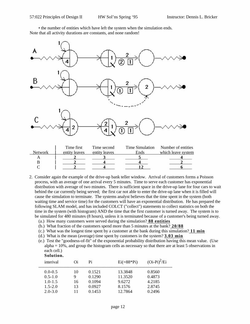
1. For each SLAM network below, state• the time at which the first entity leaves the system• the time at which the simulation ends (or the last entity leaves the system, whichever is first)

page 11


• the number of entities which have left the system when the simulation ends.Note that all activity durations are constants, and none random!

Time first Time second Time Simulation Number of entities Network entity leaves entity leaves Ends which leave system

A _____2____ _____3____ ______5___ _____4____B _____2____ _____4____ ______4___ _____2____C _____2____ _____4____ ______12___ _____6____

2. Consider again the example of the drive-up bank teller window. Arrival of customers forms a Poissonprocess, with an average of one arrival every 5 minutes. Time to serve each customer has exponentialdistribution with average of two minutes. There is sufficient space in the drive-up lane for four cars to waitbehind the car currently being served; the first car not able to enter the drive-up lane when it is filled willcause the simulation to terminate. The systems analyst believes that the time spent in the system (bothwaiting time and service time) for the customers will have an exponential distribution. He has prepared thefollowing SLAM model, and has included COLCT ("collect") statements to collect statistics on both thetime in the system (with histogram) AND the time that the first customer is turned away. The system is tobe simulated for 480 minutes (8 hours), unless it is terminated because of a customer's being turned away.

(a.) How many customers were served during the simulation? 88 entities(b.) What fraction of the customers spend more than 5 minutes at the bank? 20/88(c.) What was the longest time spent by a customer at the bank during this simulation? 11 min(d.) What is the mean (average) time spent by customers in the system? 3.03 min(e.) Test the "goodness-of-fit" of the exponential probability distribution having this mean value. (Use

alpha = 10%, and group the histogram cells as necessary so that there are at least 5 observations ineach cell.)Solution.

interival Oi Pi Ei(=88*Pi) (Oi-Pi)2/Ei-------------------------------------------------------------------------------------------

0.0-0.5 10 0.1521 13.3848 0.85600.5-1.0 9 0.1290 11.3520 0.48731.0-1.5 16 0.1094 9.6272 4.21851.5-2.0 13 0.0927 8.1576 2.87452.0-3.0 11 0.1453 12.7864 0.2496

page 12


3.0-3.5 5 0.0565 4.9720 0.00023.5-5.5 6 0.1522 13.3936 4.08155.5-7.5 8 0.0787 6.9256 0.16677.5-9.0 5 0.0328 2.8864 1.54779.0- 5 0.0513 4,5144 0.0586

-------------------------------------------------------------------------------------------D=14.54

where P1 =1 − e−(0.53.03), P2 = e

− (0.5 3.03) − e−(1.0 3.03) , etc.

Degree of freedom = 10-1-1=8, χ10%,82 = 13.501. Since D>χ10%,8

2 , we reject the hyperthesis.

(f.) At what time does the simulation end? Is it because of the maximum time (480 minutes) or becauseof a customer being turned away? 408 min

1 GEN,BRICKER,BANKTELLER,2/23/1995,,,,,,,72; 2 LIM,2,1,50; 3 INIT,0,480; 4 NETWORK; 5 CREATE,EXPON(5.0),,1; 6 QUE(1),0,4,BALK(OVFLO); 7 ACT(1)/1,EXPON(2.0); 8 COLCT,INTVL(1),CUSTOMER_TIME,20/.5/.5; 9 TERM; 10 OVFLO COLCT,FIRST; 11 TERM,1; 12 END; 13 FIN;

S L A M I I S U M M A R Y R E P O R T SIMULATION PROJECT BANKTELLER BY BRICKER

CURRENT TIME 0.4081E+03 STATISTICAL ARRAYS CLEARED AT TIME 0.0000E+00

**STATISTICS FOR VARIABLES BASED ON OBSERVATION**

MEAN STANDARD COEFF. OF MINIMUM MAXIMUM NO.OF VALUE DEVIATION VARIATION VALUE VALUE OBS

CUSTOMER_TIME 0.303E+01 0.286E+01 0.944E+00 0.345E-01 0.110E+02 88 0.408E+03 0.000E+00 0.000E+00 0.408E+03 0.408E+03 1

page 13


**FILE STATISTICS**

FILE AVERAGE STANDARD MAXIMUM CURRENT AVERAGE NUMBER LABEL/TYPE LENGTH DEVIATION LENGTH LENGTH WAIT TIME

1 QUEUE 0.300 0.724 4 4 1.317 2 0.000 0.000 0 0 0.000 3 CALENDAR 1.439 0.496 3 2 2.669

**SERVICE ACTIVITY STATISTICS**

ACT ACT LABEL OR SER AVERAGE STD CUR AVERAGE MAX IDL MAX BSY ENT NUM START NODE CAP UTIL DEV UTIL BLOCK TME/SER TME/SER CNT

1 QUEUE 1 0.439 0.50 1 0.00 17.35 29.23 88 **HISTOGRAM NUMBER 1** CUSTOMER_TIME

OBS RELA UPPER FREQ FREQ CELL LIM 0 20 40 60 80 100 + + + + + + + + + + + 10 0.114 0.500E+00 +****** + 9 0.102 0.100E+01 +***** C + 16 0.182 0.150E+01 +********* C + 13 0.148 0.200E+01 +******* C + 4 0.045 0.250E+01 +** C + 7 0.080 0.300E+01 +**** C + 5 0.057 0.350E+01 +*** C + 1 0.011 0.400E+01 +* C + 3 0.034 0.450E+01 +** C + 0 0.000 0.500E+01 + C + 2 0.023 0.550E+01 +* C + 1 0.011 0.600E+01 +* C + 3 0.034 0.650E+01 +** C + 0 0.000 0.700E+01 + C + 4 0.045 0.750E+01 +** C + 1 0.011 0.800E+01 +* C + 2 0.023 0.850E+01 +* C + 2 0.023 0.900E+01 +* C + 2 0.023 0.950E+01 +* C + 2 0.023 0.100E+02 +* C+ 0 0.000 0.105E+02 + C+ 1 0.011 INF +* C --- + + + + + + + + + + + 88 0 20 40 60 80 100



CUSTOMER_TIME 0.303E+01 0.286E+01 0.944E+00 0.345E-01 0.110E+02 88Fortran STOP

«»«»«»«»«»«»«»«»«»«»«»«»«»«»«»«» HW #6 «»«»«»«»«»«»«»«»«»«»«»«»«»«»«»«»

Project Scheduling. An equipment maintenance building is to be erected near a large construction site.An electric generator and a large water storage tank are to be installed a short distance away and connected tothe building. The activity descriptions and estimated durations for the project are:

page 14


Duration Activity Description Predecessor(s) optimistic most likely pessimistic

A Clear & level site none 1 2 4B Erect building A 4 6 9C Install generator A 1 3 4D Install water tank A 1 2 4E Install maintenance equipment B 2 4 6F Connect generator & tank to bldg B,C,D 2 5 7G Paint & finish work on building B 2 3 4H Facility test & checkout E,F 1 2 3

a. Draw the AON (activity-on-node) network representing this project.Solution.

AStart

B

C

D

G

E

F

HEnd

b. Draw the AOA (activity-on-arrow) network representing this project. Explain the necessity for any"dummy" activities which you have included.

Solution.

0 1

2

4

3

5 6

AB

C

D

G

E

FH

c. Label the nodes of the AOA network, so that i<j if there is an activity with node i as its start and node jas its end node.

Solution. See above network.

In questions (d) through ( h), use the "most likely" as the duration:

d. Perform the forward pass through the AOA network to obtain for each node i, ET(i) = earliest possibletime for event i.

Solution.

page 15


0 1

2

4

3

5 6

AB

C

D

G

E

FH

0 0

8 8

2 2

4 8

13 13

15 15

8 8

The ET is the first value in the box of above network.

e. What is the earliest completion time for this project?Solution. 15 days.

f. Perform the backward pass through the AOA network to obtain, for each node i, LT(i) = latest possibletime for event i (assuming the project is to be completed in the time which you have specified in (e).)

g. For each activity, compute:ES = earliest start time EF = earliest finish timeLS = latest start time LF = latest finish timeTF = total float (slack)

Solution. Activity ES EF LS LF TFA 0 2 0 2 0B 2 8 6 8 0C 2 5 5 8 3D 2 4 6 8 4E 8 12 9 13 1F 8 13 8 13 0G 8 11 12 15 4H 13 15 13 15 0

h. Which activities are "critical", i.e., have zero float ("slack")?Solution. A, B, F, and H.

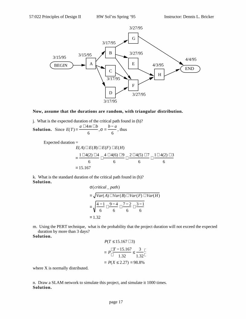
i. Schedule this project by entering the AON network into MacProject II (found on several of the MacintoshII computers in the computer lab on 3rd floor of the Engineering Building.) Specify that the start timefor the project will be March 15, 1995. What is the earliest completion time for the project? (Note that5-day work weeks are assumed by default.)

Solution.

page 16


A

B

C

D

G

E

F

H

BEGINEND

3/15/95 3/15/95

3/17/95

3/17/95

3/17/95

3/27/95

3/27/95

3/27/95

4/3/954/4/95

Now, assume that the durations are random, with triangular distribution.

j. What is the expected duration of the critical path found in (h)?

Solution. Since E(T ) =a + 4m + b

6,σ =

b − a

6, thus

Expected duration =E( A) + E(B) + E(F) + E(H)

=1 + 4(2) + 4

6+

4 + 4(6) + 9

6+

2 + 4(5) + 7

6+

1+ 4(2) + 3

6= 15.167

k. What is the standard duration of the critical path found in (h)?Solution.

σ(critical _ path)

= Var( A) + Var(B) + Var(F) + Var(H )

= 4 −1

6+ 9 − 4

6+ 7 − 2

6+ 3 −1

6

= 1.32

m. Using the PERT technique, what is the probability that the project duration will not exceed the expectedduration by more than 3 days?

Solution.P(T ≤15.167 + 3)

= PT −15.167

1.32≤

3

1.32

= P(X ≤ 2.27) = 98.8%where X is normally distributed.

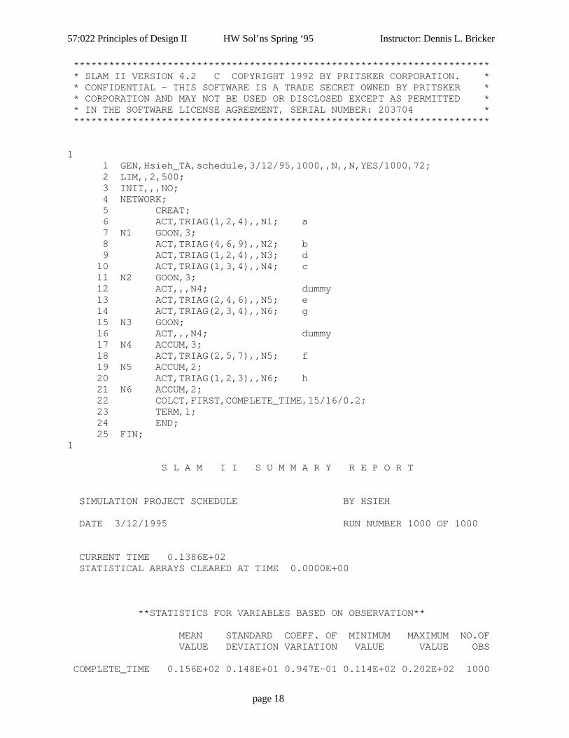
n. Draw a SLAM network to simulate this project, and simulate it 1000 times.Solution.

page 17


*********************************************************************** * SLAM II VERSION 4.2 C COPYRIGHT 1992 BY PRITSKER CORPORATION. * * CONFIDENTIAL - THIS SOFTWARE IS A TRADE SECRET OWNED BY PRITSKER * * CORPORATION AND MAY NOT BE USED OR DISCLOSED EXCEPT AS PERMITTED * * IN THE SOFTWARE LICENSE AGREEMENT, SERIAL NUMBER: 203704 * ***********************************************************************

1 1 GEN,Hsieh_TA,schedule,3/12/95,1000,,N,,N,YES/1000,72; 2 LIM,,2,500; 3 INIT,,,NO; 4 NETWORK; 5 CREAT; 6 ACT,TRIAG(1,2,4),,N1; a 7 N1 GOON,3; 8 ACT,TRIAG(4,6,9),,N2; b 9 ACT,TRIAG(1,2,4),,N3; d 10 ACT,TRIAG(1,3,4),,N4; c 11 N2 GOON,3; 12 ACT,,,N4; dummy 13 ACT,TRIAG(2,4,6),,N5; e 14 ACT,TRIAG(2,3,4),,N6; g 15 N3 GOON; 16 ACT,,,N4; dummy 17 N4 ACCUM,3; 18 ACT,TRIAG(2,5,7),,N5; f 19 N5 ACCUM,2; 20 ACT,TRIAG(1,2,3),,N6; h 21 N6 ACCUM,2; 22 COLCT,FIRST,COMPLETE_TIME,15/16/0.2; 23 TERM,1; 24 END; 25 FIN;1

S L A M I I S U M M A R Y R E P O R T

SIMULATION PROJECT SCHEDULE BY HSIEH

DATE 3/12/1995 RUN NUMBER 1000 OF 1000




COMPLETE_TIME 0.156E+02 0.148E+01 0.947E-01 0.114E+02 0.202E+02 1000

page 18


1 **HISTOGRAM NUMBER 1** COMPLETE_TIME

OBS RELA UPPER FREQ FREQ CELL LIM 0 20 40 60 80 100 + + + + + + + + + + + 605 0.605 0.160E+02 +****************************** + 57 0.057 0.162E+02 +*** C + 49 0.049 0.164E+02 +** C + 38 0.038 0.166E+02 +** C + 37 0.037 0.168E+02 +** C + 31 0.031 0.170E+02 +** C + 33 0.033 0.172E+02 +** C + 33 0.033 0.174E+02 +** C + 34 0.034 0.176E+02 +** C + 14 0.014 0.178E+02 +* C + 13 0.013 0.180E+02 +* C + 13 0.013 0.182E+02 +* C + 13 0.013 0.184E+02 +* C+ 5 0.005 0.186E+02 + C+ 5 0.005 0.188E+02 + C+ 5 0.005 0.190E+02 + C+ 15 0.015 INF +* C --- + + + + + + + + + + + *** 0 20 40 60 80 100



COMPLETE_TIME 0.156E+02 0.148E+01 0.947E-01 0.114E+02 0.202E+02 1000Fortran STOP

o. What is the average duration of the project according to SLAM? (Compare it to your answer in (j).)Solution. 15.6 which is larger than 15.167 in (j).

p. What is the standard deviation of the project duration according to SLAM? (Compare it to your answerin (k).)

Solution. 1.48 which is larger than 1.32 in (j).

q. According to the SLAM simulation, what is the probability that the project duration will not exceed theexpected duration by more than three days?

Solution. By the CDF figure, we haveP(T ≤15.6 + 3)

= 1 − P(T > 18.6)

= 1 − 5 + 5 +15

1000= 99.75%

.

«»«»«»«»«»«»«»«»«»«»«»«»«»«»«»«» HW #7 «»«»«»«»«»«»«»«»«»«»«»«»«»«»«»«»

page 19


1. Markov Chain Model of a Reservoir: A city's water supply comes from a reservoir. Careful studyof this reservoir over the past twenty years has shown that, if the reservoir was full at the beginning of onesummer, then the probability that it would be full at the beginning of the next summer is 80%; however, if thereservoir was not full at the beginning of one summer, the probability that it would be full at the beginning ofthe next summer is only 40%.

The below computer output may be consulted to help answer some of the following questions. Note that state#1 represents the condition "full" and state #2 represents the condition "not full"

a. Draw a diagram of a Markov Chain model of this reservoir.Solution.

0.800.20

0.40

0.60

1 2

page 20


b. Why are we guaranteed that this system has a steady-state probability distribution?Solution. Since this Markov chain is regular.

c. Write equations which could be solved to compute the steady-state distribution. (You need not solvethem!)

Solution.

(π1, π2 ) = (π1,π 2 )0.8 0.2

0.4 0.6

, or

π1 = 0.8π1 + 0.4 π2

π2 = 0.2π1 + 0.6π2

d. Over a 100-year period, how many summers can the reservoir be expected to be full?

Solution.100π1 =100(0.6667) = 67

e. If the reservoir was full at the beginning of summer 1994, what is the probability that• it will be full at the beginning of summer 1995?

Solution. P11

1 =0.8.

• it will be full at the beginning of summer 1996?

Solution. P11

2 =0.72.

f. If the reservoir was full at the beginning of summer 1994, what is the expected number of summersduring the next 5 years that the reservoir will not be full?

Solution. 1.44672 (by the matrix of Expected no. of visits during first 5 years)

g. If the reservoir was full at the beginning of summer 1994, what is the expected number of yearsbefore the reservoir will not be full at the beginning of the summer?

Solution. 5 (by the matrix of Mean First Passage Times)

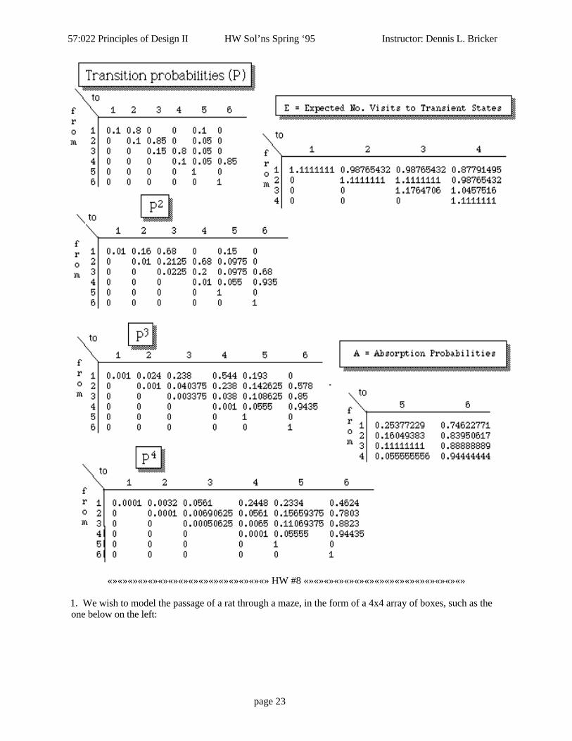
2. Absorption Analysis of Markov Chain. In response to pressure from the Board of Regents toincrease the number of students who complete their degrees within four years, the Engineering Collegeadmissions office has modeled the academic career of a student as a Markov chain:

Each student's state is observed at the beginning of each fall semester. For example, if a student is a junior atthe beginning of the current fall semester, there is an 80% chance that he/she will be a senior at the beginningof the next fall semester, a 15% chance that he/she will still be a junior, and a 5% chance that he/she will havequit. (For simplicity we will assume that once a student quits, he/she never re-enrolls.)

State Description1 Freshman2 Sophomore3 Junior4 Senior5 Drop-out6 Graduate

a. Draw a diagram for this Markov chain.Solution. By the P matrix, we may draw the diagram as

page 21


1 2 3 4

0.1

0.8

0.1

0.1 0.15 0.1 1.0

1.0

0.050.050.05

0.85 0.8 0.856

5

b. Which states are transient?Solution. 1,2,3, and 4.

c. Which states are recurrent?Solution. 5 and 6.

d. Which states are absorbing?Solution. 5 and 6.

e. Does this system have a steady-state probability distribution? Justify your answer.Solution. No. Since there are some absorbing states, the steady-state probabilities will be

based on the initial probabilities.

Consult the computer output below to answer the questions that follow.

f. If a student enters the college as a freshman, how many years can he or she expect to spend as astudent in the college?

Solution. By E matrix, we have 1.1111+ 0.9877 + 0.9877 + 0.8779 = 3.9643 (years).

g. What is the probability that, at the beginning of the fourth year in the college, he or she is classifiedas a senior?

Solution. P14

3 = 0.544 .

h. What is the probability that he or she eventually will graduate?Solution. Assume that he is a freshman now. By A matrix we have the probability is

A16 = 0.7462 .

i. If a student has survived to the point that he or she has been classified as a junior, what is then theprobability that he or she eventually graduates?

Solution. By matrix A we have A36 = 0.8889 .

page 22


«»«»«»«»«»«»«»«»«»«»«»«»«»«»«»«» HW #8 «»«»«»«»«»«»«»«»«»«»«»«»«»«»«»«»

1. We wish to model the passage of a rat through a maze, in the form of a 4x4 array of boxes, such as theone below on the left:

page 23


The solid lines represent walls, the shaded lines represent doors. We will assume that a rat is placedinto box #1. While in any box, the rat is assumed to be equally likely to choose each of the doorsleaving the box (including the one by which he entered the box). For example, when in box #2above, the probability of going next to boxes 3 and 6 are each 1/2, regardless of the door by whichhe entered the box. This assumption implies that no learning takes place if the rat tries the mazeseveral times. (Note that the assumptions imply that the mouse is as equally likely to exit a box bythe door through which he entered as any of the other exiting doors.)

Based upon this "memorylessness" assumption, the movement of the rat through the maze can be modeled asa discrete-time Markov chain:

page 24


The steadystate probability distribution exists because the chain is regular, and is:

The mean first passage time matrix (M) is

The first-visit probabilities from box #1 to the reward in box #16 are:

The shortest path from box 1 to box 16 is: 1->5->6->7->11->15->16, or 6 moves. The matrix P6 is

page 25


a. Which box will be visited most frequently by the rat?Solution. Box #11.

b. A reward (e.g. food) is placed in box #16 for the rat. What is the expected number of moves of therat required to reach this reward?

Solution. 87.3

c. The minimum number of moves required to reach the reward is six. What is the probability that therat reaches the reward in exactly this number of moves?

Solution. 0.006494

d. What is the probability that the rat reaches the reward with no more than 4 unnecessary moves?Solution. 0.006494+0.0126+0.0165=0.03604

e. Briefly discuss the utility of this model in testing a hypothesis that a real rat is able to learn, therebyfinding the reward in relatively few moves after he has made several trial runs through the maze.

Solution. (omitted)

page 26


f. Briefly discuss how you might modify your Markov chain model if the rat will never exit a box bythe same door through which he entered (i.e., he is no longer completely "memoryless", in that heremembers the door through which he entered), unless he has reached a "dead end", in which casehe reverses his path.

Solution. (omitted)

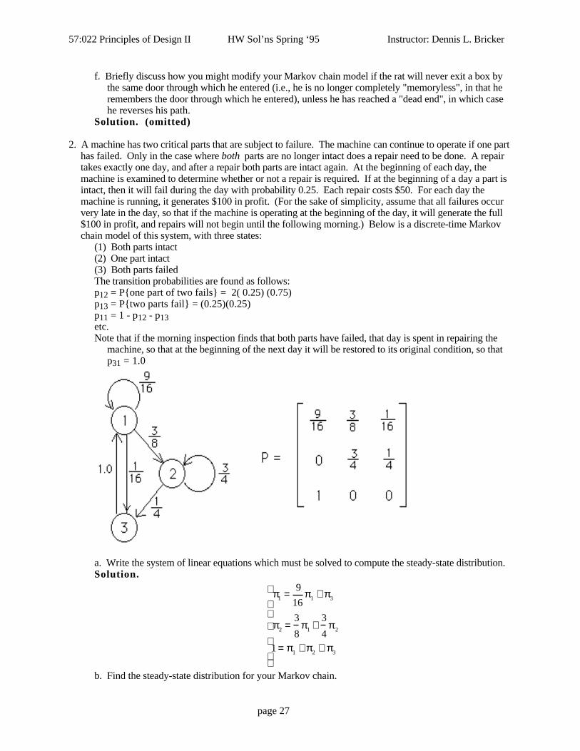
2. A machine has two critical parts that are subject to failure. The machine can continue to operate if one parthas failed. Only in the case where both parts are no longer intact does a repair need to be done. A repairtakes exactly one day, and after a repair both parts are intact again. At the beginning of each day, themachine is examined to determine whether or not a repair is required. If at the beginning of a day a part isintact, then it will fail during the day with probability 0.25. Each repair costs $50. For each day themachine is running, it generates $100 in profit. (For the sake of simplicity, assume that all failures occurvery late in the day, so that if the machine is operating at the beginning of the day, it will generate the full$100 in profit, and repairs will not begin until the following morning.) Below is a discrete-time Markovchain model of this system, with three states:

(1) Both parts intact(2) One part intact(3) Both parts failedThe transition probabilities are found as follows:p12 = P{one part of two fails} = 2( 0.25) (0.75)p13 = P{two parts fail} = (0.25)(0.25)p11 = 1 - p12 - p13etc.Note that if the morning inspection finds that both parts have failed, that day is spent in repairing the

machine, so that at the beginning of the next day it will be restored to its original condition, so thatp31 = 1.0

a. Write the system of linear equations which must be solved to compute the steady-state distribution.Solution.

π1 = 9

16π1 + π3

π2 =3

8π1 +

3

4π 2

1 = π1 + π2 + π3

b. Find the steady-state distribution for your Markov chain.

page 27


Solution.

π1 =16

47,π2 =

24

47, π3 =

7

47

c. Compute the average profit per day for this machine.Solution. 100(π1 + π2 ) − 50π3 = 77.6

3. (Exercise 6, page 1083-1084 of text by Winston) Bectol, Inc. is building a dam. A total of 10,000,000cu ft of dirt is needed to construct the dam. A bulldozer is used to collect dirt for the dam. Then the dirt ismoved via dumpers to the dam site. Only one bulldozer is available, and it rents for $100 per hour. Bectolcan rent, at $40 per hour, as many dumpers as desired. Each dumper can hold 1000 cu ft of dirt. It takes anaverage of 12 minutes for the bulldozer to load a dumper with dirt, and it takes each dumper an average of fiveminutes to deliver the dirt to the dam and return to the bulldozer. Making appropriate assumptions aboutexponentiality so as to obtain a birth/death model, determine the optimal number of dumpers and the minimumtotal expected cost of moving the dirt needed to build the dam.

Hint: We have to use 10,000,000/1000=10,000 loads of dumper to deliver all the dirt.

Case 1 : One dumper :Define state 0 : no dumper in the system,

state 1 : one dumper in the system.Then we obtain a birth/death model:

0 1

12/hr

5/hr

Steady-state Distribution------------------------------i Pi CDF- ------------ -----------0 0.294118 0.2941181 0.705882 1.000000

where the steady-state distribution is found by1π0

= 1 + 12 hr5 hr

= 175

⇒ π0= 517

, etc.

The average departure rate of dumper is (1-π0)5=0.705882(5)=3.52941(times/hr)The total cost = (10,000/3.52941)($100+$40)=396667.

Use trial & error to find the optimal number of dumpers.Solution.(1) One dumper: Total cost = 396667(2) Two dumpers:

24/hr 12/hr

5/hr 5/hr

0 1 2

1

π 0

= 1 +24

5+

24

5

12

5

= 17.32

(1− π0 )5 = 4.711316

10000

4.711316100 + 40 + 40( ) = 382059

Total cost = 382059(3) Three dumpers:

page 28


24/hr 12/hr

5/hr 5/hr

0 1 2 3

36/hr

5/hr

1

π 0

= 1 +36

5+

36

5

24

5+

36

5

24

5

12

5

= 125.704

(1− π0 )5 = 4.960224

10000

4.960224100 + 40 + 40 + 40( ) = 443528

Total cost = 443528

Thus the optimal solution is 2 dumpers.

«»«»«»«»«»«»«»«»«»«»«»«»«»«»«»«» HW #9 «»«»«»«»«»«»«»«»«»«»«»«»«»«»«»«»

The following exercises are done assuming that the queueing systems operatesin steady state.

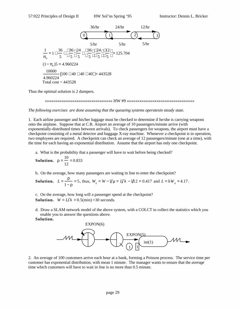
1. Each airline passenger and his/her luggage must be checked to determine if he/she is carrying weaponsonto the airplane. Suppose that at C.R. Airport an average of 10 passengers/minute arrive (withexponentially-distributed times between arrivals). To check passengers for weapons, the airport must have acheckpoint consisting of a metal detector and baggage X-ray machine. Whenever a checkpoint is in operation,two employees are required. A checkpoint can check an average of 12 passengers/minute (one at a time), withthe time for each having an exponential distribution. Assume that the airport has only one checkpoint.

a. What is the probability that a passenger will have to wait before being checked?

Solution. ρ =10

12= 0.833

b. On the average, how many passengers are waiting in line to enter the checkpoint?

Solution. L =ρ

1 − ρ= 5, thus, Wq = W −1 µ = L λ −112 = 0.417 and L = λWq = 4.17.

c. On the average, how long will a passenger spend at the checkpoint?Solution. W = L λ = 0.5(min) =30 seconds.

d. Draw a SLAM network model of the above system, with a COLCT to collect the statistics which youenable you to answer the questions above.

Solution.

int(1)

EXPON(6)

EXPON(5)

1 1

2. An average of 100 customers arrive each hour at a bank, forming a Poisson process. The service time percustomer has exponential distribution, with mean 1 minute. The manager wants to ensure that the averagetime which customers will have to wait in line is no more than 0.5 minute.

page 29


a. If the bank follows the policy of having all customers join a single queue to wait for a teller, howmany tellers should the bank hire?

Solution. Wq = Lq λ =3

5Lq <

1

2From the formula for M/M/C in classnotes, we have

If C=2, then π 0 =1

11, Lq =

50

11

If C=3, then π 0 =24

139, Lq =

125(3)

(139)4<

1

2.

Hence 3 tellers are needed.

b. Draw a SLAM network model of the above system, with a COLCT to collect the statistics which youenable you to answer the question above.

Solution.

int(1)

EXPON(1)

3 1

EXPON(0.6)

3. An average of 60 cars per hour arrive (forming a Poisson process) arrive at the MacBurger's drive-inwindow. However, if four or more cars are in line (including the car at the window), an arriving car will notenter the line (i.e., "balk"). It takes an average of 3 minutes (exponentially distributed) to serve a car.

a. What is the average number of cars waiting for the drive-in window (not including a car at thewindow)?

Solution. This is a M/M/N Queue, where N=4.Thus, from the formula in classnotes, we get

π 0 = 0.0083, π1 = 0.0248, π2 = 0.0743, π3 = 0.2230, π4 = 0.6690

Lq = (n −1)πn

n= 2

4

∑ ≈ 2.3

b. On the average, how many cars will be served per hour?Solution. 60/3=20 (cars)

c. If you have just joined the line, how many minutes will you expect to pass before you receive yourfood?

Solution. W =L

λ (1− π N )= 10.6 (min)

d. Draw a SLAM network model of the above system, with a COLCT to collect the statistics which youenable you to answer the questions above.

Solution.

page 30


int(1)

EXPON(3)

3 1

EXPON(1)

4

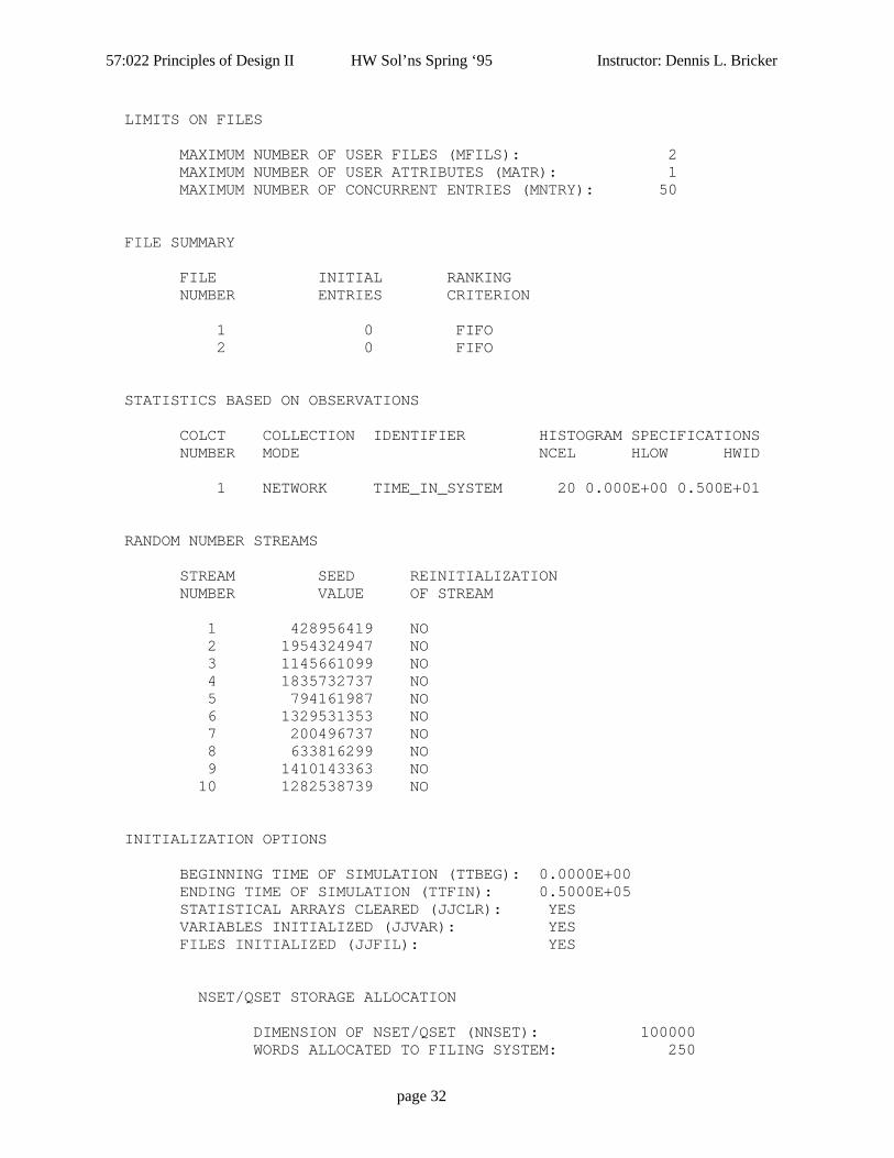
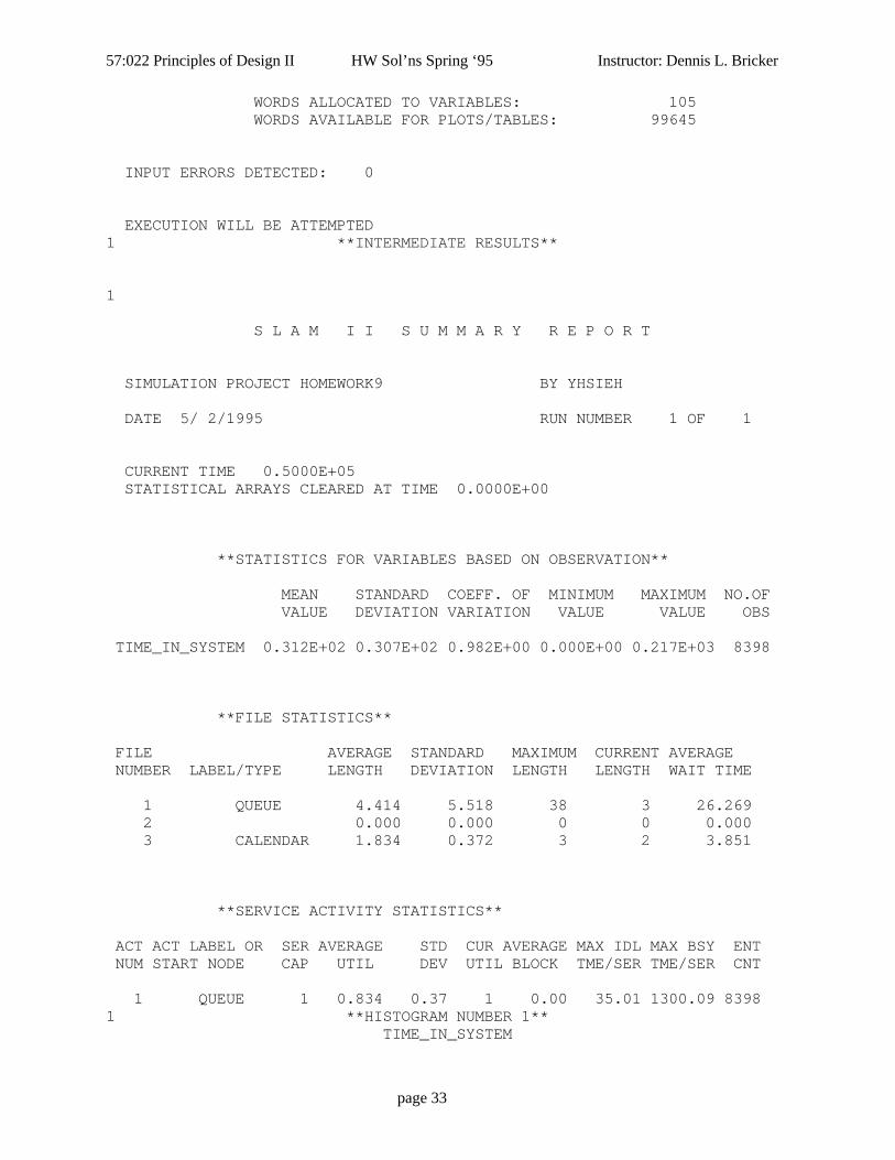
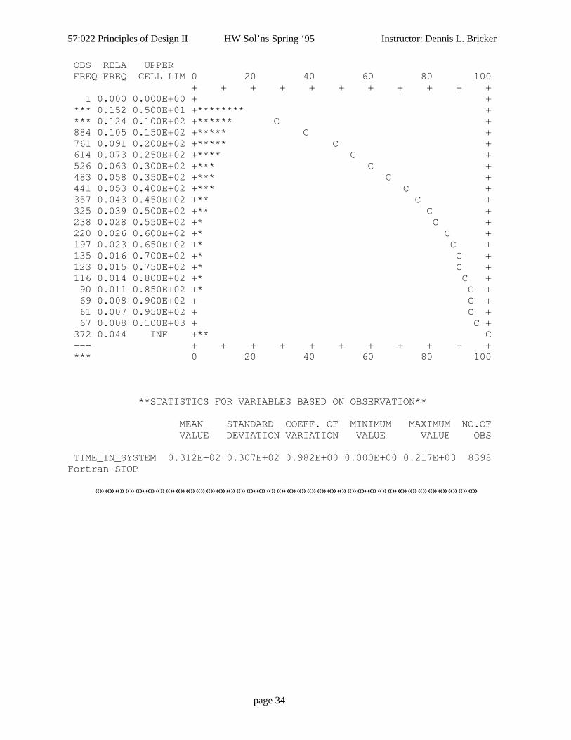
4. Choose one of the three SLAM networks above, and simulate it on the computer for an 8-hour period.Compare the simulation results with your previous answers based upon steadystate queueing theory.Solution. The following is the slam code for Problem (1), we find that(a) the probability that a passenger will have to wait is 0.833 in problem (1) and 0.834 in simulation(b) the number of passengers in line is 4.17 for problem(1), and 4.414 by simulation(c) waiting time in the system is 30 seconds, and 31.2 seconds by simulationThat is the simulation values are very close to the theoretical values.

1 1 GEN,yhsieh,Homework9,5/2/95,,,,,,,72; 2 LIM,2,1,50; 3 INIT,0,50000; 4 NETWORK; 5 CREATE,EXPON(6),,1; 6 QUE(1); 7 ACT(1)/1,EXPON(5); 8 COLCT,INTVL(1),Time_in_system,20/0/5; 9 TERM; 10 END; 11 FIN;1

S L A M I I E C H O R E P O R T

SIMULATION PROJECT HOMEWORK9 BY YHSIEH

DATE 5/ 2/1995 RUN NUMBER 1 OF 1

SLAM II VERSION AUG 92

GENERAL OPTIONS

PRINT INPUT STATEMENTS (ILIST): YES PRINT ECHO REPORT (IECHO): YES EXECUTE SIMULATIONS (IXQT): YES WARN OF DESTROYED ENTITIES: YES PRINT INTERMEDIATE RESULTS HEADING (IPIRH): YES PRINT SUMMARY REPORT (ISMRY): YES

page 31


LIMITS ON FILES

MAXIMUM NUMBER OF USER FILES (MFILS): 2 MAXIMUM NUMBER OF USER ATTRIBUTES (MATR): 1 MAXIMUM NUMBER OF CONCURRENT ENTRIES (MNTRY): 50

FILE SUMMARY

FILE INITIAL RANKING NUMBER ENTRIES CRITERION

1 0 FIFO 2 0 FIFO

STATISTICS BASED ON OBSERVATIONS

COLCT COLLECTION IDENTIFIER HISTOGRAM SPECIFICATIONS NUMBER MODE NCEL HLOW HWID

1 NETWORK TIME_IN_SYSTEM 20 0.000E+00 0.500E+01

RANDOM NUMBER STREAMS

STREAM SEED REINITIALIZATION NUMBER VALUE OF STREAM

1 428956419 NO 2 1954324947 NO 3 1145661099 NO 4 1835732737 NO 5 794161987 NO 6 1329531353 NO 7 200496737 NO 8 633816299 NO 9 1410143363 NO 10 1282538739 NO

INITIALIZATION OPTIONS

BEGINNING TIME OF SIMULATION (TTBEG): 0.0000E+00 ENDING TIME OF SIMULATION (TTFIN): 0.5000E+05 STATISTICAL ARRAYS CLEARED (JJCLR): YES VARIABLES INITIALIZED (JJVAR): YES FILES INITIALIZED (JJFIL): YES

NSET/QSET STORAGE ALLOCATION

DIMENSION OF NSET/QSET (NNSET): 100000 WORDS ALLOCATED TO FILING SYSTEM: 250

page 32


WORDS ALLOCATED TO VARIABLES: 105 WORDS AVAILABLE FOR PLOTS/TABLES: 99645

INPUT ERRORS DETECTED: 0

EXECUTION WILL BE ATTEMPTED1 **INTERMEDIATE RESULTS**

1

S L A M I I S U M M A R Y R E P O R T

SIMULATION PROJECT HOMEWORK9 BY YHSIEH

DATE 5/ 2/1995 RUN NUMBER 1 OF 1




TIME_IN_SYSTEM 0.312E+02 0.307E+02 0.982E+00 0.000E+00 0.217E+03 8398

**FILE STATISTICS**

FILE AVERAGE STANDARD MAXIMUM CURRENT AVERAGE NUMBER LABEL/TYPE LENGTH DEVIATION LENGTH LENGTH WAIT TIME

1 QUEUE 4.414 5.518 38 3 26.269 2 0.000 0.000 0 0 0.000 3 CALENDAR 1.834 0.372 3 2 3.851

**SERVICE ACTIVITY STATISTICS**

ACT ACT LABEL OR SER AVERAGE STD CUR AVERAGE MAX IDL MAX BSY ENT NUM START NODE CAP UTIL DEV UTIL BLOCK TME/SER TME/SER CNT

1 QUEUE 1 0.834 0.37 1 0.00 35.01 1300.09 83981 **HISTOGRAM NUMBER 1** TIME_IN_SYSTEM

page 33


OBS RELA UPPER FREQ FREQ CELL LIM 0 20 40 60 80 100 + + + + + + + + + + + 1 0.000 0.000E+00 + + *** 0.152 0.500E+01 +******** + *** 0.124 0.100E+02 +****** C + 884 0.105 0.150E+02 +***** C + 761 0.091 0.200E+02 +***** C + 614 0.073 0.250E+02 +**** C + 526 0.063 0.300E+02 +*** C + 483 0.058 0.350E+02 +*** C + 441 0.053 0.400E+02 +*** C + 357 0.043 0.450E+02 +** C + 325 0.039 0.500E+02 +** C + 238 0.028 0.550E+02 +* C + 220 0.026 0.600E+02 +* C + 197 0.023 0.650E+02 +* C + 135 0.016 0.700E+02 +* C + 123 0.015 0.750E+02 +* C + 116 0.014 0.800E+02 +* C + 90 0.011 0.850E+02 +* C + 69 0.008 0.900E+02 + C + 61 0.007 0.950E+02 + C + 67 0.008 0.100E+03 + C + 372 0.044 INF +** C --- + + + + + + + + + + + *** 0 20 40 60 80 100



TIME_IN_SYSTEM 0.312E+02 0.307E+02 0.982E+00 0.000E+00 0.217E+03 8398Fortran STOP

«»«»«»«»«»«»«»«»«»«»«»«»«»«»«»«»«»«»«»«»«»«»«»«»«»«»«»«»«»«»«»«»«»«»«»«»«»«»

page 34

Homework Solutions, Spring 1995 - University of Iowa

Documents

Transcript of Homework Solutions, Spring 1995 - University of Iowa