Homework Problems Stat 479 - Purdue Universityjbeckley/WD/STAT 479/S17/STAT 479 S14...Using the data...
25
Homework Problems Stat 479 April 15, 2014 Chapter 10 91. * A random sample, X1, X2, …, Xn, is drawn from a distribution with a mean of 2/3 and a variance of 1/18. ˆ = (X1 + X2 + … + Xn)/(n-1) is the estimator of the distribution mean θ. Find MSE( ˆ ). 92. * Claim sizes are uniformly distributed over the interval [0, θ]. A sample of 10 claims, denoted by X1, X2, …,X10 was observed and an estimate of θ was obtained using: ˆ = Y = max(X1, X2, …,X10) Recall that the probability density function for Y is: fY(y) = 10y 9 /θ 10 Calculate the mean square error for ˆ for θ =100. 93. * You are given two independent estimates of an unknown quantity θ: a. Estimator A: E( ˆ A) = 1000 and σ( ˆ A) = 400 b. Estimator B: E( ˆ B) = 1200 and σ( ˆ B) = 200 Estimator C is a weighted average of Estimator A and Estimator B such that: ˆ C = (w) ˆ A + (1-w) ˆ B Determine the value of w that minimizes σ( ˆ C).
Transcript of Homework Problems Stat 479 - Purdue Universityjbeckley/WD/STAT 479/S17/STAT 479 S14...Using the data...

Homework Problems
Stat 479
April 15, 2014
Chapter 10
91. * A random sample, X1, X2, …, Xn, is drawn from a distribution with a mean of
2/3 and a variance of 1/18.
= (X1 + X2 + … + Xn)/(n-1) is the estimator of the distribution mean θ.
Find MSE( ).
92. * Claim sizes are uniformly distributed over the interval [0, θ]. A sample of 10
claims, denoted by X1, X2, …,X10 was observed and an estimate of θ was obtained
using:
= Y = max(X1, X2, …,X10)
Recall that the probability density function for Y is:
fY(y) = 10y9/θ10
Calculate the mean square error for for θ =100.
93. * You are given two independent estimates of an unknown quantity θ:
a. Estimator A: E( A) = 1000 and σ( A) = 400
b. Estimator B: E( B) = 1200 and σ( B) = 200
Estimator C is a weighted average of Estimator A and Estimator B such that:
C = (w) A + (1-w) B
Determine the value of w that minimizes σ( C).
Homework Problems
Stat 479
April 15, 2014
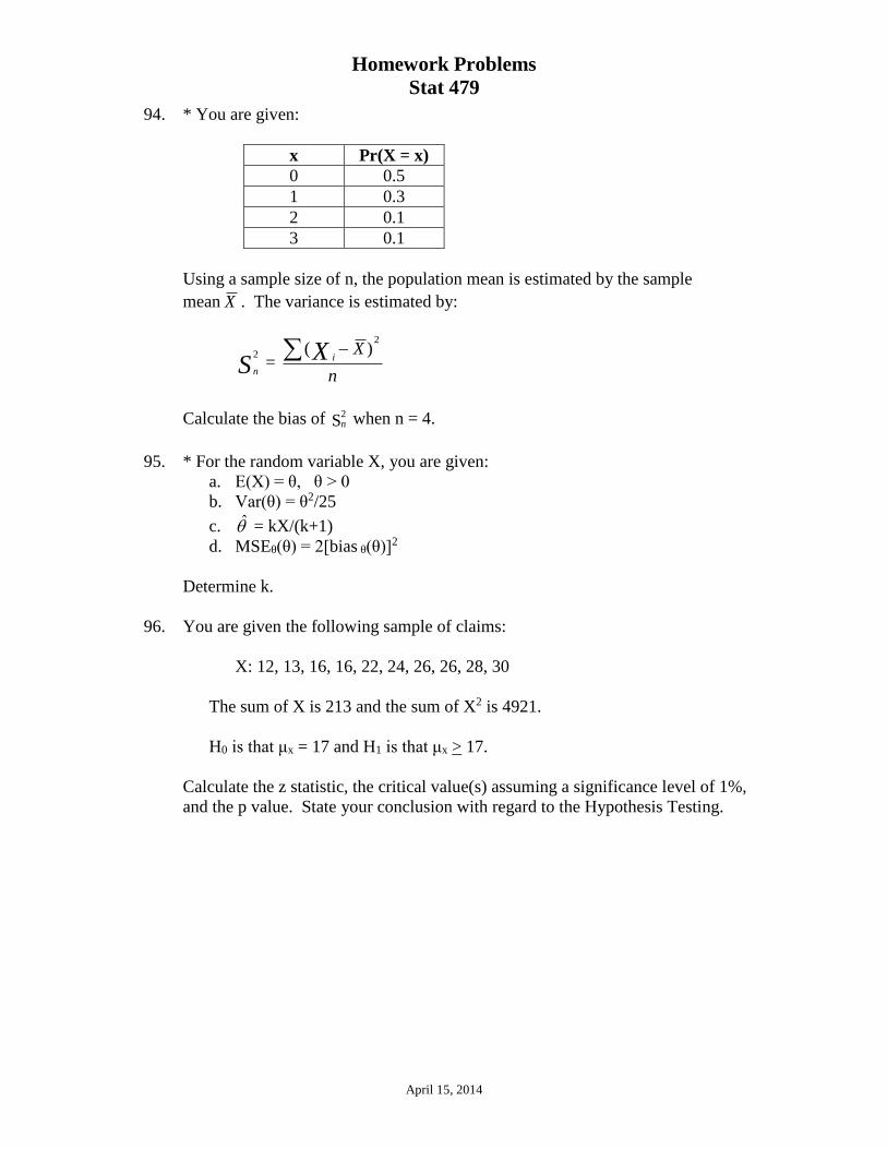
94. * You are given:
x Pr(X = x)
0 0.5
1 0.3
2 0.1
3 0.1
Using a sample size of n, the population mean is estimated by the sample
mean X . The variance is estimated by:
S n
2 =
n
XX i 2
)(
Calculate the bias of S2n when n = 4.
95. * For the random variable X, you are given:
a. E(X) = θ, θ > 0
b. Var(θ) = θ2/25
c. = kX/(k+1)
d. MSEθ(θ) = 2[bias θ(θ)]2
Determine k.
96. You are given the following sample of claims:
X: 12, 13, 16, 16, 22, 24, 26, 26, 28, 30
The sum of X is 213 and the sum of X2 is 4921.
H0 is that μx = 17 and H1 is that μx > 17.
Calculate the z statistic, the critical value(s) assuming a significance level of 1%,
and the p value. State your conclusion with regard to the Hypothesis Testing.
Homework Problems
Stat 479
April 15, 2014
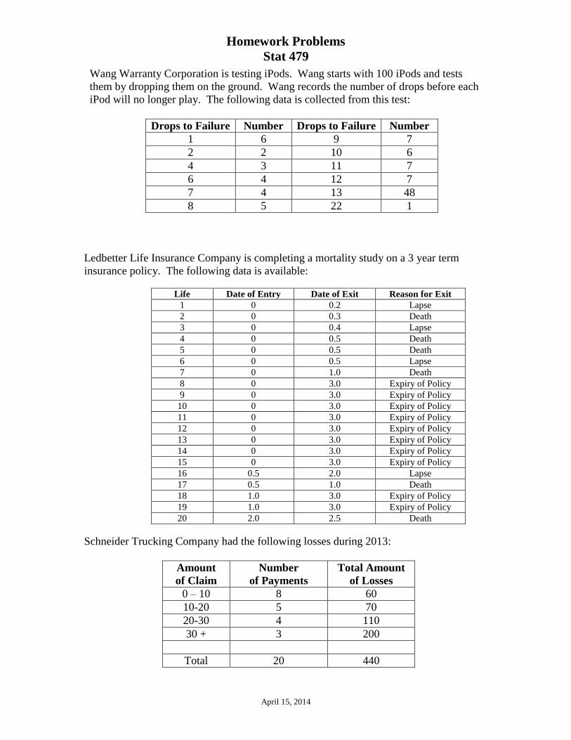
Wang Warranty Corporation is testing iPods. Wang starts with 100 iPods and tests
them by dropping them on the ground. Wang records the number of drops before each
iPod will no longer play. The following data is collected from this test:
Drops to Failure Number Drops to Failure Number
1 6 9 7
2 2 10 6
4 3 11 7
6 4 12 7
7 4 13 48
8 5 22 1
Ledbetter Life Insurance Company is completing a mortality study on a 3 year term
insurance policy. The following data is available:
Life Date of Entry Date of Exit Reason for Exit
1 0 0.2 Lapse
2 0 0.3 Death
3 0 0.4 Lapse
4 0 0.5 Death
5 0 0.5 Death
6 0 0.5 Lapse
7 0 1.0 Death
8 0 3.0 Expiry of Policy
9 0 3.0 Expiry of Policy
10 0 3.0 Expiry of Policy
11 0 3.0 Expiry of Policy
12 0 3.0 Expiry of Policy
13 0 3.0 Expiry of Policy
14 0 3.0 Expiry of Policy
15 0 3.0 Expiry of Policy
16 0.5 2.0 Lapse
17 0.5 1.0 Death
18 1.0 3.0 Expiry of Policy
19 1.0 3.0 Expiry of Policy
20 2.0 2.5 Death
Schneider Trucking Company had the following losses during 2013:
Amount
of Claim
Number
of Payments
Total Amount
of Losses
0 – 10 8 60
10-20 5 70
20-30 4 110
30 + 3 200
Total 20 440
Homework Problems
Stat 479
April 15, 2014
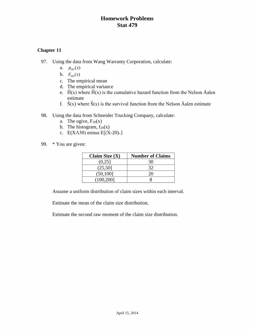
Chapter 11
97. Using the data from Wang Warranty Corporation, calculate:
a. 100 ( )p x
b. 100 ( )F x
c. The empirical mean
d. The empirical variance
e. Ĥ(x) where Ĥ(x) is the cumulative hazard function from the Nelson Åalen
estimate
f. Ŝ(x) where Ŝ(x) is the survival function from the Nelson Åalen estimate
98. Using the data from Schneider Trucking Company, calculate:
a. The ogive, F20(x)
b. The histogram, f20(x)
c. E(XΛ30) minus E[(X-20)+]
99. * You are given:
Claim Size (X) Number of Claims
(0,25] 30
(25,50] 32
(50,100] 20
(100,200] 8
Assume a uniform distribution of claim sizes within each interval.
Estimate the mean of the claim size distribution.
Estimate the second raw moment of the claim size distribution.

Homework Problems
Stat 479
April 15, 2014
Chapter 12
100. Using the data for Ledbetter Life Insurance Company, calculate the following
where death is the decrement of interest:
a. 20 ( )S t using the Kaplan Meier Product Limit Estimator
b. Ĥ(t) where Ĥ(t) is the cumulative hazard function from the Nelson Åalen
estimate
c. Ŝ(t) where Ŝ(t) is the survival function from the Nelson Åalen estimate
101. Using the data for Ledbetter Life Insurance Company, and treating all expiries as
lapses, calculate the following where lapse is the decrement of interest:
a. 20 ( )S t using the Kaplan Meier Product Limit Estimator
b. Ĥ(t) where Ĥ(t) is the cumulative hazard function from the Nelson Åalen
estimate
c. Ŝ(t) where Ŝ(t) is the survival function from the Nelson Åalen estimate
102. * Three hundred mice were observed at birth. An additional 20 mice were first
observed at age 2 (days) and 30 more were first observed at age 4.
There were 6 deaths at age 1, 10 at age 3, 10 at age 4, a at age 5, b at age 9, and
6 at age 12.
In addition, 45 mice escaped and were lost to observation at age 7, 35 at age 10,
and 15 at age 13.
The following product-limit estimates were obtained:
350 350(7) 0.892 and (13) 0.856S S .
Determine a and b .
103. * There are n lives observed from birth. None are censored and no two lives die
at the same age. At the time of the ninth death, the Nelson Åalen estimate of the
cumulative hazard rate is 0.511 and at the time of the tenth death it is 0.588.
Estimate the value of the survival function at the time of the third death.

Homework Problems
Stat 479
April 15, 2014
104. Astleford Ant Farm is studying the life expectancy of ants. The farm is owned by two
brothers who are both actuaries. They isolate 100 ants and record the following data:
Number of Days till Death Number of Ants Dying
1 4
2 8
3 12
4 20
5 40
6 8
7 4
8 2
9 1
10 1
a. One of the brothers, Robert, uses the Nelson-Åalen estimator to determine ˆ (5)H . Determine the 90% linear confidence interval for ˆ (5)H .
b. The other brother, Daniel, decides that since he has complete data for
these 100 ants, he will just use the unbiased estimator of ˆ(5)S . Using this
approach, determine the 90% confidence interval for ˆ(5)S .

Homework Problems
Stat 479
April 15, 2014
105. The following information on students in the actuarial program at Purdue is used to
complete an analysis of students leaving the program because they are switching majors.
Student Time of
Entry
Time of Exit Reason for Exit
1 0 .5 Switching Major
2-5 0 1 Switching Major
6 0 2 Switching Major
7 0 3 Graduation
8 0 3 Switching Major
9-12 0 3.5 Graduation
13-23 0 4 Graduation
24 0.5 2 Switching Major
25 0.5 3 Switching Major
26 1 3.5 Graduation
27 1 4 Switching Major
28 1.5 4 Graduation
29 2 5 Graduation
30 3 5 Graduation
ˆ( )S x is estimated using the product limit estimator.
Estimate 30[ (2)]Var S using the Greenwood approximation.
106. A mortality study is conducted on 50 lives, all from age 0. At age 15, there were
two deaths; at age 17, there were three censored observations; at age 25 there
were four deaths; at age 30, there were c censored observations; at age 32 there
were eight deaths; and at age 40 there were two deaths.
Let S be the product limit estimate of (35)S and let V be the Greenwood
estimate of this estimator’s variance. You are given 2/ 0.011467.V S
Determine c .
Homework Problems
Stat 479
April 15, 2014
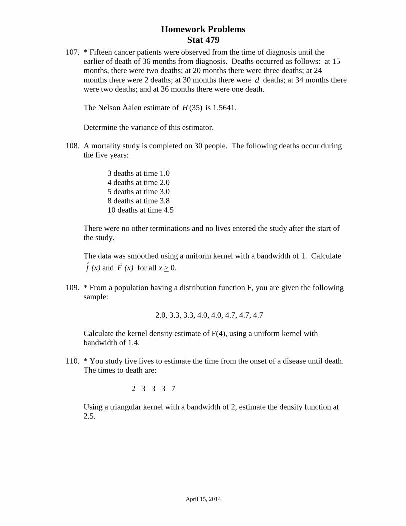
107. * Fifteen cancer patients were observed from the time of diagnosis until the
earlier of death of 36 months from diagnosis. Deaths occurred as follows: at 15
months, there were two deaths; at 20 months there were three deaths; at 24
months there were 2 deaths; at 30 months there were d deaths; at 34 months there
were two deaths; and at 36 months there were one death.
The Nelson Åalen estimate of (35)H is 1.5641.
Determine the variance of this estimator.
108. A mortality study is completed on 30 people. The following deaths occur during
the five years:
3 deaths at time 1.0
4 deaths at time 2.0
5 deaths at time 3.0
8 deaths at time 3.8
10 deaths at time 4.5
There were no other terminations and no lives entered the study after the start of
the study.
The data was smoothed using a uniform kernel with a bandwidth of 1. Calculate
f (x) and F (x) for all x > 0.
109. * From a population having a distribution function F, you are given the following
sample:
2.0, 3.3, 3.3, 4.0, 4.0, 4.7, 4.7, 4.7
Calculate the kernel density estimate of F(4), using a uniform kernel with
bandwidth of 1.4.
110. * You study five lives to estimate the time from the onset of a disease until death.
The times to death are:
2 3 3 3 7
Using a triangular kernel with a bandwidth of 2, estimate the density function at
2.5.

Homework Problems
Stat 479
April 15, 2014
111. You are given the following random sample:
12 15 27 42
The data is smoothed using a uniform kernel with a bandwidth of 6.
Calculate the mean and variance of the smoothed distribution.
112. You are given the following random sample:
12 15 27 42
The data is smoothed using a triangular kernel with a bandwidth of 12.
Calculate the mean and variance of the smoothed distribution.
113. You are given the following random sample:
12 15 27 42
The data is smoothed using a gamma kernel with a bandwidth of 3.
Calculate the mean and variance of the smoothed distribution.

Homework Problems
Stat 479
April 15, 2014
Chapter 13
114. You are given the following sample of claims obtained from an inverse gamma
distribution:
X: 12, 13, 16, 16, 22, 24, 26, 26, 28, 30
The sum of X is 213 and the sum of X2 is 4921.
Calculate α and θ using the method of moments.
115. * You are given the following sample of five claims:
4 5 21 99 421
Find the parameters of a Pareto distribution using the method of moments.
116. * A random sample of death records yields the follow exact ages at death:
30 50 60 60 70 90
The age at death from which the sample is drawn follows a gamma distribution.
The parameters are estimated using the method of moments.
Determine the estimate of α.
117. * You are given the following:
i. The random variable X has the density function
f(x) = αx-α-1 , 1 < x < ∞, α >1
ii. A random sample is taken of the random variable X.
Calculate the estimate of α in terms of the sample mean using the method of
moments.
118. * You are given the following:
i. The random variable X has the density function f(x) = {2(θ – x)}/θ2, 0 < x < θ
ii. A random sample of two observations of X yields values of 0.50 and 0.70.
Determine θ using the method of moments.
Homework Problems
Stat 479
April 15, 2014
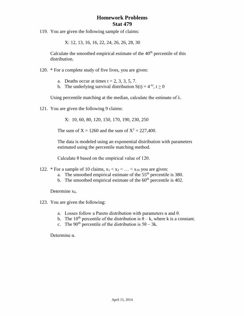
119. You are given the following sample of claims:
X: 12, 13, 16, 16, 22, 24, 26, 26, 28, 30
Calculate the smoothed empirical estimate of the 40th percentile of this
distribution.
120. * For a complete study of five lives, you are given:
a. Deaths occur at times t = 2, 3, 3, 5, 7.
b. The underlying survival distribution S(t) = 4-λt, t > 0
Using percentile matching at the median, calculate the estimate of λ.
121. You are given the following 9 claims:
X: 10, 60, 80, 120, 150, 170, 190, 230, 250
The sum of X = 1260 and the sum of X2 = 227,400.
The data is modeled using an exponential distribution with parameters
estimated using the percentile matching method.
Calculate θ based on the empirical value of 120.
122. * For a sample of 10 claims, x1 < x2 < … < x10 you are given:
a. The smoothed empirical estimate of the 55th percentile is 380.
b. The smoothed empirical estimate of the 60th percentile is 402.
Determine x6.
123. You are given the following:
a. Losses follow a Pareto distribution with parameters α and θ.
b. The 10th percentile of the distribution is θ – k, where k is a constant.
c. The 90th percentile of the distribution is 5θ – 3k.
Determine α.

Homework Problems
Stat 479
April 15, 2014
124. You are given the following random sample of 3 data points from a population
with a Pareto distribution with θ = 70:
X: 15 27 43
Calculate the maximum likelihood estimate for α.
125. * You are given:
a. Losses follow an exponential distribution with mean θ.
b. A random sample of 20 losses is distributed as follows:
Range Frequency
[0,1000] 7
(1000, 2000) 6
(2000,∞) 7
Calculate the maximum likelihood estimate of θ.
126. * You are given the following:
i. The random variable X has the density function f(x) = {2(θ – x)}/θ2, 0 < x < θ
ii. A random sample of two observations of X yields values of 0.50 and 0.90.
Determine the maximum likelihood estimate for θ.
127. * You are given:
a. Ten lives are subject to the survival function S(t) = (1-t/k)0.5, 0 < t < k
b. The first two deaths in the sample occured at time t = 10.
c. The study ends at time t = 10.
Calculate the maximum likelihood estimate of k.
128. * You are given the following:
a. The random variable X follows the exponential distribution with
parameter θ.
b. A random sample of three observations of X yields values of 0.30, 0.55,
and 0.80
Determine the maximum likelihood estimate of θ.
Homework Problems
Stat 479
April 15, 2014
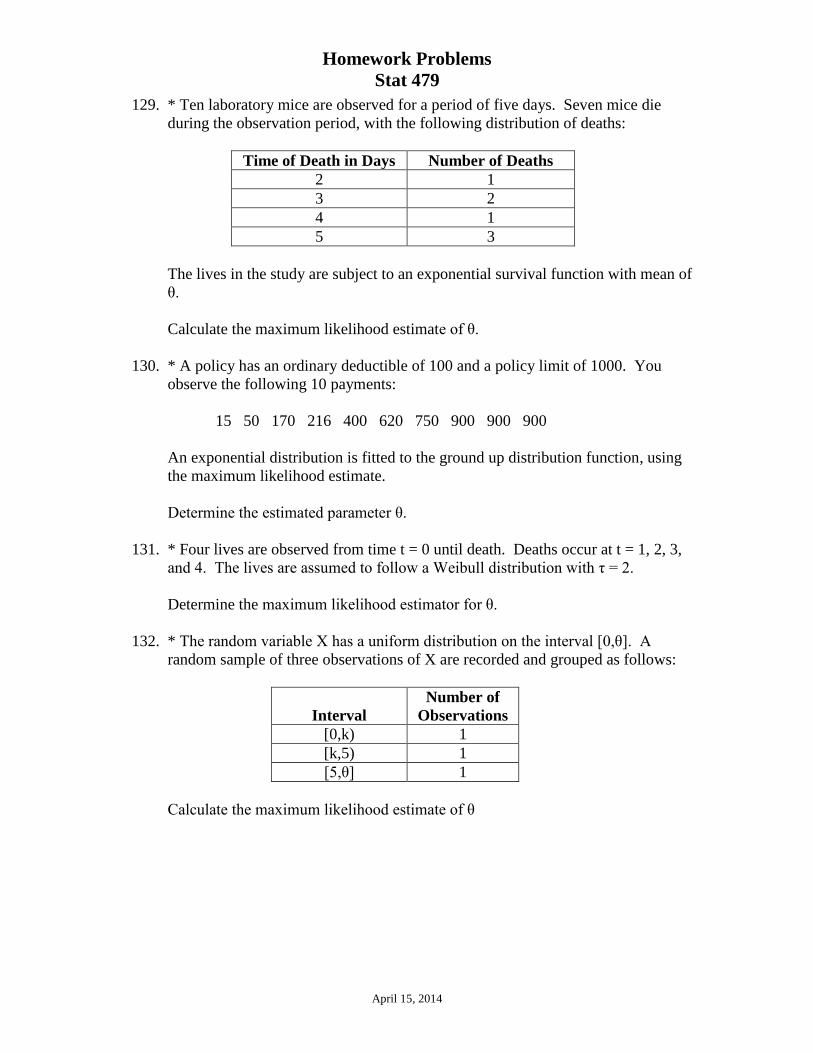
129. * Ten laboratory mice are observed for a period of five days. Seven mice die
during the observation period, with the following distribution of deaths:
Time of Death in Days Number of Deaths
2 1
3 2
4 1
5 3
The lives in the study are subject to an exponential survival function with mean of
θ.
Calculate the maximum likelihood estimate of θ.
130. * A policy has an ordinary deductible of 100 and a policy limit of 1000. You
observe the following 10 payments:
15 50 170 216 400 620 750 900 900 900
An exponential distribution is fitted to the ground up distribution function, using
the maximum likelihood estimate.
Determine the estimated parameter θ.
131. * Four lives are observed from time t = 0 until death. Deaths occur at t = 1, 2, 3,
and 4. The lives are assumed to follow a Weibull distribution with τ = 2.
Determine the maximum likelihood estimator for θ.
132. * The random variable X has a uniform distribution on the interval [0,θ]. A
random sample of three observations of X are recorded and grouped as follows:
Interval
Number of
Observations
[0,k) 1
[k,5) 1
[5,θ] 1
Calculate the maximum likelihood estimate of θ

Homework Problems
Stat 479
April 15, 2014
133. * A random sample of three claims from a dental insurance plan is given below:
225 525 950
Claims are assumed to follow a Pareto distribution with parameters θ = 150 and α.
Determine the maximum likelihood estimate of α.
134. * The following claim sizes are experienced on an insurance coverages:
100 500 1,000 5,000 10,000
You fit a lognormal distribution to this experience using maximum likelihood.
Determine the resulting estimate of σ.
Chapter 14
You are given the following data from a sample:
k nk
0 20
1 25
2 30
3 15
4 8
5 2
Use this data for the next four problems.
135. Assuming a Binomial Distribution, estimate m and q using the Method of
Moments.
136. Assuming a Binomial Distribution, find the MLE of q given that m = 6.
137. (Spreadsheet) Assuming a Binomial Distribution, find the MLE of m and q.
138. Assuming a Poisson Distribution, approximate the 90% confidence interval for
the true value of λ.

Homework Problems
Stat 479
April 15, 2014
Chapter 16
139. You are given the following 20 claims:
X: 10, 40, 60, 65, 75, 80, 120, 150, 170, 190, 230, 340, 430, 440, 980, 600,
675, 950, 1250, 1700
The data is being modeled using an exponential distribution with θ = 427.5.
Calculate D(200).
140. You are given the following 20 claims:
X: 10, 40, 60, 65, 75, 80, 120, 150, 170, 190, 230, 340, 430, 440, 980, 600,
675, 950, 1250, 1700
The data is being modeled using an exponential distribution with θ = 427.5.
You are developing a p-p plot for this data. What are the coordinates for x7 =
120.
141. Mark the following statements True or False with regard to the Kolmogorov-
Smirnov test:
The Kolmogorov-Smirnov test may be used on grouped data as well as
individual data.
If the parameters of the distribution being tested are estimated, the critical
values do not need to be adjusted.
If the upper limit is less than ∞, the critical values need to be larger.

Homework Problems
Stat 479
April 15, 2014
142. Balog’s Bakery has workers’ compensation claims during a month of:
100, 350, 550, 1000
Balog’s owner, a retired actuary, believes that the claims are distributed
exponentially with θ = 500.
He decides to test his hypothesis at a 10% significance level.
Calculate the Kolmogorov-Smirnov test statistic.
State the critical value for his test and state his conclusion.
He also tests his hypothesis using the Anderson-Darling test statistic. State the
values of this test statistic under which Mr. Balog would reject his hypothesis.
143. * The observations of 1.7, 1.6, 1.6, and 1.9 are taken from a random sample. You
wish to test the goodness of fit of a distribution with probability density function
given by f(x) = 0.5x for 0 < x < 2.
Using the Kolmogorov-Smirnov statistic, which of the following should you do?
a. Accept at both levels
b. Accept at the 0.01 level but reject at the 0.10 level
c. Accept at the 0.10 level but reject at the 0.01 level
d. Reject at both levels
e. Cannot be determined.
144. * Two lives are observed beginning at time t=0. One dies at time 5 and the other
dies at time 9. The survival function S(t) = 1 – (t/10) is hypothesized.
Calculate the Kolmogorov-Smirnov statistic.
145. * From a laboratory study of nine lives, you are given:
a. The times of death are 1, 2, 4, 5, 5, 7, 8, 9, 9
b. It has been hypothesized that the underlying distribution is uniform
with ω = 11.
Calculate the Kolmogorov-Smirnov statistic for the hypothesis.

Homework Problems
Stat 479
April 15, 2014
146. You are given the following data:
Claim Range Count
0-100 30
100-200 25
200-500 20
500-1000 15
1000+ 10
H0: The data is from a Pareto distribution.
H1: The data is not from a Pareto distribution.
Your boss has used the data to estimate the parameters as α = 4 and θ = 1200.
Calculate the chi-square test statistic.
Calculate the critical value at a 10% significance level.
State whether you would reject the Pareto at a 10% significance level.
147. During a one-year period, the number of accidents per day in the parking lot of
the Steenman Steel Factory is distributed:
Number of Accidents Days
0 220
1 100
2 30
3 10
4+ 5
H0: The distribution of the number of accidents is distributed as Poison with a
mean of 0.625.
H1: The distribution of the number of accidents is not distributed as Poison with a
mean of 0.625.
Calculate the chi-square statistic.
Calculate the critical value at a 10% significance level.
State whether you would reject the H0 at a 10% significance level.

Homework Problems
Stat 479
April 15, 2014
148. * You are given the following random sample of automobile claims:
54 140 230 560 600 1,100 1,500 1,800 1,920 2,000
2,450 2,500 2,580 2,910 3,800 3,800 3,810 3,870 4,000 4,800
7,200 7,390 11,750 12,000 15,000 25,000 30,000 32,200 35,000 55,000
You test the hypothesis that automobile claims follow a continuous distribution
F(x) with the following percentiles:
x 310 500 2,498 4,876 7,498 12,930
F(x) 0.16 0.27 0.55 0.81 0.90 0.95
You group the data using the largest number of groups such that the expected
number of claims in each group is at least 5.
Calculate the Chi-Square goodness-of-fit statistic.
149. Based on a random sample, you are testing the following hypothesis:
H0: The data is from a population distributed binomial with m = 6 and q = 0.3.
H1: The data is from a population distributed binomial.
You are also given:
L(θ0) = .1 and L(θ1) = .3
Calculate the test statistic for the Likelihood Ratio Test
State the critical value at the 10% significance level
150. State whether the following are true or false
i. The principle of parsimony states that a more complex model is better
because it will always match the data better.
ii. In judgment-based approaches to determining a model, a modeler’s
experience is critical.
iii. In most cases, judgment is required in using a score-based approach to
selecting a model.

Homework Problems
Stat 479
April 15, 2014
Chapter 21
151. A random number generated from a uniform distribution on (0, 1) is 0.6. Using
the inverse transformation method, calculate the simulated value of X assuming:
i. X is distributed Pareto with α = 3 and θ = 2000
0.5x 0 < x < 1.2
ii. F(x) = 0.6 1.2 < x < 2.4
0.5x -0.6 2.4 < x < 3.2
iii. F(x) = 0.1x -1 10 < x < 15
0.05x 15 < x < 20
152. * You are given that f(x) = (1/9)x2 for 0 < x < 3.
You are to simulate three observations from the distribution using the inversion
method. The follow three random numbers were generated from the uniform
distribution on [0,1]:
0.008 0.729 0.125
Using the three simulated observations, estimate the mean of the distribution.
153. * You are to simulate four observations from a binomial distribution with two
trials and probability of success of 0.30. The following random numbers are
generated from the uniform distribution on [0,1]:
0.91 0.21 0.72 0.48
Determine the number of simulated observations for which the number of
successes equals zero.

Homework Problems
Stat 479
April 15, 2014
154. Kyle has an automobile insurance policy. The policy has a deductible of 500 for
each claim. Kyle is responsible for payment of the deductible.
The number of claims follows a Poison distribution with a mean of 2.
Automobile claims are distributed exponentially with a mean of 1000.
Kyle uses simulation to estimate the claims. A random number is first used to
calculate the number of claims. Then each claim is estimated using random
numbers using the inverse transformation method.
The random numbers generated from a uniform distribution on (0, 1) are 0.7, 0.1,
0.5, 0.8, 0.3, 0.7, 0.2.
Calculate the simulated amount that Kyle would have to pay in the first year.
155. * Insurance for a city’s snow removal costs covers four winter months.
You are given:
i. There is a deductible of 10,000 per month.
ii. The insurer assumes that the city’s monthly costs are independent and
normally distributed with mean of 15,000 and standard deviation of 2000.
iii. To simulate four months of claim costs, the insurer uses the inversion
method (where small random numbers correspond to low costs).
iv. The four numbers drawn from the uniform distribution on [0,1] are:
0.5398 0.1151 0.0013 0.7881
Calculate the insurer’s simulated claim cost.
156. * Annual dental claims are modeled as a compound Poisson process where the
number of claims has mean of 2 and the loss amounts have a two-parameter
Pareto distribution with θ = 500 and α = 2.
An insurance pays 80% of the first 750 and 100% of annual losses in excess of
750.
You simulate the number of claims and loss amounts using the inversion method.
The random number to simulate the number of claims is 0.80. The random
numbers to simulate the amount of claims are 0.60, 0.25, 0.70, 0.10, and 0.80.
Calculate the simulated insurance claims for one year.

Homework Problems
Stat 479
April 15, 2014
157. A sample of two selected from a uniform distribution over (1,U) produces the
following values:
3 7
You estimate U as the Max(X1, X2).
Estimate the Mean Square Error of your estimate of U using the bootstrap
method.
158. * Three observed values from the random variable X are:
1 1 4
You estimate the third central moment of X using the estimator:
g(X1, X2, X3) = 1/3 Σ(Xj - X )3
Determine the bootstrap estimate of the mean-squared error of g.
Chapter 3
159. * Using the criterion of existence of moments, determine which of the following
distributions have heavy tails.
a. Normal distribution with mean μ and variance of σ2.
b. Lognormal distribution with parameters μ and σ2.
c. Single Parameter Pareto.

Homework Problems
Stat 479
April 15, 2014
Answers
91. (n+8)/[18(n-1)2]
92. 151.52
93. 1/5
94. -0.24
95. 5
96. z = 2.0814; critical value = 2.33; Since 2.0814 is less than 2.33, we cannot reject
the null hypothesis; p = 0.0188
97.
x p100(x) x F100(x) Ĥ(x) Ŝ(x)
x<1 0 0 1
1 0.06 1<x<2 0.06 0.060000 0.941765
2 0.02 2<x<4 0.08 0.081277 0.921939
4 0.03 4<x<6 0.11 0.113885 0.892360
6 0.04 6<x<7 0.15 0.158829 0.853142
7 0.04 7<x<8 0.19 0.205888 0.813924
8 0.05 8<x<9 0.24 0.267616 0.765201
9 0.07 9<x<10 0.31 0.359722 0.697871
10 0.06 10<x<11 0.37 0.446678 0.639750
11 0.07 11<x<12 0.44 0.557789 0.572473
12 0.07 12<x<13 0.51 0.682789 0.505206
13 0.48 13<x<22 0.99 1.662381 0.189687
22 0.01 x>22 1.00 2.662381 0.069782
Empirical Mean = 10.44 and Empirical Variance = 14.4064
98.
a. 0.04x for 0 < x < 10
0.15 + 0.025x for 10 < x < 20
0.25 + 0.02x for 20 < x < 30
Undefined for x > 30
b. 0.04 for 0 < x < 10
0.025 for 10 < x < 20
0.02 for 20 < x < 30
Undefined for x > 30
c. 8
99. 47.50 and 3958.333333333
100.
20 ( )S t ˆ ( )H t ˆ( )S t
0 0.3t 1 0 1
0.3 0.5t 0.928571 0.071429 0.931063
0.5 1.0t 0.773810 0.238095 0.788128
1.0 2.5t 0.633117 0.419913 0.657104
2.5t 0.575561 0.510823 0.600002
Homework Problems
Stat 479
April 15, 2014
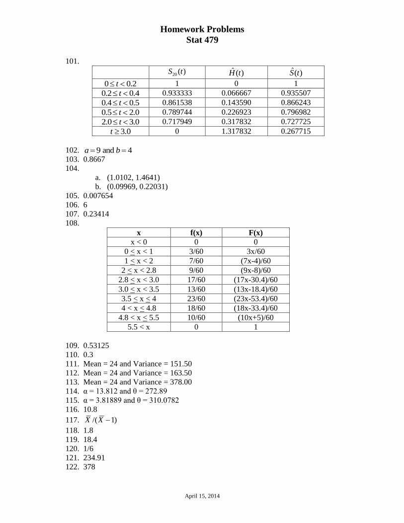
101.
20 ( )S t ˆ ( )H t ˆ( )S t
0 0.2t 1 0 1
0.2 0.4t 0.933333 0.066667 0.935507
0.4 0.5t 0.861538 0.143590 0.866243
0.5 2.0t 0.789744 0.226923 0.796982
2.0 3.0t 0.717949 0.317832 0.727725
3.0t 0 1.317832 0.267715
102. 9 and 4a b
103. 0.8667
104.
a. (1.0102, 1.4641)
b. (0.09969, 0.22031)
105. 0.007654
106. 6
107. 0.23414
108.
x f(x) F(x)
x < 0 0 0
0 < x < 1 3/60 3x/60
1 < x < 2 7/60 (7x-4)/60
2 < x < 2.8 9/60 (9x-8)/60
2.8 < x < 3.0 17/60 (17x-30.4)/60
3.0 < x < 3.5 13/60 (13x-18.4)/60
3.5 < x < 4 23/60 (23x-53.4)/60
4 < x < 4.8 18/60 (18x-33.4)/60
4.8 < x < 5.5 10/60 (10x+5)/60
5.5 < x 0 1
109. 0.53125
110. 0.3
111. Mean = 24 and Variance = 151.50
112. Mean = 24 and Variance = 163.50
113. Mean = 24 and Variance = 378.00
114. α = 13.812 and θ = 272.89
115. α = 3.81889 and θ = 310.0782
116. 10.8
117. )1/( XX
118. 1.8
119. 18.4
120. 1/6
121. 234.91
122. 378
Homework Problems
Stat 479
April 15, 2014
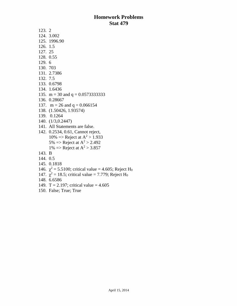
123. 2
124. 3.002
125. 1996.90
126. 1.5
127. 25
128. 0.55
129. 6
130. 703
131. 2.7386
132. 7.5
133. 0.6798
134. 1.6436
135. m = 30 and q = 0.0573333333
136. 0.28667
137. m = 26 and q = 0.066154
138. (1.50426, 1.93574)
139. 0.1264
140. (1/3,0.2447)
141. All Statements are false.
142. 0.2534, 0.61, Cannot reject,
10% => Reject at A2 > 1.933
5% => Reject at A2 > 2.492
1% => Reject at A2 > 3.857
143. B
144. 0.5
145. 0.1818
146. χ2 = 5.5100; critical value = 4.605; Reject H0
147. χ2 = 18.5; critical value = 7.779; Reject H0
148. 6.6586
149. T = 2.197; critical value = 4.605
150. False; True; True

Homework Problems
Stat 479
April 15, 2014
151. 714.42, 2.4, 15
152. 1.6
153. 2
154. 1105.36
155. 14,400
156. 630.79
157. 4
158. 4 8/9
159. C only


![Homework Problems Stat 479jbeckley/WD/STAT 479/… · · 2014-02-20Homework Problems Stat 479 February 19, 2014 Chapter 2 ... For the Pareto distribution, determine E[X], Var(X),](https://static.fdocuments.in/doc/165x107/5b03325e7f8b9a2e228c0b99/homework-problems-stat-479-jbeckleywdstat-4792014-02-20homework-problems-stat.jpg)