Homework 3: Neural Network

1 Deep Learning: a minimal case study (5 pts)

Like any machine learning methods, neural networks have two modes: inference/prediction

and learning/training. They are implemented as forward propagation and backward propagation

(backprop for short).

Get the starter code from this GitHub repo. If you’re new to GitHub, there are some guides here.

Star the repo to get notified of changes (e.g., bug fixes) and follow the instructions to clone it to

your machine. “fnn.py” contains a minimal implementation of multi-layer feedforward neural

network. The main class is FNN that folds a list of layers and defines the high level iterative process

for forward and backward propagation. The class Layer implements each layer in the neural

network. The class GradientDescentOptimizer implements an optimizer for training the neural

network. The utility functions at the end implement different activation functions, loss functions

and their gradients. Read through “fnn.py” to get an overview of the implementation. We are

using stochastic gradient descent instead of minibatch gradient descent, see this video to learn

more.

Complete the following steps to finish part 1:

First, read this note on intuition and implementation tips for Backpropagation. Backprop in

practice: Staged computation and Gradients for vectorized operations sections are especially

helpful with good examples and practical tips.

Then, complete the code in the following two parts.

1. Forward propagation: the core of inference/prediction in NN.

In this part, you need to complete the forward method in class Layer in “fnn.py” (search for

“Question 1” to see the instructions). (2 lines of code, 1pt)

2. Backpropagation: the core of learning/training in NN.

In this part, you need to complete the backward method in class Layer in “fnn.py” (search

for “Question” to see the instructions). (4 lines of code 3 pts)

To test your implementation, first download the MNIST dataset by running

python get_mnist_data.py

Then run

python test_fnn.py

There are two tests (test_forwardprop and test_backprop). When your implementation passes

both of them, run

python mnist_experiment.py

to train a small deep neural network with 1 hidden layer (containing 128 sigmoid units) for

handwritten digit recognition using MNIST dataset. The accuracy should be around 99% on

training set and around 97% on validation and test set.

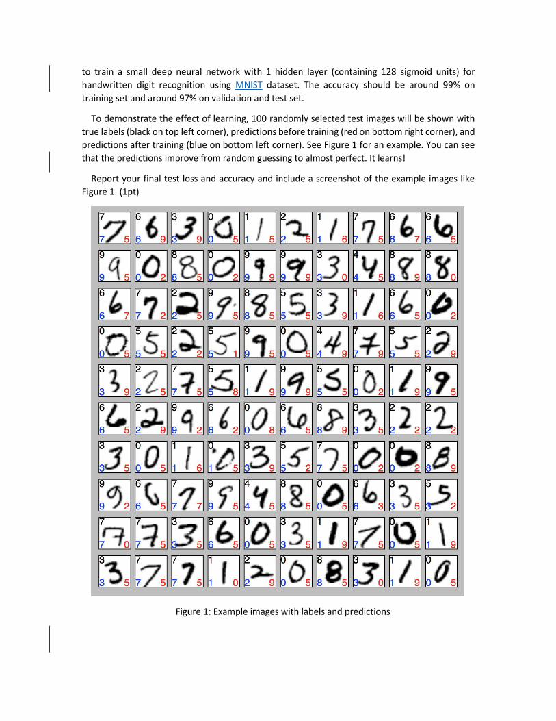
To demonstrate the effect of learning, 100 randomly selected test images will be shown with

true labels (black on top left corner), predictions before training (red on bottom right corner), and

predictions after training (blue on bottom left corner). See Figure 1 for an example. You can see

that the predictions improve from random guessing to almost perfect. It learns!

Report your final test loss and accuracy and include a screenshot of the example images like

Figure 1. (1pt)

Figure 1: Example images with labels and predictions

2 Char-RNN in TensorFlow (5pts)

A char-RNN is a Recurrent Neural Network for Character-level language modeling. Read this fun

blog to learn more about it. We will play with a TensorFlow implementation of this model for

training and sampling.

Setup: in this part, instead of writing your own code and running experiments on your own

laptop, you will use existing open source code from Github on a cloud computing platform (Google

Cloud Platform). Follow the following instructions to setup your GCP machine and github repo.

(1) Get a voucher. We will be giving out $50 vouchers in class on the week of May 14th. An

alternative is to sign up for a free trial of the Google Cloud Platform using your own credit

card.

(2) Log in your own gmail account. https://www.google.com/gmail/ Please note that

Northwestern restricts the Google Cloud Platform on our @u.northwestern.edu accounts,

so do not use your u.northwestern.edu!!! Otherwise, you will lose your $50 voucher!

(3) Make sure that your current gmail account ends with gmail.com

(4) Now, input the code at the bottom of your voucher at: bit.ly/gcp-redeem. Click ‘accept

and continue’ at the bottom of the webpage. You will see a screenshot like this:

(5) Go to https://console.cloud.google.com/cloud-resource-manager and create a new

project. Enter the homepage of your new project. You should be able to see a screenshot

like this.

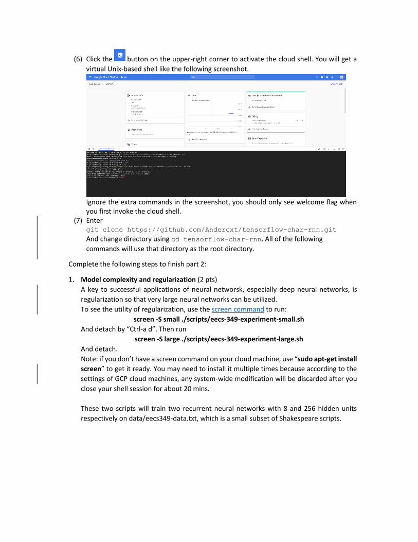
(6) Click the button on the upper-right corner to activate the cloud shell. You will get a

virtual Unix-based shell like the following screenshot.

Ignore the extra commands in the screenshot, you should only see welcome flag when you first invoke the cloud shell.

(7) Enter git clone https://github.com/Andercxt/tensorflow-char-rnn.git

And change directory using cd tensorflow-char-rnn. All of the following

commands will use that directory as the root directory.

Complete the following steps to finish part 2:

1. Model complexity and regularization (2 pts)

A key to successful applications of neural networsk, especially deep neural networks, is

regularization so that very large neural networks can be utilized.

To see the utility of regularization, use the screen command to run:

screen -S small ./scripts/eecs-349-experiment-small.sh

And detach by “Ctrl-a d”. Then run

screen -S large ./scripts/eecs-349-experiment-large.sh

And detach.

Note: if you don’t have a screen command on your cloud machine, use “sudo apt-get install

screen” to get it ready. You may need to install it multiple times because according to the

settings of GCP cloud machines, any system-wide modification will be discarded after you

close your shell session for about 20 mins.

These two scripts will train two recurrent neural networks with 8 and 256 hidden units

respectively on data/eecs349-data.txt, which is a small subset of Shakespeare scripts.

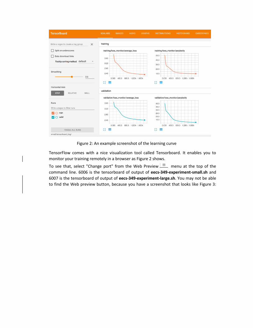
Figure 2: An example screenshot of the learning curve

TensorFlow comes with a nice visualization tool called Tensorboard. It enables you to

monitor your training remotely in a browser as Figure 2 shows.

To see that, select "Change port" from the Web Preview menu at the top of the

command line. 6006 is the tensorboard of output of eecs-349-experiment-small.sh and

6007 is the tensorboard of output of eecs-349-experiment-large.sh. You may not be able

to find the Web preview button, because you have a screenshot that looks like Figure 3:

Figure 3 The situation where you can’t find Web Preview Menu button

This is because of a CSS website bug in the Google Cloud Platform website.

You just need to hide the tool menu on the left side by clicking once on the top-left

corner of the GCP website, and then there should be no problem.

Note: if you want to see your own results in tensorboard for your experiments in Part 3

Have fun, enter the following command:

tensorboard --logdir=your-output-dir --port=your-port

Replace your-output-dir and your-port with your output directory and your port.

Include screenshots of the learning curves as in Figure 2. And answer the questions: what

is the difference between the learning curves of the two recurrent neural networks, and

why? (1pt)

Dropout is an effective way to regularize deep neural network.

Make a copy of eecs-349-experiment-large.sh and modify it to use dropout=0.1,0.3,0.5.

Include screenshots of the learning curves. Report the final validation and test perplexities

(saved in the best_valid_ppl and test_ppl fields in result.json in your output folder, you

may find the cat command handy). What is the difference between their learning curves

and why? (1pt)

Note: this example is just for illustration purposes. The dataset is too small to train a good

model. Usually dropout has a much larger effect in real applications of very large neural

networks.

2. Sampling (2pts)

A fun aspect of language modeling is that, after training a model, you can use it to generate

samples. A model pretrained on Shakespeare scripts is included in the

pretrained_shakespeare folder in the repo.

To get an example sample, run

python sample.py --init_dir=pretrained_shakespeare \

--length=1000 \

--temperature=0.5 \

--start_text="HAMLET:"

The secret sauce to good samples is a hyperparameter called temperature. It changes the

shape of the output probability distribution from Softmax function. The original distribution

is

𝑝(𝑐𝑖) =𝑒𝑠𝑖

∑ 𝑒𝑠𝑖𝑛𝑖=1

After adding temperature, it becomes

𝑝(𝑐𝑖) =𝑒𝑠𝑖𝑡

∑ 𝑒𝑠𝑖𝑡𝑛

𝑖=1

where p(ci) is the probability to output the i-th character, and si is the score (the neural

network output) for the i-th character.

The temperature is defaulted to be 1.0. Usually value smaller than 1.0, for example 0.5,

gives you more reasonable samples. But to get a feeling of the effect of low and high

temperature, try sampling with temperature=0.01 and 5.0, how are the samples different

from the previous one (temperature=0.5) and why? (think about how the temperature

would change the shape of the distribution)

3. Have fun (1pt).

Now is the fun part, collect your own dataset (a file of characters, usually TXT files, for

example, your favorite novel, Taylor Swift’s lyrics, etc) and train Char-RNN on it and get

some fun samples. Note that you need to know the encoding (default to “utf-8”) of your

file and use the “encoding” argument of “train.py”. Here’s a list of encodings you can try if

you are not sure.

To get a good result, the dataset should be large enough (at least more than 10 KB and a

good one should be more than 1 MB). Your usually need larger model, and train for a long

time (around 3 hrs using default settings on 1MB). Use tensorboard to monitor your training.

Start with the default settings like

python train.py --data_file=path/to/your-own-data \ --encoding="your-file-encoding" \

--batch_size=100 \ --output_dir=your-output-dir

then tune the hyperparameters like hidden size, number of layers, number of unrollings

and dropout rate to get lower perplexity.

Tune the temperature parameter to generate some fun samples from your trained model.

Use start_text to warm up your Char-RNN and use seed to make your samples replicable.

python sample.py --init_dir=your-output-dir \ --length=1000 \

--seed=your-integer-random-seed \ --start_text="your-start-text" \

--temperature=0.5 Describe the dataset you used for training. Include screenshots (Figure 2) of your learning

curves, the result.json in your output folder, and some of your favorite samples. We will

share some of the funniest samples in the class :)

3 Groups

1. For part 1, you can discuss in groups, but the coding should be done individually.

2. For part 2, you can work in groups of 2-3, but each needs to submit a write-up separately.

It is recommended that at least one of the group members should be familiar with Linux

command line.

4 What to submit

A zip file containing the following:

1. The original folder “part-1” with your modified “fnn.py”

2. A PDF file including the answers to your questions, screenshots, the content of the

“results.json” files and your favorite samples.

3. Include a list of your group members and who did what in the PDF.