Neural Networks 19 (2006) 734–743www.elsevier.com/locate/neunet

2006 Special Issue

Homeostatic synaptic scaling in self-organizing maps

Thomas J. Sullivana,∗, Virginia R. de Sab

a Department of Electrical Engineering, UC San Diego, 9500 Gilman Dr. MC 0515, 92093 La Jolla, CA, United Statesb Department of Cognitive Science, UC San Diego, La Jolla, CA, United States

Abstract

Various forms of the self-organizing map (SOM) have been proposed as models of cortical development [Choe Y., Miikkulainen R., (2004).Contour integration and segmentation with self-organized lateral connections. Biological Cybernetics, 90, 75–88; Kohonen T., (2001). Self-organizing maps (3rd ed.). Springer; Sirosh J., Miikkulainen R., (1997). Topographic receptive fields and patterned lateral interaction in aself-organizing model of the primary visual cortex. Neural Computation, 9(3), 577–594]. Typically, these models use weight normalization tocontain the weight growth associated with Hebbian learning. A more plausible mechanism for controlling the Hebbian process has recentlyemerged. Turrigiano and Nelson [Turrigiano G.G., Nelson S.B., (2004). Homeostatic plasticity in the developing nervous system. Nature ReviewsNeuroscience, 5, 97–107] have shown that neurons in the cortex actively maintain an average firing rate by scaling their incoming weights. Inthis work, it is shown that this type of homeostatic synaptic scaling can replace the common, but unsupported, standard weight normalization.Organized maps still form and the output neurons are able to maintain an unsaturated firing rate, even in the face of large-scale cell proliferationor die-off. In addition, it is shown that in some cases synaptic scaling leads to networks that more accurately reflect the probability distribution ofthe input data.c© 2006 Elsevier Ltd. All rights reserved.

Keywords: Self-organizing map; Homeostasis; Weight normalization; Synaptic scaling

1. Introduction

The self-organizing map (SOM), in its various forms,has been a useful model of cortical development (Choe &Miikkulainen, 2004; Kohonen, 2001; Obermayer, Blasdel, &Schulten, 1992; Sirosh & Miikkulainen, 1997). Sirosh andMiikkulainen (1997) showed the simultaneous development ofreceptive field properties and lateral interactions in a realisticmodel. The usefulness of the developed lateral connectionswas shown by Choe and Miikkulainen (2004) for contourintegration and segmentation. It is this lateral connectivity thatensures the neighboring neurons come to respond to similarstimuli and form a good map.

In these models, Hebbian learning is used to strengthenassociations between stimuli and winning neurons. This typeof associative learning has been well documented in theexperimental literature (Bi & Poo, 2001; Bliss & Lomo,

∗ Corresponding author.E-mail addresses: tom@sullivan.to (T.J. Sullivan), desa@cogsci.ucsd.edu

(V.R. de Sa).

0893-6080/$ - see front matter c© 2006 Elsevier Ltd. All rights reserved.doi:10.1016/j.neunet.2006.05.006

1973), but our understanding has remained incomplete. It iswell known that the most straightforward implementationsof Hebbian learning lead to unconstrained weight growth.To counteract this problem, typical SOM algorithms useweight normalization: after each learning iteration all theweights converging onto a neuron are divided by the sumof the incoming weights (or the square root of the sum ofthe squared weights). It has been argued that this type ofweight normalization is biologically plausible. For example, aneuron might have a finite resource necessary for maintainingincoming synapses. This might keep an upper limit on thetotal summed size of the incoming synapses. While this soundswithin the realm of biological possibility, and is obviouslyhelpful in keeping Hebbian learning in check, little evidencefrom the experimental literature is available for support.

More plausible mechanisms for controlling the Hebbianprocess based on maintaining an average output firing ratehave recently emerged. Two different types of these internalmechanisms have been found. One type controls the intrinsicexcitability of the neuron (reviewed by Zhang and Linden(2003)). The molecular causes underlying this mechanism are

T.J. Sullivan, V.R. de Sa / Neural Networks 19 (2006) 734–743 735

still being investigated, but some of the behavior has beendocumented. In a typical experiment, a neuron would be excitedrepeatedly at high frequency. Then the output firing rate wouldbe measured when current is injected. The intrinsic excitability(the ratio of firing rate to injected current) is higher after thestimulation. This makes the neuron even more sensitive to itsinputs.

Two models have proposed that neurons modify theirexcitability to maintain a high rate of information transfer. Inthe first of these models (Stemmler & Koch, 1999), individualneurons change their ion channel conductances in order tomatch an input distribution. The neurons are able to maintainhigh information rates in response to a variety of distributions.The second model (Triesch, 2004) proposes that neurons adjusttheir output nonlinearities to maximize information transfer.There it is assumed that the neuron can keep track of its averagefiring rate and average variance of firing rate. Given this limitedinformation, it does the best it can by adjusting the slope andoffset of an output sigmoid function.

In the second type of internal neuronal mechanism it wasshown (Maffei, Nelson, & Turrigiano, 2004; Turrigiano, Leslie,Desai, Rutherford, & Nelson, 1998; Turrigiano & Nelson,2004) that neurons in the cortex actively maintain an averagefiring rate by scaling their incoming weights. The mechanismhas been examined in cultures and in other experimentsusing in vivo visual deprivation. It has been shown that theincoming synapses are altered by a multiplicative factor, whichpresumably preserves the relative strengths of the synapses.The underlying mechanisms are not yet known, but thereis ongoing research looking at intracellular chemical factorssuch as calcium and brain-derived neurotrophic factor (BDNF)(Turrigiano & Nelson, 2004). The levels of these factors arerelated to firing rates, so integrating them over time could leadto an estimate of average firing rate and produce a chemicalsignal for synaptic change. Another interesting finding is that aneuron with high average firing rate will decrease the strengthof incoming excitatory synapses, but increase the strength ofincoming inhibitory neurons (Maffei et al., 2004), thus alteringthe excitatory/inhibitory balance.

Homeostatic mechanisms have been implemented in twomodels. In one study, the molecular underpinnings ofhomeostasis were explored (Yeung, Shouval, Blais, & Cooper,2004). It was suggested that LTP, LTD, and synaptichomeostatic scaling are all related through intracellular calciumlevels. The homeostatic mechanism may influence the levelof calcium, thereby changing under what conditions LTP andLTD are induced (since calcium levels play a major rolein LTP and LTD). The other model concerns a particularclass of associative memories (Chechik, Meilijson, & Ruppin,2001). It is shown that the storage capacity can be increasedif the neuron’s weights are controlled with either weightnormalization or homeostatic synaptic scaling.

There have also been attempts to change neuron thresholdswithin neural networks. One network that was described (Horn& Usher, 1989) was a Hopfield network with neurons that werealways producing one of two possible outputs (+1 or −1). Theneuronal thresholds for determining which state to be in, acting

on the total amount of input activation, was adjusted accordingto the recent activation. They reported that interesting periodicdynamics emerged. Another adjustable threshold network(Gorchetchnikov, 2000) was a winner-take-all associativememory. In that work, the thresholds on output sigmoidfunctions were adjusted. It was shown that on problems likeXOR classification, the network would learn the appropriatemapping faster than without an adjustable threshold. Whilethese approaches are computationally interesting, there is notyet evidence that neurons adjust their threshold based on theiraverage firing rate.

It has previously been suggested that homeostatic synapticscaling might form a basis for keeping Hebbian learningin check (Miller, 1996; Turrigiano & Nelson, 2004). Thispossibility is explored here. It may very well be that thismechanism is one of several that constrain synapse strength,but it is examined here in isolation to get a better understandingof its capability.

2. Architecture with homeostatic synaptic scaling

The SOM model is trained with a series of episodes inwhich randomly selected input vectors are presented. At eachstep, the input vector, Ex , is first multiplied by the feedforwardweights, WF F . In order to get the self-organizing map effect,this feedforward activity is then multiplied by a set of lateralconnections, Wlat. The patterns of weights that the neurons sendout laterally are identical to a preset prototype, so multiplyingby Wlat is equivalent to taking a convolution with a kernel, g.

Ey f f = WF F Ex (1)

Ey = f [g ∗ Ey f f ]. (2)

Here f [a] = max(0, a) and g is preset to a Mexican hat shape.These steps are similar to those proposed recently by Kohonen(2005, 2006). In that case, though, g took on a different form, asdid the function f . Also, multiplying by a Mexican hat kernelwas explored by Kohonen (1982), but in that work the kernelwas applied iteratively until the neural activities were no longerchanging. This is a time-consuming process so is not pursuedhere.

In this version the lateral connections are not updated withlearning, but after the output activity is set the feedforwardweights are updated with a Hebbian learning rule:

w̃ti j = wt−1

i j + αx tj yt

i (3)

α is the Hebbian learning rate, x j is the presynaptic activityand yi is the postsynaptic activity. w̃i j is simply a weight valueafter Hebbian learning, but before weight normalization. Thesuperscripts t and t−1 are added here to index the mathematicalprocessing steps in this discrete-time model. The superscript tis used to indicate a current value, while t − 1 indicates thatthe value is the result of calculations performed in the previoustime step.

It is this type of Hebbian learning rule that would normallygive problems. Since each update is positive, there is nothingto limit the growth of the weights. Normally, a weight

736 T.J. Sullivan, V.R. de Sa / Neural Networks 19 (2006) 734–743

normalization is used that is based on the sum of the magnitudesof the weights coming into each neuron. In our case, we willnormalize the weights with a value based on the recent activityof the neuron:

wti j =

w̃ti j

ActivityNormti

(4)

ActivityNormti = 1 + βN

(At−1

avg,i − Atarget

Atarget

). (5)

Here, Atarget is the internally defined preferred activity levelfor the neurons, Aavg,i is the average of recent activity forneuron i , and βN is the homeostatic learning rate. This modelassumes that some intracellular chemical, something activatedby calcium for example, is integrated over the recent pastand is related to the average firing rate. If the target level ofthis chemical is exceeded, the incoming synapse sizes willbe decreased multiplicatively. If the target is not achieved,the synapses will be increased. Since the underlying relevantchemicals and their dynamics are not yet known, we insteaduse the average firing rate and firing rate target value directly incomputing ActivityNorm.

In the model, each neuron keeps track of its average outputfiring rate, At

avg,i , with a running average over the recent past.

Atavg,i = βC yt

i + (1 − βC )At−1avg,i . (6)

Here, βC controls the time window over which the neuron’sfiring rate is averaged.

This is a local computation, in the sense that each neuronkeeps track of its own average firing rate. If this average,or difference from the target, is expressed as an internallevel of some chemical all the synapses would conceivablyhave access to that information. Using the At

avg,i and Atargetvalues directly avoids modelling the concentrations of unknownchemicals, but as more details become available throughexperiments, the model can become more explicit. It isinteresting to note that there are different degrees to the localityof information. There is (1) information local to individualsynapses, (2) information local to individual neurons, and (3)global information (information exchanged across neurons).The standard weight normalization and the new homeostaticmechanism both belong to the second class. One difference,however, is the nature of the information exchange inside theneuron. In the standard weight normalization case, a synapsewould communicate its magnitude to the soma, which wouldin response change all the other synapse strengths. In the newmethod the communication is one way: the soma decides, basedon the average firing rate, whether all the synapses should beincreased or decreased.

3. Simulation results

Self-organizing maps were simulated using the synapticscaling described with the previous equations. The input vectorsused in these simulations are specified by a 1-D Gaussianshape (standard deviation σ of 15 units) and are presented

one per episode. For each episode, the input Gaussian iscentered on one of the input units selected at random. Theinput locations are drawn from a uniform distribution forthe experiments described in Sections 3.1 and 3.2. Otherprobability distributions are used in Section 3.3 as described.A typical training session lasts for 100,000 episodes. Ateach step Eqs. (1) and (2) are used to determine the neuronactivities using the randomly selected input vector, Ex . Afterthe neuron activities are determined the Hebbian weight updateof Eq. (3) is applied to every feedforward weight, as is thesynaptic scaling rule of Eq. (4). Also, during each episode theActivityNorm value and the Aavg value must be updated for eachneuron using Eqs. (5) and (6), respectively. In other work, weshow how to find the range of effective learning rate parameters(Sullivan & de Sa, 2006), so only values in this range are used.In all the simulations described here α = 8.3 × 10−4, βN =

3.3 × 10−4, βC = 3.3 × 10−5, and Atarget = 0.1 Hz.

3.1. Homeostasis and map formation

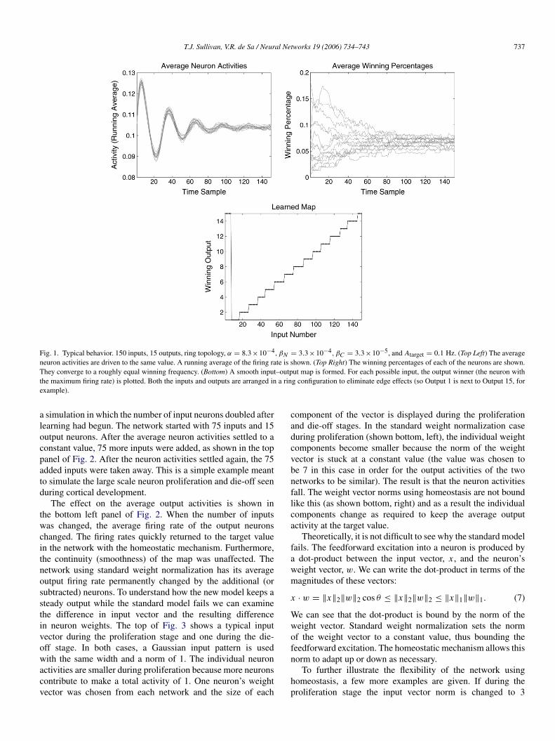
In order to verify proper formation of a map, a networkwas created with 150 inputs and 15 outputs. Both the inputsand outputs are arranged in a ring configuration to eliminateedge effects. The input vectors are specified by a 1-D Gaussianshape (standard deviation σ of 15 units). The input Gaussianis centered on one of the input units, selected uniformly atrandom. Plots of typical network behavior are shown in Fig. 1.In the top left plot, the average firing rate of the output neuronsis shown. As the simulation progresses the average neuronfiring rate approaches Atarget. For each input, if we view themost active output neuron as the winner, then we can keep trackof the neurons’ winning percentages. The top right plot showsthese winning percentages for all the output neurons. It can beseen that they approach a roughly equal probability of winning.The bottom plot shows an input–output map that has formedafter training has ended. To obtain this plot, every possible inputwas presented to the network, one at a time. The winning outputneuron (the one with the highest output rate) was then recordedfor each input. The input number is shown on the x axis, andthe corresponding winning output is plotted. This is a goodmap since similar inputs (inputs whose center is located onneighboring input units) correspond to nearby winning outputunits.

3.2. Synapse proliferation

Homeostatic mechanisms that maintain a steady outputfiring rate may play a particularly important role duringdevelopment. As many neurons and synapses are added andpruned away, the total amount of input drive to a neuron willchange dramatically. In order to avoid having a saturated firingrate, neurons must regulate themselves. Additionally, duringnormal functioning in a hierarchical system such as the visualcortex, one area’s output is another’s input. For the benefit ofhigher areas, it may be important for neurons to maintain aconsistent firing rate level.

In order to test the ability of homeostatic synaptic scaling towithstand dramatic changes in network architecture, we created

T.J. Sullivan, V.R. de Sa / Neural Networks 19 (2006) 734–743 737

Fig. 1. Typical behavior. 150 inputs, 15 outputs, ring topology, α = 8.3×10−4, βN = 3.3×10−4, βC = 3.3×10−5, and Atarget = 0.1 Hz. (Top Left) The averageneuron activities are driven to the same value. A running average of the firing rate is shown. (Top Right) The winning percentages of each of the neurons are shown.They converge to a roughly equal winning frequency. (Bottom) A smooth input–output map is formed. For each possible input, the output winner (the neuron withthe maximum firing rate) is plotted. Both the inputs and outputs are arranged in a ring configuration to eliminate edge effects (so Output 1 is next to Output 15, forexample).

a simulation in which the number of input neurons doubled afterlearning had begun. The network started with 75 inputs and 15output neurons. After the average neuron activities settled to aconstant value, 75 more inputs were added, as shown in the toppanel of Fig. 2. After the neuron activities settled again, the 75added inputs were taken away. This is a simple example meantto simulate the large scale neuron proliferation and die-off seenduring cortical development.

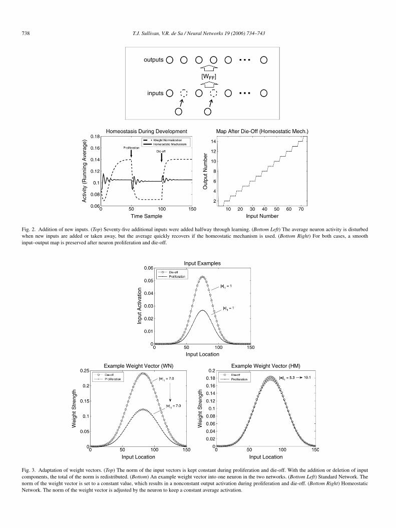
The effect on the average output activities is shown inthe bottom left panel of Fig. 2. When the number of inputswas changed, the average firing rate of the output neuronschanged. The firing rates quickly returned to the target valuein the network with the homeostatic mechanism. Furthermore,the continuity (smoothness) of the map was unaffected. Thenetwork using standard weight normalization has its averageoutput firing rate permanently changed by the additional (orsubtracted) neurons. To understand how the new model keeps asteady output while the standard model fails we can examinethe difference in input vector and the resulting differencein neuron weights. The top of Fig. 3 shows a typical inputvector during the proliferation stage and one during the die-off stage. In both cases, a Gaussian input pattern is usedwith the same width and a norm of 1. The individual neuronactivities are smaller during proliferation because more neuronscontribute to make a total activity of 1. One neuron’s weightvector was chosen from each network and the size of each

component of the vector is displayed during the proliferationand die-off stages. In the standard weight normalization caseduring proliferation (shown bottom, left), the individual weightcomponents become smaller because the norm of the weightvector is stuck at a constant value (the value was chosen tobe 7 in this case in order for the output activities of the twonetworks to be similar). The result is that the neuron activitiesfall. The weight vector norms using homeostasis are not boundlike this (as shown bottom, right) and as a result the individualcomponents change as required to keep the average outputactivity at the target value.

Theoretically, it is not difficult to see why the standard modelfails. The feedforward excitation into a neuron is produced bya dot-product between the input vector, x , and the neuron’sweight vector, w. We can write the dot-product in terms of themagnitudes of these vectors:

x · w = ‖x‖2‖w‖2 cos θ ≤ ‖x‖2‖w‖2 ≤ ‖x‖1‖w‖1. (7)

We can see that the dot-product is bound by the norm of theweight vector. Standard weight normalization sets the normof the weight vector to a constant value, thus bounding thefeedforward excitation. The homeostatic mechanism allows thisnorm to adapt up or down as necessary.

To further illustrate the flexibility of the network usinghomeostasis, a few more examples are given. If during theproliferation stage the input vector norm is changed to 3

738 T.J. Sullivan, V.R. de Sa / Neural Networks 19 (2006) 734–743

Fig. 2. Addition of new inputs. (Top) Seventy-five additional inputs were added halfway through learning. (Bottom Left) The average neuron activity is disturbedwhen new inputs are added or taken away, but the average quickly recovers if the homeostatic mechanism is used. (Bottom Right) For both cases, a smoothinput–output map is preserved after neuron proliferation and die-off.

Fig. 3. Adaptation of weight vectors. (Top) The norm of the input vectors is kept constant during proliferation and die-off. With the addition or deletion of inputcomponents, the total of the norm is redistributed. (Bottom) An example weight vector into one neuron in the two networks. (Bottom Left) Standard Network. Thenorm of the weight vector is set to a constant value, which results in a nonconstant output activation during proliferation and die-off. (Bottom Right) HomeostaticNetwork. The norm of the weight vector is adjusted by the neuron to keep a constant average activation.

T.J. Sullivan, V.R. de Sa / Neural Networks 19 (2006) 734–743 739

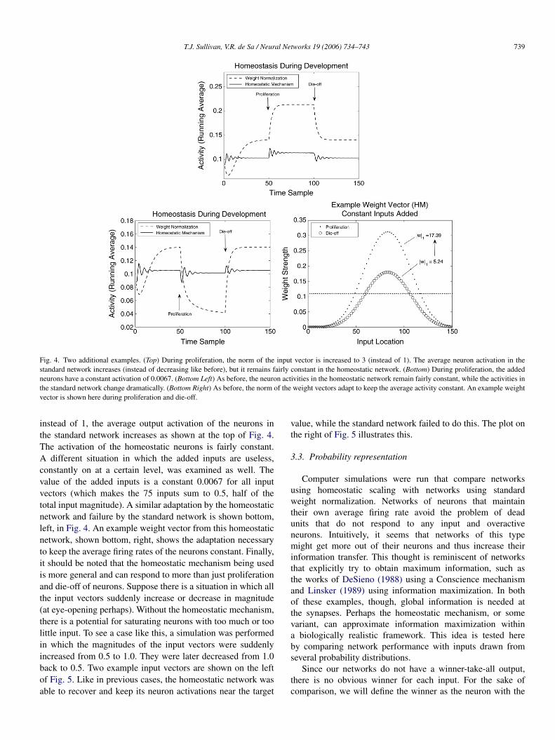
Fig. 4. Two additional examples. (Top) During proliferation, the norm of the input vector is increased to 3 (instead of 1). The average neuron activation in thestandard network increases (instead of decreasing like before), but it remains fairly constant in the homeostatic network. (Bottom) During proliferation, the addedneurons have a constant activation of 0.0067. (Bottom Left) As before, the neuron activities in the homeostatic network remain fairly constant, while the activities inthe standard network change dramatically. (Bottom Right) As before, the norm of the weight vectors adapt to keep the average activity constant. An example weightvector is shown here during proliferation and die-off.

instead of 1, the average output activation of the neurons inthe standard network increases as shown at the top of Fig. 4.The activation of the homeostatic neurons is fairly constant.A different situation in which the added inputs are useless,constantly on at a certain level, was examined as well. Thevalue of the added inputs is a constant 0.0067 for all inputvectors (which makes the 75 inputs sum to 0.5, half of thetotal input magnitude). A similar adaptation by the homeostaticnetwork and failure by the standard network is shown bottom,left, in Fig. 4. An example weight vector from this homeostaticnetwork, shown bottom, right, shows the adaptation necessaryto keep the average firing rates of the neurons constant. Finally,it should be noted that the homeostatic mechanism being usedis more general and can respond to more than just proliferationand die-off of neurons. Suppose there is a situation in which allthe input vectors suddenly increase or decrease in magnitude(at eye-opening perhaps). Without the homeostatic mechanism,there is a potential for saturating neurons with too much or toolittle input. To see a case like this, a simulation was performedin which the magnitudes of the input vectors were suddenlyincreased from 0.5 to 1.0. They were later decreased from 1.0back to 0.5. Two example input vectors are shown on the leftof Fig. 5. Like in previous cases, the homeostatic network wasable to recover and keep its neuron activations near the target

value, while the standard network failed to do this. The plot onthe right of Fig. 5 illustrates this.

3.3. Probability representation

Computer simulations were run that compare networksusing homeostatic scaling with networks using standardweight normalization. Networks of neurons that maintaintheir own average firing rate avoid the problem of deadunits that do not respond to any input and overactiveneurons. Intuitively, it seems that networks of this typemight get more out of their neurons and thus increase theirinformation transfer. This thought is reminiscent of networksthat explicitly try to obtain maximum information, such asthe works of DeSieno (1988) using a Conscience mechanismand Linsker (1989) using information maximization. In bothof these examples, though, global information is needed atthe synapses. Perhaps the homeostatic mechanism, or somevariant, can approximate information maximization withina biologically realistic framework. This idea is tested hereby comparing network performance with inputs drawn fromseveral probability distributions.

Since our networks do not have a winner-take-all output,there is no obvious winner for each input. For the sake ofcomparison, we will define the winner as the neuron with the

740 T.J. Sullivan, V.R. de Sa / Neural Networks 19 (2006) 734–743

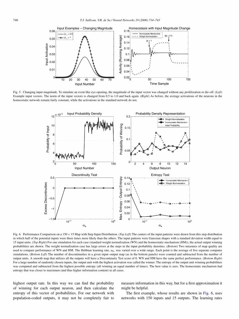
Fig. 5. Changing input magnitude. To simulate an event like eye-opening, the magnitude of the input vector was changed without any proliferation or die-off. (Left)Example input vectors. The norm of the input vectors is changed from 0.5 to 1.0 and back again. (Right) As before, the average activations of the neurons in thehomeostatic network remain fairly constant, while the activations in the standard network do not.

Fig. 6. Performance Comparison on a 150×15 Map with Step Input Distribution. (Top Left) The centers of the input patterns were drawn from this step distributionin which half of the potential inputs were three times more likely than the others. The input patterns were Gaussian shapes with a standard deviation width equal to15 input units. (Top Right) For one simulation for each case (standard weight normalization (WN) and the homeostatic mechanism (HM)), the actual output winningprobabilities are shown. The weight normalization case has large errors at the steps in the input probability densities. (Bottom) Two measures of map quality areused to compare performance of WN and HM. The Hebbian learning rate, αk , was varied over a wide range. Each point is the average of five separate computersimulations. (Bottom Left) The number of discontinuities in a given input–output map (as in the bottom panels) were counted and subtracted from the number ofoutput units. A smooth map that utilizes all the outputs will have a Discontinuity Test score of 0. WN and HM have the same perfect performance. (Bottom Right)For a large number of randomly chosen inputs, the output unit with the highest activation was called the winner. The entropy of the output unit winning probabilitieswas computed and subtracted from the highest possible entropy (all winning an equal number of times). The best value is zero. The homeostatic mechanism hadentropy that was closer to maximum (and thus higher information content) in all cases.

highest output rate. In this way we can find the probabilityof winning for each output neuron, and then calculate theentropy of this vector of probabilities. For our network withpopulation-coded outputs, it may not be completely fair to

measure information in this way, but for a first approximation itmight be helpful.

The first example, whose results are shown in Fig. 6, usesnetworks with 150 inputs and 15 outputs. The learning rates

T.J. Sullivan, V.R. de Sa / Neural Networks 19 (2006) 734–743 741

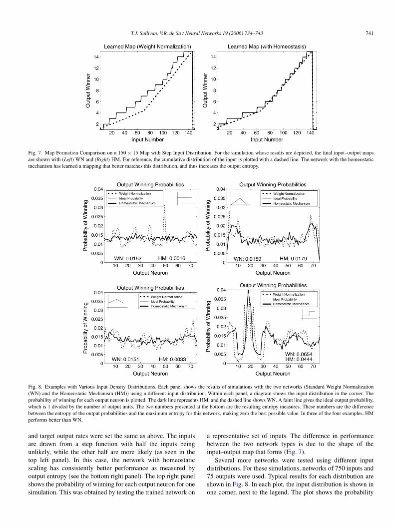
Fig. 7. Map Formation Comparison on a 150 × 15 Map with Step Input Distribution. For the simulation whose results are depicted, the final input–output mapsare shown with (Left) WN and (Right) HM. For reference, the cumulative distribution of the input is plotted with a dashed line. The network with the homeostaticmechanism has learned a mapping that better matches this distribution, and thus increases the output entropy.

Fig. 8. Examples with Various Input Density Distributions. Each panel shows the results of simulations with the two networks (Standard Weight Normalization(WN) and the Homeostatic Mechanism (HM)) using a different input distribution. Within each panel, a diagram shows the input distribution in the corner. Theprobability of winning for each output neuron is plotted. The dark line represents HM, and the dashed line shows WN. A faint line gives the ideal output probability,which is 1 divided by the number of output units. The two numbers presented at the bottom are the resulting entropy measures. These numbers are the differencebetween the entropy of the output probabilities and the maximum entropy for this network, making zero the best possible value. In three of the four examples, HMperforms better than WN.

and target output rates were set the same as above. The inputsare drawn from a step function with half the inputs beingunlikely, while the other half are more likely (as seen in thetop left panel). In this case, the network with homeostaticscaling has consistently better performance as measured byoutput entropy (see the bottom right panel). The top right panelshows the probability of winning for each output neuron for onesimulation. This was obtained by testing the trained network on

a representative set of inputs. The difference in performancebetween the two network types is due to the shape of theinput–output map that forms (Fig. 7).

Several more networks were tested using different inputdistributions. For these simulations, networks of 750 inputs and75 outputs were used. Typical results for each distribution areshown in Fig. 8. In each plot, the input distribution is shown inone corner, next to the legend. The plot shows the probability

742 T.J. Sullivan, V.R. de Sa / Neural Networks 19 (2006) 734–743

of winning for each output neuron. The dark line representsthe neurons in the network with the homeostatic mechanism,and the dashed line gives the network with standard weightnormalization. A faint line gives the ideal output winningprobability, which is 1 divided by the number of output units.At the bottom of each plot are the resulting entropy measuresfor the two networks, standard weight normalization (WN)and the homeostatic mechanism (HM). These numbers are thedifference between the entropy of the output probabilities andthe maximum entropy for this network, making zero the bestpossible value.

In three out of four cases, the network with the homeostaticmechanism had better performance. The network with standardweight normalization was slightly better in the second case.Interestingly, this ramp-like distribution caused the homeostaticmechanism to converge to a state in which some neurons rarelywon (had the most activation). These output neurons receivedenough activation from neighboring winners that their targetactivity goal was achieved. In other words, all neurons hadsimilar average activities, but some neurons rarely ‘won’. Alsointeresting were the results of the last distribution. This wasthe same input step distribution as was used in the exampleabove. As the network size increased, performance gets worsefor both networks. This is again due to the algorithm optimizingfor average firing rate, not average winning percentage. Thediscrepancy between these measures, especially in the regionsof low probability, should be interesting grounds for futureinvestigation.

We do not fully understand why the homeostatic networkperforms better in these simulations. Our intuition leads us tobelieve that in this network, neurons that are not respondingmuch can make themselves more useful by increasing theiraverage activations. This is not necessarily the same asincreasing a winning percentage, but it may be some sort ofapproximation. We believe that this can be an interesting areafor further investigation and we would benefit by understandingsome theoretical aspects behind this performance.

4. Conclusions

In this work, we have proposed a way to go beyond thestandard weight normalization. This long-used measure hasworked to counteract the unconstrained growth of Hebbianlearning, but there is little evidence from experiments thatjustifies its use. Homeostatic synaptic scaling, on the otherhand, has been seen recently in biological experiments. It hasbeen shown here that using homeostatic synaptic scaling inplace of standard weight normalization still leads to properorganized map formation. In addition, the neurons are ableto maintain their average firing rates at a set point. Thishelps them from becoming saturated as neurons are addedor taken away, as happens during development. Finally, itwas shown that synaptic scaling in some cases leads toa better representation of the input probability distributioncompared with weight normalization. This observation suggeststhe intriguing possibility that this homeostatic mechanism helpsdrive the network to a state of increasing information transfer.

The output entropy was measured using the probabilityof each output neuron having the highest activation. Thismay not be the most natural way to measure informationtransfer in this network, since a population code is used asthe output. Indeed, since the neurons’ goal is to maintain auseful average firing rate, information transfer may not bethe most important measure of performance. These issueswill be addressed in future work. The algorithm will alsobe tested more extensively with two-dimensional input andoutput spaces. An interesting challenge is how to integrate thismechanism into existing models of cortical development likethe LISSOM (Sirosh & Miikkulainen, 1997) and whether it willlead to increased performance in practical applications (Choe,Sirosh, & Miikkulainen, 1996). Additionally, a more thoroughinvestigation into various forms of homeostatic equations couldbe interesting. For example, in other work a threshold on anoutput sigmoid was changed according to a neuron’s outputactivity (Gorchetchnikov, 2000; Horn & Usher, 1989). Withoutfurther analysis, it is hard to compare, since their networkswere a Hopfield net and a winner-take-all associative memory,respectively. It is possible, though, that a functionally similareffect will result.

Acknowledgements

We would like to thank Jochen Triesch for helpful commentson this work. This material is based upon work supportedby the National Science Foundation under NSF Career GrantNo. 0133996 and was also supported by NSF IGERT Grant#DGE-0333451 to GW Cottrell. This work was also supportedby an NIH Cognitive Neuroscience Predoctoral Training Grant.

References

Bi, G. -q., & Poo, M. -m. (2001). Synaptic modification by correlated activity:Hebb’s postulate revisited. Annual Review of Neuroscience, 24, 139–166.

Bliss, T. V. P., & Lomo, T. (1973). Long-lasting potentiation of synaptictransmission in the dentate area of the anesthetized rabbit followingstimulation of the perforant path. Nature Neuroscience, 232, 331.

Chechik, G., Meilijson, I., & Ruppin, E. (2001). Effective neuronal learningwith ineffective hebbian learning rules. Neural Computation, 13, 817–840.

Choe, Y., & Miikkulainen, R. (2004). Contour integration and segmentationwith self-organized lateral connections. Biological Cybernetics, 90, 75–88.

Choe, Y., Sirosh, J., & Miikkulainen, R. (1996). Laterally-interconnected self-organizing maps in hand-written digit recognition. In D. Touretzky, M.Mozer, & M. Hasselmo (Eds.), Advances in neural information processingsystems 8: Vol. 8. Cambridge, MA: MIT Press.

DeSieno, D. (1988). Adding a conscience to competitive learning. InProceedings of the IEEE international conference on neural networks, vol.1 (pp. 117–124).

Gorchetchnikov, A. (2000). Introduction of threshold self-adjustment improvesthe convergence in feature-detective neural nets. Neurocomputing, 32–33,385–390.

Horn, D., & Usher, M. (1989). Neural networks with dynamical thresholds.Physical Review A, 40(2), 1036–1044.

Kohonen, T. (1982). Self-organized formation of topologically correct featuremaps. Biological Cybernetics, 43, 59–69.

Kohonen, T. (2001). Self-organizing maps (3rd ed.). Springer.Kohonen, T. (2005). Pointwise organizing projections. In M. Cottrell (Ed.)

Proceedings of the 5th workshop on self-organizing maps (pp. 1–8).Kohonen, T. (2006). Self-organizing neural projections.

doi:10.1016/j.neunet.2006.05.001.

T.J. Sullivan, V.R. de Sa / Neural Networks 19 (2006) 734–743 743

Linsker, R. (1989). How to generate ordered maps by maximizing the mutualinformation between input and output signals. Neural Computation, 1(3),402–411.

Maffei, A., Nelson, S. B., & Turrigiano, G. G. (2004). Selective reconfigurationof layer 4 visual cortical circuitry by visual deprivation. NatureNeuroscience, 7(12), 1353–1359.

Miller, K. D. (1996). Synaptic economics: Competition and cooperation incorrelation-based synaptic plasticity. Neuron, 17, 371–374.

Obermayer, K., Blasdel, G., & Schulten, K. (1992). Statistical-mechanicalanalysis of self-organization and pattern formation during the developmentof visual maps. Physical Review A, 45(10), 7568.

Sirosh, J., & Miikkulainen, R. (1997). Topographic receptive fields andpatterned lateral interaction in a self-organizing model of the primary visualcortex. Neural Computation, 9(3), 577–594.

Stemmler, M., & Koch, C. (1999). How voltage-dependent conductances canadapt to maximize the information encoded by neuronal firing rate. NatureNeuroscience, 2(6), 521–527.

Sullivan, T. J., & de Sa, V. R. (2006). A self-organizing map with homeostaticsynaptic scaling. Neurocomputing, 69, 1183–1186.

Triesch, J. (2004). Synergies between intrinsic and synaptic plasticity inindividual model neurons. In Advances in neural information processingsystems: Vol. 17.

Turrigiano, G. G., Leslie, K. R., Desai, N. S., Rutherford, L. C., & Nelson, S. B.(1998). Activity-dependent scaling of quantal amplitude in neocorticalneurons. Nature, 391, 892–896.

Turrigiano, G. G., & Nelson, S. B. (2004). Homeostatic plasticity in thedeveloping nervous system. Nature Reviews Neuroscience, 5, 97–107.

Yeung, L. C., Shouval, H. Z., Blais, B. S., & Cooper, L. N. (2004).Synaptic homeostasis and input selectivity follow from a calcium-dependent plasticity model. Proceedings of the National Academy ofSciences, 101(41), 14943–14948.

Zhang, W., & Linden, D. J. (2003). The other side of the engram:experience-driven changes in neuronal intrinsic excitability. Nature ReviewsNeuroscience, 4, 885–900.