Home Range Estimation in R: the adehabitatHR Package

Home Range Estimation in R:

the adehabitatHR Package

Clement Calenge,Office national de la classe et de la faune sauvage

Saint Benoist – 78610 Auffargis – France.

Mar 2015

Contents

1 History of the package adehabitatHR 2

2 Basic summary of the functions of the packages 32.1 The classes of data required as input . . . . . . . . . . . . . . . . 42.2 Our example data set . . . . . . . . . . . . . . . . . . . . . . . . 7

3 The Minimum Convex Polygon (MCP) 83.1 The method . . . . . . . . . . . . . . . . . . . . . . . . . . . . . . 83.2 The function mcp and interaction with the package sp . . . . . . 93.3 Overlay operations . . . . . . . . . . . . . . . . . . . . . . . . . . 103.4 Computation of the home-range size . . . . . . . . . . . . . . . . 12

4 The kernel estimation and the utilization distribution 144.1 The utilization distribution . . . . . . . . . . . . . . . . . . . . . 144.2 The function kernelUD: estimating the utilization distribution . . 174.3 The Least Square Cross Validation . . . . . . . . . . . . . . . . . 184.4 Controlling the grid . . . . . . . . . . . . . . . . . . . . . . . . . 20

4.4.1 Passing a numeric value . . . . . . . . . . . . . . . . . . . 204.4.2 Passing a SpatialPixelsDataFrame . . . . . . . . . . . . 22

4.5 Estimating the home range from the UD . . . . . . . . . . . . . . 234.5.1 Home ranges in vector mode . . . . . . . . . . . . . . . . 234.5.2 Home ranges in raster mode . . . . . . . . . . . . . . . . . 24

4.6 The home range size . . . . . . . . . . . . . . . . . . . . . . . . . 264.7 Taking into account the presence of physical boundary over the

study area . . . . . . . . . . . . . . . . . . . . . . . . . . . . . . . 27

1

5 Taking into account the time dependence between relocation 315.1 The Brownian bridge kernel method . . . . . . . . . . . . . . . . 31

5.1.1 Description . . . . . . . . . . . . . . . . . . . . . . . . . . 315.1.2 Example . . . . . . . . . . . . . . . . . . . . . . . . . . . . 35

5.2 The biased random bridge kernel method . . . . . . . . . . . . . 385.2.1 Description . . . . . . . . . . . . . . . . . . . . . . . . . . 385.2.2 Implementation . . . . . . . . . . . . . . . . . . . . . . . . 415.2.3 Decomposing the use of space into intensity and recursion 44

5.3 The product kernel algorithm . . . . . . . . . . . . . . . . . . . . 465.3.1 Description . . . . . . . . . . . . . . . . . . . . . . . . . . 465.3.2 Application . . . . . . . . . . . . . . . . . . . . . . . . . . 475.3.3 Application with time considered as a circular variable . . 50

6 Convex hulls methods 526.1 The single linkage algorithm . . . . . . . . . . . . . . . . . . . . . 52

6.1.1 The method . . . . . . . . . . . . . . . . . . . . . . . . . . 526.1.2 The function clusthr . . . . . . . . . . . . . . . . . . . . 536.1.3 Rasterizing an object of class MCHu . . . . . . . . . . . . . 556.1.4 Computing the home-range size . . . . . . . . . . . . . . . 55

6.2 The LoCoH methods . . . . . . . . . . . . . . . . . . . . . . . . . 566.3 Example with the Fixed k LoCoH method . . . . . . . . . . . . . 576.4 The characteristic hull method . . . . . . . . . . . . . . . . . . . 58

7 Conclusion 59

1 History of the package adehabitatHR

The package adehabitatHR contains functions dealing with home-range analysisthat were originally available in the package adehabitat (Calenge, 2006). Thedata used for such analysis are generally relocation data collected on animalsmonitored using VHF or GPS collars.

I developped the package adehabitat during my PhD (Calenge, 2005) tomake easier the analysis of habitat selection by animals. The package ade-

habitat was designed to extend the capabilities of the package ade4 concerningstudies of habitat selection by wildlife.

Since its first submission to CRAN in September 2004, a lot of work hasbeen done on the management and analysis of spatial data in R, and especiallywith the release of the package sp (Pebesma and Bivand, 2005). The packagesp provides classes of data that are really useful to deal with spatial data...

In addition, with the increase of both the number (more than 250 functionsin Oct. 2008) and the diversity of the functions in the package adehabitat, itsoon became apparent that a reshaping of the package was needed, to make its

2

content clearer to the users. I decided to “split” the package adehabitat intofour packages:

• adehabitatHR package provides classes and methods for dealing withhome range analysis in R.

• adehabitatHS package provides classes and methods for dealing with habi-tat selection analysis in R.

• adehabitatLT package provides classes and methods for dealing with an-imals trajectory analysis in R.

• adehabitatMA package provides classes and methods for dealing with mapsin R.

We consider in this document the use of the package adehabitatHR to dealwith home-range analysis. All the methods available in adehabitat are alsoavailable in adehabitatHR, but the classes of data returned by the functions ofadehabitatHR are completely different from the classes returned by the samefunctions in adehabitat. Indeed, the classes of data returned by the functionsof adehabitatHR have been designed to be compliant with the classes of dataprovided by the package sp.

Package adehabitatHR is loaded by

> library(adehabitatHR)

2 Basic summary of the functions of the pack-ages

The package adehabitatHR implements the following home range estimationmethods:

1. The Minimum Convex Polygon (Mohr, 1947);

2. Several kernel home range methods:

• The “classical” kernel method (Worton, 1989)

• the Brownian bridge kernel method (Bullard, 1999, Horne et al.2007);

• The Biased random bridge kernel method, also called “movement-based kernel estimation” (Benhamou and Cornelis, 2010, Benhamou,2011);

• the product kernel algorithm (Keating and Cherry, 2009).

3

3. Several home-range estimation methods relying on the calculation of con-vex hulls:

• The modification by Kenward et al. (2001) of the single-linkage clus-tering algorithm;

• The three LoCoH (Local Convex Hull) methods developed by Getzet al. (2007)

• The characteristic hull method of Downs and Horner (2009).

I describe these functions in this vignette.

2.1 The classes of data required as input

The package adehabitatHR, as all the brother “adehabitat” packages, relies onthe classes of data provided by the package sp. Two types of data can be ac-cepted as input of the functions of the package adehabitatHR:

• objects of the class SpatialPoints (package sp). These objects are de-signed to store the coordinates of points into space, and are especially welldesigned to store the relocations of one animal monitored using radio-tracking.

• objects of the class SpatialPointsDataFrame (package sp). These ob-jects are also designed to store the coordinates of points into space, butalso store additionnal information concerning the points (attribute data).This class of data is especially well designed to store the relocations ofseveral animals monitored using radio-tracking. In this case, the attributedata should contain only one variable: a factor indicating the identity ofthe animals.

All the home-range estimation methods included in the package can take anobject belonging to one of these two classes as the argument xy. For example,generate a sample of relocations uniformly distributed on the plane:

> xy <- matrix(runif(60), ncol=2)

> head(xy)

[,1] [,2]

[1,] 0.9501194 0.05213269

[2,] 0.5319651 0.46129166

[3,] 0.3474738 0.45718668

[4,] 0.8702528 0.33284070

[5,] 0.8099797 0.56469108

[6,] 0.6582251 0.47367876

4

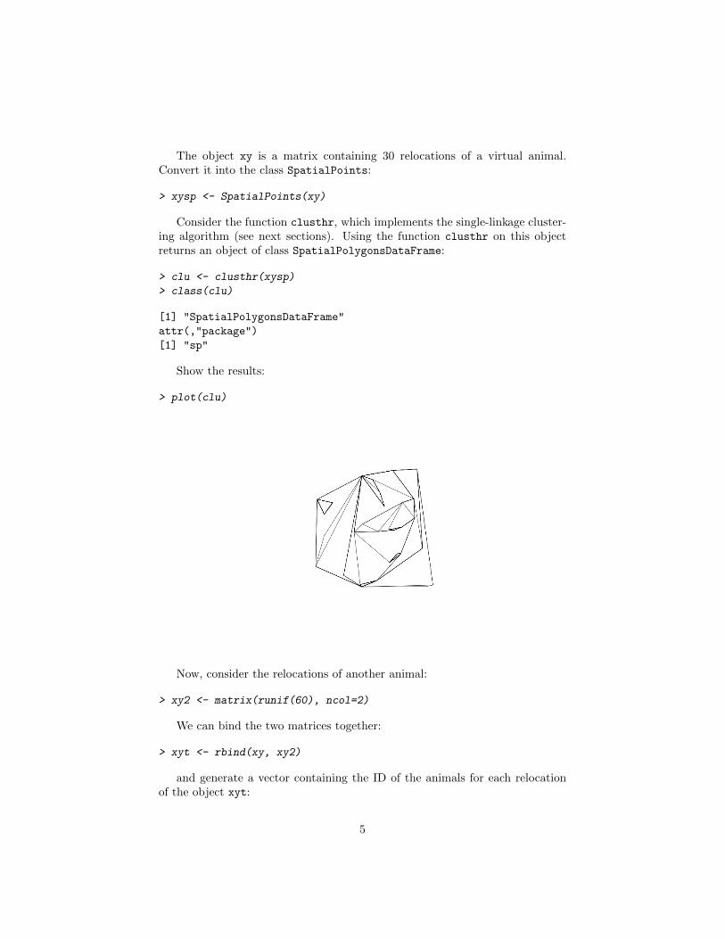
The object xy is a matrix containing 30 relocations of a virtual animal.Convert it into the class SpatialPoints:

> xysp <- SpatialPoints(xy)

Consider the function clusthr, which implements the single-linkage cluster-ing algorithm (see next sections). Using the function clusthr on this objectreturns an object of class SpatialPolygonsDataFrame:

> clu <- clusthr(xysp)

> class(clu)

[1] "SpatialPolygonsDataFrame"

attr(,"package")

[1] "sp"

Show the results:

> plot(clu)

Now, consider the relocations of another animal:

> xy2 <- matrix(runif(60), ncol=2)

We can bind the two matrices together:

> xyt <- rbind(xy, xy2)

and generate a vector containing the ID of the animals for each relocationof the object xyt:

5

> id <- gl(2,30)

We can convert the object id into a SpatialPointsDataFrame:

> idsp <- data.frame(id)

> coordinates(idsp) <- xyt

> class(idsp)

[1] "SpatialPointsDataFrame"

attr(,"package")

[1] "sp"

And we can use the same function clusthr on this new object:

> clu2 <- clusthr(idsp)

> class(clu2)

[1] "MCHu"

> clu2

********** Multiple convex hull Home range of several Animals ************

This object is a list with one component per animal.

Each component is an object of class SpatialPolygonsDataFrame

The home range has been estimated for the following animals:

[1] "1" "2"

An object of the class "MCHu" is basically a list of objects of class Spa-

tialPolygonsDataFrame, with one element per animal. Thus:

> length(clu2)

[1] 2

> class(clu2[[1]])


attr(,"package")

[1] "sp"

> class(clu2[[2]])


attr(,"package")

[1] "sp"

Although each SpatialPolygonsDataFrame of the list can be easily handledby the functions of the package sp and relatives (maptools, etc.), the packageadehabitatHR also contains functions allowing to deal with such lists. Forexample:

6

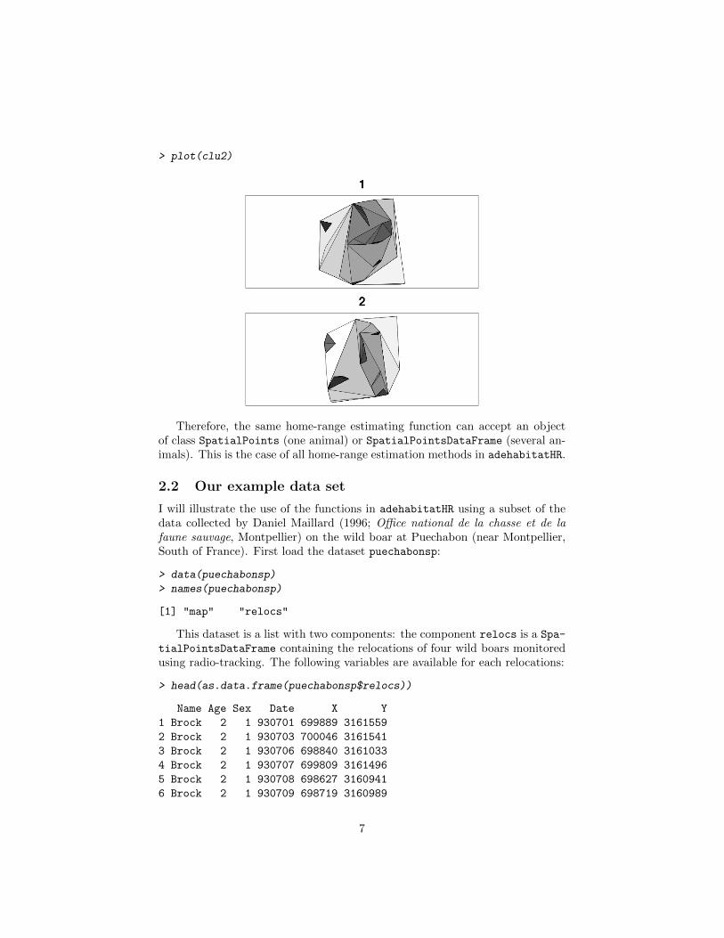
> plot(clu2)

Therefore, the same home-range estimating function can accept an objectof class SpatialPoints (one animal) or SpatialPointsDataFrame (several an-imals). This is the case of all home-range estimation methods in adehabitatHR.

2.2 Our example data set

I will illustrate the use of the functions in adehabitatHR using a subset of thedata collected by Daniel Maillard (1996; Office national de la chasse et de lafaune sauvage, Montpellier) on the wild boar at Puechabon (near Montpellier,South of France). First load the dataset puechabonsp:

> data(puechabonsp)

> names(puechabonsp)

[1] "map" "relocs"

This dataset is a list with two components: the component relocs is a Spa-

tialPointsDataFrame containing the relocations of four wild boars monitoredusing radio-tracking. The following variables are available for each relocations:

> head(as.data.frame(puechabonsp$relocs))

Name Age Sex Date X Y

1 Brock 2 1 930701 699889 3161559

2 Brock 2 1 930703 700046 3161541

3 Brock 2 1 930706 698840 3161033

4 Brock 2 1 930707 699809 3161496

5 Brock 2 1 930708 698627 3160941

6 Brock 2 1 930709 698719 3160989

7

The first variable is the identity of the animals, and we will use it in theestimation process.

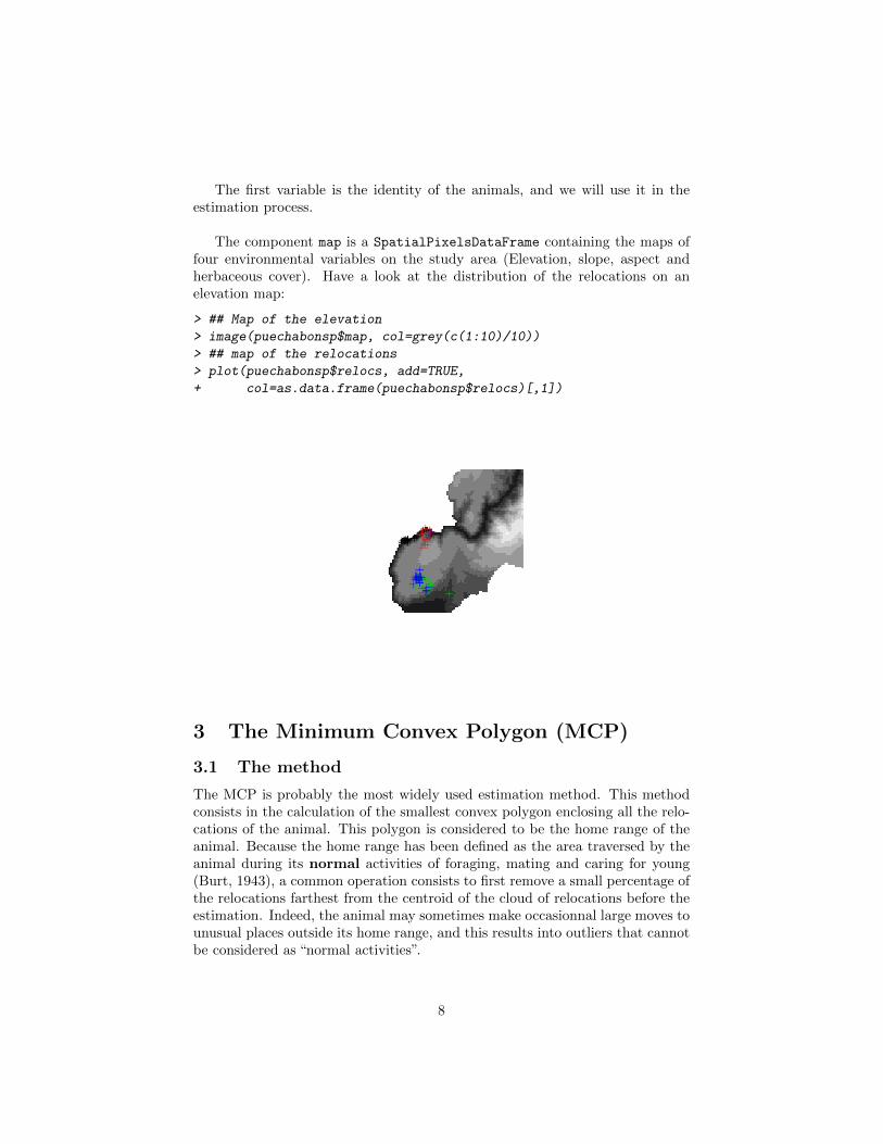
The component map is a SpatialPixelsDataFrame containing the maps offour environmental variables on the study area (Elevation, slope, aspect andherbaceous cover). Have a look at the distribution of the relocations on anelevation map:

> ## Map of the elevation

> image(puechabonsp$map, col=grey(c(1:10)/10))

> ## map of the relocations

> plot(puechabonsp$relocs, add=TRUE,

+ col=as.data.frame(puechabonsp$relocs)[,1])

3 The Minimum Convex Polygon (MCP)

3.1 The method

The MCP is probably the most widely used estimation method. This methodconsists in the calculation of the smallest convex polygon enclosing all the relo-cations of the animal. This polygon is considered to be the home range of theanimal. Because the home range has been defined as the area traversed by theanimal during its normal activities of foraging, mating and caring for young(Burt, 1943), a common operation consists to first remove a small percentage ofthe relocations farthest from the centroid of the cloud of relocations before theestimation. Indeed, the animal may sometimes make occasionnal large moves tounusual places outside its home range, and this results into outliers that cannotbe considered as “normal activities”.

8

3.2 The function mcp and interaction with the package sp

The function mcp allows the MCP estimation. For example, using the puech-

abonsp dataset, we estimate here the MCP of the monitored wild boars (afterthe removal of 5% of extreme points). Remember that the first column ofpuechabonsp$relocs is the identity of the animals:

> data(puechabonsp)

> cp <- mcp(puechabonsp$relocs[,1], percent=95)

The results are stored in an object of class SpatialPolygonsDataFrame:

> class(cp)


attr(,"package")

[1] "sp"

Therefore the functions available in the package sp and related packages(maptools, etc.) are available to deal with these objects. For example, thefunction plot:

> plot(cp)

> plot(puechabonsp$relocs, add=TRUE)

Similarly, the function writePolyShape from the package maptools can beused to export the object cp to a shapefile, so that it can be read into a GIS:

> library(maptools)

> writePolyShape(cp, "homerange")

The resulting shapefils can be read in any GIS.

9

3.3 Overlay operations

The function over of the package sp allows to combine points (including grid ofpixels) and polygons for points-in-polygon operations (see the help page of thisfunction). For example, the element map of the dataset puechabonsp is a mapof the study area according to four variables:

> head(as.data.frame(puechabonsp$map))

Elevation Aspect Slope Herbaceous x y

2017 68 3 1.548994 0 698800 3156800

2018 69 3 1.118594 0 698900 3156800

2019 70 3 1.358634 0 699000 3156800

2020 70 3 1.724311 0 699100 3156800

2021 70 3 1.944885 0 699200 3156800

2022 71 3 2.024868 0 699300 3156800

This object is of the class SpatialPixelsDataFrame. We may identify thepixels of this map enclosed in each home range using the function over fromthe package sp. For example, to identify the pixels enclosed in the home rangeof the second animal:

> enc <- over(puechabonsp$map, cp[,2], fn=function(x) return(1))

> head(enc)

area

1 NA

2 NA

3 NA

4 NA

5 NA

6 NA

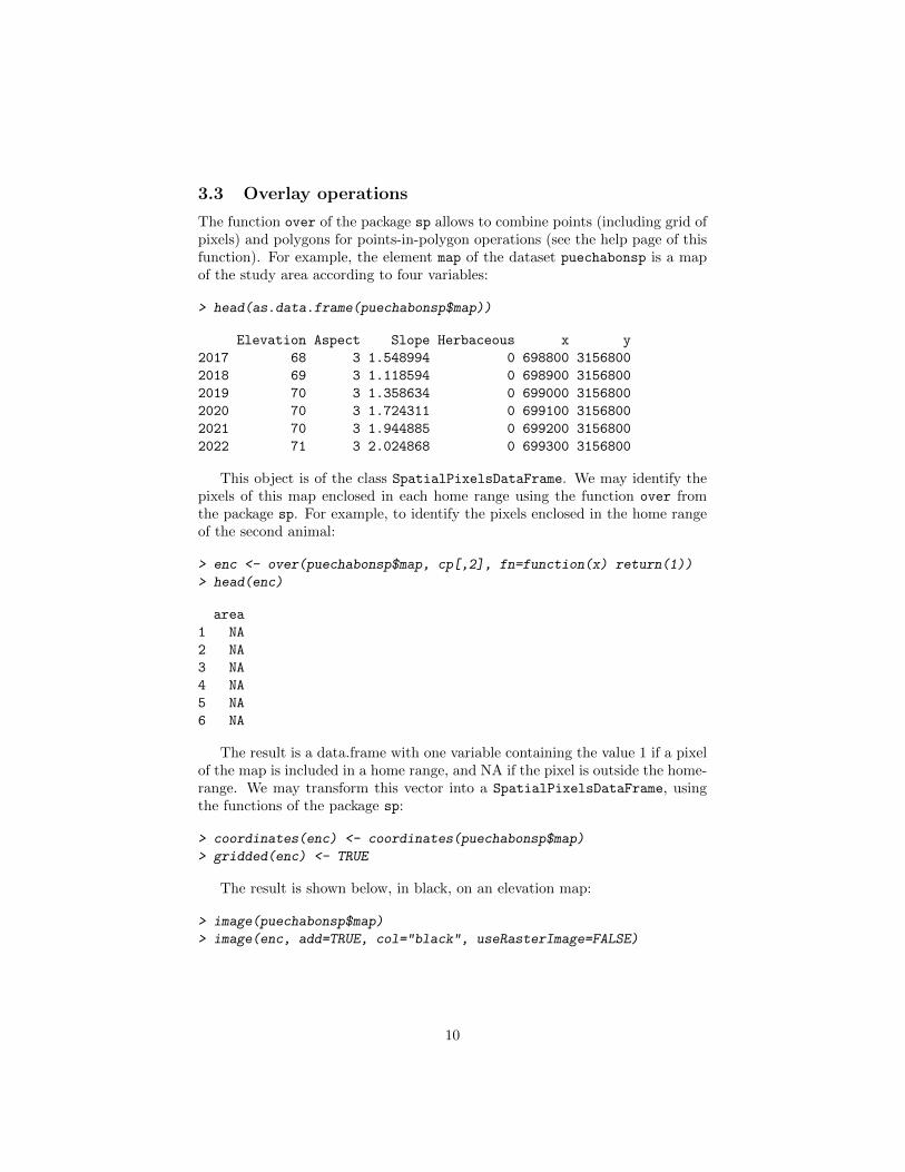
The result is a data.frame with one variable containing the value 1 if a pixelof the map is included in a home range, and NA if the pixel is outside the home-range. We may transform this vector into a SpatialPixelsDataFrame, usingthe functions of the package sp:

> coordinates(enc) <- coordinates(puechabonsp$map)

> gridded(enc) <- TRUE

The result is shown below, in black, on an elevation map:

> image(puechabonsp$map)

> image(enc, add=TRUE, col="black", useRasterImage=FALSE)

10

However, because the rasterization of home ranges is a common operation,I included a function hr.rast to make this operation more straightforward:

> cprast <- hr.rast(cp, puechabonsp$map)

The resulting object is a SpatialPixelsDataFrame with one column peranimal:

> par(mar=c(0,0,0,0))

> par(mfrow=c(2,2))

> for (i in 1:4) {

+ image(cprast[,i], useRasterImage=FALSE)

+ box()

+ }

11

3.4 Computation of the home-range size

The home range size is automatically computed by the function mcp. Thus,coercing the object returned by the function to the class data.frame givesaccess to the home range size:

> as.data.frame(cp)

id area

Brock Brock 22.64670

Calou Calou 41.68815

Chou Chou 71.93205

Jean Jean 55.88415

The area is here expressed in hectares (the original units in the object puech-abonsp$relocs were expressed in metres). The units of the results and of theoriginal data are controlled by the arguments unin and unout of the functionmcp (see the help page of the function mcp). We did not change the units in ourexample estimation, as the default was a suitable choice.

In this example, we have chosen to exclude 5% of the mst extreme relocations,but we could have made another choice. We may compute the home-range sizefor various choices of the number of extreme relocations to be excluded, usingthe function mcp.area:

> hrs <- mcp.area(puechabonsp$relocs[,1], percent=seq(50, 100, by = 5))

12

Here, except for Calou, the choice to exclude 5% of the relocations seems asensible one. In the case of Calou, it is disputable to remove 20% of the relo-cations to achieve an asymptote in the home range size decrease. 20% of thetime spent in an area is no longer an exceptionnal activity... and this area couldbe considered as part of the home range. Under these conditions, the choice tocompute the MCP with 95% of the relocations for all animals seems a sensibleone.

Note that the results of the function mcp.area are stored in a data frame ofclass "hrsize" and can be used for further analysis:

> hrs

Brock Calou Chou Jean

50 9.68735 16.31155 26.76340 5.72115

55 9.85540 16.31155 28.51200 5.99155

60 12.84635 17.49680 29.97835 6.64385

65 13.12805 19.74600 31.75860 9.05275

70 15.66545 20.05745 32.25850 10.58390

75 16.14625 21.53025 34.77430 16.40945

80 19.06725 22.15015 47.81925 24.29185

85 20.22535 26.75180 54.76550 35.31225

90 21.82440 37.12975 67.18565 52.59315

95 22.64670 41.68815 71.93205 55.88415

100 40.59635 49.75050 162.84550 167.63690

This class of data is common in adehabitatHR and we will generate againsuch objects with other home range estimation methods.

13

4 The kernel estimation and the utilization dis-tribution

4.1 The utilization distribution

The MCP has met a large success in the ecological literature. However, manyauthors have stressed that the definition of the home range which is commonlyused in the literature was rather imprecise: “that area traversed by the animalduring its normal activities of food gathering, mating and caring for young”(Burt, 1943). Although this definition corresponds well to the feeling of manyecologists concerning what is the home range, it lacks formalism: what is anarea traversed? what is a normal activity?

Several authors have therefore proposed to replace this definition by a moreformal model: the utilization distribution (UD, van Winkle, 1975). Under thismodel, we consider that the animals use of space can be described by a bivariateprobability density function, the UD, which gives the probability density torelocate the animal at any place according to the coordinates (x, y) of thisplace. The study of the space use by an animal could consist in the study ofthe properties of the utilization distribution. The issue is therefore to estimatethe utilization distribution from the relocation data:

The seminal paper of Worton (1989) proposed the use of the kernel method(Silverman, 1986; Wand and Jones, 1995) to estimate the UD using the re-location data. The kernel method was probably the most frequently usedfunction in the package adehabitat. A lot of useful material and informa-tion on its use can be found on the website of the group Animove (http://www.faunalia.it/animov/). I give here a summary of the discussion found

14

http://www.faunalia.it/animov/


on this site (they include answers to the most frequently asked questions).

The basic principle of the method is the following: a bivariate kernel functionis placed over each relocation, and the values of these functions are averagedtogether.

Many kernel functions K can be used in the estimation process providedthat: ∫

K(x) = 1

and

K(x) > 0 ∀x

where x is a vector containing the coordinates of a point on the plane.However, there are two common choices for the kernel functions: the bivariatenormal kernel:

K(x) =1

2πexp(−1

2xtx)

and the Epanechnikov kernel:

K(x) =3

4(1− xtx) if x < 1 or 0 otherwise

The choice of a kernel function does not greatly affect the estimates (Sil-verman, 1986; Wand and Jones, 1995). Although the Epanechnikov kernel isslightly more efficient, the bivariate normal kernel is still a common choice (andis the default choice in adehabitatHR).

Then, the kernel estimation of the UD at a given point x of the plane isobtained by:

f̂(x) =1

nh2

n∑i=1

K

{1

h(x−Xi)

}where h is a smoothing parameter, n is the number of relocations, and Xi

is the ith relocation of the sample.

The smoothing parameter h controls the “width” of the kernel functionsplaced over each point. On an example dataset:

15

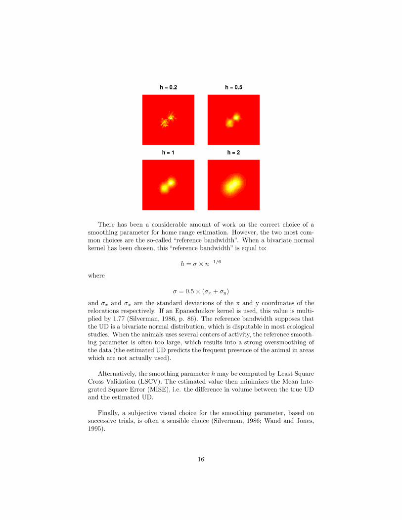
There has been a considerable amount of work on the correct choice of asmoothing parameter for home range estimation. However, the two most com-mon choices are the so-called “reference bandwidth”. When a bivariate normalkernel has been chosen, this “reference bandwidth” is equal to:

h = σ × n−1/6

where

σ = 0.5× (σx + σy)

and σx and σx are the standard deviations of the x and y coordinates of therelocations respectively. If an Epanechnikov kernel is used, this value is multi-plied by 1.77 (Silverman, 1986, p. 86). The reference bandwidth supposes thatthe UD is a bivariate normal distribution, which is disputable in most ecologicalstudies. When the animals uses several centers of activity, the reference smooth-ing parameter is often too large, which results into a strong oversmoothing ofthe data (the estimated UD predicts the frequent presence of the animal in areaswhich are not actually used).

Alternatively, the smoothing parameter h may be computed by Least SquareCross Validation (LSCV). The estimated value then minimizes the Mean Inte-grated Square Error (MISE), i.e. the difference in volume between the true UDand the estimated UD.

Finally, a subjective visual choice for the smoothing parameter, based onsuccessive trials, is often a sensible choice (Silverman, 1986; Wand and Jones,1995).

16

4.2 The function kernelUD: estimating the utilization dis-tribution

The function kernelUD of the package adehabitatHR implements the methoddescribed above to estimate the UD. The UD is estimated in each pixel of agrid superposed to the relocations. I describe in the next sections how the gridparameters can be controlled in the estimation. Similarly to all the functionsallowing the estimation of the home range, the functions may take as argumenteither a SpatialPoints object (estimation of the UD of one animal) or a Spa-

tialPointsDataFrame object with one column corresponding to the identity ofthe animal (estimation of the UD of several animals). The argument h controlsthe value of the smoothing parameter. Thus, if h = "href", the “reference”bandwidth is used in the estimation. If h = "LSCV", the “LSCV” bandwidth isused in the estimation. Alternatively, it is possible to pass a numeric value forthe smoothing parameter.

I give below a short example of the use of kernelUD, using the puechabonsp

dataset. Remember that the first column of the component relocs of thisdataset contains the identity of the animals:

> data(puechabonsp)

> kud <- kernelUD(puechabonsp$relocs[,1], h="href")

> kud

********** Utilization distribution of several Animals ************

Type: probability density

Smoothing parameter estimated with a href smoothing parameter


Each component is an object of class estUD

See estUD-class for more information

The resulting object is a list of the class "estUD". This class extends theclass SpatialPixelsDataFrame (it just contains an additional attribute storingthe information about the smoothing parameter). Display the results:

> image(kud)

17

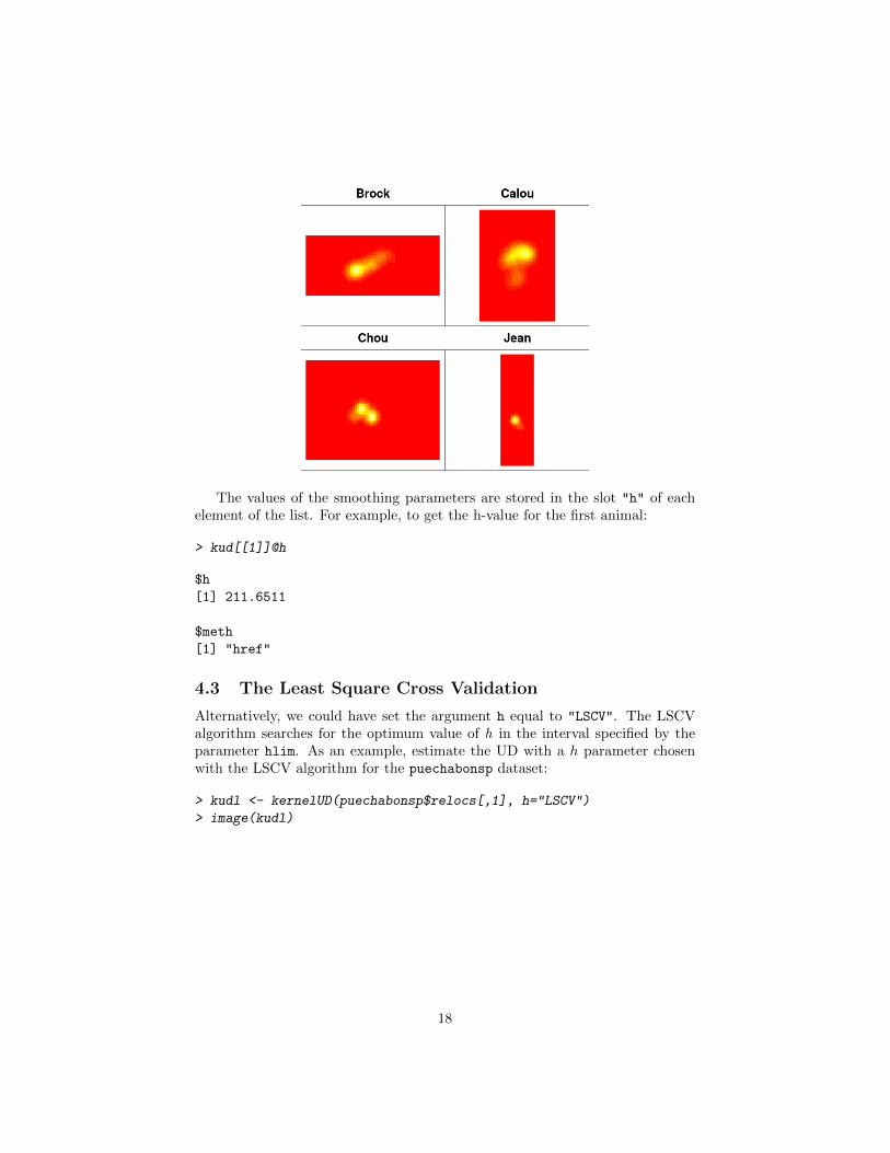
The values of the smoothing parameters are stored in the slot "h" of eachelement of the list. For example, to get the h-value for the first animal:

> kud[[1]]@h

$h

[1] 211.6511

$meth

[1] "href"

4.3 The Least Square Cross Validation

Alternatively, we could have set the argument h equal to "LSCV". The LSCValgorithm searches for the optimum value of h in the interval specified by theparameter hlim. As an example, estimate the UD with a h parameter chosenwith the LSCV algorithm for the puechabonsp dataset:

> kudl <- kernelUD(puechabonsp$relocs[,1], h="LSCV")

> image(kudl)

18

The resulting UD fits the data more closely than the use of “href”. However,note that the cross-validation criterion cannot be minimized in some cases. Ac-cording to Seaman and Powell (1998) ”This is a difficult problem that has notbeen worked out by statistical theoreticians, so no definitive response is avail-able at this time”. Therefore, it is essential to look at the results of the LSCVminimization using the function plotLSCV:

> plotLSCV(kudl)

19

Here, the minimization has been achieved in the specified interval. Whenthe algorithm does not converge toward a solution, the estimate should notbe used in further analysis. Solutions are discussed on the animove website(http://www.faunalia.it/animov/), and especially on the mailing list. Inparticular, see the following messages:

• http://www.faunalia.com/pipermail/animov/2006-May/000137.html



Finally, the user may indicate a numeric value for the smoothing param-eter. Further discussion on the choice of h-values can be found on the ani-move website, at the URL: https://www.faunalia.it/dokuwiki/doku.php?id=public:animove.

4.4 Controlling the grid

The UD is estimated at the center of each pixel of a grid. Although the sizeand resolution of the grid does not have a large effect on the estimates (seeSilverman, 1986), it is sometimes useful to be able to control the parametersdefining this grid. This is done thanks to the parameter grid of the functionkernelUD.

4.4.1 Passing a numeric value

When a numeric value is passed to the parameter grid, the function kernelUD

automatically computes the grid for the estimation. This grid is computed inthe following way:

• the minimum and maximum coordinates (Xmin, Xmax, Ymin, Ymax) of therelocations are computed.

• the range of X and Y values is also computed (i.e., the difference betweenthe maximum and minimum value). Let Rx and RY be these ranges.

• The coverage of the grid is defined thanks to the parameter extent of thefunction kernelUD. Let e be this parameter. The minimum and maxi-mum X coordinates of the pixels of the grid are equal to Xmin − e × Rx

and Xmax + e × Rx respectively. Similarly, the minimum and maximumY coordinates of the pixels of the grid are equal to Ymin − e × RY andYmax + e×RY respectively.

20


http://www.faunalia.com/pipermail/animov/2006-May/000137.html



https://www.faunalia.it/dokuwiki/doku.php?id=public:animove

https://www.faunalia.it/dokuwiki/doku.php?id=public:animove

• Finally, these extents are split into g intervals, where g is the value of theparameter grid.

Consequently, the parameter grid controls the resolution of the grid and theparameter extent controls its extent. As an illustration, consider the estimateof the first animal:

> ## The relocations of "Brock"

> locs <- puechabonsp$relocs

> firs <- locs[as.data.frame(locs)[,1]=="Brock",]

> ## Graphical parameters

> par(mar=c(0,0,2,0))

> par(mfrow=c(2,2))

> ## Estimation of the UD with grid=20 and extent=0.2

> image(kernelUD(firs, grid=20, extent=0.2))

> title(main="grid=20, extent=0.2")


> image(kernelUD(firs, grid=80, extent=0.2))

> title(main="grid=80, extent=0.2")


> image(kernelUD(firs, grid=20, extent=3))

> title(main="grid=20, extent=3")


> image(kernelUD(firs, grid=80, extent=3))

> title(main="grid=80, extent=3")

Note that the parameter same4all is an additional parameter allowing thecontrol of the grid. If it is equal to TRUE, the same grid is used for all animals,thus for example:

21

> kus <- kernelUD(puechabonsp$relocs[,1], same4all=TRUE)

> image(kus)

Because all the UD are estimated on the same grid, it is possible to coercethe resulting object as a SpatialPixelsDataFrame:

> ii <- estUDm2spixdf(kus)

> class(ii)

[1] "SpatialPixelsDataFrame"

attr(,"package")

[1] "sp"

This object can then be handed with the functions of the package sp.

4.4.2 Passing a SpatialPixelsDataFrame

It is sometimes useful to estimate the UD in each pixel of a raster map alreadyavailable. This can be useful in habitat selection studies, when the value of theUD is to be later related to the value of environmental variables. In such cases,it is possible to pass a raster map to the parameter grid of the function. Forexample, the dataset puechabonsp contains an object of class SpatialPixels-DataFrame storing the environmental information for this variable. This mapcan be passed to the parameter grid:

> kudm <- kernelUD(puechabonsp$relocs[,1], grid=puechabonsp$map)

And as in the previous section, the object can be coerced into a SpatialPix-

elsDataFrame using the function estUDm2spixdf. Note also that it is possibleto pass a list of SpatialPixelsDataFrame (with one element per animal) to theparameter grid (see the help page of the function kernelUD).

22

4.5 Estimating the home range from the UD

The UD gives the probability density to relocate the animal at a given place. Thehome range deduced from the UD as the minimum area on which the probabilityto relocate the animal is equal to a specified value. For example, the 95% homerange corresponds to the smallest area on which the probability to relocate theanimal is equal to 0.95. The functions getvolumeUD and getverticeshr provideutilities for home range estimation.

4.5.1 Home ranges in vector mode

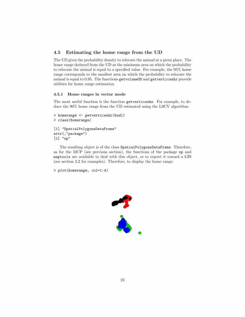
The most useful function is the function getverticeshr. For example, to de-duce the 90% home range from the UD estimated using the LSCV algorithm:

> homerange <- getverticeshr(kudl)

> class(homerange)


attr(,"package")

[1] "sp"

The resulting object is of the class SpatialPolygonsDataFrame. Therefore,as for the MCP (see previous section), the functions of the package sp andmaptools are available to deal with this object, or to export it toward a GIS(see section 3.2 for examples). Therefore, to display the home range:

> plot(homerange, col=1:4)

23

4.5.2 Home ranges in raster mode

However, the function getverticeshr returns an object of class SpatialPoly-gonsDataFrame, i.e. an object in mode vector.

The function getvolumeUD may also be useful to estimate the home range inraster mode, from the UD. Actually, this function modifies the UD componentof the object passed as argument, so that the value of a pixel is equal to thepercentage of the smallest home range containing this pixel:

> vud <- getvolumeUD(kudl)

> vud

********** Utilization distribution of several Animals ************

Type: volume under UD

Smoothing parameter estimated with a LSCV smoothing parameter


Each component is an object of class estUD


To make clear the differences between the output of kernelUD and getvol-

umeUD look at the values on the following contourplot:

> ## Set up graphical parameters

> par(mfrow=c(2,1))

> par(mar=c(0,0,2,0))

> ## The output of kernelUD for the first animal

> image(kudl[[1]])

> title("Output of kernelUD")

> ## Convert into a suitable data structure for

> ## the use of contour

> xyz <- as.image.SpatialGridDataFrame(kudl[[1]])

> contour(xyz, add=TRUE)

> ## and similarly for the output of getvolumeUD

> par(mar=c(0,0,2,0))

> image(vud[[1]])

> title("Output of getvolumeUD")

> xyzv <- as.image.SpatialGridDataFrame(vud[[1]])

> contour(xyzv, add=TRUE)

24

Whereas the output of kernelUD is the raw UD, the output of getvol-

umeUD can be used to compute the home range (the labels of the contour linescorrespond to the home ranges computed with various probability levels). Forexample, to get the rasterized 95% home range of the first animal:

> ## store the volume under the UD (as computed by getvolumeUD)

> ## of the first animal in fud

> fud <- vud[[1]]

> ## store the value of the volume under UD in a vector hr95

> hr95 <- as.data.frame(fud)[,1]

> ## if hr95 is <= 95 then the pixel belongs to the home range

> ## (takes the value 1, 0 otherwise)

25

> hr95 <- as.numeric(hr95 <= 95)

> ## Converts into a data frame

> hr95 <- data.frame(hr95)

> ## Converts to a SpatialPixelsDataFrame

> coordinates(hr95) <- coordinates(vud[[1]])

> gridded(hr95) <- TRUE

> ## display the results

> image(hr95)

4.6 The home range size

As for the MCP, the SpatialPolygonsDataFrame returned by the functiongetverticeshr contains a column named “area”, which contains the area ofthe home ranges:

> as.data.frame(homerange)

id area

Brock Brock 71.98975

Calou Calou 82.39555

Chou Chou 135.51111

Jean Jean 109.82873

And, as for the MCP, the units of these areas are controlled by the parametersunin and unout of the function getverticeshr.

I also considered that it would be useful to have a function which wouldcompute the home-range size for several probability levels. This is the aim ofthe function kernel.area which takes the UD as argument (here we use theUD estimated with the LSCV algorithm).

26

> ii <- kernel.area(kudl, percent=seq(50, 95, by=5))

> ii

Brock Calou Chou Jean

50 15.23389 19.63337 28.19983 15.27989

55 18.44102 22.90559 33.57122 18.33587

60 21.64816 26.83227 38.94262 24.44782

65 24.85529 31.41339 45.65686 27.50380

70 28.06243 36.32173 53.71395 36.67174

75 32.87313 41.88452 61.77105 42.78369

80 37.68383 48.10175 73.85669 51.95163

85 44.89988 55.62787 87.28518 61.11956

90 52.91772 65.77178 103.39936 73.34347

95 67.34983 80.16958 130.25634 100.84728

The resulting object is of the class hrsize, and can be plotted using the func-tion plot. Note that the home-range sizes returned by this function are slightlydifferent from the home-range size stored in the SpatialPolygonsDataFrame

returned by the function getverticeshr. Indeed, while the former measuresthe area covered by the rasterized home range (area covered by the set of pixelsof the grid included in the home range), the latter measures the area of thevector home range (with smoother contour). However, note that the differencebetween the two estimates decrease as the resolution of the grid becomes finer.

4.7 Taking into account the presence of physical boundaryover the study area

In a recent paper, Benhamou and Cornelis (2010) proposed an interesting ap-proach to take into account the presence of physical boundaries on the studyarea. They proposed to extend to 2 dimensions a method developed for one di-mension by Silverman 1986. The principle of this approach is described below:

27

On this figure, the relocations are located near the lower left corner of themap. The line describes a physical boundary located on the study area (e.g. acliff, a pond, etc.). The animal cannot cross the boundary. The use of the clas-sical kernel estimation will not take into account this boundary when estimatingthe UD. A classical approach when such problem occur is to use the classicalkernel approach and then to set to 0 the value of the UD on the other side ofthe boundary. However, this may lead to some bias in the estimation of theUD near the boundary (as the kernel estimation will “smooth” the use acrossthe boundary, whereas one side of the boundary is used and the other unused).Benhamou and Cornelis (2010) extended an approach developed for kernel esti-mation in one dimension: this approach consists in calculating the mirror imageof the points located near the boundary, and adding these “mirror points” to theactual relocations before the kernel estimation (These mirror points correspondto the crosses on the figure). Note that this approach cannot be used forall boundaries. There are two constraints that have to be satisfied:

• The boundary should be defined as the union of several segments, and eachsegment length should at least be equal to 3× h, where h is the smoothingparameter used for kernel smoothing;

• The angle between two successive line segments should be greater thatπ/2 or lower than −π/2.

Therefore, the boundary shape should be fairly simple, and not too tortuous.

Now, let us consider the case of the wild boar monitored in Puechabon.Consider the map of the elevation on the study area:

28


This area is traversed by the Herault gorges. As can be seen on this figure,the slopes of the gorges are very steep, and it is nearly impossible for the wildboars monitored to cross the river (although it is possible in other places).Therefore, the gorges are a boundary that cannot be crossed by the animal.Using the function locator(), we have defined the following boundary:

> bound <- structure(list(x = c(701751.385381925, 701019.24105475,

+ 700739.303517889,

+ 700071.760160759, 699522.651915378,

+ 698887.40904327, 698510.570051342,

+ 698262.932999504, 697843.026694212,

+ 698058.363261028),

+ y = c(3161824.03387414,

+ 3161824.03387414, 3161446.96718494,

+ 3161770.16720425, 3161479.28718687,

+ 3161231.50050539, 3161037.5804938,

+ 3160294.22044937, 3159389.26039528,

+ 3157482.3802813)), .Names = c("x", "y"))


> lines(bound, lwd=3)

29

We now convert this boundary as a SpatialLines object:

> ## We convert bound to SpatialLines:

> bound <- do.call("cbind",bound)

> Slo1 <- Line(bound)

> Sli1 <- Lines(list(Slo1), ID="frontier1")

> barrier <- SpatialLines(list(Sli1))

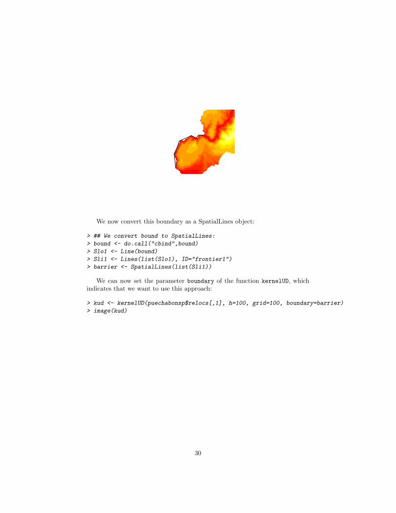
We can now set the parameter boundary of the function kernelUD, whichindicates that we want to use this approach:

> kud <- kernelUD(puechabonsp$relocs[,1], h=100, grid=100, boundary=barrier)

> image(kud)

30

The effect of the boundary correction is clear on the UD of Brock and Calou.

5 Taking into account the time dependence be-tween relocation

5.1 The Brownian bridge kernel method

5.1.1 Description

Bullard (1999) proposed an extension of the kernel method taking into accountthe time dependence between successive relocations. Whereas the classical ker-

31

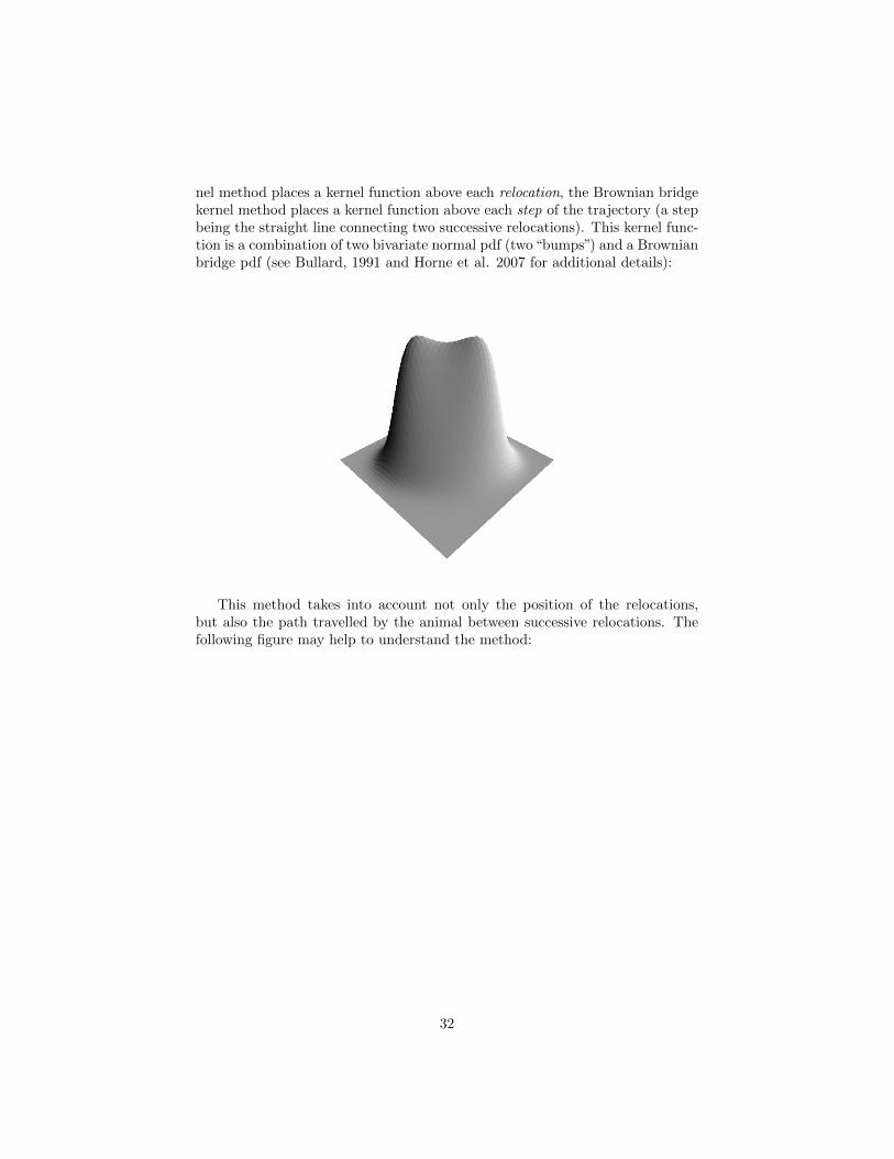
nel method places a kernel function above each relocation, the Brownian bridgekernel method places a kernel function above each step of the trajectory (a stepbeing the straight line connecting two successive relocations). This kernel func-tion is a combination of two bivariate normal pdf (two“bumps”) and a Brownianbridge pdf (see Bullard, 1991 and Horne et al. 2007 for additional details):

This method takes into account not only the position of the relocations,but also the path travelled by the animal between successive relocations. Thefollowing figure may help to understand the method:

32

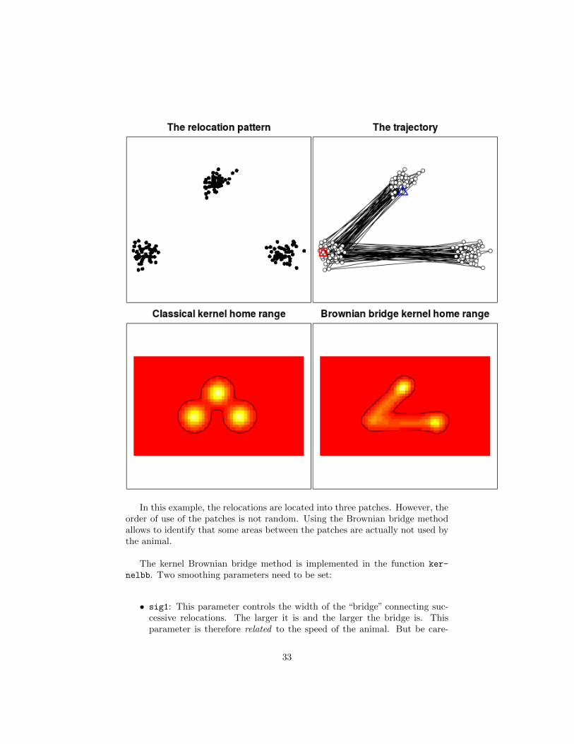
In this example, the relocations are located into three patches. However, theorder of use of the patches is not random. Using the Brownian bridge methodallows to identify that some areas between the patches are actually not used bythe animal.

The kernel Brownian bridge method is implemented in the function ker-

nelbb. Two smoothing parameters need to be set:

• sig1: This parameter controls the width of the “bridge” connecting suc-cessive relocations. The larger it is and the larger the bridge is. Thisparameter is therefore related to the speed of the animal. But be care-

33

ful: it is not the speed of the animal. Horne et al. (2007) call sig12 the“Brownian motion variance parameter”. It is even not the variance of theposition, but a parameter used to compute the variance (which is itselfrelated to the speed). The variance of the position of the animal betweentwo relocations at time t is S2 = sig12 × t × (T − t)/T , where T is theduration of the trajectory between the two relocations and t the time atthe current position. Therefore, sig1 is related to the speed of the ani-mal in a very complex way, and its biological meaning is not that clear.The definition of sig1 can be done subjectively after visual explorationof the result for different values, or using the function liker that imple-ments the maximum likelihood approach developed by Horne et al. (2007);

• sig2: This parameter controls the width of the “bumps” added over therelocations (see Bullard, 1999; Horne et al. 2007). It is similar to thesmoothing parameter h of the classical kernel method, and is thereforerelated to the imprecision of the relocations.

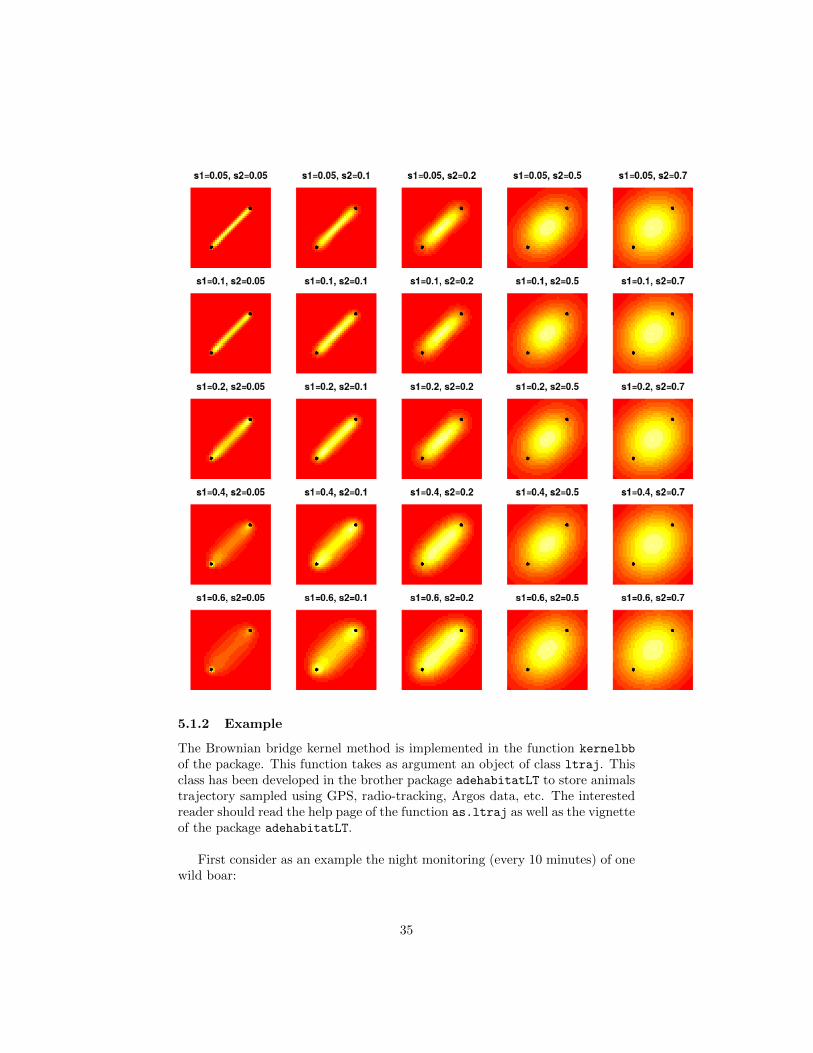
The following figure shows the kernel function placed over the step built bythe two relocations (0,0) and (1,1), for different values of sig1 and sig2:

34

5.1.2 Example

The Brownian bridge kernel method is implemented in the function kernelbb

of the package. This function takes as argument an object of class ltraj. Thisclass has been developed in the brother package adehabitatLT to store animalstrajectory sampled using GPS, radio-tracking, Argos data, etc. The interestedreader should read the help page of the function as.ltraj as well as the vignetteof the package adehabitatLT.

First consider as an example the night monitoring (every 10 minutes) of onewild boar:

35

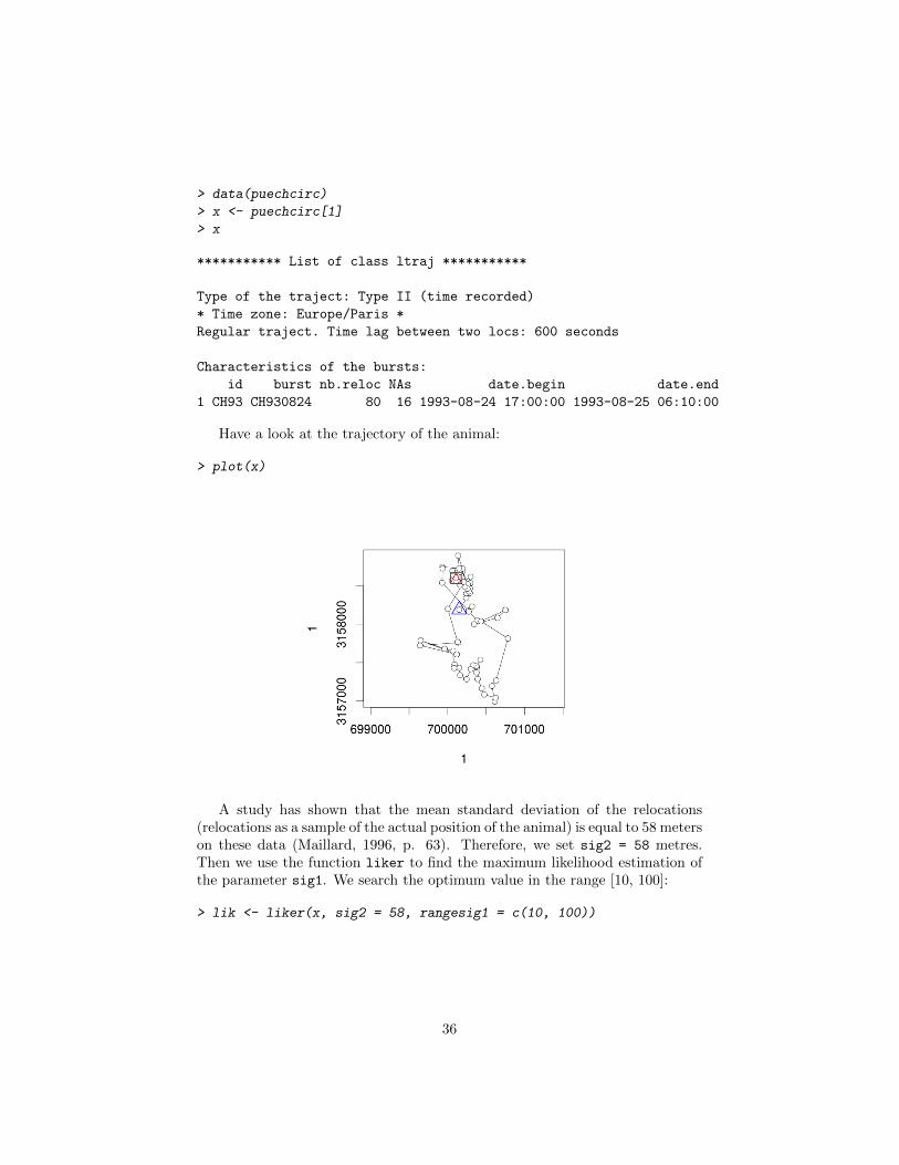
> data(puechcirc)

> x <- puechcirc[1]

> x

*********** List of class ltraj ***********

Type of the traject: Type II (time recorded)

* Time zone: Europe/Paris *

Regular traject. Time lag between two locs: 600 seconds

Characteristics of the bursts:

id burst nb.reloc NAs date.begin date.end

1 CH93 CH930824 80 16 1993-08-24 17:00:00 1993-08-25 06:10:00

Have a look at the trajectory of the animal:

> plot(x)

A study has shown that the mean standard deviation of the relocations(relocations as a sample of the actual position of the animal) is equal to 58 meterson these data (Maillard, 1996, p. 63). Therefore, we set sig2 = 58 metres.Then we use the function liker to find the maximum likelihood estimation ofthe parameter sig1. We search the optimum value in the range [10, 100]:

> lik <- liker(x, sig2 = 58, rangesig1 = c(10, 100))

36

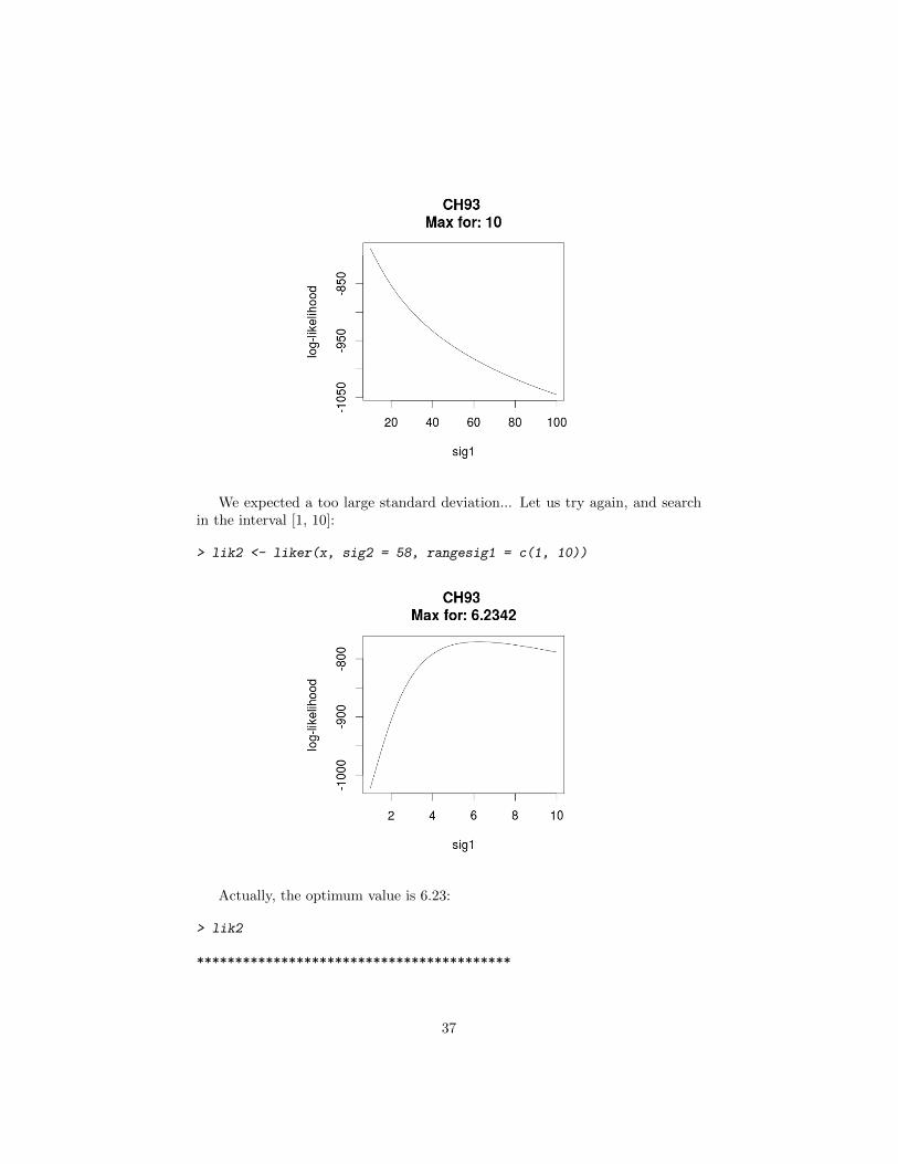
We expected a too large standard deviation... Let us try again, and searchin the interval [1, 10]:

> lik2 <- liker(x, sig2 = 58, rangesig1 = c(1, 10))

Actually, the optimum value is 6.23:

> lik2

*****************************************

37

Maximization of the log-likelihood for parameter

sig1 of brownian bridge

CH93 : Sig1 = 6.2342 Sig2 = 58

We can now estimate the kernel Brownian bridge home range with the pa-rameters sig1=6.23 and sig2=58:

> tata <- kernelbb(x, sig1 = 6.23, sig2 = 58, grid = 50)

> tata

********** Utilization distribution of an Animal ************


Smoothing parameter estimated with a BB-specified parameter

This object inherits from the class SpatialPixelsDataFrame.


The result is an object of class estUD, and can be managed as such (seesection 4.2). For example to see the utilization distribution and the 95% homerange:

> image(tata)

> plot(getverticeshr(tata, 95), add=TRUE, lwd=2)

5.2 The biased random bridge kernel method

5.2.1 Description

Benhamou and Cornelis (2010) developed an approach similar to the Brownianbridge method for the analysis of trajectories. They called it “movement based

38

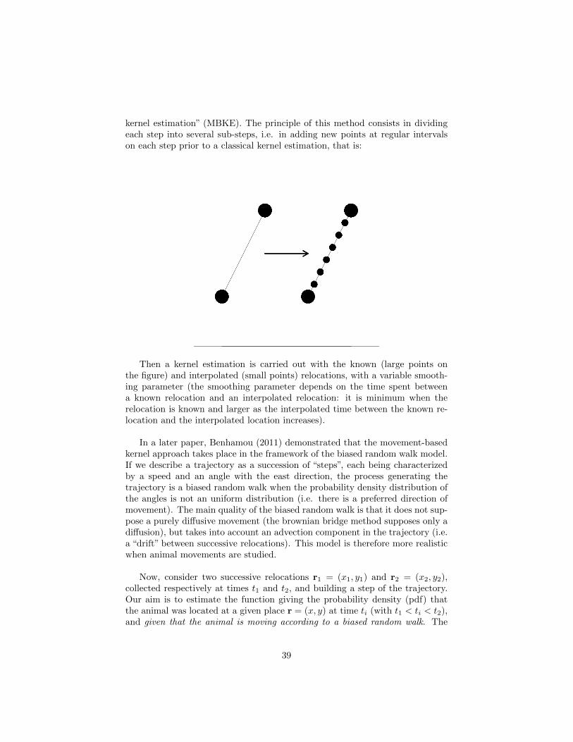
kernel estimation” (MBKE). The principle of this method consists in dividingeach step into several sub-steps, i.e. in adding new points at regular intervalson each step prior to a classical kernel estimation, that is:

Then a kernel estimation is carried out with the known (large points onthe figure) and interpolated (small points) relocations, with a variable smooth-ing parameter (the smoothing parameter depends on the time spent betweena known relocation and an interpolated relocation: it is minimum when therelocation is known and larger as the interpolated time between the known re-location and the interpolated location increases).

In a later paper, Benhamou (2011) demonstrated that the movement-basedkernel approach takes place in the framework of the biased random walk model.If we describe a trajectory as a succession of “steps”, each being characterizedby a speed and an angle with the east direction, the process generating thetrajectory is a biased random walk when the probability density distribution ofthe angles is not an uniform distribution (i.e. there is a preferred direction ofmovement). The main quality of the biased random walk is that it does not sup-pose a purely diffusive movement (the brownian bridge method supposes only adiffusion), but takes into account an advection component in the trajectory (i.e.a “drift” between successive relocations). This model is therefore more realisticwhen animal movements are studied.

Now, consider two successive relocations r1 = (x1, y1) and r2 = (x2, y2),collected respectively at times t1 and t2, and building a step of the trajectory.Our aim is to estimate the function giving the probability density (pdf) thatthe animal was located at a given place r = (x, y) at time ti (with t1 < ti < t2),and given that the animal is moving according to a biased random walk. The

39

movement generated by a biased random walk given the start and end relocationis called a biased random bridge (BRB). Benhamou (2011) noted that the BRBcan be approximated by a bivariate normal distribution:

f(r, ti|r1, r2) =t2 − t1

4πD(t2 − ti)exp

[rmDrm

4pi(t2 − ti)

](1)

where the mean location corresponds to rm = (x1+pi(x2−x1), y1+pi(y2−y1)),and pi = (ti − t1)/(t2 − t1). The variance-covariance matrix D of this distribu-tion usually cannot be estimated in practice (Benhamou, 2011). Consequently,the biased random bridge is approximated by a random walk with a diffusioncoefficient D on which a drift v is appended. And, under this assumption, therequired pdf can be approximated by a circular normal distribution fully inde-pendent of the drift, i.e. the matrix D in equation 1 is supposed diagonal, withboth diagonal elements corresponding to a diffusion coefficient D. The figurebelow illustrates how the pdf of relocating the animal changes with the timesti:

We can see that the variance of this distribution is larger when the animalis far from the known relocations.

Benhamou (2011) demonstrated that the MBKE can be used to estimate theUD of the animal under the hypothesis that the animal moves according to a bi-ased random walk, with a drift allowed to change in strength and direction fromone step to the next. However, it is supposed that the drift is constant duringeach step. For this reason, it is required to set an upper time threshold Tmax.Steps characterized by a longer duration are not taken into account into the es-timation of the UD. This upper threshold should be based on biological grounds.

40

As for the Brownian bridge approach, this conditional pdf based on BRBtakes an infinite value at times ti = t1 and ti = t2 (because, at these times,the relocation of the animal is known exactly). Benhamou (2011) proposed tocircumvent this drawback by considering that the true relocation of the animalat times t1 and t2 is not known exactly. He noted: “a GPS fix should be con-sidered a punctual sample of the possible locations at which the animal may beobserved at that time, given its current motivational state and history. Evenif the recording noise is low, the relocation variance should therefore be largeenough to encompass potential locations occurring in the same habitat patch asthe recorded location”. He proposed two ways to include this “relocation uncer-tainty” component in the pdf: (i) either the relocation variance progressivelymerges with the movement component, (ii) or the relocation variance has a con-stant weight.

In both cases, the minimum uncertainty over the relocation of an animal isobserved for ti = t1 or t2. This minimum standard deviation corresponds to theparameter hmin. According to Benhamou and Cornelis (2010), “hmin must beat least equal to the standard deviation of the localization errors and also mustintegrate uncertainty of the habitat map when UDs are computed for habitatpreference analyses. Beyond these technical constraints, hmin also should incor-porate a random component inherent to animal behavior because any recordedlocation, even if accurately recorded and plotted on a reliable map, is just a punc-tual sample of possible locations at which the animal may be found at that time,given its current motivational state and history. Consequently, hmin should belarge enough to encompass potential locations occurring in the same habitat patchas the recorded location”.

Therefore, the smoothing parameter used in the MKBE approach can becalculated with:

h2i = h2min + 4pi(1− pi)(h2max − h2min)Ti/Tmax

where h2max = h2min + D × Tmax/2 if we suppose that the relocation variancehas a constant weight or h2max = D×Tmax/2 if we suppose that it progressivelymerges with the movement component.

5.2.2 Implementation

The BRB approach is implemented in the function BRB of adehabitatHR. Wefirst load the dataset buffalo used by Benhamou (2011) to illustrate this ap-proach:

> data(buffalo)

> tr <- buffalo$traj

> tr


41


* Time zone: UTC *

Irregular traject. Variable time lag between two locs



1 buf buf 1309 0 2001-05-22 19:30:36 2001-06-19 03:30:18

infolocs provided. The following variables are available:

[1] "act"

Note that this object has an infolocs component describing the proportionof time between relocation i and relocation i + 1 during which the animal wasactive. We show the trajectory of the animal below:

> plot(tr, spixdf=buffalo$habitat)

The first step of the analysis consists in the estimation of the diffusion coef-ficient D. We want to estimate one diffusion parameter for each habitat type.As Benhamou (2011), we set Tmax = 180 minutes and Lmin = 50 metres (thesmallest distance below which we consider that the animal is not moving). Be-cause it is more sensible to consider the time of activity in the implementationof the method, we define the argument activity of the function as the nameof the variable in the infolocs component storing this information:

> vv <- BRB.D(tr, Tmax=180*60, Lmin=50, habitat=buffalo$habitat, activity="act")

> vv

42

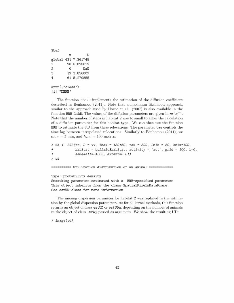
$buf

n D

global 431 7.361745

1 20 5.825619

2 0 NaN

3 19 3.856009

4 61 5.270855

attr(,"class")

[1] "DBRB"

The function BRB.D implements the estimation of the diffusion coefficientdescribed in Benhamou (2011). Note that a maximum likelihood approach,similar to the approach used by Horne et al. (2007) is also available in thefunction BRB.likD. The values of the diffusion parameters are given in m2.s−1.Note that the number of steps in habitat 2 was to small to allow the calculationof a diffusion parameter for this habitat type. We can then use the functionBRB to estimate the UD from these relocations. The parameter tau controls thetime lag between interpolated relocations. Similarly to Benhamou (2011), weset τ = 5 min, and hmin = 100 metres:

> ud <- BRB(tr, D = vv, Tmax = 180*60, tau = 300, Lmin = 50, hmin=100,

+ habitat = buffalo$habitat, activity = "act", grid = 100, b=0,

+ same4all=FALSE, extent=0.01)

> ud



Smoothing parameter estimated with a BRB-specified parameter



The missing dispersion parameter for habitat 2 was replaced in the estima-tion by the global dispersion parameter. As for all kernel methods, this functionreturns an object of class estUD or estUDm, depending on the number of animalsin the object of class ltraj passed as argument. We show the resulting UD:

> image(ud)

43

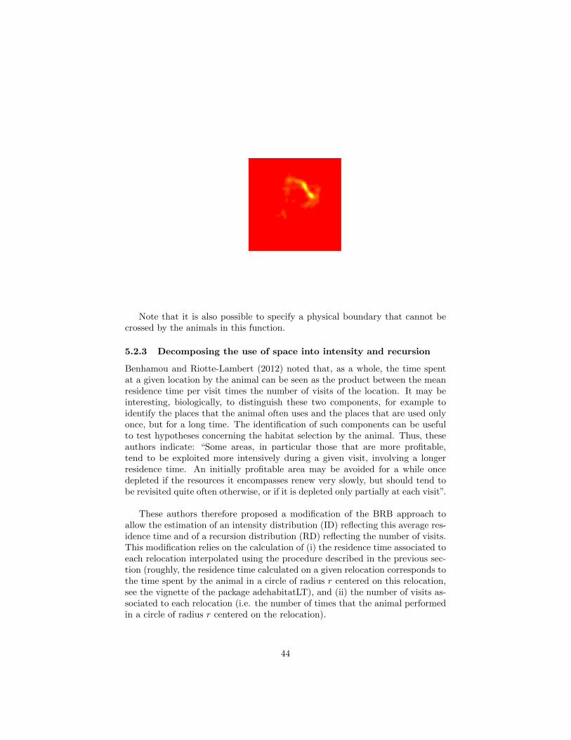
Note that it is also possible to specify a physical boundary that cannot becrossed by the animals in this function.

5.2.3 Decomposing the use of space into intensity and recursion

Benhamou and Riotte-Lambert (2012) noted that, as a whole, the time spentat a given location by the animal can be seen as the product between the meanresidence time per visit times the number of visits of the location. It may beinteresting, biologically, to distinguish these two components, for example toidentify the places that the animal often uses and the places that are used onlyonce, but for a long time. The identification of such components can be usefulto test hypotheses concerning the habitat selection by the animal. Thus, theseauthors indicate: “Some areas, in particular those that are more profitable,tend to be exploited more intensively during a given visit, involving a longerresidence time. An initially profitable area may be avoided for a while oncedepleted if the resources it encompasses renew very slowly, but should tend tobe revisited quite often otherwise, or if it is depleted only partially at each visit”.

These authors therefore proposed a modification of the BRB approach toallow the estimation of an intensity distribution (ID) reflecting this average res-idence time and of a recursion distribution (RD) reflecting the number of visits.This modification relies on the calculation of (i) the residence time associated toeach relocation interpolated using the procedure described in the previous sec-tion (roughly, the residence time calculated on a given relocation corresponds tothe time spent by the animal in a circle of radius r centered on this relocation,see the vignette of the package adehabitatLT), and (ii) the number of visits as-sociated to each relocation (i.e. the number of times that the animal performedin a circle of radius r centered on the relocation).

44

The function BRB allows to calculate the ID and RD thanks to its argumenttype. For example, consider again the dataset buffalo used in the previoussection. To estimate the ID or the RD, we have to specify:

• The diffusion parameter D: based on the elements given in the previoussection, we assumed a parameter D = 7.36. For the sake of conciseness,we define a unique diffusion parameter for all habitats;

• As in the previous section, we set Tmax = 180 min and Lmin = 50 m,hmin = 100 m, and tau = 300 seconds;

• The radius of the circle used to calculate the residence time and the numberof visits was set to 3*hmin = 300 m, as in Benhamou and Riotte-Lambert(2012);

• The time maxt used to calculate the residence time (see the help page ofthis function in the package adehabitatLT, and the vignette of this pack-age) and the number of visits, i.e. the maximum time threshold that theanimal is allowed to spend outside the patch before that we consider thatthe animal actually left the patch, was set to 2 hours, as in Benhamouand Riotte-Lambert (2012).

We estimate the UD, ID and RD with these parameters below:

> id <- BRB(buffalo$traj, D = 7.36, Tmax = 3*3600, Lmin = 50, type = "ID",

+ hmin=100, radius = 300, maxt = 2*3600, tau = 300,

+ grid = 100, extent=0.1)

> rd <- BRB(buffalo$traj, D = 7.36, Tmax = 3*3600, Lmin = 50, type = "RD",



> ud <- BRB(buffalo$traj, D = 7.36, Tmax = 3*3600, Lmin = 50, type = "UD",



> par(mfrow = c(2,2), mar=c(0,0,2,0))

> vid <- getvolumeUD(id)

> image(vid)

> contour(vid, add=TRUE, nlevels=1, levels=30,

+ lwd=3, drawlabels=FALSE)

> title("ID")

> vrd <- getvolumeUD(rd)

> image(vrd)

> contour(vrd, add=TRUE, nlevels=1, levels=30,


> title("RD")

45

> vud <- getvolumeUD(ud)

> image(vud)

> contour(vud, add=TRUE, nlevels=1, levels=95,


> title("UD")

Note that we used the function getvolumeUD for a clearer display of theresults. Remember from section 4.5.2 that this function modifies the UD com-ponent of the object passed as argument, so that the value of a pixel is equal tothe percentage of the smallest home range containing this pixel. Here, we alsodisplay the 30% isopleth calculated from the ID and RD distributions, using thefunction contour, as well as the 95% isopleth for the UD (following here therecommendations of Benhamou and Riotte-Lambert 2012). In the case of theID, the contour limits allow to identify those patches where the animal spent along time in average, and in the case of the RD, those places that the animalvisited often. A comparison of the environmental composition at these placesand in the 95% home-range estimated from the UD would allow to identifythe environmental characteristics that affect both the speed of the animal andthe number of visits he performs in a patch (see the vignette of the packageadehabitatHS for additionnal details about this kind of analysis).

5.3 The product kernel algorithm

5.3.1 Description

Until now, we have only considered utilization distribution in space. However,Horne et al. (2007) noted that it could also be useful to explore utilization distri-butions in space and time. That is, to smooth the animals distribution not onlyin space, but also in time. This approach is done by placing a three dimensional

46

kernel function (X and Y coordinates, and date) over each relocation, and then,by summing these kernel functions. The three-dimensional kernel function Kcorrespond to the combination of three one-dimensional kernel functions Kj :

K(x) =1

hxhyht

n∑i=1

3∏j=1

Kj

(xj −Xij

hj

)where hx, hy, ht are the smoothing parameters for the X, Y and time dimension,n is the number of relocations, and Xij is the coordinate of the ith relocationon the jth dimension (X,Y or time).

This method is implemented in the function kernelkc of the package ade-

habitatHR. The univariate kernel functions associated to the spatial coordinatesare the biweight kernel, that is:

K(vi) =15

16(1− v2i )2

when vi < 1 and 0 otherwise. For the time, the user has the choice betweentwo kernel functions. Either the time is considered to be a linear variable, andthe biweight kernel is used, or the time is considered to be a circular variable(e.g. January 3th 2001 is considered to be the same date as January 3th 2002 andJanuary 3th 2003, etc.) and the wrapped Cauchy kernel is used. The wrappedCauchy kernel is:

K(vi) =h(1− (1− h)2

)2π (1 + (1− h)2 − 2(1− h) cos(vih))

where 0 < h < 1.

5.3.2 Application

We now illustrate the product kernel algorithm on an example. We load thebear dataset. This dataset describes the trajectory of a brown bear monitoredusing GPS (from the package adehabitatLT):

> data(bear)

> bear



* Time zone: UTC *

Regular traject. Time lag between two locs: 1800 seconds



1 W0208 W0208 1157 157 2004-04-19 16:30:00 2004-05-13 18:30:00

47

The data are stored as an object of class ltraj (see section 5.1.2). Let uscompute the UD of this bear for the date 2004-05-01. After a visual exploration,we noted that a smoothing parameter of 1000 meters for X and Y coordinates,and of 72 hours for the time returned interesting results. We can compute theUD with:

> uu <- kernelkc(bear, h = c(1000,1000,72*3600),

+ tcalc= as.POSIXct("2004-05-01"), grid=50)

> uu



Smoothing parameter estimated with a KC-specified parameter



The result is an object of class estUD, and can be managed as such (seesection 4.2). For example to see both the trajectory and the UD, we type:

> plot(bear, spixdf=uu)

To compute the 95% home-range, there is a subtlety. Note that the UDintegral over the whole plane is not equal to 1:

> sum(slot(uu,"data")[,1])*(gridparameters(uu)[1,2]^2)

[1] 5.045653e-07

48

This is because the UD is defined in space and time. That is, the integralover the X,Y and time direction is equal to 1, and not the integral over theX,Y direction at a given time t. Therefore, the 95% home range at a given timet relies on a “restandardization”:

UD′(x, y|ti) =UD(x, y, ti)∫

x′,y′ UD(x′, y′, ti)

This is done by setting to TRUE the argument standardize of the functionsgetvolumeUD or getverticeshr. Thus, to calculate the home range of the bearat this date, type:

> ver <- getverticeshr(uu, percent=95, standardize=TRUE)

> image(uu)

> plot(ver, add=TRUE)

Note that it is possible to estimate the UD at a succession of ti close in time,then to draw the images corresponding and save them in a file, and finally tocombine these images into a movie. The movie can then be explored to identifypatterns. For example, the following code can be used to generate image files(because it is very long, we do not execute it in this vignette:

> ## compute the sequence of dates at which the UD is to be

> ## estimated

> vv <- seq(min(bear[[1]]$date), max(bear[[1]]$date), length=50)

> head(vv)

> ## estimates the UD at each time point

> re <- lapply(1:length(vv), function(i) {

+

49

+ ## estimate the UD. We choose a smoothing parameter of

+ ## 1000 meters for X and Y coordinates, and of 72 hours

+ ## for the time (after a visual exploration)

+ uu <- kernelkc(bear, h = c(1000,1000,72*3600),

+ tcalc= vv[i], grid=50)

+

+ ## To save the result in a file, type

+ jpeg(paste("UD", i, ".jpg", sep=""))

+

+

+ ## draw the image

+ image(uu, col=grey(seq(1,0,length=10)))

+ title(main=vv[i])

+

+ ## highlight the 95 percent home range

+ ## we set standardize = TRUE because we want to estimate

+ ## the home range in space from a UD estimated in space and

+ ## time

+ plot(getverticeshr(uu, 95, standardize=TRUE), lwd=2,

+ border="red", add=TRUE)

+

+ ## close the device

+ dev.off()

+ })

The images can then be combined using the program mencoder (Linux) orImageMagick (Windows). For Linux users, the following command line can beused:

mencoder mf://*.jpg -mf w=320:h=240:fps=15:type=jpeg -ovc lavc -o UD.avi

5.3.3 Application with time considered as a circular variable

Now, consider the time as a circular variable. We consider a time cycle of 24hour. We will estimate the UD at 03h00. We have to define the beginning ofthe cycle (argument t0 of the function kernelkc). We consider that the timecycle begins at midnight (there is no particular reason, it is just to illustratethe function). We have to set, as the argument t0, any object of class POSIXctcorresponding to a date at this hour, for example the 12/25/2012 at 00H00:

> t0 <- as.POSIXct("2012-12-25 00:00")

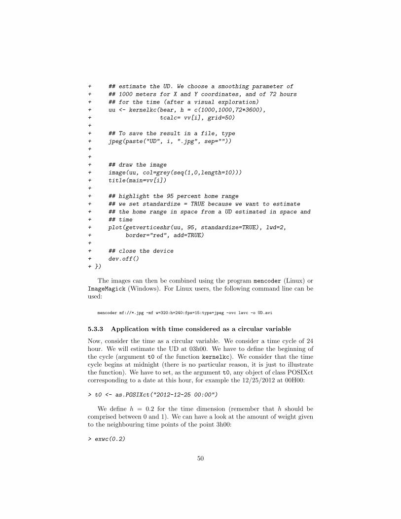
We define h = 0.2 for the time dimension (remember that h should becomprised between 0 and 1). We can have a look at the amount of weight givento the neighbouring time points of the point 3h00:

> exwc(0.2)

50

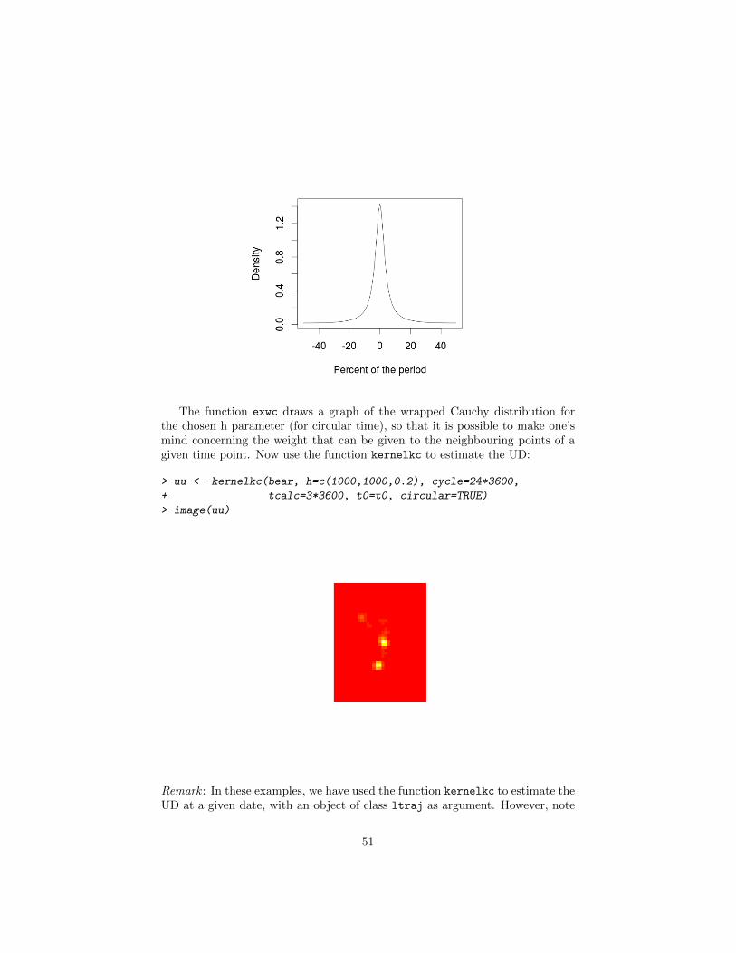
The function exwc draws a graph of the wrapped Cauchy distribution forthe chosen h parameter (for circular time), so that it is possible to make one’smind concerning the weight that can be given to the neighbouring points of agiven time point. Now use the function kernelkc to estimate the UD:

> uu <- kernelkc(bear, h=c(1000,1000,0.2), cycle=24*3600,

+ tcalc=3*3600, t0=t0, circular=TRUE)

> image(uu)

Remark : In these examples, we have used the function kernelkc to estimate theUD at a given date, with an object of class ltraj as argument. However, note

51

that the product kernel algorithm can be used on other kind of data. Thus, thefunction kernelkcbase accepts as argument a data frame with three columns(x, y and time). The example section on the help page of this function providesexamples of use.

6 Convex hulls methods

Several methods relying on the calculation of multiple convex hulls have beendeveloped to estimate the home range from relocation data. The package ade-

habitatHR implements three such methods. I describe these three methods inthis section.

Remark: note that the function getverticeshr is generic, and can be used forall home-range estimation methods of the package adehabitatHR (except forthe minimum convex polygon).

6.1 The single linkage algorithm

6.1.1 The method

Kenward et al. (2001) proposed a modification of the single-linkage cluster anal-ysis for the estimation of the home range. Whereas this method does not relyon a probabilistic definition of the home range (contrary to the kernel method),it can still be useful to identify the structure of the home range.

The clustering process is the following (also described on the help page ofthe function clusthr): the three locations with the minimum mean of nearest-neighbour joining distances (NNJD) form the first cluster. At each step of theclustering process, two distances are computed: (i) the minimum mean NNJDbetween three locations (which corresponds to the next potential cluster) and(ii) the minimum of the NNJD between a cluster ”c” and the closest location. If(i) is smaller that (ii), another cluster is defined with these three locations. If(ii) is smaller than (i), the cluster ”c” gains a new location. If this new locationbelong to another cluster, the two cluster fuses. The process stop when all re-locations are assigned to the same cluster.

At each step of the clustering process, the proportion of all relocations whichare assigned to a cluster is computed (so that the home range can be definedto enclose a given proportion of the relocations at hand, i.e. to an uncompleteprocess). At a given step, the home range is defined as the set of minimumconvex polygons enclosing the relocations in the clusters.

52

6.1.2 The function clusthr

Take as example the puechabonsp dataset:

> uu <- clusthr(puechabonsp$relocs[,1])

> class(uu)

[1] "MCHu"

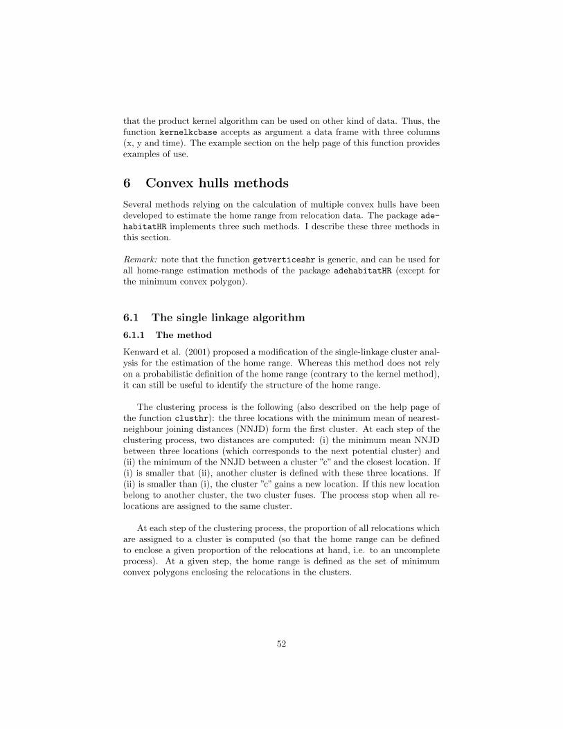
The class MCHu is returned by all the home range estimation methods basedon clustering methods (LoCoH and single linkage). The object uu is basicallya list of SpatialPolygonsDataFrame objects (one per animal). We can have adisplay of the home ranges by typing:

> plot(uu)

The information stored in each SpatialPolygonsDataFrame object is thefollowing (for example, for the third animal):

> as.data.frame(uu[[3]])

percent area

1 7.5 0.02505

2 15.0 0.06240

3 22.5 0.11930

4 30.0 0.17420

5 37.5 0.18520

6 37.5 1.18020

7 40.0 1.62740

8 40.0 2.52375

53

9 42.5 3.05210

10 50.0 3.28650

11 50.0 3.71345

12 52.5 4.10105

13 55.0 4.85180

14 55.0 5.79000

15 57.5 6.70530

16 60.0 6.98955

17 67.5 7.66045

18 75.0 8.08420

19 77.5 9.33975

20 77.5 13.27250

21 77.5 30.72235

22 80.0 32.28935

23 82.5 37.80750

24 85.0 37.80750

25 87.5 43.34810

26 90.0 44.71795

27 90.0 64.17895

28 92.5 68.91885

29 95.0 71.93205

30 97.5 100.12995

31 100.0 162.84550

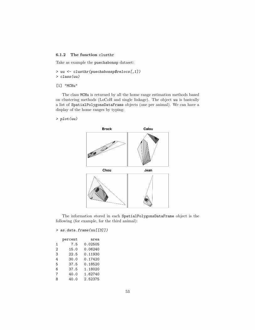
From this data frame, it is possible to extract a home range corresponding toa particular percentage of relocations enclosed in the home range. For example,the smallest home range enclosing 90% of the relocations corresponds to the row26 of this data frame:

> plot(uu[[3]][26,])

54

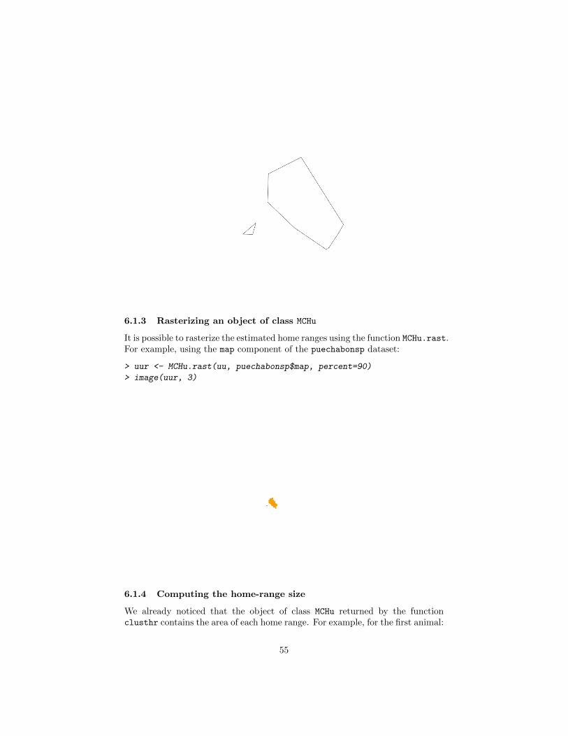
6.1.3 Rasterizing an object of class MCHu

It is possible to rasterize the estimated home ranges using the function MCHu.rast.For example, using the map component of the puechabonsp dataset:

> uur <- MCHu.rast(uu, puechabonsp$map, percent=90)

> image(uur, 3)

6.1.4 Computing the home-range size

We already noticed that the object of class MCHu returned by the functionclusthr contains the area of each home range. For example, for the first animal:

55

> head(as.data.frame(uu[[1]]))

percent area

1 10.00000 0.01790

2 13.33333 0.04565

3 23.33333 0.06635

4 26.66667 0.09470

5 36.66667 0.27170

6 36.66667 0.79285

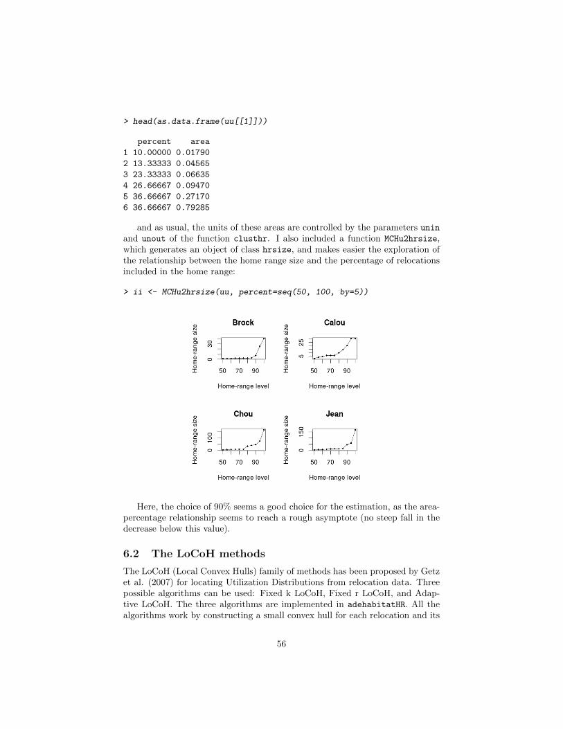
and as usual, the units of these areas are controlled by the parameters uninand unout of the function clusthr. I also included a function MCHu2hrsize,which generates an object of class hrsize, and makes easier the exploration ofthe relationship between the home range size and the percentage of relocationsincluded in the home range:

> ii <- MCHu2hrsize(uu, percent=seq(50, 100, by=5))

Here, the choice of 90% seems a good choice for the estimation, as the area-percentage relationship seems to reach a rough asymptote (no steep fall in thedecrease below this value).

6.2 The LoCoH methods

The LoCoH (Local Convex Hulls) family of methods has been proposed by Getzet al. (2007) for locating Utilization Distributions from relocation data. Threepossible algorithms can be used: Fixed k LoCoH, Fixed r LoCoH, and Adap-tive LoCoH. The three algorithms are implemented in adehabitatHR. All thealgorithms work by constructing a small convex hull for each relocation and its

56

neighbours, and then incrementally merging the hulls together from smallest tolargest into isopleths. The 10% isopleth contains 10% of the points and repre-sents a higher utilization than the 100% isopleth that contains all the points (asfor the single linkage method). I describe the three methods below (this descrip-tion is also on the help page of the functions LoCoH.k, LoCoH.r and LoCoH.a):

• Fixed k LoCoH: Also known as k-NNCH, Fixed k LoCoH is described inGetz and Willmers (2004). The convex hull for each point is constructedfrom the (k-1) nearest neighbors to that point. Hulls are merged togetherfrom smallest to largest based on the area of the hull. This method isimplemented in the function LoCoH.k;

• Fixed r LoCoH: In this case, hulls are created from all points within rdistance of the root point. When merging hulls, the hulls are primarilysorted by the value of k generated for each hull (the number of pointscontained in the hull), and secondly by the area of the hull. This methodis implemented in the function LoCoH.r;

• Adaptive LoCoH: Here, hulls are created out of the maximum nearestneighbors such that the sum of the distances from the nearest neighborsis less than or equal to d. Use the same hull sorting as Fixed r LoCoH.This method is implemented in the function LoCoH.a;

All of these algorithms can take a significant amount of time.

Note: these functions rely on the availability of the packages rgeos and gpclib,which may not be available for all OS (especially MacOS).

6.3 Example with the Fixed k LoCoH method

We use the fixed k LoCoH method to estimate the home range of the wild boarsmonitored at Puechabon, for example with k = 5:

> res <- LoCoH.k(puechabonsp$relocs[,1], 10)

The object returned by the function is of the class MCHu, as the objectsreturned by the function clusthr (see previous section). Consequently, all thefunctions developed for this class of objects can be used (including rasterizationwith MCHu.rast, computation of home-range size with MCHu2hrsize, etc.). Avisual display of the home ranges can be obtained with:

> plot(res)

Note that the relationship between the home range size and the number ofchosen neighbours can be investigated thanks to the function LoCoH.k.area:

57

> LoCoH.k.area(puechabonsp$relocs[,1], krange=seq(4, 15, length=5),

+ percent=100)

Just copy and paste the above code (it is not executed in this report). Anasymptote seems to be reached at about 10 neighbours, which justifies the choiceof 10 neighbours for an home range estimated with 100% of the relocations (amore stable home range size).

6.4 The characteristic hull method

Downs and Horner (2009) developed an interesting method for the home rangeestimation. This method relies on the calculation of the Delaunay triangulationof the set of relocations. Then, the triangles are ordered according to their area(and not their perimeter). The smallest triangles correspond to the areas themost intensively used by the animals. It is then possible to derive the homerange estimated for a given percentage level.

For example, consider the puechabonsp dataset.

> res <- CharHull(puechabonsp$relocs[,1])

> class(res)

[1] "MCHu"

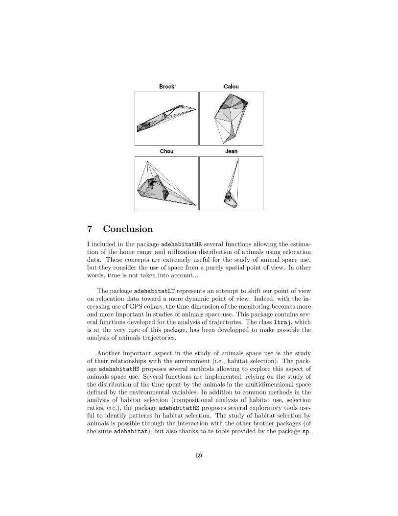
The object returned by the function is also of the class MCHu, as the ob-jects returned by the functions clusthr and LoCoH.* (see previous sections).Consequently, all the functions developed for this class of objects can be used(including rasterization with MCHu.rast, computation of home-range size withMCHu2hrsize, extraction of the home-range contour with getverticeshr etc.).A visual display of the home ranges can be obtained with:

> plot(res)

58

7 Conclusion

I included in the package adehabitatHR several functions allowing the estima-tion of the home range and utilization distribution of animals using relocationdata. These concepts are extremely useful for the study of animal space use,but they consider the use of space from a purely spatial point of view. In otherwords, time is not taken into account...

The package adehabitatLT represents an attempt to shift our point of viewon relocation data toward a more dynamic point of view. Indeed, with the in-creasing use of GPS collars, the time dimension of the monitoring becomes moreand more important in studies of animals space use. This package contains sev-eral functions developed for the analysis of trajectories. The class ltraj, whichis at the very core of this package, has been developped to make possible theanalysis of animals trajectories.

Another important aspect in the study of animals space use is the studyof their relationships with the environment (i.e., habitat selection). The pack-age adehabitatHS proposes several methods allowing to explore this aspect ofanimals space use. Several functions are implemented, relying on the study ofthe distribution of the time spent by the animals in the multidimensional spacedefined by the environmental variables. In addition to common methods in theanalysis of habitat selection (compositional analysis of habitat use, selectionratios, etc.), the package adehabitatHS proposes several exploratory tools use-ful to identify patterns in habitat selection. The study of habitat selection byanimals is possible through the interaction with the other brother packages (ofthe suite adehabitat), but also thanks to te tools provided by the package sp,

59

which allow to handle raster and vector maps of environmental variables. Notethat the package adehabitatMA provides additionnal tools which can be usefulin the particular field of habitat selection study.

References

Bullard, F. 1999. Estimating the home range of an animal: a Brownian bridgeapproach. Johns Hopkins University. Master thesis.

Burt, W.H. 1943. Territoriality and home range concepts as applied to mam-mals. Journal of Mammalogy, 24, 346-352.

Benhamou, S. and Cornelis, D. 2010. Incorporating movement behavior andbarriers to improve kernel home range space use estimates. Journal ofWildlife Management, 74, 1353–1360.

Benhamou, S. and Riotte-Lambert, L. 2012. Beyond the Utilization Distri-bution: Identifying home range areas that are intensively exploited orrepeatedly visited. Ecological Modelling, 227, 112-116.

Benhamou, S. 2011. Dynamic approach to space and habitat use based onbiased random bridges. PLOS ONE, 6, 1–8.

Calenge, C. 2005. Des outils statistiques pour l’analyse des semis de pointsdans l’espace ecologique. Universite Claude Bernard Lyon 1.

Calenge, C. 2006. The package adehabitat for the R software: a tool for theanalysis of space and habitat use by animals. Ecological modelling, 197,516–519.

Calenge, C., Dray, S. and Royer-Carenzi, M. 2009. The concept of animalstrajectories from a data analysis perspective. Ecological Informatics, 4,34-41.

Downs, J.A. and Horner, M.W. 2009. A Characteristic-Hull Based Method forHome Range Estimation. Transactions in GIS, 13: 527–537.

Getz, W., Fortmann-Roe, S., Cross, P., Lyons, A., Ryan, S. and Wilmers, C.2007. LoCoH: Nonparameteric Kernel Methods for Constructing HomeRanges and Utilization Distributions. PloS one, 2, e207.

Horne, J.S., Garton, E.O., Krone, S.M. and Lewis, J.S. 2007. Analyzing animalmovements using Brownian bridges. Ecology, 88, 2354–2353.

Keating, K. and Cherry, S. 2009. Modeling utilization distributions in spaceand time Ecology, 90, 1971-1980.

Kenward, R., Clarke, R., Hodder, K. and Walls, S. 2001. Density and linkageestimators of home range: nearest neighbor clustering defines multinuclearcores. Ecology, 82, 1905–1920.

60

Maillard, D. 1996. Occupation et utilisation de la garrigue et du vigno-ble mediterraneens par le sanglier (Sus scrofa L.). Universite de droit,d’economie et des sciences d’Aix-Marseille III, PhD thesis.

Mohr, C. 1947. Table of equivalent populations of North American small mam-mals. American Midland Naturalist, 37, 223–249.

Pebesma, E. and Bivand, R.S. 2005. Classes and Methods for Spatial data inR. R News, 5, 9–13.

Silverman, B. 1986. Density estimation for statistics and data analysis. Chap-man and Hall, London.

van Winkle, W. (1975) Comparison of several probabilistic home-range models.Journal of Wildlife Management, 39, 118–123.

Wand, M. and Jones, M. 1995. Kernel smoothing. Chapman and Hall/CRC.

Worton, B. 1989. Kernel methods for estimating the utilization distribution inhome-range studies. Ecology, 70, 164–168.

61

Home Range Estimation in R: the adehabitatHR Package

Documents

Transcript of Home Range Estimation in R: the adehabitatHR Package