Home Productivity

Benjamin Bridgman∗

Bureau of Economic Analysis

February 2013

Abstract

This paper examines the productivity of home production. I calculate annual home produc-

tion output and productivity for the United States from 1929 to 2010. Both labor and total

factor productivity increased rapidly after World War Two, but slowed after the late 1970s.

The household sector is capital intensive due to the importance of residential capital. The

capital intensity increased in the late 1970s due to increased consumer durables holdings.

JEL classification: O3.

Keywords: Home production; Labor productivity; Total factor productivity.

∗I thank Ryan Greenaway-McGrevy, Matt Osborne and Todd Schoellman for comments. The views expressed

in this paper are solely those of the author and not necessarily those of the U.S. Bureau of Economic Analysis

or the U.S. Department of Commerce. Address: U.S. Department of Commerce, Bureau of Economic Analysis,

Washington, DC 20230. email: Benjamin.Bridgman@bea.gov. Tel. (202) 606-9991. Fax (202) 606-5366.

1

1 Introduction

A large theoretical literature has found that the addition of a home production sector improves

the predictions of macroeconomic models1. It continues to be an area of active research. For

example, a recent literature has examined the effect of productivity growth on changes in the

industrial structure of the economy. (See Herrendorf, Rogerson & Valentinyi (2012) for a sur-

vey.) Kongsamut, Rebelo & Xie (2001) and Buera & Kaboski (2012b) feature neutral technical

change and non-homothetic preferences while Ngai & Pissarides (2007) feature differences in

technical change across sectors. Other theories, such as Acemoglu & Guerrieri (2008), rely on

differing factor shares in production. Determining what forces are at work requires data on

factor shares and technical change in home production.

However, little is known about the household sector’s basic inner workings since prac-

tical considerations caused economic statisticians to exclude it from the National Income and

Product Accounts (NIPAs)2. Models must be parameterized without the discipline of data.

Rather, the models are used to back out what is going on in this sector (Ingram, Kocherlakota

& Savin 1997). In a recent example, Rogerson (2008) argues that the household sector is es-

sential to understanding different labor market outcomes in the United States compared to

Europe. Since “measures of home sector productivity do not exist,” he must use an imprecisely

estimated elasticity parameter to back out this productivity.

This paper generates a number of facts about the household sector to guide macroe-

conomic modeling, with an emphasis on productivity measurement. Improvements in the

measurement of time use, such as the regular collection of time use data through the American

1Important contributions include Benhabib, Rogerson & Wright (1991) and Greenwood & Hercowitz (1991)

on business cycles, Parente, Rogerson & Wright (2000) on the welfare costs of growth distortions and Rupert,

Rogerson & Wright (2000) on labor supply elasticities. Greenwood, Rogerson & Wright (1995) surveys its

inclusion in macroeconomic models. Recent work includes Aruoba, Davis & Wright (2012) and Aguiar, Hurst &

Karabarbounis (2011).2It was a concern during the original work on national income measurement (Kuznets 1934). See Gronau

(1986) and Gronau (1997) for surveys of more recent work.

2

Time Use Study (ATUS), have led to better estimates of the output of this sector. Build-

ing on work done by researchers at the Bureau of Economic Analysis (BEA) (Landefeld

& McCulla 2000, Landefeld, Fraumeni & Vojtech 2009, Bridgman, Dugan, Lal, Osborne &

Villones 2012), I estimate annual home production for the United States from 1929 to 2010

using national income accounting principles. I then examine labor and total factor productivity

(TFP) in this sector.

I find that home production has generally declined in importance compared to mea-

sured GDP. However during the dislocations of the Great Depression and World War Two, its

importance fluctuated significantly. The ratio of home production to measured GDP increased

to 85 percent in the depths of the depression (1932) and dropped to 43 percent during the

height of the war (1943). The estimates help fill in the historical record on the size of home

production by providing the better part of a century of consistent data. Other such estimates

include Eisner (1989) and Folbre & Wagman (1993).

Home productivity grew at a rate similar to that of the market economy in the postwar

period until the 1970s. Home labor productivity grew an average of 2.0 percent a year during

the period 1948-1977, very similar to the 2.1 percent in market. There is a severe slowdown in

home productivity in the late 1970s. Labor productivity was nearly flat, growing an average of

only 0.02 percent from 1978 to 2010. In contrast, market labor productivity grew 1.6 percent

annually.

There has been significant shifts in how the home sector produces output. While the

household sector has always been capital intensive due to the importance of residential capital,

labor has been progressively replaced by capital since 1978. Capital share drops from 0.5

to 0.37. Most of this increase is due to consumer durables becoming much more important.

This large change in capital share suggests that the household sector’s production function

must allow for substitutability between capital and labor, such as the CES form proposed by

Greenwood & Hercowitz (1991).

TFP grows 1.3 percent annually from 1929 to 2010. This growth has not been uniform.

3

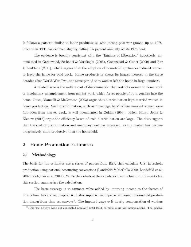
It follows a pattern similar to labor productivity, with strong post-war growth up to 1978.

Since then TFP has declined slightly, falling 0.5 percent annually off its 1978 peak.

The evidence is broadly consistent with the “Engines of Liberation” hypothesis, an-

nunciated in Greenwood, Seshadri & Yorukoglu (2005), Greenwood & Guner (2009) and Bar

& Leukhina (2011), which argues that the adoption of household appliances induced women

to leave the home for paid work. Home productivity shows its largest increase in the three

decades after World War Two, the same period that women left the home in large numbers.

A related issue is the welfare cost of discrimination that restricts women to home work

or involuntary unemployment from market work, which forces people of both genders into the

home. Jones, Manuelli & McGrattan (2003) argue that discrimination kept married women in

home production. Such discrimination, such as “marriage bars” where married women were

forbidden from market work, is well documented in Goldin (1990). Hsieh, Hurst, Jones &

Klenow (2012) argue the efficiency losses of such discrimination are large. The data suggest

that the cost of discrimination and unemployment has increased, as the market has become

progressively more productive than the household.

2 Home Production Estimates

2.1 Methodology

The basis for the estimates are a series of papers from BEA that calculate U.S. household

production using national accounting conventions (Landefeld & McCulla 2000, Landefeld et al.

2009, Bridgman et al. 2012). While the details of the calculation can be found in those articles,

this section summarizes the calculation.

The basic strategy is to estimate value added by imputing income to the factors of

production: labor L and capital K. Labor input is uncompensated hours in household produc-

tion drawn from time use surveys3. The imputed wage w is hourly compensation of workers

3Time use surveys were not conducted annually until 2003, so most years are interpolations. The general

4

employed in the household sector, under the assumption that market and non-market workers

have the same marginal product of labor in the home. There are three types of capital used

by the household: consumer durables, residential capital and governmental capital provided

to the household and used in production4. The capital services are the asset rate of return rj

for each type of capital plus depreciation δj , for j ∈ {Durables,Residential,Government}.

The rate of returns used are households’ financial asset returns for durables, imputed rents for

residential and government debt returns for government capital. Formally, household output

Y is given by:

Y = C + I = wL+∑j

[(rj + δj)Kj + Ij ] (2.1)

Note that several components, such as the services of residential capital and investment

in household capital, are already included in measured GDP. Therefore, home production is

not purely an addition to measured GDP. Home productivity will include all household output,

not just the new imputations.

The BEA estimates cover the period 1946 to 2010. This paper extends them back

to 1929 using as similar methodology as possible. (Details on the data are reported in the

Appendix.) There are two main differences in the calculation for the 1929 to 1945 period.

First, I use the home production hours estimates from Ramey (2009) and Ramey & Francis

(2009) as the measure of labor hours5. Second, the capital return series used to impute capital

services of consumer durables in the BEA estimates does not exist for the earlier period. Instead

I use the Moody’s Seasoned Baa Corporate Bond Yield. Both series overlap with the BEA data.

methodology is to disaggregate hours data in survey years by demographic group then project non-survey years

using data on population size of those groups.4Governmental capital is half of the “Highways and streets” category of government capital. Half is chosen

based on a 2000 survey road use that found that half of car passenger milage was accounted for by non-commuting

household travel. Using the 2000 share for the whole period is arbitrary, but has very little quantitative impact

since government capital services are tiny.5I generate total hours by multiplying their estimate of average weekly hours by the population and 52 (the

number of weeks in a year).

5

They give very similar estimates. I discuss the robustness of the estimates below.

2.2 Home Production 1929-2010

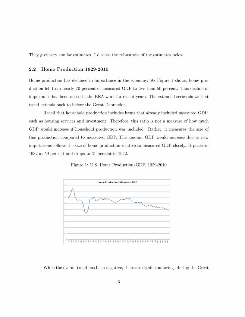
Home production has declined in importance in the economy. As Figure 1 shows, home pro-

duction fell from nearly 70 percent of measured GDP to less than 50 percent. This decline in

importance has been noted in the BEA work for recent years. The extended series shows that

trend extends back to before the Great Depression.

Recall that household production includes items that already included measured GDP,

such as housing services and investment. Therefore, this ratio is not a measure of how much

GDP would increase if household production was included. Rather, it measures the size of

this production compared to measured GDP. The amount GDP would increase due to new

imputations follows the size of home production relative to measured GDP closely. It peaks in

1932 at 59 percent and drops to 31 percent in 1942.

Figure 1: U.S. Home Production/GDP, 1929-2010

0

0.1

0.2

0.3

0.4

0.5

0.6

0.7

0.8

0.9

1929

1931

1933

1935

1937

1939

1941

1943

1945

1947

1949

1951

1953

1955

1957

1959

1961

1963

1965

1967

1969

1971

1973

1975

1977

1979

1981

1983

1985

1987

1989

1991

1993

1995

1997

1999

2001

2003

2005

2007

2009

Home Production/Measured GDP

While the overall trend has been negative, there are significant swings during the Great

6

Depression and World War Two. Home production did not fall as much as the rest of the

economy during the Depression making it almost are big as measured GDP. Market hours far

significantly while household production hours increase slightly (Ramey 2009).

The opposite happens during the war, where home production drops to its lowest per-

centage of GDP in the series. This shift largely reflects the recovery in the market sector. It

also reflects restriction on the production of home capital as production was geared to war

materiel. The movement of women into the defense industries and out of the home, the “Rosie

the Riveter” (real name: Bernice Olsen) effect, is minor. Women’s average hours in home

production does not fall much6.

3 Labor Productivity

To measure productivity, we need to deflate the nominal household output to put it in real

terms. As a baseline, I use the price index for private household output. This sector is

comprised of the services of owner-occupied housing and the compensation paid to domestic

workers. This measure is the closest to the concept of household production in the published

NIPAs. I discuss the robustness of this choice below.

Figure 2 shows labor productivity in home production, as measured by real value added

per hour. Productivity increased rapidly after World War Two until the late 1970s, growing

an average of 2.0 percent a year from 1948-1977. This rate is similar to that of the market

economy, which 2.1 percent per over the same period7. It is flat both during the depression

and war and after 1978. Home productivity only grew an average of only 0.02 percent from

1978 to 2010 while market labor productivity grew 1.6 percent per year.

The home sector is less productive than the rest of the economy, a gap that has been

6As documented in Goldin & Olivetti (2013), World War Two had an impact on women’s labor participation

after the war.7Labor productivity is measured as GDP per hour using BEA’s measure of total market hours: NIPA Table

6.9, line 1.

7

Figure 2: Labor Productivity in Home Production 1929-2010

0

5

10

15

20

25

30

1929

1931

1933

1935

1937

1939

1941

1943

1945

1947

1949

1951

1953

1955

1957

1959

1961

1963

1965

1967

1969

1971

1973

1975

1977

1979

1981

1983

1985

1987

1989

1991

1993

1995

1997

1999

2001

2003

2005

2007

2009

Labor Productivity in Home Production

increasing. Figure 3 shows the ratio of home productivity to real GDP per market hour worked.

In addition to the BEA hours used above, I use market labor hours are calculated as average

work week from Ramey (2009) times the population times 52, the number of weeks. This

measure is broadly consistent with the BEA measure, but has a higher level. Therefore, labor

productivity is lower with the Ramey (2009) hours. Since neither series has full coverage of the

sample period (Ramey (2009) ends in 2005 and the BEA data begin in 1948) so I report both.

After the low ebb of the Depression and the war, an hour of home production produced

nearly as many dollars of value added compared to the economy measured by GDP (using

the Ramey (2009) hours). No matter which hours are used, the home sector has become

relatively less productive since then. In 2005, an hour of work produced $23.69 of value added

compared to $44.19 for market work (using the Ramey (2009) hours). This finding supports

the assumption in Nosal, Rogerson & Wright (1992) that workers would prefer to work in the

market.

The data suggest that the economic cost of distortions, such as discrimination (Goldin

8

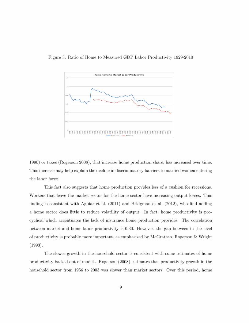
Figure 3: Ratio of Home to Measured GDP Labor Productivity 1929-2010

0

0.2

0.4

0.6

0.8

1

1.2

1929

1931

1933

1935

1937

1939

1941

1943

1945

1947

1949

1951

1953

1955

1957

1959

1961

1963

1965

1967

1969

1971

1973

1975

1977

1979

1981

1983

1985

1987

1989

1991

1993

1995

1997

1999

2001

2003

2005

2007

2009

Ratio Home to Market Labor Productivity

Ramey hours BEA hours

1990) or taxes (Rogerson 2008), that increase home production share, has increased over time.

This increase may help explain the decline in discriminatory barriers to married women entering

the labor force.

This fact also suggests that home production provides less of a cushion for recessions.

Workers that leave the market sector for the home sector have increasing output losses. This

finding is consistent with Aguiar et al. (2011) and Bridgman et al. (2012), who find adding

a home sector does little to reduce volatility of output. In fact, home productivity is pro-

cyclical which accentuates the lack of insurance home production provides. The correlation

between market and home labor productivity is 0.30. However, the gap between in the level

of productivity is probably more important, as emphasized by McGrattan, Rogerson & Wright

(1993).

The slower growth in the household sector is consistent with some estimates of home

productivity backed out of models. Rogerson (2008) estimates that productivity growth in the

household sector from 1956 to 2003 was slower than market sectors. Over this period, home

9

productivity grew 0.8 percent a year compared to 1.8 for the market sector (using BEA hours).

4 Total Factor Productivity

This section examines total factor productivity (TFP) in the household sector. This calcula-

tion requires taking a stand on how capital and labor are combined. I begin by examining

what production functions are consistent with data. I show the evidence is consistent with a

production function that allows for substitutability between capital and labor, such as the CES

function. I then calculate TFP using a labor augmenting CES function.

4.1 Production Function

Since there is little data on home production, we have little direct evidence on what the

appropriate home production function is. As a result, there is no consensus in the literature on

what form to use. The most common production function in macroeconomics is Cobb-Douglas.

It was used by Benhabib et al. (1991) among others.

As shown in Figure 4, home production shows a significant change in labor share which

indicates that the Cobb-Douglas production function is a poor fit for the data. In the early

period, households invest very little in home capital. As discussed above, World War Two

severely restricted home investment. In the later period, the opposite is true. Households

replace labor input with capital input. As a result, the labor share of the sector declines.

Home production is capital intensive, and has become more so over time. Labor share

falls from 0.50 in 1929 to 0.37 in 2010. This high capital intensity is due to the large stock

of residential capital. Consumer durables have become more important, increasing from 5.5 to

21.6 percent of real home capital held by the household from 1929 to 2010.

Given the change in factor shares, a more promising form is a CES production function

that allows for more flexible substitution between inputs. (It collapses to Cobb-Douglas when

the capital-labor elasticity is equal to one). A difficulty with this form is that the productivity

10

Figure 4: Labor Share in Home Production 1929-2010

0

0.1

0.2

0.3

0.4

0.5

0.6

0.7

0.8

1929

1931

1933

1935

1937

1939

1941

1943

1945

1947

1949

1951

1953

1955

1957

1959

1961

1963

1965

1967

1969

1971

1973

1975

1977

1979

1981

1983

1985

1987

1989

1991

1993

1995

1997

1999

2001

2003

2005

2007

2009

Labor Share in Home Production

process is also more flexible. Each input can have a separate productivity process, whereas in

Cobb-Douglas productivity is always Hicks-neutral. Identifying the degree of bias in technical

change has been a long standing controversy, since the capital-labor elasticity and technical

biases are not separately identified. Some structural assumption is required to proceed. (See

Leon-Ledesma, McAdam & Willman (2010) for a survey of this literature.)

As a baseline, I use labor augmenting technical change:

Yt = [θKλt + (1− θ)(AtLt)

λ]1λ (4.1)

where Yt is home production, Kt is household capital and Lt is hours of home production.

I selected this functional form since it has been used previously in the literature. For

example, it was used by Greenwood & Hercowitz (1991) and Gomme, Kydland & Rupert

(2001). The TFP calculation is not significantly changed by alternative assumptions on how

productivity enters.

11

4.2 TFP Results

Once we have selected a functional form, we have two additional tasks before we can calculate

TFP. We need a measure of real capital inputs and we need parameter values for the production

function.

As the measure of capital, I aggregate the three capital inputs (consumer durables,

residential and governmental capital) into a capital index. Since BEA’s real capital stocks are

calculated using chain weighted price indices, we cannot simply add the deflated capital series.

Following BEA’s methodology, I generated a psuedo-Fisher index of capital input8.

Finally, for baseline parameter values I use the estimates from McGrattan, Rogerson &

Wright (1997). They find that λ = 0.19 and θ = 0.22.

Line “CES TFP (Labor augmenting)” in Figure 5 shows the baseline estimate of TFP.

Over the sample period, TFP grows an average of 1.3 percent a year. There are significant

differences over time. There is little growth during the Depression. TFP grows steadily during

the postwar period prior to 1978 then flattens out. From 1945 to 1978, TFP grew 2.7 percent,

compared to -0.5 percent annually from afterward. The slowdown in TFP coincides with the

slowdown in labor productivity.

To see how sensitive the results are to the assumption on technical bias, I calculate

TFP using a Hicks neutral CES production function using the same values for θ and λ:

Yt = At[θKλt + (1− θ)(Lt)

λ]1λ (4.2)

Line “CES TFP (Hicks neutral)” in Figure 5 shows this estimate. The pattern of growth is

very similar, though the magnitude of TFP growth is smaller. The average growth rate over

the sample is 0.9 percent, compared to 1.3 percent in the baseline case. This slower growth is

seen in every subperiod. The postwar growth period (1945 to 1978) is a bit slower (2.2 percent

compared to 2.7 percent in the baseline) and the slowdown a bit worse (-0.8 percent annually

versus -0.5 percent a year).

8This methodology can be found at http://www.bea.gov/national/FA2004/Details/xls/DetailCDG.xls.

12

Figure 5: Total Factor Productivity in Home Production 1929-2010

0

50

100

150

200

250

300

350

400

1929

1931

1933

1935

1937

1939

1941

1943

1945

1947

1949

1951

1953

1955

1957

1959

1961

1963

1965

1967

1969

1971

1973

1975

1977

1979

1981

1983

1985

1987

1989

1991

1993

1995

1997

1999

2001

2003

2005

2007

2009

Home Production TFP

CES TFP (Labor Augmenting) Cobb-Douglas CES TFP (Hicks neutral)

Changing the capital-labor elasticity has a similar effect. I set λ = 1 to collapse the

CES into a Cobb-Douglas function. Again, as seen in line “Cobb-Douglas” in Figure 5, the

pattern is unchanged though the magnitudes are larger.

As shown in Figure 6, the productivity slowdown coincides with a slowdown in home

output. Capital input is exploding while output grows slowly. Since inputs are growing while

output slows, TFP will slow for most functional forms and parameters. It is only the magnitudes

that will be sensitive to such changes.

While the data are annual, productivity is pro-cyclical. The baseline TFP measure and

real GDP has a correlation of 0.45 over the period 1929 to 2010. This observation matches with

Greenwood & Hercowitz (1991) and (Fisher 2007), who use models where home and market

productivity shocks are correlated to generate the empirical co-movement of home and market

investment. The data confirm this positive correlation.

13

Figure 6: Inputs and Output in Home Production 1929-2010

0

20

40

60

80

100

120

140

1925

1927

1929

1931

1933

1935

1937

1939

1941

1943

1945

1947

1949

1951

1953

1955

1957

1959

1961

1963

1965

1967

1969

1971

1973

1975

1977

1979

1981

1983

1985

1987

1989

1991

1993

1995

1997

1999

2001

2003

2005

2007

2009

Inputs and Output in Home Production

Real HH capital (2005=100) hours index (2005=100) HH Y index (2005 = 100)

4.3 Why did productivity slow down?

Why did productivity slow in the late 1970s? The year 1978 marks a significant change in the

household sector. It is the year that labor share begins a concerted decline.

It is surprising that the shifts occur so late. The mechanism emphasized by the “Engines

of Liberation” hypothesis, the diffusion of household appliances that the allowed women to

leave the home for paid work, was well underway by the 1970s. (See Greenwood et al. (2005),

Greenwood & Guner (2009) and Bar & Leukhina (2011).) According to the Census, half of

women worked in the market in 1980 nearly double the rate in 1950 (27.1 percent)9. The binary

choice some or no market hours masks a slower increase in average hours worked by women,

especially married white women (Jones et al. 2003).

Strong productivity growth may have initially held married women in the household

sector. Households may have responded to increasing productivity by increasing home produc-

tion. The introduction of household appliances did not reduce married women’s hours and may

9Historical Statistics of the United States, Millennial Edition, series ba345

14

have even increased household work (Mokyr 2000), an effect Cowan (1983) called “more work

for mother.” Since vacuum cleaners made it easy to keep the rugs clean, married women may

have cleaned the rugs more often. The household enjoyed a cleaner house rather than send

the wife into market work. When household technology fell behind the market, there was less

reason to stay home. The rugs were not much cleaner while market wages were increasing.

The late 1970s may mark the point at which household capital no longer embodied

significant new technologies. The innovations that changed the nature of household work,

for example electric washers and vacuum cleaners, were in nearly every home by the 1980s.

Falling capital prices led to an increase in capital along the intensive margin but did not lead

to a reorganization of household production in the way that the innovations of the early 20th

century did. Since home production is not information intensive, improvements in computer

technology that revolutionized some market sectors had less impact on the home.

The slowdown coincides with an increasing shift to market services purchases. Figure 7

shows that services purchased by households accelerates compared to home production10. The

late 1970s may mark a shift to “marketization,” purchasing more services outside the household

rather than making them at home (Freeman & Schettkat 2005)11.

This marketization of services may have led to a change in the composition of household

workers. It coincides with an increasing gap between women’s market wages and the wages of

household employees (Bridgman et al. 2012). Buera & Kaboski (2012a) argue that increasing

returns to skill drew skilled workers in the home sector into market work, a process that has

empirical support in Mulligan & Rubenstein (2008). The estimates do not account for the

returns to human capital. The flow of skilled women from household work into market work

10Purchased services are current dollar personal consumption expenditure (PCE) on services less housing

services (including utilities).11This ratio mixes a value added measure (household production) with a final expenditure measure

(Herrendorf, Rogerson & Valentinyi forthcoming). I generate gross home product by adding non-durable PCE

and utilities to the value added home production, under the assumption that non-durable PCE is an intermediate

input to home production. Movements in the ratio are similar with this measure.

15

Figure 7: Market (PCE) Services/Home Production 1929-2010

0

0.1

0.2

0.3

0.4

0.5

0.6

0.7

1929

1931

1933

1935

1937

1939

1941

1943

1945

1947

1949

1951

1953

1955

1957

1959

1961

1963

1965

1967

1969

1971

1973

1975

1977

1979

1981

1983

1985

1987

1989

1991

1993

1995

1997

1999

2001

2003

2005

2007

2009

Market Services/Home Production

would leave lower skilled, less productive workers behind. If the paid portion of household work

(from which the imputed wages are calculated) also reflected this change in skill composition,

the imputed wages will reflect a decline in average productivity.

5 Robustness

This section examines the robustness of the results to alternative data sources and assumptions.

5.1 Early Data Sources

Some of the data sources used for the post war estimates do not extend back to 1929. Therefore,

replacement series were used. The two deviations were the use of hours estimates from Ramey

(2009) and the use of Moody’s corporate bond returns to value consumer durable output.

The replacement series overlap with the baseline data sources, so we can directly com-

pare them. The use of these series has no quantitative impact on the results.

16

The Ramey (2009) hours data is nearly identical to the hours used in the post war era,

so home production is essentially unchanged using them. The underlying time use sources are

the same, so the interpolated hours are very similar.

The estimates of household capital are also not significantly changed using the bond

yields. During the period immediately after the war (1946-1957), the estimates are nearly

indistinguishable. Even if the yields were different in the 1930s and 1940s, consumer durables

make up a small portion of household capital. Therefore, the impact on overall output is

limited.

5.2 Price Deflators

The baseline estimate uses household sector deflator to deflate nominal home production. While

the year to year movements in output are sensitive to this choice, the overall growth of the

sector is not. Figure 8 shows real home production using the original deflator and the gross

domestic purchases deflator. Overall growth from 1929 to 2010 is unaffected. However, the

timing of the growth is. The baseline shows fast growth after World War Two and a slowdown

in the late 1970s. The GDP deflator shows more steady growth.

The choice of deflator affects the year to year movements, but does not significantly

change the overall picture. Labor productivity grows an average of 1.6 percent a year in both

cases. The baseline shows more rapid growth up to 1978 (3.1 percent a year compared to 2.4

percent with the domestic purchases deflator) but both slow after 1978 (-0.1 percent and 0.8

percent per year respectively). In both cases, the postwar era shows strong productivity growth

until the late 1970s after which there is a slowdown.

6 Conclusion

This paper calculates labor and total factor productivity for home production in the United

States from 1929 to 2010. Many of the facts about household sector that this paper generates

17

Figure 8: Real Home Production under Alternative Deflators 1929-2010

100

1000

10000

19

29

19

31

19

33

19

35

19

37

19

39

19

41

19

43

19

45

19

47

19

49

19

51

19

53

19

55

19

57

19

59

19

61

19

63

19

65

19

67

19

69

19

71

19

73

19

75

19

77

19

79

19

81

19

83

19

85

19

87

19

89

19

91

19

93

19

95

19

97

19

99

20

01

20

03

20

05

20

07

20

09

Real Home Production

Alternative Price Deflators

Household Sector Deflator Domestic Purchases Deflator

are consistent with theoretical work. For example, there has been a shift from labor to capital

in the form of consumer durables as suggested by the “Engines of Liberation” literature. It

also generates a number of novel facts. Home production shows a productivity slowdown in the

1970s and exhibits pro-cyclical productivity. It also shows a surprisingly high capital intensity.

These observations can help guide model and parameter choice for a large number of areas in

macroeconomics.

18

A Data: 1929 to 1945

Hours in Home Production Average weekly hours in home production, 14+ population

from Ramey (2009) multiplied by 14+ population (Historical Statistics of United States,

Millennial Edition, series aa140) multiplied by 52 (weeks per year).

Consumer Durables rate of return Moody’s Seasoned Baa Corporate Bond Yield, accessed

from FRED database, FRB-St. Louis, November 5th, 2012.

Government rate of return Long term U.S. government bond yields, Historical Statistics

of United States, Millennial Edition, series cj1192.

Price deflator Price indices by Gross value added by sector, BEA NIPA table 1.3.4, line 10

(households). Accessed from BEA.gov, November 5th, 2012.

References

Acemoglu, Daron & Veronica Guerrieri (2008), ‘Capital deepening and nonbalanced economic

growth’, Journal of Political Economy 116(3), 467–498.

Aguiar, Mark, Erik Hurst & Loukas Karabarbounis (2011), Time use during recessions, Working

Paper 17259, NBER.

Aruoba, S. Boragan, Morris A. Davis & Randall Wright (2012), Homework in monetary eco-

nomics: Inflation, home production, and the production of homes, Working paper, Uni-

versity of Wisconsin.

Bar, Michael S. & Oksana Leukhina (2011), ‘On the time allocation of married couples since

1960’, Journal of Macroeconomics 33(4), 491–510.

19

Benhabib, Jess, Richard Rogerson & Randall Wright (1991), ‘Homework in macroeco-

nomics: Household production and aggregate fluctuations’, Journal of Political Economy

99(6), 1166–1187.

Bridgman, Benjamin, Andrew Dugan, Mikhael Lal, Matthew Osborne & Shaunda Villones

(2012), ‘Accounting for household production in the national accounts, 1965–2010’, Survey

of Current Business 92(5), 23–36.

Buera, Francisco & Joseph Kaboski (2012a), ‘The rise of the service economy’, American

Economic Review 102(5), 2540–2569.

Buera, Francisco & Joseph Kaboski (2012b), ‘Scale and origins of structural change’, Journal

of Economic Theory 147, 684–712.

Cowan, Ruth Schwartz (1983), More Work for Mother, Basic Books, New York.

Eisner, Robert (1989), The Total Incomes System of Accounts, University of Chicago Press,

Chicago.

Fisher, Jonas D. M. (2007), ‘Why does household investment lead business investment over the

business cycle?’, Journal of Political Economy 115(1), 141–168.

Folbre, Nancy & Barnet Wagman (1993), ‘Counting housework: New estimates of real product

in the United States, 1800-1860’, Journal of Economic History 53(2), 275–288.

Freeman, Richard B. & Ronald Schettkat (2005), ‘Marketization of household production and

the EU-US gap in work’, Economic Policy 20(41), 7–50.

Goldin, Claudia (1990), Understanding the Gender Gap: An Economic History of American

Women, Oxford University Press, New York.

Goldin, Claudia & Claudia Olivetti (2013), Shocking labor supply: A reassessment of the role

of World War II on U.S. women’s labor supply, Working Paper 18676, NBER.

20

Gomme, Paul, Finn E. Kydland & Peter Rupert (2001), ‘Home production meets time to build’,

Journal of Political Economy .

Greenwood, Jeremy, Ananth Seshadri & Mehmet Yorukoglu (2005), ‘Engines of liberation’,

Review of Economic Studies 72(1), 109–133.

Greenwood, Jeremy & Nezih Guner (2009), Marriage and divorce since World War II: Analyzing

the role of technological progress on the formation of households, in D.Acemoglu, K.Rogoff

& M.Woodford, eds, ‘NBER Macroeconomics Annual 2008’, University of Chicago Press,

Chicago, pp. 231–276.

Greenwood, Jeremy, Richard Rogerson & Randall Wright (1995), Household production in

real business cycle theory, in T. F.Cooley, ed., ‘Frontiers of Business Cycle Research’,

University of Princeton Press, Princeton, pp. 157–174.

Greenwood, Jeremy & Zvi Hercowitz (1991), ‘The allocation of capital and time over the

business cycle’, Journal of Political Economy 99, 1188–1214.

Gronau, Reuben (1986), Home production: A survey, in O.Ashenfelter & R.Layard, eds, ‘Hand-

book of Labor Economics Vol. 1’, North-Holland, Amsterdam.

Gronau, Reuben (1997), ‘The theory of home production: The past ten years’, Journal of Labor

Economics 15(2), 197–205.

Herrendorf, Berthold, Richard Rogerson & Akos Valentinyi (2012), Growth and structural

transformation, in ‘Handbook of Economic Growth Vol. 2’, North Holland, Amsterdam.

Herrendorf, Berthold, Richard Rogerson & Akos Valentinyi (forthcoming), ‘Two perspectives

on preferences and structural transformation’, American Economic Review .

Hsieh, Chang-Tai, Erik Hurst, Charles I. Jones & Peter J. Klenow (2012), The allocation of

talent and U.S. economic growth, mimeo, University of Chicago-Booth.

21

Ingram, Beth F., Narayana R. Kocherlakota & N.E. Savin (1997), ‘Using theory for measure-

ment: An analysis of the cyclical behavior of home production’, Journal of Monetary

Economics 40, 435–456.

Jones, Larry E., Rudolfo E. Manuelli & Ellen McGrattan (2003), Why are married women

working so much?, Staff Report 317, Federal Reserve Bank of Minneapolis.

Kongsamut, Piyabha, Sergio Rebelo & Danyang Xie (2001), ‘Beyond balanced growth’, Review

of Economic Studies 68, 869–882.

Kuznets, Simon (1934), National Income 1929-1932, Senate Document No. 124, 73rd Congress,

2nd Session, U.S. Government Printing Office, Washington.

Landefeld, J. Steven, Barbara Fraumeni & Cindy M. Vojtech (2009), ‘Accounting for household

production: A prototype satellite account using the American Time Use Survey’, Review

of Income and Wealth 55(2), 205–225.

Landefeld, J. Steven & Stephanie H. McCulla (2000), ‘Accounting for nonmarket household pro-

duction within a national accounts framework’, Review of Income and Wealth 46(3), 289–

307.

Leon-Ledesma, Miguel A., Peter McAdam & Alpo Willman (2010), ‘Identifying the elasticity of

substitution with biased technical change’, American Economic Review 100, 1330–1357.

McGrattan, Ellen, Richard Rogerson & Randall Wright (1993), Household production and

taxation in the stochastic growth model, Staff Report 166, Federal Reserve Bank of Min-

neapolis.

McGrattan, Ellen, Richard Rogerson & Randall Wright (1997), ‘An equilibrium model of the

business cycle with household production and fiscal policy’, International Economic Re-

view 38(2), 267–290.

22

Mokyr, Joel (2000), ‘Why was there more work for mother? technological change and the

household, 1880-1930.’, Journal of Economic History 60(1), 1–40.

Mulligan, Casey & Yona Rubenstein (2008), ‘Selection, investment, and women’s relative wages

over time.’, Quarterly Journal of Economics 123(3), 1061–1110.

Ngai, L. Rachel & Chrisopher A. Pissarides (2007), ‘Structural change in a multisector model

of growth’, International Economic Review 97, 429–443.

Nosal, Ed, Richard Rogerson & Randall Wright (1992), ‘The role of household production in

models of involuntary unemployment and underemployment’, Canadian Journal of Eco-

nomics 25(3), 507–520.

Parente, Stephen L., Richard Rogerson & Randall Wright (2000), ‘Homework in development

economics: Household production and the wealth of nations’, Journal of Political Economy

108(4), 680–687.

Ramey, Valerie (2009), ‘Time spent in home production in the 20th century United States’,

Journal of Economic History 69, 1–47.

Ramey, Valerie & Neville Francis (2009), ‘A century of work and leisure’, American Economic

Journal: Macroeconomics 1, 189–224.

Rogerson, Richard (2008), ‘Structural transformation and the deterioration of european labor

market outcomes’, Journal of Political Economy 116(2), 235–259.

Rupert, Peter, Richard Rogerson & Randall Wright (2000), ‘Homework in labor economics:

Household production and intertemporal substitution’, Journal of Monetary Economics

46, 557–579.

23