Home | Institut für Neuroinformatik
153
ANALYSIS OF THE FORMATION OF MEMORY AND PLACE CELLS IN THE HIPPOCAMPUS: A COMPUTATIONAL APPROACH by Torsten Neher A thesis submitted in partial fulfilment of the requirements for the degree of Philosophiae Doctoris (PhD) in Neuroscience From the International Graduate School of Neuroscience Ruhr University Bochum October 1 st 2015 This research was conducted at the Institute for Neural Computation at the Ruhr University under the supervision of Prof. Dr. Laurenz Wiskott Printed with the permission of the International Graduate School of Neuroscience, Ruhr University Bochum
Transcript of Home | Institut für Neuroinformatik

ANALYSIS OF THE FORMATION OF MEMORY AND PLACE CELLS IN
THE HIPPOCAMPUS: A COMPUTATIONAL APPROACH
by
Torsten Neher
A thesis submitted in partial fulfilment of the requirements for the degree of
Philosophiae Doctoris (PhD) in Neuroscience
From the International Graduate School of Neuroscience
Ruhr University Bochum
October 1st 2015
This research was conducted at the Institute for Neural Computation at the Ruhr University under thesupervision of Prof. Dr. Laurenz Wiskott
Printed with the permission of the International Graduate School of Neuroscience, Ruhr University Bochum

Statement
I certify herewith that the dissertation included here was completed and written independentlyby me and without outside assistance. References to the work and theories of others have beencited and acknowledged completely and correctly. The “Guidelines for Good ScientificPractice” according to § 9, Sec. 3 of the PhD regulations of the International Graduate Schoolof Neuroscience were adhered to. This work has never been submitted in this, or a similarform, at this or any other domestic or foreign institution of higher learning as a dissertation.
The abovementioned statement was made as a solemn declaration. I conscientiously believeand state it to be true and declare that it is of the same legal significance and value as if itwere made under oath.
Name / Signature
Torsten Neher
Bochum, 01.10.2015

PhD Commission
Chair: Prof. Dr. Stefan Wiese
1st Internal Examiner: Prof. Dr. Laurenz Wiskott
2nd Internal Examiner: Prof. Dr. Denise Manahan-Vaughan
3rd Internal Examiner: Prof. Dr. Sen Cheng
External Examiner: Prof. Dr. Allessandro Treves
Non-Specialist: Prof. Dr. Albert Newen
Date of Final Examination: 23.11.2015

Contents
List of Figures 9
List of Tables 10
List of Abbreviations 11
Nomenclature 13
Abstract 14
1 Introduction 17
1.1 Anatomy of the hippocampus . . . . . . . . . . . . . . . . . . 17
1.2 Hippocampal memory function . . . . . . . . . . . . . . . . . 20
1.2.1 Crucial role in memory formation . . . . . . . . . . . . 20
1.2.2 The standard model of memory formation . . . . . . . 22
1.3 Spatial representations in the hippocampal formation . . . . . 24
1.3.1 Place cells in the hippocampus . . . . . . . . . . . . . 24
1.3.2 Grid cells in the MEC . . . . . . . . . . . . . . . . . . 25
1.3.3 Other cell types in the MEC . . . . . . . . . . . . . . . 27
1.3.4 Cells in the LEC . . . . . . . . . . . . . . . . . . . . . 28
1.4 From grid cells to place cells . . . . . . . . . . . . . . . . . . . 29
1.4.1 Grid cells may be responsible for place cell firing . . . . 29
4

CONTENTS 5
1.4.2 Grid-to-place transformation . . . . . . . . . . . . . . . 30
1.5 Content of the thesis . . . . . . . . . . . . . . . . . . . . . . . 31
2 Methods 33
2.1 The standard model . . . . . . . . . . . . . . . . . . . . . . . 33
2.1.1 Model architecture and activation function . . . . . . . 33
2.1.2 Learning rules . . . . . . . . . . . . . . . . . . . . . . . 36
2.1.3 Storage and recall . . . . . . . . . . . . . . . . . . . . . 38
2.2 Alternative models . . . . . . . . . . . . . . . . . . . . . . . . 40
2.2.1 Standard model without CA3 recurrence . . . . . . . . 40
2.2.2 EC-CA1-EC model . . . . . . . . . . . . . . . . . . . . 40
2.3 General feedforward model . . . . . . . . . . . . . . . . . . . . 42
2.3.1 Linear classification . . . . . . . . . . . . . . . . . . . . 43
2.4 Input . . . . . . . . . . . . . . . . . . . . . . . . . . . . . . . . 44
2.4.1 Randomly firing cells . . . . . . . . . . . . . . . . . . . 45
2.4.2 Grid cells . . . . . . . . . . . . . . . . . . . . . . . . . 45
2.4.3 Weakly spatially modulated cells . . . . . . . . . . . . 46
2.4.4 Mixture of inputs . . . . . . . . . . . . . . . . . . . . . 48
2.4.5 Different environments . . . . . . . . . . . . . . . . . . 48
2.4.6 Recall cues . . . . . . . . . . . . . . . . . . . . . . . . 49
2.5 Analysis . . . . . . . . . . . . . . . . . . . . . . . . . . . . . . 49
2.5.1 Recall evaluation . . . . . . . . . . . . . . . . . . . . . 49
2.5.2 Dimensionality analysis of the pattern space in CA3 . . 51
2.5.3 Pattern separation index . . . . . . . . . . . . . . . . . 51
2.5.4 Place field analysis . . . . . . . . . . . . . . . . . . . . 52
2.5.5 Cell lesioning . . . . . . . . . . . . . . . . . . . . . . . 52
2.5.6 Stability . . . . . . . . . . . . . . . . . . . . . . . . . . 53

CONTENTS 6
3 Models for hippocampal memory formation 55
3.1 Comparison to the model in Rolls (1995) . . . . . . . . . . . . 56
3.2 Pattern separation in DG . . . . . . . . . . . . . . . . . . . . 60
3.2.1 Random input . . . . . . . . . . . . . . . . . . . . . . . 61
3.2.2 Grid cell input . . . . . . . . . . . . . . . . . . . . . . 61
3.3 Pattern completion in CA3 . . . . . . . . . . . . . . . . . . . . 70
3.3.1 Random input . . . . . . . . . . . . . . . . . . . . . . . 70
3.3.2 Grid cell input . . . . . . . . . . . . . . . . . . . . . . 74
3.4 The EC-CA1-EC model . . . . . . . . . . . . . . . . . . . . . 74
3.5 Non grid cell input and different environments . . . . . . . . . 80
4 Models for the formation of hippocampal spatial representa-
tions 84
4.1 A simple grid-to-place transformation is implausible . . . . . . 85
4.1.1 Issues of producing realistic field sizes . . . . . . . . . . 85
4.1.2 Weight vectors found by machine learning algorithms . 87
4.2 Place field analysis in the EC-CA1-EC model . . . . . . . . . 91
4.2.1 Realistic place field sizes with weakly spatially modu-
lated cells . . . . . . . . . . . . . . . . . . . . . . . . . 91
4.2.2 Lesion studies . . . . . . . . . . . . . . . . . . . . . . . 94
4.2.3 Stability . . . . . . . . . . . . . . . . . . . . . . . . . . 96
5 Discussion 99
5.1 Summary . . . . . . . . . . . . . . . . . . . . . . . . . . . . . 99
5.1.1 Memory formation in the hippocampus . . . . . . . . . 99
5.1.2 Hippocampal place cell formation out of grid cells . . . 100
5.1.3 Place cell formation in the EC-CA1-EC model . . . . . 101
5.2 Detailed discussion . . . . . . . . . . . . . . . . . . . . . . . . 102
CONTENTS 7
5.2.1 Issues with the standard model . . . . . . . . . . . . . 102
5.2.2 Alternative functions for CA3 . . . . . . . . . . . . . . 106
5.2.3 Evidence for pattern completion in CA3? . . . . . . . . 106
5.2.4 Grid cells as the only source for place cells is implausible111
5.2.5 Alternative models for place cell formation . . . . . . . 115
5.2.6 Role of grid cells . . . . . . . . . . . . . . . . . . . . . 119
5.2.7 Predictions of the EC-CA1-EC model . . . . . . . . . . 121
5.2.8 Extensions of the EC-CA1-EC model and future direc-
tions . . . . . . . . . . . . . . . . . . . . . . . . . . . . 123
5.3 Conclusion . . . . . . . . . . . . . . . . . . . . . . . . . . . . . 124
Bibliography 126
Appendix 147
Curriculum Vitae . . . . . . . . . . . . . . . . . . . . . . . . . . . . 148
List of Publications . . . . . . . . . . . . . . . . . . . . . . . . . . . 151
Acknowledgements . . . . . . . . . . . . . . . . . . . . . . . . . . . 152

List of Figures
1.1 The two pathways through the hippocampus . . . . . . . . . . 19
1.2 Parameters of a grid cell. . . . . . . . . . . . . . . . . . . . . . 26
2.1 The standard model . . . . . . . . . . . . . . . . . . . . . . . 34
2.2 Alternative models . . . . . . . . . . . . . . . . . . . . . . . . 41
2.3 General feedforward model . . . . . . . . . . . . . . . . . . . . 43
2.4 Linear classification . . . . . . . . . . . . . . . . . . . . . . . . 44
2.5 Modelled grid cells . . . . . . . . . . . . . . . . . . . . . . . . 47
2.6 Weakly spatially modulated cells . . . . . . . . . . . . . . . . 48
2.7 Modelling different environments . . . . . . . . . . . . . . . . 49
3.1 Analysis of the model by Rolls (1995) . . . . . . . . . . . . . . 59
3.2 Pattern separation in the DG with random input. . . . . . . . 62
3.3 Pattern separation in the DG with grid cell input. . . . . . . . 63
3.4 Dimensionality in CA3. . . . . . . . . . . . . . . . . . . . . . . 68
3.5 Recall performance of the model with random input. . . . . . 71
3.6 Illustration of confused pattern completion . . . . . . . . . . . 73
3.7 Recall performance of the model with grid input. . . . . . . . 75
3.8 Comparison of the standard model with the simpler EC-CA1-
EC model . . . . . . . . . . . . . . . . . . . . . . . . . . . . . 76
3.9 Pattern completion in the EC-CA1-EC model . . . . . . . . . 79
8

LIST OF FIGURES 9
3.10 Non grid cell input and different environments . . . . . . . . . 82
4.1 The issue with the simple grid-to-place transformation in feed-
forward networks . . . . . . . . . . . . . . . . . . . . . . . . . 86
4.2 Solution of the grid-to-place transformation by a linear sup-
port vector classifier. . . . . . . . . . . . . . . . . . . . . . . . 89
4.3 Solutions of the grid-to-place transformation by logistic regres-
sion and linear regression. . . . . . . . . . . . . . . . . . . . . 90
4.4 Place cells in the EC-CA1-EC model . . . . . . . . . . . . . . 92
4.5 Effect of lesioning different EC inputs . . . . . . . . . . . . . . 95
4.6 Stability of place cells . . . . . . . . . . . . . . . . . . . . . . . 97
5.1 No pattern completion in CA3 in the double cue rotation task 110
5.2 Adding non-spatial inputs to grid cells might not be sufficient
to generate realistic place cells. . . . . . . . . . . . . . . . . . 118

List of Tables
1.1 Numbers and connections in the rat hippocampus . . . . . . . 18
1.2 Comparison of place field sizes and numbers in selected studies 30
2.1 Overview of measured activity levels in hippocampal subregions 36
10

List of Abbreviations
CA Cornu Ammonis
DG Dentate gyrus
EC Entorhinal cortex
kWTA k-Winner-take-all
LEC Lateral entorhinal cortex
MEC Medial entorhinal cortex
PCA Principal Component Analysis
PV Population vector
11

Nomenclature
ε Error rate, the proportion of bins a place cells fires erroneously.
γ learning rate for one shot learning in Eq. 2.5
C Connectivity matrix. cij = 1⇔ neuron j is connected to neuron i
r Refers to a location r = (x, y) in 2-d space.
V Weight matrix of the recurrent weights in CA3
W Weight matrix. wij is the strength of the connection from cell j to i
wi Weight vector of all connections projecting to neuron i
σN Width (cm) of Gaussian kernel that is applied to generate weakly
spatially modulated cells
q(t) Recalled pattern in CA3 after t update cycles in the recurrent network
aX Proportion of cells being active in region X at any given time
Aij Peak rate of place field j in neuron i
corr(p,q) Pearson correlation between pattern p and pattern q
CorrCA1 Mean correlation between recalled and stored patterns in CA1
12

LIST OF TABLES 13
CorrCA3 Mean correlation between recalled and stored patterns in CA3
CorrEC Mean correlation between recalled and stored patterns in EC
hi Activation of neuron i
kX Number of winners in region X, i.e. kX = aXNX
NCA1 Number of neurons in the CA1
NCA3 Number of neurons in the CA3
NDG Number of neurons in the DG
NEC Number of neurons in the EC
St Signal term given pattern t
Xi,s,t Crosstalk term for neuron i given pattern t arising through other
stored pattern s
Abstract
The hippocampus has a crucial role in memory formation. Furthermore, it
has a remarkable anatomical structure and based on physiological properties
it can be divided into in the Cornu Ammonis (CA) regions CA1, CA2 and
CA3, and the dentate gyrus (DG). In the last decades a standard model
regarding the function of the hippocampus in memory formation has been
established and tested computationally. It has been argued that the CA3
region works as an auto-associative memory and that its recurrent fibers are
the actual storing place of the memories. Furthermore, to work properly
CA3 requires memory patterns that are mutually uncorrelated. It has been
suggested that the DG orthogonalizes the patterns before storage, a process
known as pattern separation. In this thesis we review the model when random
input patterns are presented for storage and investigate whether it is capable
of storing patterns of more realistic entorhinal grid cell input. Surprisingly,
we find that an auto-associative CA3 network is redundant for random inputs
up to moderate noise levels and is only beneficial at high noise levels. When
grid cell input is presented, auto-association is even harmful for memory
performance at all levels. Furthermore, we find that Hebbian learning in the
dentate gyrus does not support its function as a pattern separator. These
findings challenge the standard framework.
We suggest the alternative view where a simpler EC-CA1-EC model is
14

LIST OF TABLES 15
sufficient for memory storage. We find that given biological plausible input
this network outperforms the standard model in pattern completion despite
its simplicity.
Furthermore, cells in the hippocampus and its input structure, the medial
entorhinal cortex (MEC) are highly spatially selective. While grid cells in
the MEC have multiple, regularly arranged firing fields, place cells in the CA
regions mostly have single spatial firing fields. In this thesis, we investigate
the formation of spatial representation in the hippocampus. Since there
are extensive projections from MEC to the CA regions, many models have
suggested that a feedforward network can transform grid cell into robust
place cell firing, however experimental evidence is ambiguous. Here we point
out that all current models suffer from another issue that has received little
attention so far: unrealistically small place field sizes compared to those in
experiments.
In the present work we use a general feedforward model and machine
learning algorithms to show that it is implausible that a purely feedforward
network can generate realistically sized place fields based on grid cell input
alone because of the grid cells’ structured autocorrelation. These results
suggest that additional mechanisms are needed for the formation of place
cells. We propose that weakly spatially modulated cells, which are abun-
dant throughout EC, provide input to downstream place cells along with
grid cells. We test this hypothesis on the EC-CA1-EC model. We find that
despite their lack of spatial information and temporal stability weakly spa-
tially modulated cells are able to reproduce robust place cells with realistic
field sizes. Moreover, lesion studies in the model reproduce not only many
puzzling experimental findings, but also make some strong and testable pre-
dictions. These results provide strong support for our hypothesis.

LIST OF TABLES 16
To conclude, with the help of a computational model that accounts for
both, hippocampal memory function as well as the formation of spatial rep-
resentations in the hippocampus we challenge current opinions in the hip-
pocampal research field and provide alternative and testable suggestions.

Chapter 1
Introduction
The hippocampus is an evolutionary old brain region in mammals located in
the limbic system. Compared to other brain regions it has a unique anatomy
in which neurons are highly ordered in three layers. Large body of research
has revealed its crucial role in memory and spatial navigation. In the fol-
lowing Sections we briefly describe the main features of the hippocampus.
Section 1.1 is dedicated to its anatomy. Section 1.2 sketches its memory
function and introduces the standard model for memory formation. In Sec-
tion 1.3 we describe the spatial tuning of cells in the hippocampus and its
surrounding areas, in particular we introduce place cells and grid cells. In
Section 1.4 we present the well-known theory that place cell responses are
derived from grid cell firing. Finally in Section 1.5, we give a short overview
of the content of this thesis.
1.1 Anatomy of the hippocampus
The hippocampus has a remarkable anatomical structure. Based on cytoar-
chitectony it can be divided into the dentate gyrus (DG) and the Cornu
17
CHAPTER 1. INTRODUCTION 18
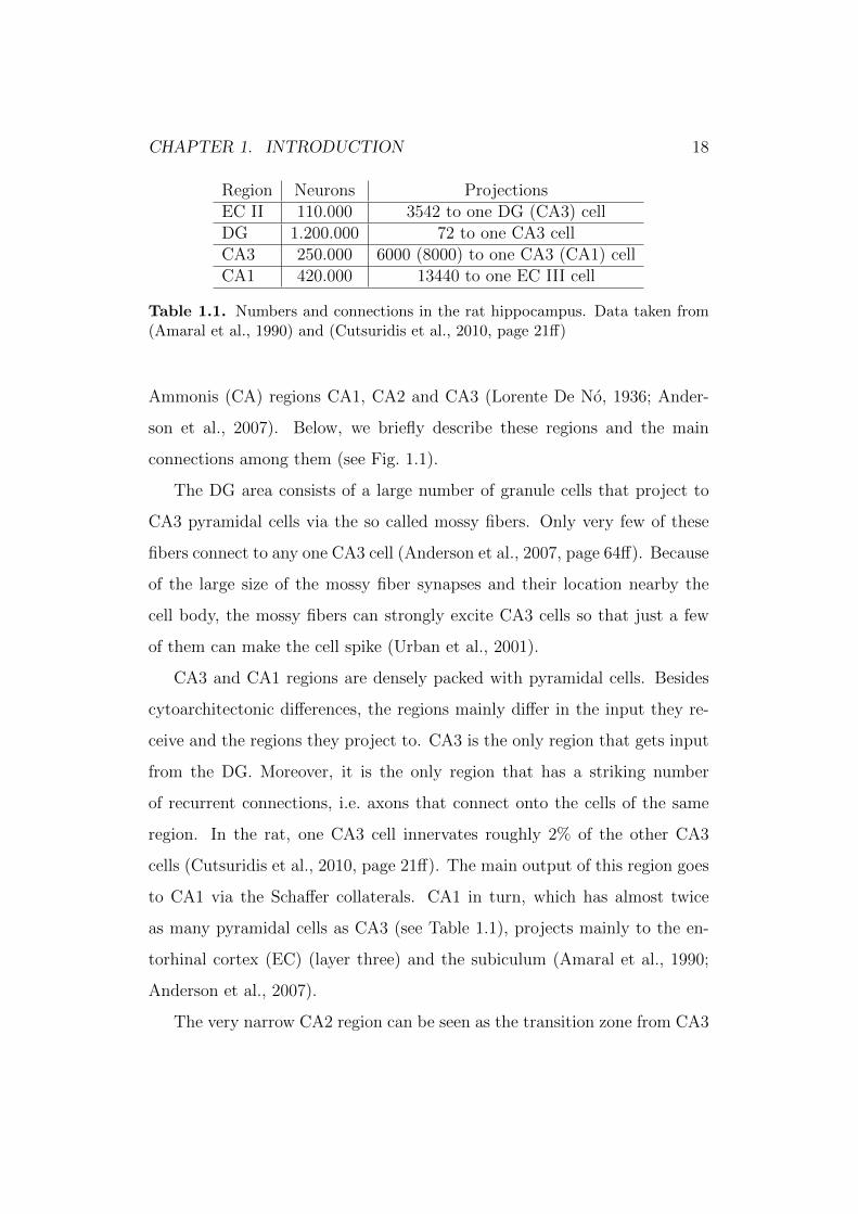
Region Neurons ProjectionsEC II 110.000 3542 to one DG (CA3) cellDG 1.200.000 72 to one CA3 cellCA3 250.000 6000 (8000) to one CA3 (CA1) cellCA1 420.000 13440 to one EC III cell
Table 1.1. Numbers and connections in the rat hippocampus. Data taken from(Amaral et al., 1990) and (Cutsuridis et al., 2010, page 21ff)
Ammonis (CA) regions CA1, CA2 and CA3 (Lorente De No, 1936; Ander-
son et al., 2007). Below, we briefly describe these regions and the main
connections among them (see Fig. 1.1).
The DG area consists of a large number of granule cells that project to
CA3 pyramidal cells via the so called mossy fibers. Only very few of these
fibers connect to any one CA3 cell (Anderson et al., 2007, page 64ff). Because
of the large size of the mossy fiber synapses and their location nearby the
cell body, the mossy fibers can strongly excite CA3 cells so that just a few
of them can make the cell spike (Urban et al., 2001).
CA3 and CA1 regions are densely packed with pyramidal cells. Besides
cytoarchitectonic differences, the regions mainly differ in the input they re-
ceive and the regions they project to. CA3 is the only region that gets input
from the DG. Moreover, it is the only region that has a striking number
of recurrent connections, i.e. axons that connect onto the cells of the same
region. In the rat, one CA3 cell innervates roughly 2% of the other CA3
cells (Cutsuridis et al., 2010, page 21ff). The main output of this region goes
to CA1 via the Schaffer collaterals. CA1 in turn, which has almost twice
as many pyramidal cells as CA3 (see Table 1.1), projects mainly to the en-
torhinal cortex (EC) (layer three) and the subiculum (Amaral et al., 1990;
Anderson et al., 2007).
The very narrow CA2 region can be seen as the transition zone from CA3

CHAPTER 1. INTRODUCTION 19
MEC
LEC
LEC
MEC
Figure 1.1. The two pathways through the hippocampus. Illustration ofthe main connections in the hippocampal formation. A: The trisynaptic pathwayEC-DG-CA3-CA1-EC pathway. B: The temporoammonic pathway EC-CA1-EC.

CHAPTER 1. INTRODUCTION 20
to CA1 and its existence has often been questioned (Anderson et al., 2007,
p.43). CA2 pyramidal cell bodies are the same as the ones in CA3, but like
CA1 cells they do not receive mossy fiber input from the DG.
The main input structure of the hippocampus is the EC, which itself can
be divided into the medial entorhinal cortex (MEC) and the lateral entorhinal
cortex (LEC). Neurons in layer two of both parts project to the DG and to
CA3. Neurons of layer three of the EC project to CA1, where the proximal
CA1 side (the side near CA3) receives more input from the medial part
and the distal side (near the subiculum) receives more input from the LEC
(Igarashi et al., 2014).
In conclusion, the information flow across the hippocampus is mainly
unidirectional and follows two main pathways: The so called trisynaptic
pathway EC-DG-CA3-CA1-EC and the temporoammonic pathway EC-CA1-
EC.
1.2 Hippocampal memory function
1.2.1 Crucial role in memory formation
The crucial role of the hippocampus in memory formation is well known. The
most prominent evidence is the case study of patient H.M. whose hippocampi
and nearby cortices had been removed. After surgery he had severe deficits in
acquiring new episodic memory (anterograde amnesia) and in remembering
events that happened shortly before the damage (retrograde amnesia) (Mil-
ner et al., 1968; Corkin, 2002). Older memories, however, have been spared
from the lesions. This lead to the theory of systems consolidation (Squire and
Alvarez, 1995; Frankland and Bontempi, 2005). Based on this theory new
declarative memories (episodic and semantic memories) are initially encoded

CHAPTER 1. INTRODUCTION 21
in the hippocampus and then slowly transferred to the neocortex where it
is permanently stored. As a result, memories become independent of the
hippocampus after some time. Further research have shown that stabilized
memories can become hippocampus dependent again, once the memory has
been retrieved again, which lead to the theory of re-consolidation (Nader
et al., 2000). Interestingly, additional studies on patient H.M. showed that
many other of his cognitive abilities including some other memory functions
remained intact. For example, the retention of information for short time
intervals or the acquisition of new procedural memories (learning new mo-
tor skills) were unaffected (Corkin, 2002). Neuropsychological analysis on
amnesic patients and functional imaging studies further confirm the impor-
tance of the hippocampus in establishing new episodic memories in humans
(Burgess et al., 2002).
Impairments in memory formation can be observed in animals, too (Squire
et al., 2004). A large body of studies in rodents show that the hippocampus
supports spatial memories, i.e. memories of locations in relation to external
landmarks, which lead to the theory that the hippocampus builds an inter-
nal ’cognitive map’ of space (OKeefe and Nadel, 1978; McNaughton et al.,
2006). Other work show that the hippocampus is also involved in non-spatial
memories (see for example (Eichenbaum et al., 1999). For instance, rats with
a lesioned hippocampus cannot associate stimuli if there is a time delay be-
tween them (Gluck and Myers, 2001).

CHAPTER 1. INTRODUCTION 22
1.2.2 The standard model of memory formation
Pattern completion in CA3
The question that arises from the previous sections is, how does the peculiar
anatomical structure of the hippocampus serve memory formation? Over the
years, a standard model has been developed regarding hippocampal function
and it has been tested with a number of computational models (for example
by Rolls (1995); Weisz and Argibay (2009)). A memory or episodic event is
typically interpreted as an activation pattern of a set of neurons in the input
structure of the hippocampus. Once a memory is stored in the hippocampal
network, recall is modelled by initializing the network with a partial recall
cue, i.e. a corrupted or incomplete version of this memory and retrieval is
considered successful, if the whole pattern could be reconstructed. This
process is called pattern completion.
The main idea of the standard model is that pattern completion is per-
formed by an auto-associative memory or attractor network (Marr, 1971;
McNaughton and Morris, 1987; Treves and Rolls, 1994; O’Reilly and Mc-
Clelland, 1994; Rolls, 2007). An attractor network is a recurrent network
equipped with so called attractor states, which are certain patterns of neural
activation imprinted on its connections. Once initialized randomly, the acti-
vation pattern in the network will converge over time towards one of those
patterns and will remain in this state.
Given the anatomical requirements it has been suggested that CA3 func-
tions as such a network. It stores patterns in its recurrent connections by
using an auto-associative learning rule. In this way each stored pattern be-
comes an attractor state in the network’s dynamics (see (Amit, 1989)). Dur-
ing recall a partial cue is then attracted towards the originally stored pattern

CHAPTER 1. INTRODUCTION 23
and hence the pattern is completed as soon as the network has settled down
on the attractor. Thus, the actual storing place are the recurrent connections
and this idea explains why there are so remarkably many in CA3.
Pattern Separation in DG
An auto-associative memory can only store patterns that are not similar
or mutually correlated (Marr, 1971; Amit, 1989; Rolls, 2007). By nature,
however, the neural activation in the input region of the hippocampus, the
EC, is not uncorrelated (Hafting et al., 2005). Thus, it has been suggested
that the DG performs the so called pattern separation during the storage
phase (McNaughton and Morris, 1987; Treves and Rolls, 1994; O’Reilly and
McClelland, 1994; Rolls, 2007). It decorrelates the patterns of the EC and
projects the separated versions of the patterns to CA3 for storage. A large
number of cells with low activity and the sparse projections of mossy fibers
support pattern separation computationally (Rolls, 2007; Treves et al., 2008).
Hence, this view explains the appearance of further prominent hippocampal
characteristics. Finally, it has been proposed that the role of CA1 is to decode
the highly transformed patterns in CA3 back to their original versions in the
EC.
Since the introduction of the model, the computational functions of pat-
tern completion and pattern separation have been highly discussed. Experi-
mental studies have not only tried to find direct evidence for these operations
through neuronal recordings (see for example (Guzowski et al., 2004; Leut-
geb et al., 2007; Bakker et al., 2008), but have also reinterpreted them on a
behavioural level (see for a review (Kesner et al., 2004; Santoro, 2013)).

CHAPTER 1. INTRODUCTION 24
1.3 Spatial representations in the hippocam-
pal formation
Besides its outstanding anatomy and its function in memory formation, the
hippocampus is famous for having cells that are receptive to certain locations
in space. Electrophysiological recordings have also revealed that cells in the
hippocampal formation not only respond to locations but also to other high
level ’stimuli’. In what follows we briefly describe the different cell types in
the hippocampal formation of rodents categorized based on their preferred
stimulus.
1.3.1 Place cells in the hippocampus
Probably the most prominent cell type in the hippocampus is the place cell.
It is highly active when the animal is at a well defined region in the environ-
ment called place field and fires typically at low rate elsewhere (O’Keefe and
Dostrovsky, 1971; Moser et al., 2008). Place cells have been found through-
out all subregions in the hippocampus (O’Keefe, 1979; Leutgeb et al., 2005a,
2007) and are likely to be pyramidal cells in the CA regions (Henze et al.,
2000) and granule cells in the DG (Jung and McNaughton, 1993; Leutgeb
et al., 2007).
Place cells in the CA regions typically have one or two place fields,
whereas in the DG cells tend to have more but smaller fields (Jung and
McNaughton, 1993; Leutgeb et al., 2007). Cells have their place fields at
different locations such that across the population the entire physical space
is covered and the location of the animal can be reconstructed accurately
by monitoring the firing rates of a small set of place cells (Wilson and Mc-
Naughton, 1993; Zhang et al., 1998).
CHAPTER 1. INTRODUCTION 25
Field sizes express a fair amount of variance within animals (Mizuseki
et al., 2012), but the average place field size increases from dorsal sites to
ventral sites (Jung et al., 1994; Maurer et al., 2005; Kjelstrup et al., 2008) of
the hippocampus.
Almost all pyramidal cells can exhibit place fields, but only a fraction
of them do so in any given environment (see Table 2.1 in Methods). Ap-
parently, there is no relationship between the subset of cells that are active
and locations of their place fields across environments (O’Keefe and Conway,
1978; Thompson and Best, 1989; Alme et al., 2014).
The location of place fields can be very stable between different visits in
the same environment (Thompson and Best, 1990; Moser et al., 2008). They
can also be remarkably robust against the removal of some environmental
cues (O’Keefe and Conway, 1978; Moser et al., 2008). However, due to
some changes to the environment they can alter their firing rates, a process
called rate remapping (Anderson and Jeffery, 2003; Leutgeb et al., 2005a).
Moreover, due to larger manipulations of the environment an entire new set
of active cells can be recruited and cells active in both environments can
change their firing location. This phenomenon is called global remapping
(Bostock et al., 1991; Leutgeb et al., 2004; Alme et al., 2014).
1.3.2 Grid cells in the MEC
Contrary to hippocampal place cells grid cells in the medial entorhinal cortex
have several place fields highly ordered on a hexagonal grid (Fyhn et al., 2004;
Hafting et al., 2005). This grid pattern can be described by three properties:
its orientation, its spatial phase and its grid spacing (Fig. 1.2).
The grid orientation is the orientation of the grid axes relative to some
reference direction and is by definition between 0 and 60 degrees. The spa-

CHAPTER 1. INTRODUCTION 26
Figure 1.2. Parameters of a grid cell. When the firing rates of a cell areplotted over space, one gets the so called rate map of the cell. The figure showsthe rate map of a modelled grid cell in a 2 m by 1 m rectangular environment.Red indicates high firing rates and blue low firing rates. One can define a gridcell by three parameters: the grid orientation θ (relative to an arbitrarily defineddirection), the spacing between two vertices s, and the spatial offset or phase (x, y).
tial phase specifies the spatial offset of the grid pattern with respect to a
reference point. Finally, the spacing is defined as the distance between two
neighbouring vertices on the hexagonal grid (on a hexagonal grid this dis-
tance is constant among all pairs of neighbouring vertices). The sizes of the
place fields that are located at the grid vertices scale proportionally with the
cell’s grid spacing (Hafting et al., 2005, Fig.S4G).
Initially, it has been thought that grid spacings increase continuously
from dorsomedial to ventrolateral locations of the MEC (Hafting et al., 2005)
mirroring the increase of size of place fields along the dorsoventral axis in the
hippocampus. Recent findings, however, suggest that grid cells are organized
in discrete modules with similar spacings and orientations and that modules
with small spacings are predominantly in dorsal regions and modules with
large spacings in more ventral entorhinal areas (Barry et al., 2007; Stensola
et al., 2012). The spatial phase appears to be uniformly distributed in all
modules and a topography has not been found yet (Moser et al., 2008, 2014).

CHAPTER 1. INTRODUCTION 27
Like place cells, grids cell patterns are remarkably stable during repeated
exposure to the same environment (Hafting et al., 2005). Moreover, when
exposed to a novel environment grid patterns remap. The offsets shift ran-
domly and the patterns rotate by random amounts, whereby cells recorded
at the same location rotate coherently (Fyhn et al., 2007). The spacings of
the cells are constant across environments, however, during the first days of
exposure they are larger (Barry et al., 2012). Interestingly, this remapping
appears to occur exactly, whenever global remapping in the hippocampus is
observed (Fyhn et al., 2007; Barry et al., 2012).
1.3.3 Other cell types in the MEC
Besides grid cells a few other cell types have been found in the MEC. Two
prominent examples are head direction cells and border cells.
A head direction cell has a preferred direction, i.e. it fires only rapidly
when the animal’s head is pointing into this direction independently of the
current location of the animal (Taube et al., 1990a,b; Sargolini et al., 2006).
Across the MEC population a full range of directions is presented and it is
possible to reconstruct the animals head direction accurately just by moni-
toring the firing rates of a small number of head direction cells (Zhang, 1996;
Johnson et al., 2005)
Border cells, also known as boundary cells, are active whenever a bound-
ary is at a particular distance and direction from the animals location (Sol-
stad et al., 2008; Savelli et al., 2008) independently of head direction. When
a second boundary is inserted to the environment they express a further place
field at the same distance and direction to the new boundary.
Head direction cells and border cells, as well as grid cells maintain their
firing behaviour in darkness (Taube et al., 1990a; Hafting et al., 2005; Lever

CHAPTER 1. INTRODUCTION 28
et al., 2009) and rotate coherently when polarising visual stimuli are moved
(Knierim et al., 1995; Hafting et al., 2005; Sargolini et al., 2006; Solstad et al.,
2008). This suggest that these cell types are coupled to sensory input and
that they are influenced by self-motion cues.
Additionally, many spatially and non-spatially selective cells are observed
in the MEC that do not fit into the three categories above (Krupic et al.,
2012; Zhang et al., 2013). Roughly estimated, around 30% of MEC cells are
grid cells, 20% are head direction cells and less than 10% are border cells
(Solstad et al., 2008; Krupic et al., 2012; Zhang et al., 2013).
1.3.4 Cells in the LEC
In contrast to the MEC, cells in the LEC express only little spatial selectivity
and carry much weaker self-motion information (Neunuebel et al., 2013).
Recordings have shown that single LEC cells in the rat are receptive to
individual items such as odours (Young et al., 1997) or objects (Zhu et al.,
1995b,a; Deshmukh and Knierim, 2011). In the monkey they respond to
pictures of objects and their location on the monitor (Suzuki et al., 1997).
Thus, when a rat explores an environment with only few objects, cells
carry much less spatial information compared to the MEC and rate maps
are less stable between visits to the same environment (Hargreaves et al.,
2005). This is also true in environments containing many spatial landmarks
(Yoganarasimha et al., 2011). Nevertheless, the LEC signal still carries some
amount of spatial information (Neunuebel et al., 2013).
In environments that are enriched with some objects, spatial information
reaches the level of grid cells (Deshmukh and Knierim, 2011). Here, addi-
tional to cells receptive to individual objects, a small number of cells fire like
hippocampal place cells at regions where the animal had never experienced

CHAPTER 1. INTRODUCTION 29
an object. Other cells fire at locations where an object has been removed
and this memory response can last for days to weeks (Tsao et al., 2013).
1.4 From grid cells to place cells
1.4.1 Grid cells may be responsible for place cell firing
Both grid cells and place cells are similarly dependent on landmarks and
boundaries of the environment. They exhibit stable firing pattern during
repeated visits of the same environment (Thompson and Best, 1990; Mc-
Naughton et al., 2006), are robust to the removal of some environmental
cues (O’Keefe and Conway, 1978; Hafting et al., 2005), mostly preserve their
firing maps in darkness (Quirk et al., 1990; Zhang et al., 2014), rotate their
spatial firing maps in concert with the displaced landmark (Muller and Ku-
bie, 1987; Hafting et al., 2005), rescale the size of the place fields when the
environment is expanded (O’Keefe and Burgess, 1996; Barry et al., 2007) or
becomes familiar to the animal (Mehta et al., 1997; Lee et al., 2004a; Barry
et al., 2012), and their representation remap simultaneously (Fyhn et al.,
2007; Barry et al., 2012). Moreover, the field sizes of both cell types increase
along the dorsoventral axis (Fyhn et al., 2007; Kjelstrup et al., 2008), con-
sistent with topographic projections from EC to the hippocampus along the
same axis (Dolorfo and Amaral, 1998; Honda et al., 2012).
Because of these similarities and since grid cells are found just one synapse
upstream from place cells, it has been suggested by many scientists that the
former is responsible for the activation of the latter (for example (Fuhs and
Touretzky, 2006; McNaughton et al., 2006; Rolls et al., 2006; Solstad et al.,
2006; Blair et al., 2007; Franzius et al., 2007), but see (Moser et al., 2008)).
However, some experimental evidence has accumulated that place cells

CHAPTER 1. INTRODUCTION 30
Study Field Size Number Reference
Model (ICA) very small ≈ 1 Franzius et al. (2007)Model (competitive learning) 350cm2 1.2 Si and Treves (2009)Model (competitive activation) 627cm2 1.5 de Almeida et al. (2009)Model (random weights; CA3) 290cm2 1.1 de Almeida et al. (2012)Model (predefined weights) < 420cm2 1 Azizi et al. (2014)
Measurement DG < 900cm2 3-4 personal communicationwith Edvard Moser
Measurement CA3 1275cm2 1.5 Mizuseki et al. (2012)Measurement CA1 1725cm2 1.4 Mizuseki et al. (2012)
Table 1.2. Comparison of place field sizes and numbers in selected studies
emerge without the drive of grid cells (Wills et al., 2010; Langston et al.,
2010; Koenig et al., 2011; Brandon et al., 2011) and other suggestions of
place cell formation exists. For example some authors propose that place
cells are the product of border cells (Hartley et al., 2000; Burgess et al., 2000)
or others even argue vice versa that place cells trigger grid cells (Castro and
Aguiar, 2014).
1.4.2 Grid-to-place transformation
Quite a few theoretical models have shown that it is possible to create a place
cell population out of the activation of grid cells in a simple feedforward
network by competitive learning (Rolls et al., 2006; Si and Treves, 2009),
through competitive cell activation (de Almeida et al., 2009), by a Fourier
transformation (Solstad et al., 2006), by defining weights in a specific manner
(Azizi et al., 2014), by Hebbian learning (Savelli and Knierim, 2010), by
independent component analysis (Franzius et al., 2007) or by applying linear
regression (Blair et al., 2007). However, all these methods either produce
place fields of limited size (see Table 1.2) or, in the case of linear regression,
are highly sensitive to noise (Cheng and Frank, 2011).

CHAPTER 1. INTRODUCTION 31
The average place field size in the noise robust models roughly corre-
sponds to the small place field size of granule cells in the rat dentate gyrus.
However, in the CA-regions place fields are significantly larger (Mizuseki
et al., 2012) and to the best of our knowledge there are no ’grid to place’
models that reproduce robust fields of these sizes.
1.5 Content of the thesis
The goal of this thesis is to present a unifying computational model that
accounts for both, hippocampal memory function and the formation of spatial
representations in the hippocampus.
The prominent standard model described in Section 1.2.2 explains only
memory formation but ignores the appearance of hippocampal spatial rep-
resentations. In Chapter 3 we review the standard model and we reveal
computational inefficiencies. In particular, when neural patterns in the EC
resemble more realistic grid cell activity instead of random activity, an auto-
associative CA3 network is harmful for memory performance. This is in
contradiction to the ideas of the standard model and challenges it seriously.
Therefore we propose an alternative model that patterns are stored in the
feedforward connections of the temporoammonic pathway EC-CA1-EC and
we show that this model is indeed more efficient in pattern completion.
In Chapter 4 we focus on the formation of hippocampal spatial represen-
tations. Many models argue that place cells are triggered by grid cells in a
feedforward network. We study the general structure of such a network that
all models have in common and we show that it is not plausible that a simple
feedforward model creates robust place fields of realistic size as found in the
CA regions of rodents. As an alternative model we propose that place cells

CHAPTER 1. INTRODUCTION 32
are mainly triggered by other entorhinal cell types that are weakly spatially
modulated. We test this hypothesis on the EC-CA1-EC model, which we
introduced in Chapter 3. We found that the model can produce large and
robust place fields. Moreover, it reproduces many other place cells charac-
teristics as well as results from studies in lesioned animals and makes some
strong predictions.
Thus, we present a simple model that outperforms the more complex stan-
dard model in memory formation. At the same time this model reproduces
hippocampal place cell characteristics and overcomes the issue of creating
robust place fields of realistic size.
In Chapter 2 we describe the methods we use. In particular, the model
is described in detail there. Finally, we discuss our results in Chapter 4.

Chapter 2
Methods
2.1 The standard model
2.1.1 Model architecture and activation function
The model consists of the regions EC, DG, CA3 and CA1. Cell numbers
NEC , NDG, NCA3 and NCA1 in each region and numbers of connections one
cell in a downstream region receives from an upper region are summarized in
Fig 2.1. Cell numbers and numbers of connections are derived from rat data
(Amaral et al., 1990; Cutsuridis et al., 2010, and see Table 1.1) and scaled
down by 100 and 10, respectively. Dividing the number of connections per
cell by 100, too, would lead to CA3 cells that do not receive any input from
the DG. On the other hand, leaving this number constant would result in
triple connections among cell pairs in the network. Thus, we choose to scale
by a value between the two extremes. Cells in our model have continuous
firing rates with the exception of CA3 cells, which are binary, i.e., they either
fire and have the value 1 or are silent and have the value 0. This is in line
with Rolls (1995), where CA3 does not work well with continuous firing rates
33

CHAPTER 2. METHODS 34
EC
N=1100; a=0.35
CA3
N=2500;a=0.032
DG
N=12000; a=0.0078
Figure 2.1. The standard model. The four subregions EC, DG, CA3 andCA1 are modelled. a denotes the proportion of cells being active at any giventime. Arrows indicate connectivity among regions. Black ones are random andfixed connections, green ones are plastic and adjusted during learning. The numbernext to the arrows show the number of connections one cell in the downstreamregion has with the up stream region.
(Rolls, 1995).
A pattern p of neural activation, for example, p ∈ RNEC+ in the EC triggers
neural activity in a downstream region, e.g., in the DG, via the connections
as follows: First, the activation hi of the output cell i is calculated by the
standard weighted sum of its inputs
hi =N∑j=1
wijpj, (2.1)
where wij is the strength of the connection from cell j to cell i and is defined
as 0 whenever this connection is not existent.
To determine the firing of a cell a simple k-Winner-Take-All (kWTA)
mechanism is applied: After calculating the activation of all cells of that

CHAPTER 2. METHODS 35
region, the k cells with the highest activation are either set to 1 or to hi
whenever they are continuous. The others are inhibited and set to 0. The
number k is determined by the sparsity a of that region, i.e k = aN . For
instance, the pattern of neural activity q ∈ RNDG+ in the DG is
qi =
hi if hi is among the k highest {hj : 1 ≤ j ≤ NDG}
0 otherwise.(2.2)
Thus, inhibitory cells are not modelled explicitly but rather through their
effect on a population level (Roudi and Treves, 2008; Moustafa et al., 2009;
Renno-Costa et al., 2010; Appleby et al., 2011; Monaco and Abbott, 2011).
In order to determine the sparsity a in one region (the proportion of
cells being active at each location) we multiply the average proportion of
cells being active in the entire environment by the average proportion of the
environment a cell is typically active in. We have estimated the average
proportion of cells being active in the entire environment by referring to
several studies that count active cells by immediate early genes (Vazdarjanova
and Guzowski, 2004; Alme et al., 2010; Marrone et al., 2011; Satvat et al.,
2011) or by electrophysiological recordings (Leutgeb et al., 2004; Lee et al.,
2004b). Individual reports are summarized in Table 2.1 and yield average
activity levels of 2.9% in the DG, 22.7% in CA3 and 42.7% in CA1 across the
enclosure. To estimate the average proportion of the environment a cell is
active in we use data from recordings within a 1m2 apparatus (Leutgeb et al.,
2004, Supplementary Table 1) and we obtain a coverage of 14% of a CA3 cell,
and 21% of a CA1 cell. A typical DG cell has 3-4 fields and a field size smaller
than 900cm2 (personal communication with Edvard Moser) which brings us
to an estimation of 27% coverage. Multiplying the proportion of cells being
active across the environment by the proportion of the environment one active

CHAPTER 2. METHODS 36
Study Method Active cells %DGSatvat et al. (2011) (Fig. 3) IEG 3Marrone et al. (2011) (Fig. 5) IEG 3-4Alme et al. (2010) (Fig. 7) IEG 2.2CA3Vazdarjanova and Guzowski (2004) (Fig.3c) IEG (Arc, Homer1) 18Leutgeb et al. (2004) Electrophysiology 17-32Lee et al. (2004b) Electrophysiology 26CA1Vazdarjanova and Guzowski (2004) (Fig.3c) IEG (Arc, Homer1) 35Leutgeb et al. (2004) Electrophysiology 48-66Lee et al. (2004b) Electrophysiology 36
Table 2.1. Overview of measured activity levels in hippocampal subre-gions. The table shows an overview of selected studies which measure the activitylevels in hippocampal subregions either by electrophysiological recordings or by im-mediate early genes (IEG). Last column shows percentage of cells active in oneenvironment.
cells fires leads to the activation level at one location given by a (see Fig 2.1).
For the EC we calculated the average coverage of a grid cell to be 35% using
data from Hafting et al. (2005) and assume that a grid cell is active in every
environment (Hafting et al., 2005; Fyhn et al., 2007). This value is similar
to the estimation made by other authors publishing a computational model
(de Almeida et al., 2009).
2.1.2 Learning rules
To store patterns in the network the plastic weights among subregions (green
arrows in Fig 2.1) are adjusted by three related Hebbian learning rules. Let
C denote the connection matrix of two regions, i.e., cij = 1 if there is a
connection from cell j to i and cij = 0 otherwise.
For the connections EC to CA3, CA3 to CA1, and CA1 to EC a rule for
hetero-association is used. Let {p(s) : 1 ≤ s ≤ M} be the set of M input

CHAPTER 2. METHODS 37
patterns and {q(s) : 1 ≤ s ≤ M} be the set of output patterns, then the
connection strength is defined according to the so called Stent-Stinger rule
(Stent, 1973)
wij = cij
M∑s=1
(p(s)j − pj)q
(s)i , (2.3)
where the connection from cell j to i is the sum over all patterns s of firing
p(s)j of input cell j subtracted by its mean pj times the firing q
(s)i of cell i.
The factor cij assures that non-existing connections remain at zero weight.
For the synaptic weight matrix V of the recurrent weights in CA3 the
co-variance rule is used (Sejnowski, 1977) to learn an auto-association among
a set of patterns {p(s) : 1 ≤ s ≤M}
vij = cij
M∑s=1
(p(s)j − pj)(p
(s)i − pi). (2.4)
By subtracting the mean the two learning rules model LTP and LTD. Fur-
thermore the subtraction is essential for computational reasons (see for ex-
ample (Amit, 1989, chapter 8.2)).
Finally, the connections from EC to DG are altered by a one shot com-
petitive learning rule. Here, the current input pattern p first triggers a
firing pattern q in the downstream region according to the equations above.
Synapses are then changed by
wij = cij(woldij + γpjqi), (2.5)
where γ is a constant learning rate. After applying equation (2.5) the Eu-
clidean norm of vector wi of incoming weights to cell i is normalized to one to
assure that not always the same cells get activated. These rules are adopted

CHAPTER 2. METHODS 38
from Rolls (1995) to keep the model as similar as possible to that one.
After hetero-association of {p(s) : 1 ≤ s ≤ M} with {q(s) : 1 ≤ s ≤ M}
by applying equation (2.3) between some regions, given pattern p(t) as the
present input we can rewrite the activation h(t)i as
h(t)i
(2.1)=
N∑j=1
wij p(t)j (2.6)
(2.3)=
N∑j=1
cij
M∑s=1
(p(s)j − pj)q
(s)i p
(t)j (2.7)
= q(t)i
N∑j=1
cij(p(t)j − pj) p
(t)j +
∑s 6=t
q(s)i
N∑j=1
cij(p(s)j − pj) p
(t)j (2.8)
≈ q(t)i c (p(t) − p)Tp(t)︸ ︷︷ ︸St
+∑s 6=t
c q(s)i (p(s) − p)Tp(t)︸ ︷︷ ︸
X(i,s,t)
, (2.9)
where c is the proportion of cells one output cell is connected to in the input
layer. Thus, we can write the activation of cell i as the sum of a signal term
q(t)i St which comes from the weights arising from the storage of pattern p(t)
and the crosstalk terms X(i,s,t) which come from the contribution of the other
stored patterns in which this cell was active (Willshaw and Dayan, 1990)
h(t)i ≈ q
(t)i St +
∑s 6=t
X(i,s,t). (2.10)
Ideally, the activation is high if and only if the cell has fired in pattern q(t).
2.1.3 Storage and recall
Storing a pattern p of entorhinal activation in the network is done as follows.
First, this pattern triggers neural activity in the DG which in turn triggers
a pattern in the CA3 region via equations (2.1) and (2.2). Thus, during

CHAPTER 2. METHODS 39
storage, activity in CA3 is only influenced by the mossy fiber input from the
DG. The connections from EC to DG are altered by the competitive learning
rule (equation (2.5)) for pattern separation. Hence, for the next pattern the
connections are different than for the current pattern. Furthermore, p drives
an activity pattern in CA1. Now, the pattern in CA3 is hetero-associated
with p in EC, auto-associated in the recurrent connections in CA3, and
hetero-associated with the pattern in CA1. Finally, the CA1 activity is
hetero-associated with p in the EC.
After the storage of all patterns the network is presented a recall cue by
setting entorhinal activity to a noisy version p of a previously stored pat-
tern. This activity triggers a pattern q(0) in CA3 directly via the previously
learned weights from EC to CA3. The pattern then runs through 15 acti-
vation cycles of the auto-associative network in CA3 while leaving the input
from EC clamped1. In more detail, for the t-th cycle the activation of CA3
cell i is
hi(t) = α
NEC∑j=1
wEC−CA3ij pj + β
NCA3∑j=1
vij qj(t− 1), (2.11)
where α and β are constant factors set to 1 and 3 and q(t) is determined by
the k-WTA mechanism described in equation 2.2. Hence, during recall CA3
activity is dominated by the recurrent connections and the DG is not involved
anymore. The resulting pattern q(15) triggers a pattern in CA1, which in
turn determines the output pattern in the EC via the learned weights from
CA3 to CA1 and CA1 to EC, respectively.
1we have verified that after 15 cycles the results have converged.

CHAPTER 2. METHODS 40
2.2 Alternative models
2.2.1 Standard model without CA3 recurrence
In Chapter 3 we compare the recall ability of the standard model to the abil-
ity of two alternatives. Firstly, to determine how effective the CA3 recurrent
connections are, we perform simulations of a network without these connec-
tions (Fig. 2.2A). Here, the pattern q(0) defined in Section 2.1.3 is directly
transferred to CA1 during recall without undergoing the activation cycles
of the auto-associative network in CA3. The result of these simulations are
indicated by dashed lines throughout the figures in Chapter 3.
2.2.2 EC-CA1-EC model
Secondly, we investigate the ability of a minimal EC-CA1-EC model to store
patterns (Fig. 2.2B). In this model, during storage, activity in CA1 is trig-
gered by input from the EC-CA3-CA1 pathway, without any plasticity in
these connections. The CA1 patterns are then hetero-associated with the
original input patterns in the connection weights EC-CA1 and CA1-EC, so
in contrast to previous models the EC-CA1 connections are now plastic.
During the recall phase the recall cue is transferred to CA1 via the tem-
poroammonic pathway (EC-CA1) and from there back to EC. The result of
these simulations are indicated by magenta lines throughout the figures in
Chapter 3.
Since it will come out that this simpler model performs best, we further
investigate its ability of creating robust and realistic sized place fields in
Chapter 4.
Besides the architecture outlined above, parameters do not change across
simulations except in section ’Comparison to the Model in Rolls (1995)’. All

CHAPTER 2. METHODS 41
plastic
xed
A
EC
CA3
DG
Figure 2.2. Alternative models. A: The standard model without recurrentconnections in CA3. Here, patterns are stored only in the remaining plastic feed-forward connections (in green). B: The EC-CA1-EC model. Only the connectionsfrom EC to CA1 and from CA1 to EC are plastic. During storage CA1 patternsare triggered by CA3. During recall the cue in EC is projected to CA1 directlyvia the EC-CA1 connections and is then reconstructed in EC via the CA1-ECconnections.

CHAPTER 2. METHODS 42
parameter changes there are described in the main text.
2.3 General feedforward model
In Chapter 4 we study an additional generic model to investigate whether
it is possible to generate realistic place fields in a feedforward network, in
principle, based solely on grid cell input (Fig. 2.3). The network consists of
an input layer containing grid cells and an output layer containing purported
place cells. We denote the population vector (PV) of grid cell activity at
location r as p(r). Each output cell i is activated by grid cell inputs weighted
by the vector wi.
hi(r) = wTi p(r) (2.12)
To determine when the output cell fires spikes, a monotonic activation func-
tion f(hi) is applied. Suppose cell i has a place field at location ri with radius
Ri. If we want the neuron to fire spikes inside the field and not elsewhere,
then the activation hi(r) must be higher within the field than outside it, since
the activation function f is monotonic. Hence, there must be some threshold
c such that
wTi p(r) ≥ c ∀r : ||r− ri|| ≤ Ri
∧ wTi p(r) < c ∀r : ||r− ri|| > Ri. (2.13)
Up to here, the model is general and subsumes several previous models
(Rolls et al., 2006; Solstad et al., 2006; Blair et al., 2007; Si and Treves, 2009;
de Almeida et al., 2009; Savelli and Knierim, 2010; Azizi et al., 2014). Specific
models differ only in the activation function and in the way the weights are
set up.

CHAPTER 2. METHODS 43
. . .p1 p2 p3 pN
w2 w3 wNw1
f(wTp)
A B
p
Figure 2.3. General feedforward model.. A: Magenta arrow illustrates apopulation vector p at some location. The components of the vector are the firingrates of the cells at that location. B: Sketch of the general model. At each locationthe firing of the downstream cell is determined by a monotonic function f of thesum the grid cell inputs p weighted by connections weights w. Ideally, this resultsin a place field.
2.3.1 Linear classification
We can regard the problem of finding the weight vector and threshold ful-
filling Eq. 2.13 as a linear classification problem. A putative weight vector
defines a hyperplane in the input space and classifies the PVs into two classes
depending on which side of the plane the PV is located (see Fig. 2.4). An
optimal weight vector, which fulfils Eq. 2.13, splits the input space such that
on one side are all PVs referring to locations within the place field and on
the other side are all PVs located outside the place field.
Linear classification is well studied and there are some established ma-
chine learning algorithms. We apply a linear support vector machine to find
the weight vector and threshold for circular place fields with a radius of 10cm,
25cm and 35cm. This classifier does not only find a solution when it exists,
but also returns the solution that is most robust, in the sense that the dis-
tance from the nearest PVs to the hyperplane is maximal (see for example
(Hastie et al., 2009, chapter 4.5.2)).

CHAPTER 2. METHODS 44
wri
ng r
ate
cell 1
ring rate cell 2
Figure 2.4. Linear classification. Cartoon that shows 40 PVs of a populationof two neurons. Colours indicate whether the location of the PV is inside a givenplace field or outside the place field. In this example the vector w is able toseparate the two classes perfectly.
Additionally, to make sure the results obtained by the linear support
vector machine are not dependent on the choice of the algorithm, we apply
two more linear classification algorithms for the largest place field size: Linear
and logistic regression. For all algorithms we use the implementation of the
python package sklearn (Pedregosa et al., 2011). We refer the reader to
(Hastie et al., 2009, chapter 4)) for detailed information about the algorithms.
2.4 Input
For the study of memory formation in Chapter 3 we investigate the storage
of three different kinds of patterns in the EC. Patterns made of randomly
firing cells, patterns made of grid cells and patterns made of a mixture of
grid cells and weakly spatially modulated cells. To do so we build a 1m by
1m virtual square environment discretized into 400 locations. For every cell a

CHAPTER 2. METHODS 45
rate map is defined which determines the cell’s firing rate at each location in
the environment. After the rate maps have been created as described below,
252 locations are drawn randomly. At each of them firing rates of all cells
but the k ones with the highest activation are set to zero as in equation (2.2)
to control for sparsity. The resulting PV is considered a pattern for storage.
In the study of place cell formation in Chapter 4 patterns are made of
grid cells and of a mixture of grid cells and weakly spatially modulated cells.
Here, a 2m by 1m virtual environment is created and discretized into 2.5 x
2.5cm2 bins (3200 locations) to match the methods in (Stensola et al., 2012)
closely. Controlling for sparsity is not necessary and a kWTA mechanism is
not applied to the input.
2.4.1 Randomly firing cells
At every location cell activity hi of a randomly firing cell is sampled from a
normal distribution with mean and variance equal to 1.
2.4.2 Grid cells
We model the grid cell population closely to data recorded in (Stensola et al.,
2012). This data is obtained from recordings in the dorsal MEC covering up
to 50% of the dorsoventral axis. Thus, we model the input to a typical
dorsal cell in the hippocampus, since the projections to the hippocampus
are topographic along this axis (Dolorfo and Amaral, 1998; Honda et al.,
2012). As in previous models (Savelli and Knierim, 2010; Appleby et al.,
2011; Neher et al., 2015b), the activity of each grid cell is made up of multiple
firing fields arranged in a hexagonal grids. We divide the grid cell population
into four modules. Cells in the same module have similar grid spacings and
orientations, which were drawn from normal distributions (Figs. 2.5). The

CHAPTER 2. METHODS 46
grid spacings in the four modules have a mean of 38.8, 48.4, 65 and 98.4 cm
(Stensola et al., 2012, Fig 1D) and a common standard deviation of 8 cm.
The orientations have means of 15, 30, 45 and 60 degrees and a standard
deviation of 3 degree. Most grid cells (87%) belong to the two modules with
small spacings (see Fig. 2.5B) (Stensola et al., 2012). The offset of a grid
cell is chosen randomly. The activation of grid cell i at location r = (x, y) is
determined by
pi(r) = Aij exp
[− ln(5)
(d(r)
σi
)2], (2.14)
where d is the Euclidean distance to the nearest field center j and Aij is the
peak rate in that field, σi = 0.32si is the radius of the firing field and si the
spacing of the cell. Thus, the activation is Aij in the center and 1/5Aij at
the border of a field, which is motivated by the definition of a place field
(Hafting et al., 2005). The relationship between σi and si is derived from
(Hafting et al., 2005, Fig. S4G). The peak firing rates Aij are distributed
uniformly between 0.8 and 1.2.
2.4.3 Weakly spatially modulated cells
An abstract model of EC cells that are not grid cells are weakly spatially
modulated cells (Neher et al., 2015a). The rate map of such a cell is created
by assigning to each location a random activation drawn from a uniform
distribution between 1 and 0. The map is then smoothed with an isotropic
Gaussian kernel. The standard deviation of the smoothing kernel σN varies
from 1 to 16 cm. Firing rates are then normalized such that they are between
zero and one. Examples of rate maps produced by different kernel widths
are shown in Fig. 2.6A. As the default, we chose σN = 6 cm, which matches
roughly the spatial information of cells in rat LEC (Hargreaves et al., 2005;

CHAPTER 2. METHODS 47
A
20 40Grid orientation (degree)
350
0.4 0.6 0.8 1.0Grid spacing (m)
0
300
B
m1m2m3m4
0.25
0.50
0.75
1.00
C
Figure 2.5. Modelled grid cells. A: Four examples of grid cells (one fromeach module). B-C: Distribution of spacings (B) and orientations (C) of the gridpopulation in one environment. Colours indicate the modules.
Yoganarasimha et al., 2011) (see Fig. 2.6B).
Note that we do not claim that weakly spatially modulated cells respond
to the spatial location of the animal per se, instead we think it is likely that
these cells respond to other stimuli that happen to be located in a particular
spatial location. For some cells, such as border cells (Solstad et al., 2008),
these stimuli are known, but for many other EC cells the preferred stimuli
remain unknown. Deshmukh and Knierim (2011) have shown that cells in
the LEC, which does not contain grid cells tend to have several pseudo place
fields that actually code for specific objects. In (Renno-Costa et al., 2010)
LEC cells are modelled similarly as the weakly spatially modulated cells.
There, the cell’s rate map has specific active and non-active regions.

CHAPTER 2. METHODS 48
σN
=1
A0.083 0.056
σN
=6
0.121 0.204
σN
=1
2 0.043 0.227
0.0
0.2
0.4
0.6
0.8
1.0
0.0 0.4 0.8 1.0
spat ial inform at ion (bit )
0.0
0.2
0.4
0.6
0.8
1.0
cd
f
B
128641Hargreaves et al.
Figure 2.6. Weakly spatially modulated cells. A: Examples of weaklyspatially modulated cells created with different kernel sizes σN (shown on the left).The numbers above each panel indicate the spatial information of the rate map. B:Cumulative density function (cdf) of spatial information for different kernel sizes.Black line shows the observed distribution in the rat LEC (Hargreaves et al., 2005)
2.4.4 Mixture of inputs
To study the effect of non-grid cells to the models, we apply a mixture of
inputs in some simulations. Here, the EC consists of grid cells as well as
weakly spatially modulated cells. Since the proportion of grid cells and non-
grid cells in the EC is not clear, we parametrized it and performed simulations
with various proportions of grid cells.
2.4.5 Different environments
To study the effect of global remapping, input patterns from different envi-
ronments are stored in some simulations. Here, each input cell has a rate
map for each environment. For a grid cell, its rate map is computed by ro-
tating and shifting its grid structure defined in the first environment, where
the rotation angle and shifting vector is the same for the cells from the same
module. This is inspired by the results of (Fyhn et al., 2007), where they

CHAPTER 2. METHODS 49
A B
0.000.250.500.751.00
Figure 2.7. Modelling different environments. Four examples of grid cells(one from each module) (A) and two examples of weakly spatially modulated cells(B). The two rows show the rate map of the cells in two distinct environmentswithout the application of the kWTA mechanism.
find a coherent remapping in cells recorded at the same location in the MEC.
For a weakly spatially modulated cell we define a completely new map for
each environment in the same way as for the first map. Examples of input
cells and their remapping are shown in Figs 2.7.
2.4.6 Recall cues
To test for pattern completion in Chapter 3, a noisy version of a stored
pattern is created, which we call recall cue. For each noisy pattern a subset
of cells is selected randomly to fire incorrectly by setting its rate to that of
an arbitrary other cell in that pattern. The quality of the cue is controlled
by the number of cells that fire incorrectly and is measured by the Pearson
correlation between original pattern and the recall cue.
2.5 Analysis
2.5.1 Recall evaluation
Memory performance is determined by the network’s ability to perform pat-
tern completion. In more detail, after storage, patterns are presented to the

CHAPTER 2. METHODS 50
network again, but now in a corrupted version called recall cue (see Section
2.4.6). If the network’s output is more similar to the original pattern than
its cue was, then the network has done some amount of recall. As a mea-
sure for similarity we use the Pearson correlation coefficient. For instance,
the correlation between the originally stored pattern p in the EC and the
reconstructed one p is defined as:
Corr(p, p) =(p− p)T (p− ¯p)
‖p− p‖ · ‖p− ¯p‖, (2.15)
where p and ¯p are the means of p and p, respectively. The higher this
correlation is, the more similar is the recalled pattern to the original one.
Furthermore, we define the average correlation over all stored patterns {p(s) :
1 ≤ s ≤M} as
CorrEC =1
M
M∑s=1
Corr(p(s), p(s)). (2.16)
We perform simulations where we alter the quality of the recall cue and we
illustrate the memory performance by plotting CorrEC over the quality of
the cues, i.e. the average correlation the cues have with the original pat-
terns. Measurements above the main diagonal then show that the output
of the network is on average more similar to the stored patterns than the
cues. Hence, the more the measurements are above the diagonal, the better
is the performance. To investigate how much pattern completion each sub-
region contributes to the overall performance, we similarly define CorrCA3
and CorrCA1.

CHAPTER 2. METHODS 51
2.5.2 Dimensionality analysis of the pattern space in
CA3
To better understand pattern completion in the EC-CA3 network we inves-
tigate the dimensionality of the space where the recalled CA3 patterns are
located in. Since we store 252 patterns each having 2500 entries, the maximal
dimensionality of the space is 252. However, due to correlations the actual
dimensionality can be much smaller.
Since all CA3 activities during recall are a linear sum of the learned
weights from EC to CA3, the dimensionality of the spanned space of these
weights gives us a good measure of the dimensionality of the space of the
recalled patterns.
To estimate this dimensionality we apply principal component analysis
(PCA) on the weights from EC to CA3. PCA finds the dimensions (or
components) that explain the most variance of the given data. When several
dimensions (say 20) explain much variance and all other dimensions explain
only little variance of the data, one can follow that the data lies on a low
(20) dimensional subspace spanned by the first 20 principal components.
For more details regarding PCA we refer the reader to (Hastie et al., 2009,
chapter 14.5))
Additionally we apply PCA on the grid cell input patterns in the EC, to
estimate how many dimension this space has.
2.5.3 Pattern separation index
To quantify the degree of pattern separation by the DG we plot the pairwise
correlations of stored patterns in CA3 over the ones of the stored input pat-
terns themselves and calculate the regression line between them. Whenever
CHAPTER 2. METHODS 52
the line approximates the data well, then its slope is a good measure of how
effective the DG separates the patterns. The flatter it is, the better is the
separation. Thus, we refer to it as the pattern separation index.
2.5.4 Place field analysis
A contiguous region of active bins in the cells’ rate map is considered a place
field if this region has an area > 200 cm2. We compare our simulation results
to the data obtained by Mizuseki et al. (2012) who use a similar definition
of a place field. Spatial information in the rate map of cell i is computed by
Ii =∑r
p(r)λi(r)
λilog2
λi(r)
λi, (2.17)
where p(r) is the occupancy probability, which is uniform across the environ-
ment in our simulations (Skaggs et al., 1996). The value λi(r) is the firing
rate at location r and λi is the mean firing rate of the cell over all bins.
2.5.5 Cell lesioning
To test whether the models are robust to noise, we lesioned a part of the
input by setting the firing rate of randomly chosen input cells to zero at all
locations. We then quantified the error rate of a downstream place cell as
the average proportion of bins, in which the place cell erroneously fired or
remained silent.
ε =1
2
(N(silent & infield)
N(infield)+N(active & outfield)
N(outfield)
), (2.18)
where N(.) indicates the number of bins that match the text label. The
maximum error, when the cell’s firing rate is a random number, is ε = 0.5.

CHAPTER 2. METHODS 53
This level is reached when all input cells are lesioned. On the other hand,
if no noise is applied, ε = 0. For a network that generates a place field, but
is sensitive to noise, we expect that the error rate as a function of the lesion
size is a line that passes through (0, 0) and (N, 0.5), where N is the size of
the network (N = 1100 in our case). For a place cell that is robust to noise
we expect that the error rate grows slower than linear for small lesions.
2.5.6 Stability
Since spatial rate maps of LEC cells are not as stable as those of MEC
cells during a recording session or between sessions (Hargreaves et al., 2005;
Yoganarasimha et al., 2011), we tested how the instability in LEC cells might
affect the stability of place cells in the hippocampus. To model instability
parametrically, we first generate for each LEC cell two independent rate maps
M1 and M2. The cell’s rate map on the first entry is M1. On the second
entry, it is a mixture of the two maps
Mx = αM1 + (1− α)M2, (2.19)
where the parameter 0 ≤ α ≤ 1 controls for the degree of stability. The
higher α, the higher the stability of the cell’s firing rate map across the two
sessions. After applying (2.19), we normalize the rates to ensure that they
are between 0 and 1.
The EC-CA1 weights in the model are trained on M1. We then compare
the response of the hippocampal layer in this network when it is driven with
either M1 or the mixed map in the LEC input, along with the identical
MEC input. Like in (Hargreaves et al., 2005), we define a cell’s stability
between visits to the same environment as the correlation between the cell’s

CHAPTER 2. METHODS 54
rate map on first entry and the rate map on the second entry. Furthermore,
we investigate hippocampal stability when entorhinal regions are lesioned on
the second entry.

Chapter 3
Models for hippocampal
memory formation
Up to date the standard model described in Section 1.2.2 has been tested
storing random patterns of entorhinal cell activities. We review the model
in this Chapter and further investigate its ability to store more biologically
plausible patterns made from grid cells and weakly spatially modulated cells.
We first examine the model implemented by Rolls (1995) and highlight
some biological unrealistic properties in Section 3.1. We further suggest slight
changes to the implementation to correct for these issues and show that these
adjustments produce qualitatively similar results as the model proposed by
Rolls (1995).
We then investigate the ability of the standard model to perform pattern
separation given random inputs and grid cell inputs in Section 3.2. We find
that Hebbian plasticity, as suggested by Rolls (1995), does not contribute to
pattern separation for random patterns and is even harmful when grid cell
input is given.
In Section 3.3 we investigate how effective the auto-associative CA3 net-
55

CHAPTER 3. MODELS FOR MEMORY FORMATION 56
work is in pattern completion. To do so, we compare the standard model
with a reduced version that lacks the recurrent connections in CA3. Sur-
prisingly, we find that given grid cell input, an auto-associative CA3 harms
memory performance. Moreover, with random inputs, it only helps when the
recall cues are highly degraded.
These findings challenge the ideas of the standard model. We suggest
instead that pattern completion is done over the temporoammonic pathway
EC-CA1-EC. We show in Section 3.4 that this model performs better in
storing grid cell input than the standard model.
Finally, in Section 3.5 we confirm that these results hold true when the
model learns patterns created by two different scenarios. In the first one, the
model stores patterns that originate from different environments instead of
just one. In the second one, it stores patterns that stem not just from grid
cells in the MEC but also from weakly modulated cells that have been found
experimentally for example in the LEC. In both scenarios the alternative
EC-CA1-EC model outperforms the standard model.
Most of the results of this chapter have been published recently in (Neher
et al., 2015b).
3.1 Comparison to the model in Rolls (1995)
In a series of studies, a hippocampal model for memory formation within
the standard framework has been established and tested computationally
(Rolls, 1995). The main argument of this model is that CA3 equipped with
many recurrent connections functions as an auto-associative network and is
the crucial place for pattern completion. To test the theory, performance of
simulations where those connections have been removed, has been compared

CHAPTER 3. MODELS FOR MEMORY FORMATION 57
to the performance of the full network.
To reproduce the results of Rolls (1995) we performed a simulation of
this model using the same parameters as in that study, including number of
cells and connections and the sparseness parameters, and stored 100 random
patterns. Fig 3.1A shows the average correlation between stored patterns
and the reconstructed ones in the EC vs. the cue quality. Since the curve is
well above the diagonal the network as a whole performs pattern completion.
Only when the cue quality becomes highly degraded, pattern completion
starts to break down. The intermediate stages of the network, CA1 and
CA3, while not as efficient as the entire network, perform pattern completion
as well to a certain degree (Fig 3.1A). To specifically test the role of the
recurrent connections in CA3, we performed the same analysis without those
recurrent connections. In this case, pattern completion in CA3 was abolished
(Fig 3.1A, dashed green line). However, as in the data of Rolls (1995), at
the output level pattern completion was not affected. This has not been
discussed by Rolls (1995) and we will turn to this in more detail below. In
conclusion, we reproduce the main results of the model (compare Fig 3.1A
with (Rolls, 1995, Fig 3 bottom)).
While most of the parameters in the Rolls’ model are consistent with the
rat hippocampal anatomy, two clearly are not. Firstly, in the model CA1
the sparsity, i.e., the proportion of cells being active, aCA1 = 1%, is much
lower compared to the other regions, but the contrary is true in the real rat
hippocampus (Leutgeb et al., 2004; Mizuseki et al., 2012) (and see sparsity
estimates in Section 2.1.1 in Methods). This way, many CA1 cells only code
for one pattern as shown in Fig 3.1B and the pattern a cell codes for is
burned into the weights of that cell, which is reflected in a high learning
rate in CA1. However, it is unrealistic to assume such a coding scheme.

CHAPTER 3. MODELS FOR MEMORY FORMATION 58
Since it allows CA1 to store only 1aCA1
= 100 patterns, even when numbers
of cells and connections are scaled up to realistic ones of several hundreds
of thousands as in the rat. This sparse coding scheme is functional, since
the recall performance breaks down when we abandon it by increasing the
sparsity to 10% (Fig 3.1C). In particular, patterns that are stored in the
beginning of learning are overwritten by patterns that are stored later.
Secondly, full connectivity from CA1 to EC is assumed. This property is
important, too. When the connectivity is diluted like between other regions,
the low activity in CA1 is unable to trigger the whole original pattern in the
EC (Fig 3.1D, diamonds). In this case, given a pattern in CA1, due to its
high sparsity there are a few cells in EC that do not get any activation from
it. However, this high connectivity is biologically not plausible.
To improve on these two inconsistencies we propose that, during storage,
CA1 is activated by the EC via the temporoammonic pathway, that has not
been considered yet. Thus, rather than a competitive one shot learning, we
suggest a hetero-association between CA3 and CA1 as between EC-CA3 and
CA1-EC. Now, the network recalls well even when the connectivity is not
complete and the sparsity in CA1 is not unreasonably high (Fig 3.1D, stars).
An alternative could be to keep the one shot learning and lower the sparsity
and the learning rate. However, for simplicity we choose the former option.
Besides the changes in CA1, we scaled the model up and adjusted all
parameters to more biological plausible ones (Fig 2.1) and simplified the ac-
tivation function to a k-WTA mechanism (see Section 2.1.1 in Methods for
details). Overall, these changes did not alter the behaviour of the network
much (Fig 3.1E), although the presence of recurrence in CA3 now has a
stronger effect on pattern completion at the output stage. Notice also, that
the completion of the first hetero-association from EC to CA3 is much more

CHAPTER 3. MODELS FOR MEMORY FORMATION 59
0 .2 0 .6 1 .0
C u e qu a lity
0 .0
0 .2
0 .4
0 .6
0 .8
1 .0
Co
rre
latio
n
A
CA3CA1EC
0 10 20 25
N u m ber pa tte rns fo r w h ich
a ce ll is ac tive
0
1
2
3
4
1e2B
a = 0.1a = 0.01
0 .2 0 .6 1 .0
C u e qu a lity
0 .0
0 .2
0 .4
0 .6
0 .8
1 .0
Co
rre
latio
n
C
First 10First 10Last 10Last 10
0 .2 0 .6 1 .0
C u e qu a lity
0 .0
0 .2
0 .4
0 .6
0 .8
1 .0D
a = 0.01a = 0.1
0 .2 0 .6 1 .0
C u e qu a lity
0 .0
0 .2
0 .4
0 .6
0 .8
1 .0
Co
rre
latio
n
E
Co
rre
latio
n
EC,EC,
EC,CA1,EC,CA1,
CA3CA1EC
Figure 3.1. Analysis of the model by Rolls (1995). A: Recall performance(see Section 2.5.1 in Methods) in the model as proposed in (Rolls, 1995). Dif-ferent colors show mean correlation between reconstructed patterns and storedones in different regions; dashed lines show performance in a simulation where therecurrent connections in CA3 were turned off. B: Histogram of CA1 cell firingduring storage. When sparsity is 0.01 (magenta) each cell fires about one time.This grandmother-like coding is abandoned if sparsity is 0.1 (black). C: Recallperformance in CA1 (red) and EC (blue) for sparsity 0.1 (stars) measured for thelast 10 patterns stored (stars) and for the first 10 (diamonds). Abandoning thegrandmother-like code leads to a breakdown in performance by forgetting previ-ously stored patterns. D: Recall performance in EC when connectivity from CA1to EC is not complete and sparsity in CA1 is 0.01 (diamonds). A grandmother-like code cannot reproduce the whole pattern if the connectivity is sparse. WhenCA3-CA1 is a hetero-association with sparsity 0.1 (stars) diluting the connectivityhas a milder effect. E: Our model as described in the text yields better results asin A, in particular for simulations with recurrent connections, and is biologicallymore plausible, we believe.

CHAPTER 3. MODELS FOR MEMORY FORMATION 60
effective. Due to a very sparse coding in Rolls’ EC (5%) and a sparse connec-
tivity the signal cannot be transferred properly to CA3 during recall. This
is not the case in our model, since here the sparsity in EC is 35%.
From now on, all simulations are performed with continuous input, thus
the model is now as described in the Method Section.
3.2 Pattern separation in DG
The standard model suggests that the role of the DG is to perform pattern
separation (McNaughton and Morris, 1987; Treves and Rolls, 1994; O’Reilly
and McClelland, 1994). This process transforms correlated patterns in the
EC into more uncorrelated ones in CA3. This is a necessary operation, since
a Hopfield-like auto-associative memory in CA3 would only be efficient in
storing patterns that are nearly orthogonal to each other (Hopfield, 1982).
Rolls (1995) has suggested that pattern separation can be learned by a Heb-
bian competitive network, however, that has not been verified computation-
ally. We therefore investigated whether DG is a good pattern separator and
whether Hebbian learning enhances this function. We compared three dif-
ferent simulations. One with learning in the DG enabled, one where it is
disabled, and one simulation, where we modelled the DG as a perfect pat-
tern separator. In the last case, we removed the EC-DG-CA3 pathway and
instead artificially set up a random uncorrelated code in CA3 for storage.
Each set of simulations was performed with random input and more realistic
grid cell input (see Section 2.4 in Methods).

CHAPTER 3. MODELS FOR MEMORY FORMATION 61
3.2.1 Random input
As one might expect, with random input there are no great differences in
performance between the three simulations (Figs 3.2B-D). Patterns in the EC
input are already uncorrelated by construction. This low degree of correlation
is then just transferred to CA3. Hebbian learning in connections between
EC and DG is not able to remove any more correlation (Fig 3.2A). Since the
pairwise correlation in CA3 is not linearly dependent on the ones in EC (r
value ranges from -0.01 to 0.12), the pattern separation index is not reliable
here.
3.2.2 Grid cell input
With grid cell input from the EC, Hebbian learning has a strong effect on
the network. One observation is the different firing behaviour of CA3 cells.
Since each input pattern refers to one location in space, we can illustrate the
firing of CA3 cells over all stored patterns plotted over the environment (Fig
3.3A). Note that only 252 of the 400 locations can be occupied, as only 252
patterns were selected for storage. We observe that after learning, many cells
in CA3 establish place fields. They fire around certain locations, but are silent
elsewhere. This is in accordance to other work that has shown that Hebbian
learning indeed transforms grid cell code into a place field representation
(Rolls et al., 2006; Franzius et al., 2007; Si and Treves, 2009; Savelli and
Knierim, 2010; Cheng and Frank, 2011). Consequently, the probability a
CA3 cell fires at location s given it fires at location t is significantly higher
when the Euclidean distance between these locations is small than when they
are far away (green line in Fig 3.3I). When learning is disabled, a typical cell
in CA3 fires scattered over the entire space and is more comparable to a

CHAPTER 3. MODELS FOR MEMORY FORMATION 62
0.0 0.2 0.4 0.6 0.8 1.0
Input Correlation
0.0
0.2
0.4
0.6
0.8
1.0
CA3 C
orr
ela
tion
A
0.2 0.6 1.0
Cue quality
0.0
0.2
0.4
0.6
0.8
1.0
Corr
B
plastic DGstatic DGrandom CA3
0.2 0.6 1.0
Cue quality
0.0
0.2
0.4
0.6
0.8
1.0
Corr
C
0.2 0.6 1.0
Cue quality
0.0
0.2
0.4
0.6
0.8
1.0
Corr
D
r=0.12r=0.06r=-0.01
CA
3EC
CA
1
Figure 3.2. Pattern separation in the DG with random input. A: Pairwisecorrelation between stored patterns in CA3 as a function of pairwise correlationin EC with learning in DG (green), without (blue) and when the CA3 code is setup randomly (red). Regression lines are plotted, r values are shown in the upperleft. B-D: Recall performance of the different simulations in CA3 (B), CA1 (C)and EC (D). Dashed lines are simulations where the recurrent connections in CA3have been removed.

CHAPTER 3. MODELS FOR MEMORY FORMATION 63
CA3 cell that is created randomly, as in the third simulation. Hence, the
probability it fires at s is no longer dependent on the distance to t in the
random CA3 case (red curve in Fig 3.3I). This dependency is weaker when
the DG connections are static (blue curve). In particular, the dependency
extends to a smaller radius.
More interestingly, we find that Hebbian learning does not support pat-
tern separation. To the contrary, we have measured the pairwise correlation
between all stored patterns in CA3 and in EC and we have found that some
patterns are highly similar in CA3 (Fig 3.3B) when learning is enabled. This
is a direct consequence of the established place-field-like code in CA3. Pat-
terns referring to close locations are very similar. Without learning, we do
not see patterns of such high correlation, since CA3 cell firing is not as spa-
tially clustered as before. This is in line with the lower pattern separation
index of the static DG (0.15) compared to the plastic one (0.28). In the
Figure 3.3 (following page). Pattern separation in the DG with grid cellinput. A: Firing of three typical CA3 cells across all stored patterns plotted overthe environment. Colour code as in Fig 3.2. B: Pairwise correlation between storedpatterns in CA3 as a function of pairwise correlation in EC (the discretization effecton the x-axis is due to the discretization of the input space into 400 locations).Number next to regression line show its slope, r-values are shown in the upperright. C-E: Recall performance of the different simulations in CA3 (C), CA1 (D)and EC (E). Dashed lines are simulations without recurrent connections in CA3.F: Distribution of activities during recall when a cell fires during storage (solid) oris silent during storage (dashed) in CA3 when noiseless cues are given. S = 〈St〉tindicates the average signal term in equation (2.10). G: Distribution of crosstalkterms of cells that fire (solid) and are silent during storage (dashed). H: Averageoverlap of two pattens p(s) and p(t) in the EC plotted over the distance of s andt. I: Probability that a CA3 cell fires at a location s given it fires at t plotted overthe Euclidean distance of s and t. Inset shows zoomed plot. J: Average Overlapof two pattens p(s) and p(t) in the EC plotted over the probability a cell fires ats given it fires at t. K: Probability a cell fires at s, given it is silent at t. Insetshows zoomed plot. L: Same as F but in CA1.

CHAPTER 3. MODELS FOR MEMORY FORMATION 64
A
1 m
1m
0 .0 0 .4 0 .8
In pu t C o rr
0 .0
0 .2
0 .4
0 .6
0 .8
1 .0
CA
3 C
orr
B
0 .2 0 .6 1 .0
C u e qu a lity
0 .0
0 .2
0 .4
0 .6
0 .8
1 .0
Co
rrCA3
C
plastic DGstatic DGrandom CA3
0 .2 0 .6 1 .0
C u e qu a lity
0 .0
0 .2
0 .4
0 .6
0 .8
1 .0
D
0 .2 0 .6 1 .0
C u e qu a lity
0 .0
0 .2
0 .4
0 .6
0 .8
1 .0
Co
rrEC
E

CHAPTER 3. MODELS FOR MEMORY FORMATION 65
simulation where the DG is modelled as a perfect separator the correlation
between two patterns is distributed around zero and no high correlations are
found by definition.
In simulations without recurrent connections, the consequence of a place-
field-like code in CA3 is a better recall performance in CA3 compared to the
other scenarios, but a worse one at the output level in the EC (Figs 3.3C-
E, dashed lines). To investigate the reason for the improvement in CA3 in
this simulation, we looked at the activity distributions of cells during recall
with a noiseless cue. We distinguished between activities of cells that should
fire given the present recall cue and those cells that should be silent. To no
surprise, we find that the mean of the former is much higher. With plasticity
in the DG the two distributions have very little overlap (green curves in Fig
3.3F). Thus, it is very rare that a cell that should be silent receives more
activation than a cell that should be active. Hence, very few mistakes are
made. In contrast, if the CA3 code is random, these distributions overlap
more and false behaviour occurs more often.
What is the origin of this effect? In equation (2.10) we expressed the
activation of cell i given the noiseless recall cue p(t) as the sum of the signal
St and the crosstalk terms. In the random case, the activations of cells
that should be silent are distributed around 0 (red dashed line in Fig. 3.3F).
Here, in each activation the signal term vanishes (because q(t)i = 0) and it
is only influenced by the sum of crosstalk terms. For the activations of cells
that should fire, the signal term does not vanish (because q(t)i = 1) and the
distribution is shifted to the right by the average signal S = 〈St〉t while its
shape is preserved1 (solid red line in Fig. 3.3F). Hence, the sums of crosstalk
terms are not dependent on whether a cell fired during storage or not.
1we find that the variance of S is negligible
CHAPTER 3. MODELS FOR MEMORY FORMATION 66
In contrast, in a place-field-like code these distributions are not just
shifted by S. Here, crosstalk terms tend to be larger, when a cell is sup-
posed to fire (Fig 3.3G). Note that each crosstalk term X(i,s,t) is proportional
to q(s)i , the firing of cell i at location s, times the overlap (p(s) − p)Tp(t) of
the input pattern at location s with the cue. Suppose cell i has fired at t, as
seen in Fig 3.3I, q(s)i is more likely to be non zero when location s is nearby
location t. Additionally, due the spatial character of the grid cell input, the
overlap is highly dependent on the distance, too, and is maximal when the
locations are close by (Fig 3.3H). Thus, the more likely q(s)i = 1, the higher
is the overlap as shown in Fig 3.3J (green dots). This is not true when cell
i has been silent at t (Fig 3.3K). Here, the cell is less likely to fire at nearby
locations and hence crosstalk terms with a large overlap factor do vanish at
least as often as others. Therefore, crosstalks are greater in cells that should
be active than in cells that should not. This explains the higher activation
of cells that should be active and the better performance.
When learning is disabled the probability of q(s)i is less dependent on
the distance of s and t. Hence, the relation of the overlap with q(s)i is less
pronounced (blue dots in Fig 3.3J). Consequently, this relation disappears in
a random CA3 code, since here a CA3 cell fires entirely independently of the
distance (red dots in Fig 3.3J).
The advantage in performance when learning is enabled, however, is al-
ready gone at the CA1 stage (dashed lines in Fig 3.3D). Due to the high
similarity of some patterns in CA3, some crosstalk terms in CA1 become
very large. The consequence is a high variance of the sum of crosstalks and
hence wider distributions of activities of cells that should be active and of
those that should not. This results in a high overlap between these two
distributions, thus many errors are made (Fig 3.3L).

CHAPTER 3. MODELS FOR MEMORY FORMATION 67
Without Hebbian learning in the DG and in the simulation where the
DG is a perfect separator, we do not see this high variance because of the
lack of patterns that are highly similar. Here, the distributions are sharper
resulting in less overlap and fewer mistakes (Fig 3.3L).
To summarize, Hebbian plasticity does not enhance pattern separation as
suggested in Rolls (1995). When grid input is given, it has even the contrary
effect and hence harms memory performance. Moreover, we find that a static
DG performs decent pattern separation.
Dimensionality in CA3
The recall correlations in CA3 without recurrent connections are very low,
in particular when the CA3 patterns are created randomly (red dashed line
in Fig 3.3C). This requires an explanation.
Even though the 252 patterns stored in CA3 are orthogonal and span a
high dimensional space, due to the high correlations in the grid input, the
learned EC-CA3 weights span a much lower dimensional space (Fig. 3.4C).
When CA3 patterns are projected into this low-dimensional subspace, the
correlation between recalled and stored patterns are high, i.e., the EC-CA3
hetero-association works in principle (Fig. 3.4D). However, when assessing
the retrieval quality, we compare the retrieved to the stored pattern in the
larger dimensional space of CA3 patterns. Since the EC-CA3 weights span
a low-dimensional space, they cannot address the higher dimensional space
and, therefore, the correlations between stored and recalled patterns are low,
and the dashed red line in Fig. 3.3C is far below the diagonal (see Fig. 3.4A
for illustration).
The recurrent collaterals in CA3 are doing their job well in the random
CA3 case as one can see from the solid red line, which is well above the dashed

CHAPTER 3. MODELS FOR MEMORY FORMATION 68
Figure 3.4. Dimensionality in CA3. A: Cartoon illustrates the dimensions inCA3 pattern space when CA3 patterns are created randomly. It shows 10 storedpatterns (filled circles) and the same patterns when they are recalled through theEC-CA3 network (empty circles). Grey ellipse indicates the subspace where allrecalled patterns are located in. Since the subspace of recalled patterns is muchsmaller then the space where the stored patterns are, recall correlations appearpoor (see Fig. 3.3C red dashed line). However, when stored patterns and recalledpatterns are projected onto the subspace, recall correlations are high (see D). B:Same as A when patterns are triggered by the plastic DG. Now, the stored patternsdo not span the whole space and are correlated with the subspace. Consequently,recall correlations are better than in A (see Fig. 3.3C green dashed line). C:PCA of the weights from EC to CA3 after learning (see Section 2.5.2 in Methods).The plot shows the first 50 components when the DG is plastic, fixed or whenpatterns in CA3 are random. Diamond marks that approximately 14 componentsare significant suggesting that weights from EC to CA3 span a low dimensionalsubspace. Black line shows PCA of the input patterns in the EC indicating that lowdimensionality is inherited from the input. D: Recall correlations in CA3 whenpatterns are projected onto subspace that is spanned by the first 14 principalcomponents.

CHAPTER 3. MODELS FOR MEMORY FORMATION 69
one in Fig 3.3C. However, the solid red line is still barely above the diagonal
for low to moderate cue quality and well below for high cue quality, because
the auto-associative net cannot entirely overcome the limitation of the EC-
CA3 projections. As in the network without recurrent connections, when
patterns are projected onto the low-dimensional subspace, recall correlation
is much better (Fig. 3.4D). That information about the stored input patterns
is preserved in CA3, despite the low retrieval correlations, is evident when
examining the later stages of hippocampal processing, in CA1 (Figs. 3.3D)
and EC output (Figs. 3.3E). There, the retrieval performance is quite high
for random CA3 patterns. The fact that it is better than for the static or
plastic DG case confirms that auto-associative networks perform best for
uncorrelated (CA3) patterns.
For the static and plastic DG case, we find that without recurrent connec-
tions performance in CA3 is better than for random CA3 patterns (Fig. 3.3C,
green and blue dashed lines lie above red dashed line) and that the difference
between recurrent and no recurrent connections is less pronounced (compare
respective solid to dashed lines). These findings lend further support to our
explanation for the retrieval correlations for random CA3 patterns. When
DG is static or plastic, the pattern in CA3 is driven during storage to a certain
extend by the EC input (via DG) and thus is correlated with it. Therefore,
the mismatch between the dimensionality of the CA3 patterns and that of
the EC inputs is lower and, as a result, the retrieval correlations in CA3 are
higher (Fig. 3.4B). However, the correlations between stored CA3 patterns
reduce the ability of the CA3 recurrent network to perform pattern com-
pletion, which hurts retrieval performance in the downstream layers (Figs.
3.3D,E).
To conclude, recall correlations at the CA3 stage does not predict recall

CHAPTER 3. MODELS FOR MEMORY FORMATION 70
correlations at the output level in EC and thus recall performance of the
network. Since the static DG performs better pattern separation than the
plastic DG, learning in the DG is disabled in the following analysis.
3.3 Pattern completion in CA3
To test the hypothesis that CA3 functions as an auto-associative memory,
we compared a simulation of the complete network with one, where we dis-
abled the recurrent connections. Once again, we perform this comparison for
random and grid cell inputs.
3.3.1 Random input
When random inputs are presented, we indeed find the recurrent connections
performing a fair amount of pattern completion in CA3 (Fig 3.5A) as also
found by Rolls (1995). At the output stage in the EC, however, the recurrent
connections in CA3 are only beneficial when cues are highly degraded. Both
simulations with and without recurrent CA3 connections perform equally
well for strong to moderate cue qualities (Fig 3.5B). Thus, in these cases
the hetero-associative steps EC-CA3, CA3-CA1 and CA1-EC are already
sufficient for pattern completion.
One can argue that a good recall performance does not only include a
high correlation between reconstructed and original pattern, but also re-
quires that the recalled pattern is more similar to the original one than to
any other one. To investigate this, we compared the correlation between a
reconstructed pattern and its original stored version with the correlations
between this reconstructed pattern and all other stored patterns. If the pat-
tern is remembered correctly, the former correlation should be larger than all

CHAPTER 3. MODELS FOR MEMORY FORMATION 71
of the latter ones. Otherwise, the recall cue has been reconstructed closer to
a wrong pattern and hence it has been confused by the network as another
stored pattern (see Fig. 3.6 for illustration). We find that the simulations
using the recurrent connections do confuse patterns more often when cue
qualities are poor than do simulations without recurrent connections (Figs
3.5C-D). At moderate to high cue qualities, the performance is equal with
and without recurrent network.
In more detail, the mean of the distribution of correlations between the
reconstructed patterns and their original version is increased by the recurrent
connections, which is good. However, at the same time, this distribution
becomes wider and even bimodal. Thus, it begins to intersect with the
distribution of correlations between the reconstructed patterns and all other
stored pattern. Consequently, it starts to confuse reconstructed patterns with
the other stored ones (Fig 3.5G). This confusion cannot be solved at later
stages and the correlation between these patterns and their originals stays
low till the output stage (Fig 3.5H). The result is a bimodal distribution of
correctly remembered patterns with high correlation and false recalled ones
with correlation around 0. When the recurrent connections are disabled, the
distribution of correlations in the EC stays unimodal with a lower mean but
Figure 3.5 (following page). Recall performance of the model with ran-dom input. Performance in CA3 (left column) and in EC (right column). A-B:Recall performance in CA3 and EC; dashed lines are simulations without recurrentconnections. C-D: Proportion of correctly retrieved cues. E-F: Histogram of pair-wise correlations between reconstructed pattern and corresponding stored pattern(cyan, blue) and between reconstructed pattern and another stored pattern (red).Blue indicate the cases when the correlation between the reconstructed patternand the stored pattern is not maximal (see Fig. 3.6 for illustration). Star marksmean of the distribution of the correlation between the reconstructed pattern andthe stored pattern. The histogram is calculated at the cue quality indicated by thered rhombus in A-D. G-H: Same as E-F but with recurrent connections enabled.

CHAPTER 3. MODELS FOR MEMORY FORMATION 72
0 .2 0 .6 1 .0
C u e qu a lity
0 .2
0 .6
1 .0
Co
rrCA3
A
0 .2 0 .6 1 .0
C u e qu a lity
0 .2
0 .6
1 .0
Co
rrEC
B
0 .0 0 .4 0 .8
C orre la tion
1
3
co
rr(

CHAPTER 3. MODELS FOR MEMORY FORMATION 73
Figure 3.6. Illustration of confused pattern completion. The cartoon illus-trates the two possible scenarios in pattern completion and the color conventionsin Fig. 3.5E-H. The upper star in the middle illustrates the given recall cue. Asindicated by thick lines, only part of the star is presented during recall. Secondrow shows the pattern after it has been completed by the network. On the leftside the star has been completed correctly towards the correct pattern. Thus, thereconstruction is most correlated with corresponding stored pattern (star) com-pared to the other stored pattern (moon and sun). In this case the correlationbetween the stored pattern and the recalled pattern is indicated by cyan. On theright hand side the cue has been completed towards a wrong pattern. Here thereconstruction is more correlated with the sun than with the star. In this casethe correlation between the stored pattern and the recalled pattern is indicated byblue.

CHAPTER 3. MODELS FOR MEMORY FORMATION 74
fewer patterns are confused (Fig 3.5F).
To summarize, for moderate to good cue qualities, the computation of the
recurrent connections is completely redundant, since the pattern completion
is also performed by the inevitable decoding pathway over CA1. For weak
cues, the recurrent connections do help recall, but this advantage comes at
the price of a slightly higher confusion rate.
3.3.2 Grid cell input
We also tested how effective the pattern completion by the recurrent con-
nections is in the grid cell input scenario. We observe that having these
connections helps in CA3 only marginally, but at the price of a significantly
higher confusion rate (Figs 3.7A,C). More importantly, at the output level
in EC the recurrent connections become a deficiency for the model and the
performance is worse (Figs 3.7B). Additionally, the higher confusion rate
is still apparent (Figs 3.7D). Thus, the recurrent connections are not only
redundant but even harmful for memory performance for all cue qualities.
3.4 The EC-CA1-EC model
An alternative proposal is that pattern completion is performed by the path-
way EC-CA1-EC (Cheng, 2013). Our data shows that recurrence in CA3 is
redundant and that three hetero-associations are sufficient for completion.
We investigated, whether the two associations EC-CA1-EC are sufficient for
pattern completion as well. The results are shown in Fig 3.8.
When input patterns are created randomly, the simpler model confuses
fewer patterns (Figs 3.8C-D), but performance in terms of correlation is worse
than with the complete network (Figs 3.8A-B). It seems that in this scenario

CHAPTER 3. MODELS FOR MEMORY FORMATION 75
0 .2 0 .6 1 .0
C u e qu a lity
0 .2
0 .6
1 .0
Co
rrCA3
A
0 .2 0 .6 1 .0
C u e qu a lity
0 .2
0 .6
1 .0
Co
rrEC
B
0 .0 0 .4 0 .8
C orre la tion
0 .5
1 .5
2 .5
3 .5
co
rr(
Figure 3.7. Recall performance of the model with grid input. Effect ofrecurrent connections when grid cell input is given. Plotting conventions as in Fig3.5.

CHAPTER 3. MODELS FOR MEMORY FORMATION 76
two steps are not sufficient to reconstruct the whole pattern. Interestingly,
in the more realistic grid cell input scenario, the two steps in the alternative
model are slightly more effective in pattern completion than the complete
network (Figs 3.8E-F). Moreover, the former confuses far fewer patterns than
the latter (Figs 3.8G-H).
In all simulations above we scaled the number of synapses found in rats
by 10 and the number of neurons by 100 (see Section 2.1.1 in Methods).
We wondered whether scaling factors effect the model. Thus, we performed
simulations as in Fig 3.8 where we scaled down the number of neurons by only
20 rather than by 100 while leaving the scaling factor for synapses at 10. We
stored 5·252 patterns (instead of 252) and kept all other parameters constant.
We find no qualitative differences between the simulations indicating that
our results do not change when numbers of cells and synapses approach the
realistic ones.
The advantage of the EC-CA1-EC model to the other models given
grid cell input is the following. Due to the hetero-associative learning rule
(Eq. 2.3) the weight wEC−CA1ij from EC neuron j to CA1 neuron i is the same
as the weight wCA1−ECji connecting neuron i and j supposing both weights
Figure 3.8 (following page). Comparison of the standard model with thesimpler EC-CA1-EC model. Performance of the complete model (green andblue) and of the simpler EC-CA1-EC model (magenta) when random input is given(A-D) and grid input is given (E-H). A: Recall performance in CA3 (completemodel) and CA1 (simpler model). B: Performance in EC. C-D: Proportion ofcorrectly retrieved patterns in CA3/CA1 (C) and EC (D), respectively; dashedlines are simulations without recurrent connections. E-H: Same as left column,but with grid cell input.

CHAPTER 3. MODELS FOR MEMORY FORMATION 77
0 .2 0 .6 1 .0
C u e q u a lity
0 .2
0 .6
1 .0
Co
rrCA3\C
A1
A
EC-CA3-CA1-ECEC-CA1-EC
0 .2 0 .6 1 .0
C u e q u a lity
0 .2
0 .6
1 .0
Co
rrEC
B
EC-CA3-CA1-ECEC-CA1-EC
0 .2 0 .6 1 .0
C u e q u a lity
2 0
6 0
1 0 0
Co
rre
ctly
re
trie
ve
d
cu
es
(%
)
C
0 .2 0 .6 1 .0
C u e q u a lity
2 0
6 0
1 0 0
Co
rre
ctly
re
trie
ve
d
cu
es
(%
)
D
0 .2 0 .6 1 .0
C u e q u a lity
0 .2
0 .6
1 .0
Co
rrCA3\C
A1
E
0 .2 0 .6 1 .0
C u e q u a lity
0 .2
0 .6
1 .0
Co
rrEC
F
0 .2 0 .6 1 .0
C u e q u a lity
2 0
6 0
1 0 0
Co
rre
ctly
re
trie
ve
d
cu
es
(%
)
G
0 .2 0 .6 1 .0
C u e q u a lity
2 0
6 0
1 0 0
Co
rre
ctly
re
trie
ve
d
cu
es
(%
)
H

CHAPTER 3. MODELS FOR MEMORY FORMATION 78
exist:
wEC−CA1ij
(2.3)= cij
(M∑s=1
p(s)j q
(s)i −
M∑s=1
pjq(s)i
)(3.1)
(cij=1)=
M∑s=1
p(s)j q
(s)i −
M∑s=1
M∑s′=1
1
Mp(s′)j q
(s)i (3.2)
(cji=1)= cji
(M∑s=1
q(s)i p
(s)j −
M∑s′=1
qip(s′)j
)(3.3)
(2.3)= wCA1−EC
ji (3.4)
Thus, the weight matrix connecting CA1 with EC is very similar to the trans-
posed weight matrix connecting EC with CA12, i.e. WCA1−EC ≈WTEC−CA1.
It follows that vectors that are orthogonal to the columns of WEC−CA1
are almost orthogonal to the rows of WCA1−EC . Thus, vectors that are
orthogonal to the subspace spanned by the columns of WEC−CA1 are mapped
to 0 by WCA1−EC . Therefore, only the part of a CA1 pattern that is projected
onto this subspace is important to the mapping from CA1 to EC. Hence, as
long as the correlations between stored and recalled patterns are high within
this subspace, the model can perform a high amount of pattern completion
in EC, although when the recall correlations in CA1 might be low in the
whole space (compare magenta lines in Fig. 3.8E and F).
The amount of pattern completion the EC-CA1-EC model performs is
dependent on the dimensionality of the CA1 subspace. The dimensionality of
the subspace is inherited by the dimensionality of the space where the inputs
are located in. Given grid cell input this dimensionality is low (see black line
in Fig. 3.4C) and hence many of the 252 dimensions in the input space are
2They are not equal because of the sparse connectivity among the subregions. Thus,the existence of wij does not imply the existence of wji

CHAPTER 3. MODELS FOR MEMORY FORMATION 79
Figure 3.9. Pattern completion in EC-CA1-EC model. Cartoon showsthe EC when recall cues are presented, CA1 and the EC when patterns are re-called. Grey ellipse in the EC illustrates the low dimensional subspace where allstored patterns are located in. Grey ellipse in CA1 illustrates low dimensionalsubspace spanned by the weights from EC to CA1. It hosts all recalled patternsin CA1 by definition. Red dashed lines illustrate the pattern completion processof one highlighted pattern. The weak recall cue is mapped to some point in theCA1 subspace and CorrCA1 appears to be low, since the original stored CA1 pat-tern is somewhere located in the whole space (during storage it was created bya random mapping from CA3). However, the recall correlation is high when thestored pattern is projected onto the subspace (black dot). The mapping CA1-EConly considers the dimensions within the subspace (see main text). Thus, thereconstructed pattern in CA1 is mapped to a pattern in EC that is close to theoriginally stored EC pattern, as long as recall correlations in the CA1 subspace arehigh. Similarly, the EC-CA1 mapping considers only dimensions within the ECsubspace. Thus, mainly the noise part applied within this subspace (black circle)disturbs reconstructing the CA1 pattern. Therefore, the smaller this subspace is,the better is pattern completion in the model.

CHAPTER 3. MODELS FOR MEMORY FORMATION 80
not relevant for the transformation from EC to CA13. Thus, much of the
noise in the EC, which is applied to a stored pattern to create its recall cue,
is not affecting the mapping EC-CA1 (see Fig. 3.9 for illustration). Hence,
we observe in the CA1 subspace a high correlation between stored pattern
and recalled patterns even for low cue strengths (at high noise levels). This
simplicity does not apply to the EC-CA3-CA1-EC models, since here the
additional hetero-association step might interfere with this symmetry.
When input patterns are randomly created the input space used has 252
dimensions and hence the CA1 subspace is fairly large. Consequently, pattern
completion does not work as effectively as with grid cell input (Fig. 3.8A,B).
To conclude, given grid cell input the EC-CA1-EC model is more effective
in pattern completion than the other models. Recall correlations are higher
and it confuses patterns less often.
3.5 Non grid cell input and different environ-
ments
Up to now we have considered only grid cell input to the hippocampus,
which originates from the medial part of the entorhinal cortex. Studies have
shown that substantial part of hippocampal inputs are not from grid cells.
In particular, neurons in the LEC fire only weakly spatially modulated (Har-
greaves et al., 2005) and rather respond to individual objects ((Deshmukh
and Knierim, 2011) and see Section 1.3.4). Similarly the MEC contains spa-
tial and non-spatial cells that are not grid cells (see Section 1.3.3). How
do the networks behave under the influence of such input? To investigate
3Basic linear algebra says that for a linear mapping W the dimensionality of the inputspace is equal to the sum of dimensionality of the image of W (in our case the CA1subspace) and the kernel of W (dimensions that are mapped to 0).

CHAPTER 3. MODELS FOR MEMORY FORMATION 81
that we modelled entorhinal cells that are not grid cells as weakly spatially
modulated cells (see Section 2.4.3).
Since the proportion of weakly spatially modulated cell input relative to
grid cell input is not clear, we parametrized it and performed simulations
with different proportions of weakly spatially modulated cells. We find that
the recall correlations in EC are not affected much by adding weakly spa-
tially modulated cell input (Fig 3.10A). When input comes only from weakly
spatially modulated cells the networks confuse patterns more often. Because
of the pseudo place field code in those cells, nearby patterns are highly cor-
related and the radius to which this extends is slightly larger than in the
grid cell code (Fig 3.10G). Consequently, the number of high correlated pat-
terns is higher which results in a higher confusion (Fig 3.10B) as well as in a
slightly less effective pattern separation (Fig 3.10C).
Fyhn et al. (2007) found that when a rat is exposed to a new environment
the grid cells remap, i.e. their grid patterns rotate and shift coherently while
the spatial frequency remains roughly stable (Fyhn et al., 2007). We inves-
tigated how well the networks can store patterns of activity originating from
different environments rather than from just one. We find that by increasing
the number of maps, the recall correlations and the proportion of correctly
retrieved patterns of the networks with and without recurrent connections
become almost equal, where the EC-CA1-EC network remains the best in
both measures (Fig 3.10D).
As argued above, already a small number of moderately correlated pat-
terns in CA3 degrades the auto-association and the subsequent hetero–asso-
ciation with CA1. Given just one map, correlation appears only in patterns
that are nearby. We wondered, whether this is still true comparing patterns
from different environments. In Figures 3.10H,I we see the pairwise correla-

CHAPTER 3. MODELS FOR MEMORY FORMATION 82
0.0
0.2
0.4
0.6
0.8
1.0
Co
rrE
C
A
EC-CA3-CA1-ECEC-CA1-EC
0
20
40
60
80
100
co
rre
clt
y r
etr
iev
ed
B
0.0 0.5 1.0
Proport ion grid inputs
0.0
0.2
0.4
0.6
0.8
1.0
se
pa
rati
on
in
de
x
C
plast ic DGstat ic DG
D
E
1 3 6 9
No. of environm ents
FC
orr
ela
tio
ns i
n C
A3
r = 0.32
s = 0.07
Co
rre
lati
on
s i
n C
A3
r = 0.71
s = 0.25
G
Co
rre
lati
on
s i
n C
A3
r = 0.63
s = 0.15
Figure 3.10. Non grid cell input and different environments. Resultsof simulations with additional weakly spatially modulated cell input (A-C) andwith input from multiple environments (D-F). First row (A,D) shows the recallcorrelation in EC averaged over all cue strengths, second row (B,E) shows aver-aged proportion of correctly retrieved patterns and last row (C,F) shows patternseparation index. G: Pairwise correlation between stored patterns in CA3 as afunction of pairwise correlation in EC in a simulation with only weakly spatiallymodulated cell input. Euclidean distance (in m) of the pair is indicated by thecolour of disk according to the colour bar. Black line is the regression line withslope s (separation index) and r value shown in the upper left. H-I: Same as (G) ina simulation with only grid cell input originating from nine different environments.H shows all pairs where both patterns come from the same map, I show all pairswhere the patterns come from different maps.
CHAPTER 3. MODELS FOR MEMORY FORMATION 83
tions of stored patterns in CA3 over the ones in the input in a simulation
where we store patterns from nine different environments. Comparing pat-
terns that originate from the same map, only those that are up to 5 cm apart
have a high correlation above 0.6 and these are the only pairs that remain to
have moderate correlations left in CA3 (Fig. 3.10H). Many pairs that are not
nearby have a fair correlation in the input but are almost uncorrelated after
pattern separation through the DG. This can be observed for pairs where
each pattern is from a different environment, too (Fig. 3.10I). Many of them
are moderately correlated in the input, but no longer in CA3. Thus, the
remapping of the grids does not orthogonalize the activities in the EC. Nev-
ertheless, after pattern separation by the DG the patterns become almost
uncorrelated in CA3.
To conclude, when patterns are stored from several environments, the rel-
ative number of pattern pairs that are nearby and from the same environment
decreases and with it the number of pairs with remaining correlation in CA3.
This benefits in particular the recurrent network and it performs as well as
the network without recurrent connections. Nevertheless, the EC-CA1-EC
network performance is best in all scenarios.

Chapter 4
Models for the formation of
hippocampal spatial
representations
In the previous Chapter we have established that given realistic inputs mem-
ory formation is most effective in the simpler EC-CA1-EC model compared
to the other models. In the present Chapter we look into the ability of this
model to form hippocampal spatial responses. We show in Section 4.2.1
that when the right proportion of grid cells are present in the input the
model reproduces stable place cells with realistic place field sizes. Moreover,
the model reproduces puzzling results from experimental lesion studies and
makes some strong predictions, which we present in Section 4.2.2. In Section
4.2.3 we investigate the stability of place cells in different lesion conditions.
When only grid cell input is present this model cannot generate place cells
with realistic field sizes. The same can be observed in other models, too. In
Section 4.1.1 we provide insight to why all existent feedforward models that
generate robust place cell responses solely out of grid input fail to generate
84

CHAPTER 4. MODELS FOR SPATIAL REPRESENTATION 85
place fields of realistic size. With the help of a general model which is the
base frame of all feedforward models and some machine learning algorithms
we show that a robust grid-to-place transformation in such a network is not
plausible in Section 4.1.2.
4.1 A simple grid-to-place transformation is
implausible
Existent models produce average place field sizes ranging from about 300−
627cm2 (Table 1.2), place cells in the dorsal CA regions have significantly
larger fields around 1225cm2 in CA3 and 1775cm2 in CA1 (Mizuseki et al.,
2012). Moreover, place fields as large as 5000cm2 have been reported for
dorsal cells in both regions. We study this discrepancy between models and
experiments in a general two-layer feedforward network representing the sim-
ple grid-to-place transformation in the dorsal hippocampus (see Section 2.3
in Methods).
4.1.1 Issues of producing realistic field sizes
As suggested elsewhere (Rolls et al., 2006; Si and Treves, 2009), the trans-
formation can be found by competitive learning, but resulting place field
sizes are small. In the following, we examine the reason for that. Com-
petitive learning leads to a vector quantization of the input space (see for
example (Rojas, 1996, chapter 5)). In other words, learning converges to
weight vectors that are similar to some input PV wi = p(ri). Noting that
the PV of grid activity has the highest autocorrelation at zero offset and
drops off very quickly (Fig. 4.1A), it follows that for cell i the activation

CHAPTER 4. MODELS FOR SPATIAL REPRESENTATION 86
B
-1.0 0 1.0-0.5
0
0.5
0.2
1.0
0.2 0.6 1.0 1.4 1.8
||r i -r j ||
0.2
0.4
0.6
0.8
1.0
cosp(ri),p(rj)
C
0 20
1
10
80
A
(
(
Figure 4.1. The issue with the simple grid-to-place transformation infeedforward networks. A: Spatial autocorrelation of the grid cell populationvectors (PV). B: Mean cosine of two PVs depending on the distance of theirlocations in space. C: Rate map of an output cell when its weight vector equalsthe grid cell PV at location (1, 0.5).
hi(r) = p(ri)Tp(r) shows a clear peak at r = ri. Figure 4.1C shows the rate
map when ri = (1, 0.5). Thus, by setting a sufficiently high threshold c, a
single place field at ri will appear. The lower the threshold is, the larger the
field. However, if c is too small, firing will occur outside the place field due
to the periodicity of the rate map. The lowest threshold c that produces just
one field creates a field with a size of merely around 314cm2 in our model.
Thus, competitive learning cannot produce single large fields.
The problem of creating single large fields is not restricted to competitive
learning and is rather due to the periodicity of the PVs in the grid population.
In general, the weight vector wi that produces a place field with a certain
radius, say R = 30cm (∼ 2800cm2) at ri, has to point into the direction of
the PV p(ri) as well as into the directions of all the PVs at the locations
within 30cm distance. At the same time, the weight vector has to point away

CHAPTER 4. MODELS FOR SPATIAL REPRESENTATION 87
from the directions of all the PVs outside the field. The challenge here is
that the PV at ri is nearly orthogonal to the PV at the locations r between
20cm and 28cm away (Fig. 4.1B), but correlated with the PV further away
that are outside the field, e.g., at about 45cm. The exact measurements from
Fig. 4.1B are derived from our modelled grid cell input (see Section 2.4.2 in
Methods) and are dependent on the actual distribution of grid cell spacings
and size of the grid fields. However, using different parameters would not
change the results qualitatively, since the observed repetitive structure is an
inherent property of grid cell population activity.
4.1.2 Weight vectors found by machine learning algo-
rithms
Given these constraints, we ask whether there exits a weight vector at all
that fulfils equations (2.13) for large radii Ri. Finding a weight vector w
that divides the set of PVs into two groups, in-field PVs and out-of-field
PVs, is a classification problem that can be solved by a linear support vector
classifier (see Section 2.3.1 in Methods). We use place fields of different sizes:
a circle with radius 10cm, 25cm or 35cm (field sizes of 314cm2, 1963cm2
and 3848cm2). Interestingly, there are solutions to the problem even for
large place fields (Fig. 4.2A,D,G). We then quantified the robustness of the
solution by lesioning different fractions of the grid cell inputs. Examples of
the resulting firing rate maps (Fig. 4.2A,D,G; bottom panels) indicate that
the solution for the large place field is less robust to noise than the solutions
for the other two place field sizes. A systematic exploration of the error rate
(see Section 2.5.5 in Methods) reveals that the solution for the large size is
highly sensitive to lesioning even a small fraction of grid cells (Fig. 4.2H).
Note that the classifier, by design, finds the most robust solution in the sense

CHAPTER 4. MODELS FOR SPATIAL REPRESENTATION 88
that the margin of the threshold to the PVs is maximized1. Furthermore, the
weights in the solution are unevenly distributed (Fig. 4.2I). Strong weights
are found only to cells in the two modules with the largest grid spacings,
despite constituting only about 13% of the population of grid cells. The
vast majority of inputs from grid cells, those with small spacings, have small
weights on the output cell, raising the question of whether they are needed at
all in the grid-to-place transformation. We therefore solved the classification
problem on a grid cell population of equal size containing only cells in the
two modules with the larger spacings. The classifier is able to find more
robust solutions for medium sized and large fields when the population has
only large spacings.
To test whether these results are just an artefact of the support vector
machine, we additionally solved the classification problem for the large place
fields with two other machine learning algorithm (Fig. 4.3). We find that
applying logistic regression yields similar results. The solution is highly sen-
sitive to noise, connection weights to cells of modules containing the large
spacings are strongest and robustness is increased if the cell population only
consists of those cells. The solution found by applying linear regression shows
even more dramatic sensitivity to noise, but the connection strength bias to-
wards cells with large spacings is less pronounced.
In conclusion, our results suggest that based on grid cell inputs alone it is
implausible that a linear transformation can produce robust place fields with
realistic sizes. First, the solutions are rather sensitive to disruption of the
inputs. Second, the most robust transformations rely mostly on cells with
large spacings, whereas, in the rat, grid cells with smaller spacings are far
more numerous than those with large spacings. Finally, it is highly specula-
1In other words, the minimal euclidean distance of all PVs to the hyperplane is maxi-mized.

CHAPTER 4. MODELS FOR SPATIAL REPRESENTATION 89
A
31
4cm
2
50 150 250 350
no. lesioned cells
0.1
0.3
0.5B
Mod. 1-4Mod. 3+ 4
1 2 3 4
Module
0.0
0.2
0.4
0.6
|w|
C
D
19
63
cm
2
50 150 250 350
no. lesioned cells
0.1
0.3
0.5E
Mod. 1-4Mod. 3+ 4
1 2 3 4
Module
0.0
1.0
2.0
|w|
F
G
38
48
cm
2
50 150 250 350
no. lesioned cells
0.1
0.3
0.5H
Mod. 1-4Mod. 3+ 4
1 2 3 4
Module
0.0
1.0
2.0
3.0
|w|
I
Figure 4.2. Solution of the grid-to-place transformation by a linearsupport vector classifier. A: Upper panel shows the rate map of the outputcell h(r) after solving Eqs. 2.13 for a place field with a radius 10cm. Middle panelshows the map after all h(r) < c have been inhibited. Lower panel shows thesame as the middle panel after 7% of the grid cells have been lesioned. B: Theerror rate in the output rate map (see Section 2.5.5 in Methods) as a functionof the fraction of grid cells that are lesioned is an indicator of the robustness ofthe solution. Blue line represents simulations when all four grid cell modules arepresent in the input. Green line represents simulations when only the two moduleswith the largest grid spacings are included. Dashed line is the reference when theerror rate would increase linearly. Red diamond indicates noise level for rate mapsin (A). C: Absolute value of the weights that are assigned to grid cells in differentmodules in the solution. D-I: Same as (A-C) for a place field with radius 25cm(D-F) and 35cm (G-I), respectively.

CHAPTER 4. MODELS FOR SPATIAL REPRESENTATION 90
A
38
48
cm
2
50 150 250 350
no. lesioned cells
0.1
0.3
0.5B
Mod. 1-4Mod. 3+ 4
1 2 3 4
Module
0
2
4
6
|w|
C
D
38
48
cm
2
50 150 250 350
no. lesioned cells
0.1
0.3
0.5E
1 2 3 4
Module
0.0
1.0
2.0
|w|
F
Figure 4.3. Solution of the grid-to-place transformation by logistic andlinear regression. Plotting conventions as in Fig. 4.2. A-C are the results ofan weight vector found by logistic regression and D-E the ones of a weight vectorfound by linear regression.

CHAPTER 4. MODELS FOR SPATIAL REPRESENTATION 91
tive whether the transformation found by machine learning algorithms can
be learned in a biologically plausible self-organized way. Since our results
are based on a generalized feedforward model, all feedforward models that
receive input solely from grid cells face the same issues. These issues can-
not be solved by fine-tuning model parameters because they arise from the
structure in the spatial autocorrelation of grid cells. Thus, additional net-
work mechanisms are required to account for experimentally observed place
field sizes.
4.2 Place field analysis in the EC-CA1-EC
model
4.2.1 Realistic place field sizes with weakly spatially
modulated cells
Our analysis in Section 4.1 suggests that other mechanisms might have to
be added to account for experimentally observed place field sizes. Here,
we explore the effect of mixing weakly spatially modulated cell, which are
abundant in the LEC (Hargreaves et al., 2005; Yoganarasimha et al., 2011)
as well as in the MEC (Zhang et al., 2013) with grid cells in the feedforward
EC-CA1-EC model. In particular, we investigate the transformation from
EC to CA1. As before, the connection weights from EC cells onto CA1 cells
are learned by Hebbian plasticity. During learning, CA1 activity is triggered
only by CA3 inputs and this activity is associated with the activity in the
EC (see Sections 2.2.2 and 2.1.2 in Methods). After learning activity is
only triggered by EC input. The feedforward EC-CA1 network can learn to
transform EC input into place cells with realistic field sizes (Fig. 4.4). During
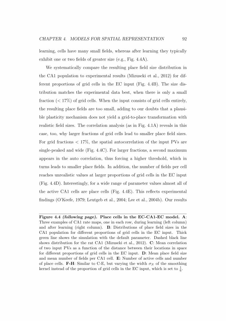
CHAPTER 4. MODELS FOR SPATIAL REPRESENTATION 92
learning, cells have many small fields, whereas after learning they typically
exhibit one or two fields of greater size (e.g., Fig. 4.4A).
We systematically compare the resulting place field size distribution in
the CA1 population to experimental results (Mizuseki et al., 2012) for dif-
ferent proportions of grid cells in the EC input (Fig. 4.4B). The size dis-
tribution matches the experimental data best, when there is only a small
fraction (< 17%) of grid cells. When the input consists of grid cells entirely,
the resulting place fields are too small, adding to our doubts that a plausi-
ble plasticity mechanism does not yield a grid-to-place transformation with
realistic field sizes. The correlation analysis (as in Fig. 4.1A) reveals in this
case, too, why larger fractions of grid cells lead to smaller place field sizes.
For grid fractions < 17%, the spatial autocorrelation of the input PVs are
single-peaked and wide (Fig. 4.4C). For larger fractions, a second maximum
appears in the auto correlation, thus forcing a higher threshold, which in
turns leads to smaller place fields. In addition, the number of fields per cell
reaches unrealistic values at larger proportions of grid cells in the EC input
(Fig. 4.4D). Interestingly, for a wide range of parameter values almost all of
the active CA1 cells are place cells (Fig. 4.4E). This reflects experimental
findings (O’Keefe, 1979; Leutgeb et al., 2004; Lee et al., 2004b). Our results
Figure 4.4 (following page). Place cells in the EC-CA1-EC model. A:Three examples of CA1 rate maps, one in each row, during learning (left column)and after learning (right column). B: Distributions of place field sizes in theCA1 population for different proportions of grid cells in the EC input. Thickgreen line shows the simulation with the default parameter. Dashed black lineshows distribution for the rat CA1 (Mizuseki et al., 2012). C: Mean correlationof two input PVs as a function of the distance between their locations in spacefor different proportions of grid cells in the EC input. D: Mean place field sizeand mean number of fields per CA1 cell. E: Number of active cells and numberof place cells. F-H: Similar to C-E, but varying the width σN of the smoothingkernel instead of the proportion of grid cells in the EC input, which is set to 1
6 .
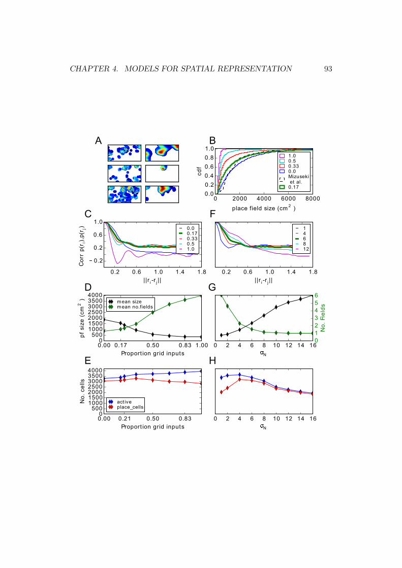
CHAPTER 4. MODELS FOR SPATIAL REPRESENTATION 93
A
0 2000 4000 6000 8000
place field size (cm2
)
0.0
0.2
0.4
0.6
0.8
1.0
cd
f
B
1.00.50.330.0Mizuseki et al.0.17
0.2 0.6 1.0 1.4 1.8
||r i -r j ||
0.2
0.2
0.6
1.0
Co
rrp(r
i),p
(rj)
C
0.00.170.330.51.0
0.2 0.6 1.0 1.4 1.8
||r i -r j ||
F
146812
0.00 0.17 0.50 0.83 1.00
Proport ion grid inputs
0500
1000150020002500300035004000
pf
siz
e (
cm
2)
D
m ean sizem ean no.fields
0 2 4 6 8 10 12 14 16
N
G
0
1
2
3
4
5
6
No
. Fie
lds
0.00 0.21 0.50 0.83
Proport ion grid inputs
0500
1000150020002500300035004000
No
. ce
lls
E
act iveplace_cells
0 2 4 6 8 10 12 14 16
N
H
CHAPTER 4. MODELS FOR SPATIAL REPRESENTATION 94
suggest that < 17% of EC inputs consists of grid cells, which is consistent
with data from the rat. Roughly half of the EC consists of MEC and about
one third of MEC cells projecting to the hippocampus are grid cells (Zhang
et al., 2013). Therefore, grid cells account for about 1/6 of EC cells in the
rat.
Given the relative importance of weakly spatially modulated cells in gen-
erating realistic place field sizes, we further investigate the dependence on
their properties, in particular the width of the smoothing kernel σN (see Sec-
tion 2.4.3 in Methods). For the following analysis, we fix the proportion of
grid cells at 1/6. If the kernel is narrow, the rate maps appear salt-and-
pepper-like (Fig. 2.6A) and the spatial autocorrelation is therefore rather
narrow and dominated by the grid inputs (Fig. 4.4F, blue and red lines). As
a result, the field sizes are small, the mean number of fields per cell is signif-
icantly larger than one (Fig. 4.4G) and very few of the active cells are place
cells (Fig. 4.4H). On the other hand, the autocorrelation of PVs is wide for
larger kernel width. Consequently, the mean size of hippocampal place fields
is larger in these simulations, there are fewer fields per cell (Fig. 4.4G) and
almost all active cells are place cells (Fig. 4.4H). We choose an intermediate
value of σN = 6 cm as a default, since it also roughly matches the spatial
information measured in LEC cells (Hargreaves et al., 2005), but note that
the exact procedure for generating the weakly modulated cells is not im-
portant for the model to replicate realistic place field sizes, only the spatial
autocorrelation of PVs matters.
4.2.2 Lesion studies
Since robustness is an important property of information processing in the
brain and since place cells are prominent for their robust firing in lesion

CHAPTER 4. MODELS FOR SPATIAL REPRESENTATION 95
0 400 800
no. lesioned cells
0.0
0.2
0.4
0.5
err
or
rate
A
LEC lesionsMEC lesionsG id l i
BNo LEC MEC Grid
No LEC MEC Grid0.0
0.5
1.0
1.5
2.0
no
. fi
eld
s
C
No LEC ME0.00
0.05
0.10
0.15
0.20
pf
siz
e (
m2
)
D
Figure 4.5. Effect of lesioning different EC inputs. A: Examples of ratemaps of three CA1 cells, one per row. Columns show rate maps when no lesion isapplied, the entire LEC is lesioned, the entire MEC is lesioned and when all gridcells are lesioned. B: Error rate as a function of the number of lesioned cells. C-E:Mean number of fields (C), place field size (D) and number of active cells whendifferent EC inputs are lesioned.
studies, we next examine the model’s sensitivity to lesioning different types
of EC inputs after the transformation has been learned. Place fields appear
largely preserved when all MEC, all grid cells or all LEC cells are lesioned
(Fig. 4.5A).
A systematic study, in which different fractions of input cells are le-
sioned selectively, reveals that place cells in our model are robust to le-
sions in the LEC and in the MEC, and is sensitive to specific lesions of grid

CHAPTER 4. MODELS FOR SPATIAL REPRESENTATION 96
cells (Fig. 4.5B). By adding grid cells, the model becomes more sensitive to
noise than a model that receives only weakly spatially modulated cells (green
dashed line in Fig. 4.5B), confirming the analysis in Figure 4.2.
Experimental studies indicate that, in MEC-lesioned rats, hippocampal
place cell responses continue to be spatially selective in familiar environments,
although their fields are broader and fewer cells are active (Brun et al., 2008;
Hales et al., 2014). We therefore study place field properties after EC lesions
in our model. If the entire MEC is lesioned it continues to generate rate maps
similar to those when the MEC input is present (Fig. 4.5A), but the number
of fields decreases slightly (Fig. 4.5C), field sizes are larger (Fig. 4.5D) and
the number of active cells is smaller (Fig. 4.5E). These modelling results
are in good qualitative agreement with the experimental observations. If
grid cells in MEC are selectively lesioned in our model, very similar effects
result, suggesting that the experimental effect might be due to the absence
of, specifically, grid cell firing. Complete lesions to the LEC lead to contrary
effects. Number of fields increase and sizes decrease, which can be explained
by the resulting higher grid cell proportion in the input. To conclude, the
EC-CA1-EC model creates place cells that have realistic place field sizes, are
robust and change their fields similarly as observed in lesion studies.
4.2.3 Stability
Next, we tested the stability of CA1 place fields. Hippocampal place cells
and cells in the MEC appear to have stable spatial firing maps during one
recording session and between session in the same environment (Thomp-
son and Best, 1990; Hargreaves et al., 2005; Yoganarasimha et al., 2011;
Mizuseki et al., 2012). By contrast, spatial firing is significant less stable
in LEC neurons especially in object-poor environments. Since LEC stabil-

CHAPTER 4. MODELS FOR SPATIAL REPRESENTATION 97
0.2 0.6 1.0
Stability LEC
0.2
0.6
1.0
Sta
bilit
y C
A1
A
No lesionLEC lesionMEC lesionGrid cell lesion
0.2 0.6 1.0
Stability LEC
1000
3000
5000
field
siz
e (
cm
2)
B
0.2 0.6 1.0
Stability LEC
0.5
1.5
No.
Fie
lds
C
0.2 0.6 1.0
Stability LEC
500
1500
2500
3500
cells
D
Figure 4.6. Stability of place cells. A: Stability of CA1 place cells betweentwo visits of the same environment as a function of stability in the LEC. Coloursindicate lesions of different entorhinal inputs before animal encounters the envi-ronment the second time. Error bars show standard errors of 5 simulations. B:Mean CA1 place field size, C:Mean number of place fields and D: Mean numberof active cells.

CHAPTER 4. MODELS FOR SPATIAL REPRESENTATION 98
ity seems to depend on the properties of the environment, we parametrized
the level of LEC stability (see Section 2.5.6 in Methods). We find that the
model produces stable place fields with a constant field size for all stability
levels (Fig. 4.6A,B, black lines). Also the number of active cells were con-
stant. Furthermore, lesioning the MEC leads to lower hippocampal stability,
larger place fields, and lower number of active cells. These effects are more
pronounced when LEC stability is low. Lesioning the LEC had only minor
effects. Thus, the pattern of stability in the model is in good qualitative
agreement with experimental findings obtained in object poor environments
(Lu et al., 2013; Hales et al., 2014). Moreover, our model predicts that the
effects of MEC lesions on hippocampal place field size, stability, and number
of active cells are reduced in object rich environments, when LEC activity is
more stable.

Chapter 5
Discussion
5.1 Summary
5.1.1 Memory formation in the hippocampus
The thesis started by reviewing the standard model of memory formation.
We compared three different models: the standard model itself, the standard
model without recurrent connections and the minimal EC-CA1-EC model.
In doing so we investigated the models’ ability to store input patterns of three
different kinds: random patterns, grid cell patterns and patterns of grid cells
and weakly spatially modulated cells.
Surprisingly, we find that when random inputs are stored an auto-
associative CA3 network is redundant for pattern completion of recall cues
with strong and moderate cue strength. It is only helpful for highly distorted
cues, but this advantage comes with the prize of a higher confusion rate of
cues with wrong patterns. Moreover, the network is even harmful for all cue
strengths when inputs of grid cells or inputs of grid cells and weakly spatially
modulated cells are stored, which we regard as biologically more plausible
99

CHAPTER 5. DISCUSSION 100
inputs. In these cases, the minimal EC-CA1-EC model is most efficient in
pattern completion and confuses cues less often despite its simplicity. We
further provide an intuition why this simpler network performs best.
Moreover, we find that Hebbian plasticity in the synapses from EC to DG
does not support pattern separation in the DG as suggested by the standard
model. With the biologically more plausible inputs Hebbian plasticity has
even the opposite effect.
These results challenge the standard model. In particular, they question
its crucial idea that an auto-associative CA3 network performs pattern com-
pletion. Instead, they suggest that pattern completion is rather performed
in a feedforward way by the simpler EC-CA1-EC model.
5.1.2 Hippocampal place cell formation out of grid
cells
Next we investigated place cell formation out of grid cell input in the dorsal
hippocampus. We pointed out that all feedforward grid-to-place models gen-
erate either highly non robust place cells or place cells that have only small
place fields. We studied this issue in a generic feedforward model, which is a
general version of the feedforward networks discussed in the literature. We
find that the creation of realistically sized fields is implausible due to the
structured spatial autocorrelation of the grid input and hence not due to an
improper parameter tuning in the individual models.
We then asked whether the feedforward transformation from grid input
to place cells with realistic field sizes is possible at all by applying different
machine learning algorithms to the generic model. We find that there are
transformations, but these transformation are biologically not plausible for
to two reasons. Firstly, large place cells are highly sensitive to noise in these

CHAPTER 5. DISCUSSION 101
transformations contradicting their robustness. Secondly, these transforma-
tions rely mainly on grid cells with large spacings. However, these cells are
by far outnumbered by grid cells with small spacings in the dorsal MEC.
Moreover, it is highly speculative whether these transformations found by a
computer algorithm can be learned in a biologically plausible self-organized
way. Thus, our results suggest that place cells are not solely driven by grid
cells in a feedforward network and that further mechanisms have to be added
to account for experimentally observed place fields.
5.1.3 Place cell formation in the EC-CA1-EC model
We propose that place cells are generated by a mixture of grid cells and other
cells that are present in the EC and tested this hypothesis in the EC-CA1-
EC model. Entorhinal cells that are not grid cells are modelled abstractly as
weakly spatially modulated cells carrying only little spatial information. We
investigated place cell formation by Hebbian learning given different inputs.
We find that given only grid cell input, place cells have unrealistically
many and small place fields confirming our analysis above. More interest-
ingly, when the input consists of a mixture of grid cells and weakly spatially
modulated cells, the model produces place cells with realistic characteristics
such as place field size, average number of fields per cell and robustness to
input perturbations for a wide parameter range. In particular, this is true
for a mixture that consist of a grid cell proportion of 1/6, which reflects
experimental estimates of the amount of hippocampal grid cell input. This
supports our suggestion that place cells are triggered by a mixture of grid
cells and non-grid cells.
We further studied place field properties in the model after lesioning sev-
eral entorhinal regions. We find that after MEC lesions fewer place cells
CHAPTER 5. DISCUSSION 102
are active and place fields become broader, which is in good agreement with
the puzzling findings in experimental lesion studies performed in rats (Brun
et al., 2008; Hales et al., 2014; Ormond and McNaughton, 2015). Further-
more, the model makes some strong predictions regarding LEC and grid cell
lesions in novel and familiar environments.
Since LEC cells are relatively temporally unstable, we studied whether
this instability affects the stability of place cells. Due to the stability provided
by MEC cells and the robustness of the model we find stable place cell firing
in CA1 even for highly unstable LEC cells. Moreover, lesioning different
parts of the EC in the model lead to similar behaviour of place cell stability as
observed in experiments obtained in object poor environments. Furthermore,
the model makes predictions regarding place field sizes, place field stability
and number of active cells in object rich environments, where LEC cells are
more stable.
These results support the idea that place cells are mainly triggered by
non-grid cells including cells from the LEC despite their lack of stability and
spatial information.
5.2 Detailed discussion
5.2.1 Issues with the standard model
In the last decades, a view has evolved about how the peculiar anatomic
structure of the hippocampus serves memory formation. It has been postu-
lated that the CA3 region with its many recurrent connections functions as
an attractor network performing pattern completion when degraded input
is given (McNaughton and Morris, 1987; Rolls, 2007). Thus, it is believed
that CA3 is the actual storing place. Complex mathematical analysis show

CHAPTER 5. DISCUSSION 103
that the memory capacity of such a network is sufficient, when the activ-
ity in the region is sparse enough (Hopfield, 1982; Amit, 1989; Treves and
Rolls, 1991). However, a decorrelation among the stored patterns is crucial
and all the analysis supposes that. It is believed that the DG removes all
correlations from the input patterns of the EC and performs the so called pat-
tern separation. This is supported by a sparse coding, by strong and sparse
synapses from DG to CA3 (O’Reilly and McClelland, 1994; Rolls, 2007), and
by Hebbian plasticity from EC to DG during storage (Rolls, 1995).
In Chapter 3 we challenge this view and show several weaknesses of it.
Firstly, in the mathematical analysis of the standard framework only an iso-
lated CA3 network has been considered and the inevitable decoding pathway
via CA1 has been neglected. We show that this pathway is capable of re-
constructing the memory even when the recurrent connections in CA3 are
removed. This makes the assigned auto-associative function of CA3 redun-
dant for low to moderate noise levels. Interestingly, by arguing for CA3 being
an attractor network, Treves and Rolls (1991) compared the ability of pattern
completion of an auto-associative network with that of subsequent hetero-
associative networks (Treves and Rolls, 1991). They conclude that when the
sparsity of the activity approaches zero, the performance of a single auto-
associative memory reaches nearly that of several hetero-associations, while
at the same time fewer neuronal components are needed. However, in the
standard model these components have to be present to perform encoding
and decoding, turning this argument against the proposed function of CA3.
Thus, our work illustrates how essential it is to consider the whole hippocam-
pal loop while investigating individual functional roles of the subregions.
Secondly, simple Hebbian plasticity in the DG as proposed by Rolls (1995)
does not support pattern separation. To the contrary. We have shown that
CHAPTER 5. DISCUSSION 104
due to this plasticity the grid cell code in the EC is mapped onto a place
field like code in CA3. This is in line with other work, that investigate
the transformation from grid cells to place cells (Rolls et al., 2006; Franzius
et al., 2007; Si and Treves, 2009; Savelli and Knierim, 2010; Cheng and Frank,
2011) by Hebbian learning. In this code, patterns from nearby locations
happen to be highly correlated, which is the opposite of what a pattern
separator should do. Thus, a competitive net is not a good candidate to
orthogonalize patterns for grid cell input. What is not modelled here, is
adult neurogenesis in the DG (Gross, 2000). This additional plasticity might
support pattern separation in contrast to Hebbian learning alone. Weisz and
Argibay (2009) studied the effects of neurogenesis in the standard model
and they find advantages in memory performance, but they only considered
the case of random inputs (Weisz and Argibay, 2009). However, alternative
hypotheses for adult neurogenesis exist (e.g (Appleby et al., 2011)). We show
that by having random and fixed connections the DG performs quite well as
a pattern separator. Only for very highly correlated patterns in the input,
there remains some amount of correlation in these patterns after applying the
separator. Despite the significant reduction, this amount is still enough to
degrade the auto-associative CA3. Thus, to make the standard model work,
a separator is needed that functions perfectly. However, assuming it exists,
the benefit of a recurrent CA3 net would still be small compared to the EC-
CA1-EC model if applied to grid cell input (compare red line in Fig. 3.3E
with magenta line in Fig. 3.8F).
Thirdly, a further challenging argument against an auto-associative func-
tion of CA3 is the fact that the actual representations in the mammalian
CA3 are far from uncorrelated. The vast majority of active pyramidal cells
are place cells (O’Keefe, 1976), thus activity patterns are correlated by na-

CHAPTER 5. DISCUSSION 105
ture. Storing such patterns of continuous place cell activity that occur in one
environment in an auto-associative network leads to a continuous attractor
or so called chart (Samsonovich and McNaughton, 1997; Cerasti and Treves,
2013). Every point in this chart refers to the neural representation of one
location in the environment. A degraded input is then attracted towards
a point on the chart and the network is indeed able to diminish the noise
orthogonal to the attractor. However, it has been observed that many points
are not stable (Tsodyks and Sejnowski, 1995) and drift along the attractor
until they reach a fixed point (Cerasti and Treves, 2013). This means that
many patterns finally retrieved are representations of the wrong location.
The issue of drifting is even more pronounced when discrete memories are
stored on top of the continuous chart. In this case only a fraction of lo-
cations are stable (Roudi and Treves, 2008; Solstad et al., 2014). Since we
store correlated patterns in the auto-associative CA3 net, a continuous at-
tractor is also formed in the present model. It can store a large number of
patterns drawn from the grid map moderately well, however, drifting occurs
in the recall. This drifting is already reduced, since the CA3 representations
are binary rather than continuous (Papp et al., 2007), but still apparent as
reflected by the high confusion rate of patterns when using the recurrent con-
nections in CA3 (see Fig 3.7C). Papp et al.(2007) state that the drift may be
much slower than pattern completion and hence storage of locations is still
possible (Papp et al., 2007). In other words, pattern completion is already
done in the first update cycles in the attractor network. This is in agreement
with our results. By viewing each hetero-associative step as one update cy-
cle, pattern completion is performed by the two hetero-associative networks
EC-CA1 and CA1-EC without loosing accuracy caused by the drift and the
auto-associative function in CA3 becomes redundant. Consequently, given

CHAPTER 5. DISCUSSION 106
the structured grid cell input in the EC, the simpler network EC-CA1-EC is
already sufficient for pattern completion and it confuses memories less often
than the more complex standard model does.
5.2.2 Alternative functions for CA3
We established that a recurrent CA3 is not necessary for pattern completion.
This frees the recurrent CA3 connections to perform other functions. For in-
stance, Levy (1996) suggested that CA3 associates its present activity with
activity occurring in the past . In this way, sequences of activities are stored,
which can explain the hippocampal involvement in tasks like trace condition-
ing or configural learning problems. A further alternative to an attractor net
in CA3 has been suggested by Cheng (2013). He assumes that the recurrent
CA3 network is not plastic, but rather creates intrinsic sequences which are
then associated with temporal sequences of patterns in the EC .
We do not model temporal aspects here, but our study shows that because
of the redundancy of CA3 as an auto-associative net, it very likely fulfils
some other function. Similarly, the EC-CA1-EC model does not require
plasticity in the synapses projecting from EC to CA3 nor in the Schaffer
Collaterals, where plasticity has been found (Buchanan and Mellor, 2010,
for a review). Hence, the plasticity could serve another function leaving the
pattern completion function in the EC-CA1-EC model unaffected.
5.2.3 Evidence for pattern completion in CA3?
Experimental studies reported putative evidence for CA3 being an auto-
association memory. For example, Gold and Kesner (2005) show that rats
with lesioned CA3 are impaired in remembering a location when parts of the
spatial cues are removed (Gold and Kesner, 2005). Another study obtains

CHAPTER 5. DISCUSSION 107
similar results when plasticity in CA3 synapses is corrupted in knock-out
mice (Nakazawa et al., 2002). The authors conclude that CA3 is crucial for
spatial pattern completion. In our opinion this is not convincing. If the ac-
tual location of the memory is CA3 then lesioning it or removing plasticity
should give equivalent results as lesioning the entire hippocampus (Cheng,
2013). This is not the case, since in both studies animals behave normally in
full cue conditions, but animals with hippocampal lesions are clearly impaired
(Morris et al., 1982; Gilbert et al., 1998). An alternative interpretation for
the experimental observations could be that the animals rely more on the
integration of self motion cues in conditions when external cues are poor.
This is in line with others who assign a path integration function to CA3
(Samsonovich and McNaughton, 1997; Colgin et al., 2010). If spatial infor-
mation provided by the external cues is sufficient, spatial recognition can be
performed by CA1 alone (Brun et al., 2002; Steffenach et al., 2002).
In another experimental paradigm CA3 and CA1 population activities are
compared in a familiar radial maze with the activities in an altered version of
the maze when local and distal cues have been rotated in opposite directions
(Lee et al., 2004a). It has been shown that CA3 cells follow the local cue
rotation coherently, where this is not seen in CA1. Thus, CA3 is capable
to restore the original representations (rotated by the local cues) despite the
noisy sensory inputs caused by the conflicting rotation of the global cues.
The authors interpret this is as strong evidence for pattern completion in
CA3.
In our opinion this interpretation is imprecise. The study does not show
that CA3 receives noisy representations as direct input and it is possible that
the observed pattern completion is already performed in one of its upstream
regions. Although CA1 representations do not show high correlation between
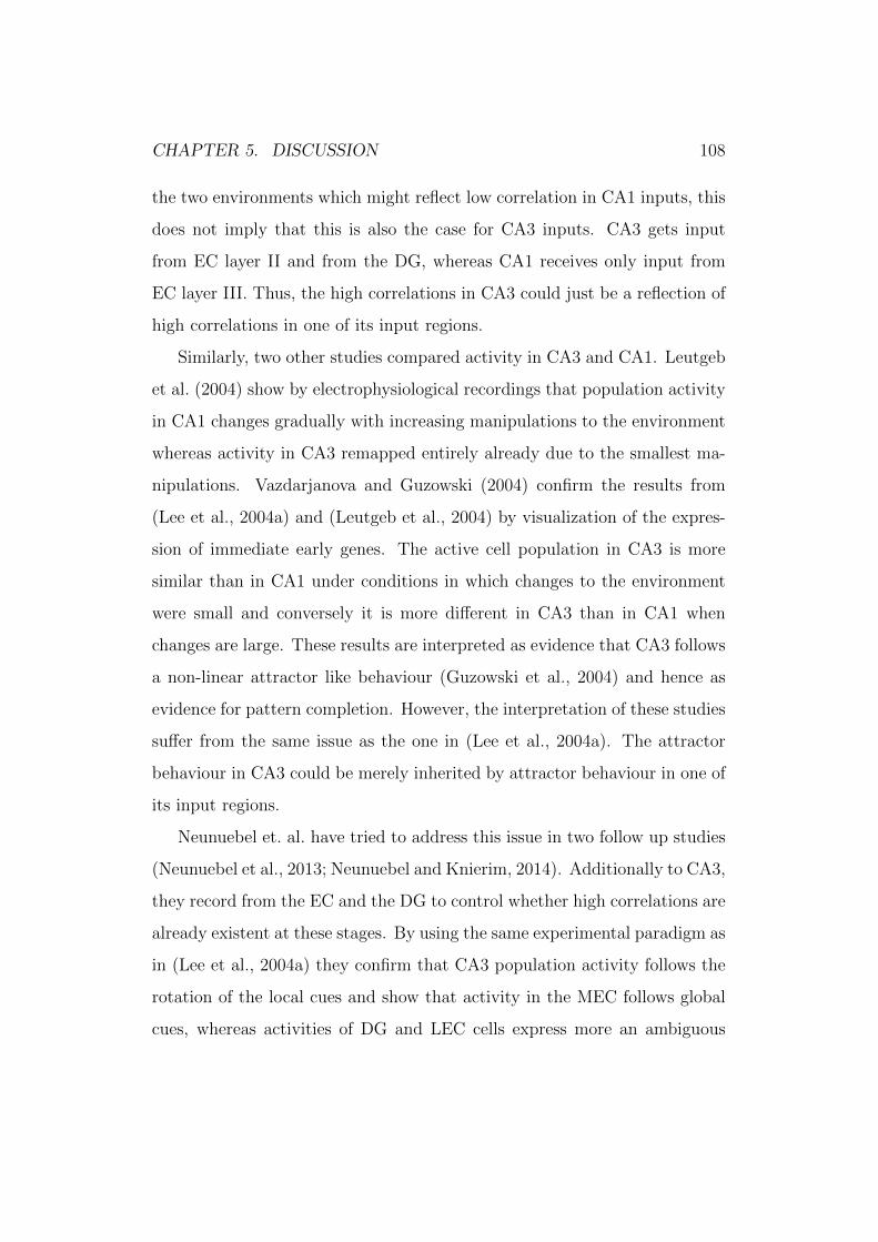
CHAPTER 5. DISCUSSION 108
the two environments which might reflect low correlation in CA1 inputs, this
does not imply that this is also the case for CA3 inputs. CA3 gets input
from EC layer II and from the DG, whereas CA1 receives only input from
EC layer III. Thus, the high correlations in CA3 could just be a reflection of
high correlations in one of its input regions.
Similarly, two other studies compared activity in CA3 and CA1. Leutgeb
et al. (2004) show by electrophysiological recordings that population activity
in CA1 changes gradually with increasing manipulations to the environment
whereas activity in CA3 remapped entirely already due to the smallest ma-
nipulations. Vazdarjanova and Guzowski (2004) confirm the results from
(Lee et al., 2004a) and (Leutgeb et al., 2004) by visualization of the expres-
sion of immediate early genes. The active cell population in CA3 is more
similar than in CA1 under conditions in which changes to the environment
were small and conversely it is more different in CA3 than in CA1 when
changes are large. These results are interpreted as evidence that CA3 follows
a non-linear attractor like behaviour (Guzowski et al., 2004) and hence as
evidence for pattern completion. However, the interpretation of these studies
suffer from the same issue as the one in (Lee et al., 2004a). The attractor
behaviour in CA3 could be merely inherited by attractor behaviour in one of
its input regions.
Neunuebel et. al. have tried to address this issue in two follow up studies
(Neunuebel et al., 2013; Neunuebel and Knierim, 2014). Additionally to CA3,
they record from the EC and the DG to control whether high correlations are
already existent at these stages. By using the same experimental paradigm as
in (Lee et al., 2004a) they confirm that CA3 population activity follows the
rotation of the local cues and show that activity in the MEC follows global
cues, whereas activities of DG and LEC cells express more an ambiguous
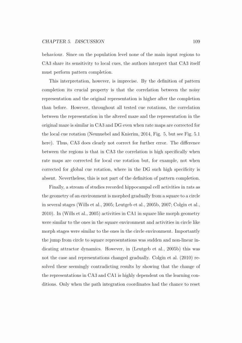
CHAPTER 5. DISCUSSION 109
behaviour. Since on the population level none of the main input regions to
CA3 share its sensitivity to local cues, the authors interpret that CA3 itself
must perform pattern completion.
This interpretation, however, is imprecise. By the definition of pattern
completion its crucial property is that the correlation between the noisy
representation and the original representation is higher after the completion
than before. However, throughout all tested cue rotations, the correlation
between the representation in the altered maze and the representation in the
original maze is similar in CA3 and DG even when rate maps are corrected for
the local cue rotation (Neunuebel and Knierim, 2014, Fig. 5, but see Fig. 5.1
here). Thus, CA3 does clearly not correct for further error. The difference
between the regions is that in CA3 the correlation is high specifically when
rate maps are corrected for local cue rotation but, for example, not when
corrected for global cue rotation, where in the DG such high specificity is
absent. Nevertheless, this is not part of the definition of pattern completion.
Finally, a stream of studies recorded hippocampal cell activities in rats as
the geometry of an environment is morphed gradually from a square to a circle
in several stages (Wills et al., 2005; Leutgeb et al., 2005b, 2007; Colgin et al.,
2010). In (Wills et al., 2005) activities in CA1 in square like morph geometry
were similar to the ones in the square environment and activities in circle like
morph stages were similar to the ones in the circle environment. Importantly
the jump from circle to square representations was sudden and non-linear in-
dicating attractor dynamics. However, in (Leutgeb et al., 2005b) this was
not the case and representations changed gradually. Colgin et al. (2010) re-
solved these seemingly contradicting results by showing that the change of
the representations in CA3 and CA1 is highly dependent on the learning con-
ditions. Only when the path integration coordinates had the chance to reset

CHAPTER 5. DISCUSSION 110
Figure 5.1. No pattern completion in CA3 in the double cue rotationtask. Each red (blue) polar plot in the left (right) column shows the mean spatialcorrelation between CA3 (DG) PVs in the unaltered environment and PVs in thealtered environment as a function of spatial rotation of the cells’ rate maps inthe altered environment. Each row shows an experiment where the degree of cuerotations of the altered environment were different. L indicates the degree of localcue rotation and G the degree of global cue rotation. Numbers on the left showthe degree of total cue rotation, i.e. in the experiment of the first row, local cueswere rotated 22.5 degrees counter clockwise and global cues 22.5 degrees clockwise.Black dots indicate angles of rate map rotations at which mean correlations wheremaximal. Note that the correlations in CA3 were specifically high when rate mapsare rotated to the same degree as the local cues. In the DG, this high specificityis not seen. However, the amount of correlation is not higher in CA3 than DGeven when rate maps are rotated according to local cue rotation. Grey polar plotsshow control experiment when the rat enters the same environment twice. Figureis taken with permission from (Neunuebel and Knierim, 2014, Fig.5)
.

CHAPTER 5. DISCUSSION 111
during learning the representations of the circle and square environment, the
jump in representations will be sudden during testing. Thus, attractor like
behaviour in CA3 is very likely due to the path integration system, which
is believed to originate in the MEC (McNaughton et al., 2006). Hence, it
seems that the MEC is the source for the sudden change in hippocampal cell
activity and not the putative auto-associative CA3 network. Indeed, (Fyhn
et al., 2007) show that global remapping (a sudden change of hippocam-
pal representations) is accompanied by remapping of grid cells in the MEC.
Moreover, Leutgeb et al. (2007) show that when there is a gradual shift in
CA3 activity in the morphing paradigm, grid cell activity is stable. Thus,
the MEC is likely to be the source of the observed attractor dynamics in
the hippocampus and not CA3, although there are models that explain rate
remapping in the morphing experiment through feedback connections in CA3
(Renno-Costa et al., 2014; Solstad et al., 2014).
To conclude, although otherwise claimed, up to date there is no clear
evidence of pattern completion in CA3. Carefully examination of work that
postulates such evidence reveals imprecise interpretations or opens up alter-
native explanations of the observed data.
5.2.4 Grid cells as the only source for place cells is
implausible
The firing behaviour of grid cells and place cells is correlated in many ways.
First, both cell types are similarly dependent on landmarks and boundaries of
the environment. Both exhibit stable firing patterns during repeated visits
of the same environment (Thompson and Best, 1990), are robust to the
removal of some environmental cues (O’Keefe and Conway, 1978; Hafting
et al., 2005) and mainly preserve their firing maps during darkness (Quirk

CHAPTER 5. DISCUSSION 112
et al., 1990; Zhang et al., 2014). Moreover, when prominent landmarks are
moved, both types rotate their firing patterns in concert with the displaced
landmark (Muller and Kubie, 1987; Hafting et al., 2005), however, grid cells
follow global cues and place cells mainly local cues in conflicting rotations
(Neunuebel et al., 2013; Neunuebel and Knierim, 2014). Finally, when the
boundaries of a familiar environment are expanded, the size of the place
fields in both cell types rescale, too (O’Keefe and Burgess, 1996; Barry et al.,
2007).
Second, the field sizes in both types increase along the dorsal to ventral
axis (Fyhn et al., 2007; Kjelstrup et al., 2008) and the connection from EC
to hippocampus is topographic along this axis (Dolorfo and Amaral, 1998;
Honda et al., 2012), i.e dorsal EC cells project mostly to the dorsal hip-
pocampus and ventral cells mostly to the ventral hippocampus.
Third, when the animal encounters a novel environment for the first time,
place fields in both types tend to be larger during the first minutes of exposure
(Mehta et al., 1997; Lee et al., 2004a; Barry et al., 2012). However, the time
scale until stable size is reached might differ.
Finally, global remapping in the hippocampus appears to happen exactly
when grid cells remap (Fyhn et al., 2007; Barry et al., 2012).
Consequently, it is suggested that both cell types are not just correlated,
but that this relationship is causal. In more detail, it is proposed that grid
cells are driving place cell activity (Fuhs and Touretzky, 2006; McNaughton
et al., 2006; Rolls et al., 2006; Solstad et al., 2006; Blair et al., 2007; Franzius
et al., 2007). A few experimental findings support this causality. CA1 place
cells are unstable in rats with a lesioned EC (Van Cauter et al., 2008), but are
stable when only LEC is lesioned (Lu et al., 2013) or when the input from
CA3 is blocked (Brun et al., 2002; Nakashiba et al., 2008). Furthermore,

CHAPTER 5. DISCUSSION 113
place fields at distal parts in CA1 are less spatial than the ones in proximal
parts (Nakamura et al., 2013). At the same time, distal parts receive less
input from the MEC (Honda et al., 2012) and hence probably receive less
input from grid cells.
However, other experimental work questions the plausibility of such
causality (Bush et al., 2014). Lesions to the MEC of rats did not abolish
place cell firing (Brun et al., 2008; Hales et al., 2014). Second, two develop-
mental studies have shown that in young rat pups place and head-direction
cells developed adult like firing patterns earlier than grid cells do (Wills
et al., 2010; Langston et al., 2010). Third, in other studies, theta oscilla-
tion in the hippocampus was disrupted by reversibly inactivating the medial
septum (Koenig et al., 2011; Brandon et al., 2011, 2014). This resulted in a
high degradation of the periodicity in grid cell firing, but at the same time
CA1 place cells continued to have normal fields. However, in large and novel
environments place cell firing was disrupted under these conditions (Wang
et al., 2015). Forth, it has been shown that in conflicting cue rotations cells
in the MEC mainly follow global cues and CA3 place cells mainly local cues
(Neunuebel et al., 2013; Neunuebel and Knierim, 2014). Fifth, place fields
in grid and place cells are larger in first entries to novel environments, but
this expansion last for hours in grid cells (Barry et al., 2012), whereas place
cells become stable much more rapidly (Mehta et al., 1997; Lee et al., 2004a).
Finally, it has been shown that cells in the MEC fire shortly after pyramidal
cells in the hippocampus, making a casual relationship unlikely (Mizuseki
et al., 2009).
Although some of these issues could be accounted for by robustness of the
grids-to-places transformation (Azizi et al., 2014), the experimental evidence
whether grid cells trigger place cells remains unclear. In this thesis we have

CHAPTER 5. DISCUSSION 114
pointed out that a linear grid-to-place transformation suffers from another
issue that has received little attention so far: unrealistically small place field
sizes.
Theoretical work that models this transformation produces place fields
that have either small sizes reflecting those fields found in the granule cells
in the DG (Rolls et al., 2006; Solstad et al., 2006; Si and Treves, 2009;
de Almeida et al., 2009; Savelli and Knierim, 2010; Azizi et al., 2014) or fields
that are highly sensitive to tiny perturbations in the input (Blair et al., 2007).
One study explicitly models the formation of place fields in CA3 by mixing
grid cell input with input from the DG and by mimicking realistic distribution
of synapses (de Almeida et al., 2012). They are able to generate place cells
with single fields by using a competitive activation function, however, for all
investigated model parameters the fields were too small compared to CA3
fields found experimentally (de Almeida et al., 2012, see Fig. 4b).
Another modelling study suggested that a place cell is the result of a
Fourier transform where grid cells with a common spatial phase are the basis
functions (Solstad et al., 2006). To produce large place fields, the model
relies on grid cells with a grid spacing larger than any observed so far. One
prediction of the model is that lesioning grid cells with large spacings leads to
contraction of place fields, whereas lesions of cells with small spacings lead to
an expansion of fields. A recent study tested this prediction experimentally
by inactivating grid cells at three different locations along the dorsoventral
axis of MEC, along which grid spacings increase systematically (Ormond
and McNaughton, 2015). In contrast to the model predictions, inactivation
at all MEC locations result in an expansion of place fields. Moreover, the
number of place fields decreases. Interestingly, both experimental findings
are predicted by our EC-CA1-EC model that includes input from weakly

CHAPTER 5. DISCUSSION 115
spatially-modulated cells
In Section 4.1.1 we have provided a computational reason why feedfor-
ward models cannot produce realistically sized fields. The structured spatial
autocorrelation of the grid cell PVs prevents the formation of single large
fields. This spatial structure is enhanced when grid cells express a common
orientation (Solstad et al., 2006) and experiments indeed show that grid cell
orientations are clustered in rats (Barry et al., 2007; Stensola et al., 2012).
On the other hand, the grid symmetry reduces with increasing variety be-
tween the peak firing rates of the receptive fields of individual grid cells (Rolls
et al., 2006; Bush et al., 2014) and this variety has been found in rats (Hafting
et al., 2005). In our models we are rather conservative and grid cell orien-
tations are only clustered module wise and different modules have different
mean orientations distributed along the entire 0 to 60 degrees (Fig. 2.5C).
Moreover, we introduce some variety between peak firing rates of receptive
fields, too (see Section 1.4.1 in Methods). However, despite these symmetry
breaking aspects, our general feedforward model shows that the formation of
realistic place cells by grid cells is questionable.
To conclude, experimental studies tell us that place cells are present in
the absence of medial entorhinal input and in particular of grid cell input.
Moreover, we have provided theoretical evidence that a grid-to-place trans-
formation simply by a feedforward network is implausible. This strengthen
alternatives models for place cell formation that do not rely solely on grid
cells or models that are not purely feedforward.
5.2.5 Alternative models for place cell formation
The boundary vector cell (BVC) model suggests that place cell firing arise
through the input from border cells in the MEC (Hartley et al., 2000; Burgess
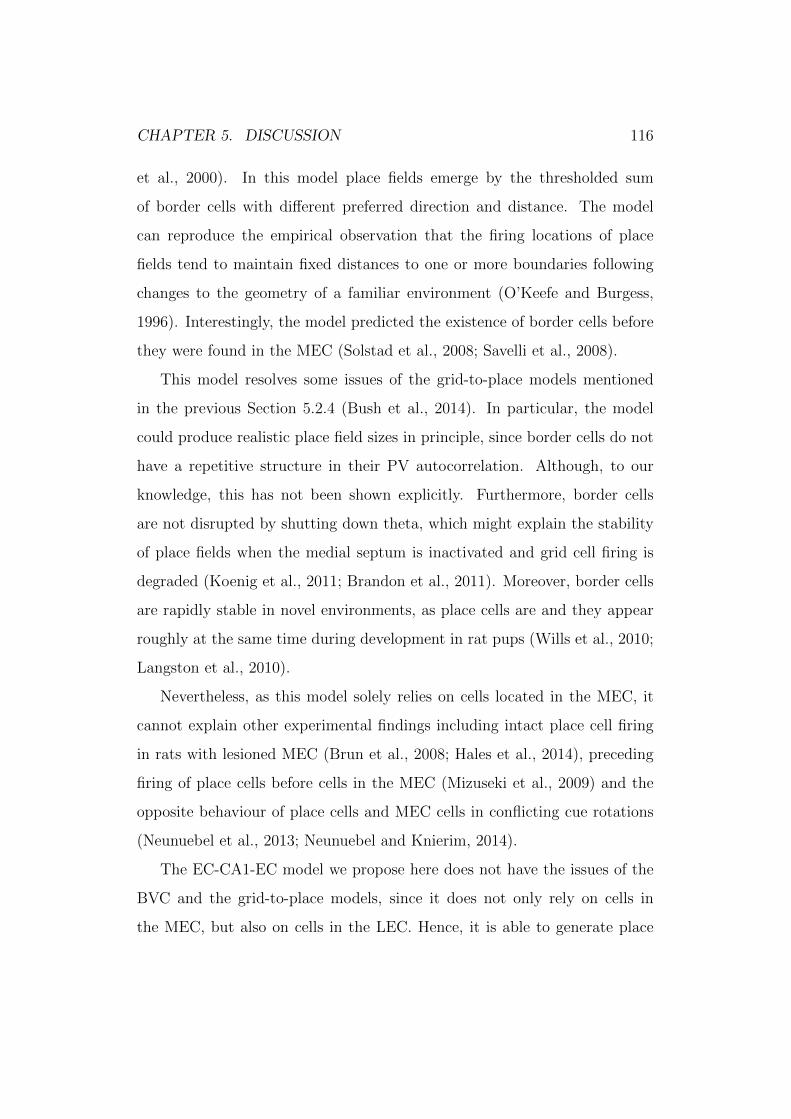
CHAPTER 5. DISCUSSION 116
et al., 2000). In this model place fields emerge by the thresholded sum
of border cells with different preferred direction and distance. The model
can reproduce the empirical observation that the firing locations of place
fields tend to maintain fixed distances to one or more boundaries following
changes to the geometry of a familiar environment (O’Keefe and Burgess,
1996). Interestingly, the model predicted the existence of border cells before
they were found in the MEC (Solstad et al., 2008; Savelli et al., 2008).
This model resolves some issues of the grid-to-place models mentioned
in the previous Section 5.2.4 (Bush et al., 2014). In particular, the model
could produce realistic place field sizes in principle, since border cells do not
have a repetitive structure in their PV autocorrelation. Although, to our
knowledge, this has not been shown explicitly. Furthermore, border cells
are not disrupted by shutting down theta, which might explain the stability
of place fields when the medial septum is inactivated and grid cell firing is
degraded (Koenig et al., 2011; Brandon et al., 2011). Moreover, border cells
are rapidly stable in novel environments, as place cells are and they appear
roughly at the same time during development in rat pups (Wills et al., 2010;
Langston et al., 2010).
Nevertheless, as this model solely relies on cells located in the MEC, it
cannot explain other experimental findings including intact place cell firing
in rats with lesioned MEC (Brun et al., 2008; Hales et al., 2014), preceding
firing of place cells before cells in the MEC (Mizuseki et al., 2009) and the
opposite behaviour of place cells and MEC cells in conflicting cue rotations
(Neunuebel et al., 2013; Neunuebel and Knierim, 2014).
The EC-CA1-EC model we propose here does not have the issues of the
BVC and the grid-to-place models, since it does not only rely on cells in
the MEC, but also on cells in the LEC. Hence, it is able to generate place

CHAPTER 5. DISCUSSION 117
cells even when the MEC is lesioned. We use a more abstract cell class, the
weakly spatially modulated cells, which do not systematically express firing
fields at borders. Their crucial property is that their population activity
does not have a repetitive structure. Border cells do not have such structure
either. Thus, when part of the weakly spatially modulated cells are modelled
more concretely, i.e. when a subset of these abstract cells is substituted by
border cells, the model should produce qualitatively similar place cells as
those observed in Section 4.2.1. However, by implementing border cells into
the model it could, as the BVC model, reproduce the experimental finding
that place field locations tend to appear at fixed distances to boundaries
(O’Keefe and Burgess, 1996).
Another possibility is that place cells are driven solely by grid cells but
in a more complex network. For example a model of CA3 with recurrently
connected neurons could generate realistically sized fields, even when CA3
cells receive only narrowly tuned spatial drive from grid cells (Neher et al.,
2015a). Due to the recurrence and the excitation by other neurons that
receive spatial inputs at a more distant location, the place field of a CA3
cell will appear larger than the extent of its external spatial input. However,
since this model does only rely on grid cells, it has all other issues of the
grid-to-place models described earlier.
In some previous feedforward models, non-spatial input was present in
addition to the grid cell input (Si and Treves, 2009). However, this had only
a small effect on the place field sizes and could not generate realistic field
sizes. Lyttle et al. (2013) modelled the increase of hippocampal place field
sizes along the dorsal to ventral axis by increasing the spacings of grid inputs
along this axis and also by increasing the amount of non-spatial inputs at
ventral locations. In this way, realistic place fields sizes could be generated

CHAPTER 5. DISCUSSION 118
Figure 5.2. Adding non-spatial inputs to grid cells might not be suffi-cient to generate realistic place cells. Plots show cumulative density functionsof place field sizes measured in the model of Lyttle et al. (2013) using differentparameters (green, red and blue lines) and field sizes measured in rats (black lines)(Royer et al., 2010). Left plot shows distributions in the dorsal hippocampus andright plot in the ventral hippocampus. Although the model could reproduce thesizes measured in the ventral hippocampus, the model generated for all parame-ters dorsal place field sizes that were too small indicating that grid cell input tothe dorsal hippocampus along with non-spatial input is not sufficient to generatedorsal place fields of realistic size. Figure is taken with permission from (Lyttleet al., 2013, Fig.5)
in the ventral hippocampus but not in the dorsal hippocampus (Lyttle et al.,
2013, Fig. 5A, but see Fig. 5.2 here). Hence, the results of these studies
suggest that non-spatial inputs along with grid inputs are not sufficient to
produce realistic place fields in a feedforward network.
We suggest instead that place cells are generated by a mixture of grid
cells and cells that are somewhat spatial and carry at least some spatial
information. These cells are abundant in the MEC (Zhang et al., 2013)
and in particular in the LEC (Hargreaves et al., 2005; Yoganarasimha et al.,
2011). We have shown that this mixture is sufficient to generate realistically
sized place fields in a feedforward network. Interestingly, in the conflicting

CHAPTER 5. DISCUSSION 119
cue rotation task LEC cells tend to follow local cues (Neunuebel et al., 2013)
similar to place cells in CA3 (Neunuebel and Knierim, 2014), which indicate
their influence on hippocampal place cell formation.
To conclude, to our knowledge the EC-CA1-EC model is the first model
that produces robust place cells with realistic field sizes and that is in good
agreement with puzzling results from a large body of experimental studies
(Brun et al., 2008; Wills et al., 2010; Langston et al., 2010; Koenig et al.,
2011; Brandon et al., 2011; Mizuseki et al., 2012; Zhang et al., 2013; Brandon
et al., 2014; Hales et al., 2014; Ormond and McNaughton, 2015, for example).
Thus, the model presented supports the view that grid cells and cells in the
MEC are not the only source for place cell formation and that rather cells
across the entire EC are involved, despite their lack of spatial information
and stability.
5.2.6 Role of grid cells
If, as our results suggest, grid cells are not sufficient for the creation of place
fields of realistic size in the hippocampus, are they necessary for place cell
firing at all? In the absence of external visual inputs, place cells can maintain
their firing location (Quirk et al., 1990; Gothard et al., 1996; Zhang et al.,
2014). Thus, in addition to external cues, place cells also receive positional
information from self-motion cues and likely grid cells are the source of this
information. It is has been suggested that grid cells are part of a path
integration system in the MEC that updates positional information based on
self-motion cues (McNaughton et al., 2006). Their regular hexagonal pattern
of firing fields might provide the distance metric, medial entorhinal head
direction cells the directional information and the recently founded speed
cells in the MEC (Kropff et al., 2015) might provide the information about

CHAPTER 5. DISCUSSION 120
the animals velocity. Thus, the MEC has all the neural components necessary
for performing path integration. Indeed, all three cell types maintain their
firing behaviour during darkness (Taube et al., 1990a; Hafting et al., 2005;
Kropff et al., 2015).
On the other hand, cells in the LEC are receptive to individual sensory
cues such as objects or odours (Zhu et al., 1995b,a; Young et al., 1997; Desh-
mukh and Knierim, 2011) and in object-poor environments their rate maps
are less stable over time as compared to cells in the MEC (Hargreaves et al.,
2005; Yoganarasimha et al., 2011). Thus, when external cues are weak, tem-
poral stability of place cells might be inherited by stability of cells in the
MEC. This view is backed by studies that show that CA1 place fields are
more stable in control than in MEC lesioned rats in object poor environments
(Brun et al., 2008; Hales et al., 2014). The EC-CA1-EC model supports this
idea. When sensory cues are weak and hence LEC inputs are unstable, stable
MEC input is necessary and sufficient to generate stable place cells in CA1
(Fig. 4.6).
Recent experiments suggest a similar role of grid cell input during the
learning of a novel environment. If the medial septum is inactivated, grid cells
lose their spatially periodic activity pattern (Koenig et al., 2011; Brandon
et al., 2011). If this occurs in familiar or a small novel environment, place
fields seem to be intact and stable (Brandon et al., 2014; Wang et al., 2015).
However, in a large novel environment, medial septum inactivation abolished
CA1 firing fields and prevents the emergence of spatial stable firing (Wang
et al., 2015). To us these results suggest the following interpretation. In a
familiar environment, inputs from weakly spatially modulated cells alone can
maintain established place cell responses. The same inputs can generate a
new spatial representation in a small novel environment because there is a

CHAPTER 5. DISCUSSION 121
sufficient number of distinct sensory features to uniquely identify a location.
This is less likely, however, in a large novel environment, so that the grid cell
input is needed to stably represent the spatial location by self-motion cues.
5.2.7 Predictions of the EC-CA1-EC model
The EC-CA1-EC model shows that although weakly spatially modulated EC
cells have much lower spatial information than grid cells do, they still can
drive the spatial selectivity of place cells. Spatial information might therefore
not be the right measure to determine whether cells are driving hippocampal
place cell firing. The crucial requirement on the input, to generate large
single place fields, are certain features in the spatial autocorrelation of its
PVs. As long as nearby PVs are correlated in a sufficiently large radius and
the autocorrelation does not exhibit large values at larger distances, it can
be transformed into place cells straightforwardly. Hence, a prediction of this
model is that the PV of cells that project to place cells are of this kind, which
can be verified experimentally.
In novel environments Lu et al. (2013) reported that rats with a partial
lesion of the LEC exhibit no differences in hippocampal field sizes compared
to controls. The mean lesion size in that study was around 40% of the LEC.
In our model, this is equivalent to learning the transformation with a larger
proportion of grid inputs, around 1/61/2+0.6×1/2 ≈ 0.21. The model produces
smaller fields in this case, but the difference is small (compare the second and
the third data point in Fig. 4.4D). If, however, the LEC lesion were complete,
our feedforward model would predict significantly smaller place field sizes and
more fields in CA1 in novel environments (compare proportion of grid inputs
0.17 to 0.5 in Fig. 4.4D). While this would be a difficult experiment, it could,
in principle, be performed with existing methods.

CHAPTER 5. DISCUSSION 122
In familiar environments lesioning the MEC in rats leads to a decrease in
number of active cells and in broader place fields in the CA1 region (Brun
et al., 2008; Hales et al., 2014; Ormond and McNaughton, 2015). Our model
reproduces these findings (Fig. 4.5) and predicts that these effects occur to
the same degree when grid cells are lesioned specifically instead of the entire
MEC. Furthermore, it predicts opposite effects for lesions of the LEC. In a
familiar environment, place fields will decrease in size and place cells will
have more place fields.
Moreover, in MEC lesioned rats the stability of CA1 place cells is re-
duced in the Morris Water Maze (Hales et al., 2014). We argue that this
reduced stability is inherited by the instability of LEC cells (Fig. 4.6) that
has been observed in object poor environments (Hargreaves et al., 2005; Yo-
ganarasimha et al., 2011) like the classic water maze. In object rich environ-
ments, however, LEC cells are stable (Deshmukh and Knierim, 2011). Thus,
our model predicts that in these environments the stability of place cells in
MEC lesioned animals is less reduced (Fig. 4.5A). Similarly it predicts that
the enlargement of fields and the decrease in the number of active cells in
lesioned animals in the Morris Water Maze is less pronounced in object rich
environments.
Next, there is some gradient in the connectivity from EC to CA1 along
the transverse axis (Honda et al., 2012). The proportion of MEC inputs to
CA1 are higher than LEC inputs at proximal parts (the part near CA3) and
the relationship is reversed at distal parts (the part near the subiculum). In-
terestingly, proximal CA1 place cells express stable and mostly single place
fields whereas distal cells typically have a few fields that are less stable (Hen-
riksen et al., 2010). Although the EC-CA1-EC model can explain the re-
duced stability in those cells, it cannot explain the expression of multiple

CHAPTER 5. DISCUSSION 123
place fields. Thus, the model predicts that there is a reason other than the
gradient of entorhinal inputs for this phenomenon. We propose that different
CA3 inputs could be the origin of the expression of several fields in distal
CA1 cells. Proximal CA3 cells (near the DG) preferentially project to distal
CA1 cells whereas distal CA3 cells (near CA2) project preferentially to prox-
imal CA1 cells (Amaral and Witter, 1989; Ishizuka et al., 1990). Moreover,
recent experiments hint to the existence of a proximal CA3 to distal CA1
subnetwork (Nakamura et al., 2013). It would be interesting to study how
different inputs from CA3 can affect the place field characteristics in CA1 in
our model.
5.2.8 Extensions of the EC-CA1-EC model and future
directions
In the EC-CA1-EC model, we focused on the spatial correlates of the hip-
pocampal neurons’ spiking. Since in place cells, spatial responses and the
timing of spikes are related through theta phase precession (Skaggs et al.,
1996), it will be important to extent the model to account for temporal fea-
tures of place cell firing.
One question that we did not address specifically in our computational
study is how place fields with realistic sizes emerge in CA3. However, our
model of the formation of place cells in CA1 by a feedforward network driven
by grid cells and weakly spatially modulated EC cells can be applied to
CA3 in a straightforward manner and this has been studied in (Neher et al.,
2015a). Furthermore, it would be interesting to study the role of the Schaffer
collaterals by modelling their plasticity (Buchanan and Mellor, 2010). For
example Mehta et al. (2000) showed in a feedforward model that Schaffer
collaterals that undergo STDP lead to larger place fields in CA1 compared

CHAPTER 5. DISCUSSION 124
to their inputs from CA3 cells and to an asymmetry of CA1 place fields
on linear tracks as observed in experiments. Furthermore, CA1 place cell
responses are observed in animals with large lesions of the EC (Van Cauter
et al., 2008) suggesting that these responses are triggered just by CA3 input.
However, in our model CA1 place cell firing occur without CA3 even when
large areas of EC are lesioned.
The current study models the dorsal hippocampus and does not take
into account the topography in the hippocampal formation. The size of
hippocampal place fields increase along the dorsal to ventral axis (Kjelstrup
et al., 2008). Similarly, the grid spacing is organized topographically in the
MEC (Rowland and Moser, 2014). Dorsal regions of the MEC express small
spacings and the spacing increases when moving towards the ventral part.
Moreover, there is also topography in the connectivity pattern between EC
and the CA regions of the hippocampus (Dolorfo and Amaral, 1998; Honda
et al., 2012). Thus, ventral CA cells get input from grid cells with larger
spacings than dorsal cells. Whether this can account for larger place fields
in ventral cells (McNaughton et al., 2006; Solstad et al., 2006; Moser et al.,
2008) or whether a gradient of non-spatial input along the dorsal ventral axis
is necessary (Lyttle et al., 2013) needs to be determined in the EC-CA1-EC
model.
5.3 Conclusion
In this thesis we have shown that:
• Hebbian learning does not support pattern separation in the DG.
• The idea that CA3 performs pattern completion by being an auto-
associative network with discrete attractor states is very questionable.

CHAPTER 5. DISCUSSION 125
• Pattern completion over the simpler EC-CA1-EC pathway can be more
effectively, which challenges the idea of CA3 being an attractor network.
• Place cell formation with realistic field sizes solely by grid cell input
in a simple feedforward network is not plausible and that additional
mechanisms are necessary.
• Despite their lack of spatial information and stability, weakly spatially
modulated cells together with grid cells can generate stable place cells.
Thus, we show that these measures might not be the right ones to
determine which cell types trigger place cells.
• By a mixture of grid cell and weakly spatially modulated cell input the
feedforward EC-CA1-EC model overcomes the issue of generating place
fields of limited size. Furthermore, it reproduces the puzzling behaviour
of place cells in many lesion studies. Hence, we provide strong support
for the hypothesis that place cells are not just generated by grid cells,
but rather by cells from the entire EC.
• The EC-CA1-EC model makes several testable predictions regarding
place cell firing in novel, familiar and object rich environments in
healthy and lesioned animals.
Thus, with the introduction of the EC-CA1-EC model, that is effective in
pattern completion and can produce realistic place cells, we present not only
a model that unifies hippocampal memory function and the generation of its
spatial representations, we also challenge current opinions in the hippocam-
pus research field. We believe that the models’ controversial ideas and its
strong predictions will inspire new experiments and induce fresh discussions.

Bibliography
Alme, C. B., Buzzetti, R. A., Marrone, D. F., Leutgeb, J. K., Chawla, M. K.,
Schaner, M. J., Bohanick, J. D., Khoboko, T., Leutgeb, S., Moser, E. I.,
Moser, M.-B., McNaughton, B. L., and Barnes, C. A. (2010). Hippocampal
granule cells opt for early retirement. Hippocampus, 20(10):1109–1123.
Alme, C. B., Miao, C., Jezek, K., Treves, A., Moser, E. I., and Moser, M.-B.
(2014). Place cells in the hippocampus: Eleven maps for eleven rooms.
Proceedings of the National Academy of Sciences of the United States of
America, 111(52):18428–18435.
Amaral, D. G., Ishizuka, N., and Claiborne, B. J. (1990). Neurons, numbers
and the hippocampal network. Progress in Brain Research, 83:1–11.
Amaral, D. G. and Witter, M. P. (1989). The three-dimensional organization
of the hippocampal formation: A review of anatomical data. Neuroscience,
31(3):571–591.
Amit, D. J. (1989). Modeling brain function: The world of attractor neural
networks. Cambridge University Press, Cambridge, UK.
Anderson, M. I. and Jeffery, K. J. (2003). Heterogeneous modulation of place
cell firing by changes in context. The Journal of Neuroscience, 23:8827–
8835.
126
BIBLIOGRAPHY 127
Anderson, P., Morris, R., Amaral, D., Bliss, T., and O’Keefe, J. (2007). The
hippocampus book. Oxford University Press, New York, 1 edition.
Appleby, P. A., Kempermann, G., and Wiskott, L. (2011). The role of addi-
tive neurogenesis and synaptic plasticity in a hippocampal memory model
with grid-cell like input. PLoS Computational Biology, 7(1):e1001063.
Azizi, A. H., Schieferstein, N., and Cheng, S. (2014). The transformation
from grid cells to place cells is robust to noise in the grid pattern. Hip-
pocampus, 24(8):912–919.
Bakker, A., Kirwan, C. B., Miller, M., and Stark, C. E. L. (2008). Pattern
separation in the human hippocampal CA3 and dentate gyrus. Science,
319(5870):1640–1642.
Barry, C., Ginzberg, L. L., O’Keefe, J., and Burgess, N. (2012). Grid cell
firing patterns signal environmental novelty by expansion. Proceedings
of the National Academy of Sciences of the United States of America,
109(43):17687–17692.
Barry, C., Hayman, R., Burgess, N., and Jeffery, K. J. (2007). Experience-
dependent rescaling of entorhinal grids. Nature Neuroscience, 10:682–684.
Blair, H. T., Welday, A. C., and Zhang, K. (2007). Scale-invariant memory
representations emerge from moire interference between grid fields that
produce theta oscillations: A computational model. The Journal of Neu-
roscience, 27(12):3211–3229.
Bostock, E., Muller, R. U., and Kubie, J. L. (1991). Experience-dependent
modifications of hippocampal place cell firing. Hippocampus, 1(2):193–205.
BIBLIOGRAPHY 128
Brandon, M. P., Bogaard, A. R., Libby, C. P., Connerney, M. A., Gupta, K.,
and Hasselmo, M. E. (2011). Reduction of theta rhythm dissociates grid
cell spatial periodicity from directional tuning. Science, 332(6029):595–
599.
Brandon, M. P., Koenig, J., Leutgeb, J. K., and Leutgeb, S. (2014). New
and distinct hippocampal place codes are generated in a new environment
during septal inactivation. Neuron, 82(4):789–796.
Brun, V. H., Leutgeb, S., Wu, H.-Q., Schwarcz, R., Witter, M. P., Moser,
E. I., and Moser, M.-B. (2008). Impaired spatial representation in CA1
after lesion of direct input from entorhinal cortex. Neuron, 57(2):290–302.
Brun, V. H., Otnass, M. K., Molden, S., Steffenach, H.-A., Witter, M. P.,
Moser, M.-B., and Moser, E. I. (2002). Place cells and place recog-
nition maintained by direct entorhinal-hippocampal circuitry. Science,
296(5576):2243–2246.
Buchanan, K. and Mellor, J. (2010). The activity requirements for spike
timing-dependent plasticity in the hippocampus. Frontiers in Synaptic
Neuroscience, 2(6):1–11.
Burgess, N., Jackson, A., Hartley, T., and O’Keefe, J. (2000). Predictions
derived from modelling the hippocampal role in navigation. Biological
Cybernetics, 83(3):301–312.
Burgess, N., Maguire, E. A., and O’Keefe, J. (2002). The human hippocam-
pus and spatial and episodic memory. Neuron, 35(4):625–641.
Bush, D., Barry, C., and Burgess, N. (2014). What do grid cells contribute
to place cell firing? Trends in Neurosciences, 37(3):136–145.

BIBLIOGRAPHY 129
Castro, L. and Aguiar, P. (2014). A feedforward model for the formation of
a grid field where spatial information is provided solely from place cells.
Biological Cybernetics, 108(2):133–143.
Cerasti, E. and Treves, A. (2013). The spatial representations acquired in
CA3 by self-organizing recurrent connections. Frontiers in Cellular Neu-
roscience, 7(112).
Cheng, S. (2013). The CRISP theory of hippocampal function in episodic
memory. Frontiers in Neural Circuits, 7(88).
Cheng, S. and Frank, L. M. (2011). The structure of networks that produce
the transformation from grid cells to place cells. Neuroscience, 197(0):293–
306.
Colgin, L. L., Leutgeb, S., Jezek, K., Leutgeb, J. K., Moser, E. I., Mc-
Naughton, B. L., and Moser, M.-B. (2010). Attractor-map versus autoas-
sociation based attractor dynamics in the hippocampal network. Journal
of Neurophysiology, 104(1):35–50.
Corkin, S. (2002). What’s new with the amnesic patient H.M.? Nature
reviews. Neuroscience, 3(2):153–60.
Cutsuridis, V., Graham, B., Cobb, S., and Vida, I. (2010). Hippocampal mi-
crocircuits. A computational modeler’s resource book. Springer New York.
de Almeida, L., Idiart, M., and Lisman, J. E. (2009). The input - output
transformation of the hippocampal granule cells: From grid cells to place
fields. The Journal of Neuroscience, 29(23):7504–7512.
de Almeida, L., Idiart, M., and Lisman, J. E. (2012). The single place fields

BIBLIOGRAPHY 130
of CA3 cells: A two-stage transformation from grid cells. Hippocampus,
22(2):200–208.
Deshmukh, S. S. and Knierim, J. J. (2011). Representation of nonspatial and
spatial information in the lateral entorhinal cortex. Frontiers in Behavioral
Neuroscience, 5(69).
Dolorfo, C. L. and Amaral, D. G. (1998). Entorhinal cortex of the rat: Topo-
graphic organization of the cells of origin of the perforant path projection
to the dentate gyrus. The Journal of Comparative Neurology, 398(1):25–48.
Eichenbaum, H., Dudchenko, P., Wood, E., Shapiro, M. L., and Tanila, H.
(1999). The hippocampus, memory, and place cells: Is it spatial memory
or a memory space? Neuron, 23(2):209–226.
Frankland, P. W. and Bontempi, B. (2005). The organization of recent and
remote memories. Nature Reviews. Neuroscience, 6(2):119–30.
Franzius, M., Vollgraf, R., and Wiskott, L. (2007). From grids to places.
Journal Computational Neuroscience, 22(3):297–299.
Fuhs, M. C. and Touretzky, D. S. (2006). A spin glass model of path in-
tegration in rat medial entorhinal cortex. The Journal of Neuroscience,
26(16):4266–4276.
Fyhn, M., Hafting, T., Treves, A., Moser, M.-B., and Moser, E. I. (2007).
Hippocampal remapping and grid realignment in entorhinal cortex. Nature,
466:190–194.
Fyhn, M., Molden, S., Witter, M. P., Moser, E. I., and Moser, M.-B. (2004).
Spatial representation in the entorhinal cortex. Science, 305(5688):1258–
1264.

BIBLIOGRAPHY 131
Gilbert, P. E., Kesner, R. P., and DeCoteau, W. E. (1998). Memory for
spatial location: Role of the hippocampus in mediating spatial pattern
separation. The Journal of Neuroscience, 18(2):804–810.
Gluck, M. A. and Myers, C. E. (2001). Gateway to memory. MIT Press,
Cambridge, MA, USA.
Gold, A. E. and Kesner, R. P. (2005). The role of the CA3 subregion of the
dorsal hippocampus in spatial pattern completion in the rat. Hippocampus,
15(6):808–814.
Gothard, K. M., Skaggs, W. E., and McNaughton, B. L. (1996). Dynamics
of mismatch correction in the hippocampal ensemble code for space: In-
teraction between path integration and environmental cues. The Journal
of Neuroscience, 16:8027–8040.
Gross, C. G. (2000). Neurogenesis in the adult brain: Death of a dogma.
Nature Reviews Neuroscience, 1:67–73.
Guzowski, J. F., Knierim, J. J., and Moser, E. I. (2004). Ensemble dynamics
of hippocampal regions CA3 and CA1. Neuron, 44:581–584.
Hafting, T., Fyhn, M., Molden, S., Moser, M.-B., and Moser, E. I.
(2005). Microstructure of a spatial map in the entorhinal cortex. Nature,
436(7052):801–806.
Hales, J. B., Schlesiger, M. I., Leutgeb, J. K., Squire, L. R., Leutgeb, S., and
Clark, R. E. (2014). Medial entorhinal cortex lesions only partially disrupt
hippocampal place cells and hippocampus-dependent place memory. Cell
Reports, 9(3):893–901.

BIBLIOGRAPHY 132
Hargreaves, E. L., Rao, G., Lee, I., and Knierim, J. J. (2005). Major dissoci-
ation between medial and lateral entorhinal input to dorsal hippocampus.
Science, 308.
Hartley, T., Burgess, N., Lever, C., Cacucci, F., and OKeefe, J. (2000).
Modeling place fields in terms of the cortical inputs to the hippocampus.
Hippocampus, 10:369 –379.
Hastie, T., Tibshirani, R., and Friedmann, J. (2009). The elements of sta-
tistical learning - data mining, inference, and prediction. Springer-Verlag,
New York, 2 edition.
Henriksen, E. J., Colgin, L. L., Barnes, C. A., Witter, M. P., Moser, M.-B.,
and Moser, E. I. (2010). Spatial representation along the proximodistal
axis of CA1. Neuron, 68(1):127–137.
Henze, D. A., Borhegyi, Z., Csicsvari, J., Mamiya, A., Harris, K. D., and
Buzsaki, G. (2000). Intracellular features predicted by extracellular record-
ings in the hippocampus In vivo. Journal Neurophysiology, 84(1):390–400.
Honda, Y., Sasaki, H., Umitsu, Y., and Ishizuka, N. (2012). Zonal distribu-
tion of perforant path cells in layer III of the entorhinal area projecting to
CA1 and subiculum in the rat. Neuroscience Research, 74(3-4):200–209.
Hopfield, J. J. (1982). Neural networks and physical systems with emergent
collective computational abilities. Proceedings of the National Academy of
Sciences of the United States of America, 79(8):2554–2558.
Igarashi, K. M., Ito, H. T., Moser, E. I., and Moser, M.-B. (2014). Func-
tional diversity along the transverse axis of hippocampal area CA1. FEBS
Letters, 588(15):2470–2476.

BIBLIOGRAPHY 133
Ishizuka, N., Weber, J., and Amaral, D. G. (1990). Organization of intrahip-
pocampal projections originating from CA3 pyramidal cells in the rat. The
Journal of Comparative Neurology, 295(4):580–623.
Johnson, A., Seeland, K., and Redish, A. D. (2005). Reconstruction of the
postsubiculum head direction signal from neural ensembles. Hippocampus,
15(1):86–96.
Jung, M. W. and McNaughton, B. L. (1993). Spatial selectivity of unit
activity in the hippocampal granular layer. Hippocampus, 3(2):165–182.
Jung, M. W., Wiener, S. I., and McNaughtonl, B. L. (1994). Comparison of
spatial firing characteristics ventral hippocampus of the rat. The Journal
of Neuroscience, 14:7347–7356.
Kesner, R. P., Lee, I., and Gilbert, P. (2004). A behavioral assessment of
hippocampal function based on a subregional analysis. Reviews in the
Neurosciences, 15(5):333–351.
Kjelstrup, K. B. B., Solstad, T., Brun, V. H. H., Hafting, T., Leutgeb, S.,
Witter, M. P., Moser, E. I., and Moser, M.-B. B. (2008). Finite scale of
spatial representation in the hippocampus. Science, 321(5885):140–143.
Knierim, J. J., Kudrimoti, H. S., and McNaughton, B. L. (1995). Place cells,
head direction cells, and the learning of landmark stability. Journal of
Neuroscience, 15(3):1648–1659.
Koenig, J., Linder, A. N., Leutgeb, J. K., and Leutgeb, S. (2011). The spatial
periodicity of grid cells is not sustained during reduced theta oscillations.
Science, 332(6029):592–595.

BIBLIOGRAPHY 134
Kropff, E., Carmichael, J. E., Moser, M.-B., and Moser, E. I. (2015). Speed
cells in the medial entorhinal cortex. Nature, 523(7561):419–424.
Krupic, J., Burgess, N., and O’Keefe, J. (2012). Neural representations of
location composed of spatially periodic bands. Science, 337(6096):853–857.
Langston, R. F., Ainge, J. A., Couey, J. J., Canto, C. B., Bjerknes, T. L.,
Witter, M. P., Moser, E. I., and Moser, M.-B. B. (2010). Development of
the spatial representation system in the rat. Science, 328(5985):1576–1580.
Lee, I., Rao, G., and Knierim, J. J. (2004a). A double dissociation between
hippocampal subfields: Differential time course of CA3 and CA1 place
cells for processing changed environments. Neuron, 42(5):803–815.
Lee, I., Yoganarasimha, D., Rao, G., and Knierim, J. J. (2004b). Comparison
of population coherence of place cells in hippocampal subfields CA1 and
CA3. Nature, 430(6998):456–459.
Leutgeb, J. K., Leutgeb, S., Moser, M.-B., and Moser, E. I. (2007). Pattern
separation in the dentate gyrus and CA3 of the hippocampus. Science,
315(5814):961–966.
Leutgeb, S., Leutgeb, J. K., Barnes, C. A., Moser, E. I., McNaughton, B. L.,
and Moser, M.-B. (2005a). Independent codes for spatial and episodic
memory in neuronal ensembles. Science, 309:619–623.
Leutgeb, S., Leutgeb, J. K., Moser, M.-B., and Moser, E. I. (2005b). Place
cells, spatial maps and the population code for memory. Current Opinion
in Neurobiology, 15(6):738–746.
Leutgeb, S., Leutgeb, J. K., Treves, A., Moser, M.-B., and Moser, E. I.

BIBLIOGRAPHY 135
(2004). Distinct ensemble codes in hippocampal areas CA3 and CA1.
Science, 305(5688):1295–1298.
Lever, C., Burton, S., Jeewajee, A., O’Keefe, J., and Burgess, N. (2009).
Boundary vector cells in the subiculum of the hippocampal formation.
The Journal of Neuroscience, 29(31):9771–9777.
Levy, W. B. (1996). A sequence predicting CA3 is a flexible associator that
learns and uses context to solve hippocampal-like tasks. Hippocampus,
6(6):579–590.
Lorente De No, R. (1936). Studies on the structure of the cerebral cortex.
II. Continuation of the study of the ammonic system. Johann Ambrosius
Barth, Leipzig.
Lu, L., Leutgeb, J. K., Tsao, A., Henriksen, E. J., Leutgeb, S., Barnes,
C. A., Witter, M. P., Moser, M.-B., and Moser, E. I. (2013). Impaired hip-
pocampal rate coding after lesions of the lateral entorhinal cortex. Nature
Neuroscience, 16(8):1085–1093.
Lyttle, D., Gereke, B., Lin, K. K., and Fellous, J.-M. (2013). Spatial scale
and place field stability in a grid-to-place cell model of the dorsoventral
axis of the hippocampus. Hippocampus, 23(8):729–744.
Marr, D. (1971). Simple memory: A theory for archicortex. Philosophical
Transactions of the Royal Society of London, Series B, 262(841):23–81.
Marrone, D. F., Adams, A. A., and Satvat, E. (2011). Increased pattern sep-
aration in the aged fascia dentata. Neurobiology of Aging, 32(12):2317.e23.
Maurer, A. P., VanRhoads, S. R., Sutherland, G. R., Lipa, P., and Mc-
Naughton, B. L. (2005). Self-motion and the origin of differential spatial

BIBLIOGRAPHY 136
scaling along the septo-temporal axis of the hippocampus. Hippocampus,
15:841–852.
McNaughton, B. L., Battaglia, F. P., Jensen, O., Moser, E. I., and Moser,
M.-B. (2006). Path integration and the neural basis of the cognitive map.
Nature Reviews Neuroscience, 7:663–678.
McNaughton, B. L. and Morris, R. G. M. (1987). Hippocampal synaptic
enhancement and information storage within a distributed memory system.
Trends in Neurosciences, 10(10):408–415.
Mehta, M. R., Barnes, C. A., and McNaughton, B. L. (1997). Experience-
dependent, asymmetric expansion of hippocampal place fields. Proceed-
ings of the National Academy of Sciences of the United States of America,
94(16):8918–8921.
Mehta, M. R., Quirk, M. C., and Wilson, M. A. (2000). Experience-
dependent asymmetric shape of hippocampal receptive fields. Neuron,
25(3):707–715.
Milner, B., Corkin, S., and Teuber, J. (1968). Further analysis of the hip-
pocampal amnesic syndrome: A 14-year follow-up study of HM. Neuropsy-
chologia, 6:215–234.
Mizuseki, K., Royer, S., Diba, K., and Buzsaki, G. (2012). Activity dy-
namics and behavioral correlates of CA3 and CA1 hippocampal pyramidal
neurons. Hippocampus, 22(8):1659–1680.
Mizuseki, K., Sirota, A., Pastalkova, E., and Buzsaki, G. (2009). Theta
oscillations provide temporal windows for local circuit computation in the
entorhinal-hippocampal loop. Neuron, 64(2):267–280.

BIBLIOGRAPHY 137
Monaco, J. and Abbott, L. (2011). Modular realignment of entorhinal grid
cell activity as a basis for hippocampal remapping. Journal of Neuro-
science, 31(25):9414–9425.
Morris, R. G., Garrud, P., Rawlins, J. N., and O’Keefe, J. (1982). Place nav-
igation impaired in rats with hippocampal lesions. Nature, 297(5868):681–
683.
Moser, E. I., Kropff, E., and Moser, M.-B. (2008). Place cells, grid cells, and
the brain’s spatial representation system. Annual Review of Neuroscience,
31:69–89.
Moser, E. I., Roudi, Y., Witter, M. P., Kentros, C., Bonhoeffer, T., and
Moser, M.-B. (2014). Grid cells and cortical representation. Nature Reviews
Neuroscience, 15(7):466–481.
Moustafa, A. A., Myers, C. E., and Gluck, M. A. (2009). A neurocomputa-
tional model of classical conditioning phenomena: A putative role for the
hippocampal region in associative learning. Brain Research, 1276(0):180–
195.
Muller, R. U. and Kubie, J. L. (1987). The effects of changes in the environ-
ment on the spatial firing of hippocampal complex-spike cells. The Journal
of Neuroscience, 7(7):1951–1968.
Nader, K., Schafe, G. E., and Le Doux, J. E. (2000). Fear memories re-
quire protein synthesis in the amygdala for reconsolidation after retrieval.
Nature, 406(6797):722–6.
Nakamura, N. H., Flasbeck, V., Maingret, N., Kitsukawa, T., and Sauvage,
M. M. (2013). Proximodistal segregation of nonspatial information in CA3:

BIBLIOGRAPHY 138
Preferential recruitment of a proximal CA3-distal CA1 network in non-
spatial recognition memory. The Journal of Neuroscience, 33(28):11506–
11514.
Nakashiba, T., Young, J. Z., McHugh, T. J., Buhl, D. L., and Tonegawa, S.
(2008). Transgenic inhibition of synaptic transmission reveals role of CA3
output in hippocampal learning. Science, 319(5867):1260–1264.
Nakazawa, K., Quirk, M. C., Chitwood, R. A., Watanabe, M., Yeckel, M. F.,
Sun, L. D., Kato, A., Carr, C. A., Johnston, D., Wilson, M. A., and
Tonegawa, S. (2002). Requirement for hippocampal CA3 NMDA receptors
in associative memory recall. Science, 297(5579):211–218.
Neher, T., Azizi, A. H., and Cheng, S. (2015a). From grid cells to place cells
with realistic sizes. PLoS Computational Biology, submitted.
Neher, T., Cheng, S., and Wiskott, L. (2015b). Memory storage fidelity in
the hippocampal circuit: The role of subregions and input statistics. PLoS
Computational Biology, 11(5):e1004250.
Neunuebel, J. P. and Knierim, J. J. (2014). CA3 retrieves coherent represen-
tations from degraded input: Direct evidence for CA3 pattern completion
and dentate gyrus pattern separation. Neuron, 81(2):416–427.
Neunuebel, J. P., Yoganarasimha, D., Rao, G., and Knierim, J. J. (2013).
Conflicts between local and global spatial frameworks dissociate neural
representations of the lateral and medial entorhinal cortex. The Journal
of Neuroscience, 33(22):9246–9258.
O’Keefe, J. (1976). Place units in the hippocampus of the freely moving rat.
Experimental Neurology, 51(1):78–109.
BIBLIOGRAPHY 139
O’Keefe, J. (1979). A review of the hippocampal place cells. Progress in
Neurobiology, 13(4):419–439.
O’Keefe, J. and Burgess, N. (1996). Geometric determinants of the place
fields of hippocampal neurons. Nature, 381:425–428.
O’Keefe, J. and Conway, D. H. (1978). Hippocampal place units in the freely
moving rat: Why they fire where they fire. Experimental Brain Research,
31(4):573–590.
O’Keefe, J. and Dostrovsky, J. (1971). The hippocampus as a spatial map.
Preliminary evidence from unit activity in the freely-moving rat. Brain
Research, 34(1):171–175.
O’Reilly, R. C. and McClelland, J. L. (1994). Hippocampal conjunctive en-
coding, storage, and recall: Avoiding a trade-off. Hippocampus, 4(6):661–
682.
Ormond, J. and McNaughton, B. L. (2015). Place field expansion after focal
MEC inactivations is consistent with loss of Fourier components and path
integrator gain reduction. Proceedings of the National Academy of Sciences
of the United States of America, 112(13):4116–4121.
OKeefe, J. and Nadel, L. (1978). The hippocamus as a cognitive map. Oxford
University Press, London.
Papp, G., Witter, M. P., and Treves, A. (2007). The CA3 network as a
memory store for spatial representations. Learning & Memory, 14(11):732–
744.
Pedregosa, F., Varoquaux, G., Gramfort, A., Michel, V., Thirion, B., Grisel,
O., Blondel, M., Prettenhofer, P., Weiss, R., Dubourg, V., Vanderplas,

BIBLIOGRAPHY 140
J., Passos, A., Cournapeau, D., Brucher, M., Perrot, M., and Duchesnay,
E. (2011). Scikit-learn: Machine learning in python. Journal of Machine
Learning Research, 12:2825–2830.
Quirk, G. J., Muller, R. U., and Kubie, J. L. (1990). The firing of hippocam-
pal place Cells in the dark depends on the rats recent experience. The
Journal of Neuroscience, 10{6}:2008–2017.
Renno-Costa, C., Lisman, J. E., and Verschure, P. (2010). The mechanism
of rate remapping in the dentate gyrus. Neuron, 68(6):1051–1058.
Renno-Costa, C., Lisman, J. E., and Verschure, P. F. M. J. (2014). A signa-
ture of attractor dynamics in the CA3 region of the hippocampus. PLoS
Computational Biology, 10(5):e1003641+.
Rojas, R. (1996). Neural networks - a systematic introduction. Springer-
Verlag, Berlin, Germany.
Rolls, E. T. (1995). A model of the operation of the hippocampus and
enthorhinal cortex in memory. International Journal of Neural Systems,
6:51–70.
Rolls, E. T. (2007). An attractor network in the hippocampus: Theory and
neurophysiology. Learning & Memory, 14:714–731.
Rolls, E. T., Stringer, S. M., and Elliot, T. (2006). Entorhinal cortex grid
cells can map to hippocampal place cells by competitive learning. Network,
17:447–465.
Roudi, Y. and Treves, A. (2008). Representing where along with what in-
formation in a model of a cortical patch. PLoS Computational Biology,
4(3):e1000012.

BIBLIOGRAPHY 141
Rowland, D. C. and Moser, M.-B. (2014). From cortical modules to memories.
Current Opinion in Neurobiology, 24:22–27.
Royer, S., Sirota, A., Patel, J., and Buzsaki, G. (2010). Distinct representa-
tions and theta dynamics in dorsal and ventral hippocampus. The Journal
of Neuroscience, 30(5):1777–1787.
Samsonovich, A. and McNaughton, B. L. (1997). Path integration and cogni-
tive mapping in a continuous attractor neural network model. The Journal
of Neuroscience, 17(15):5900–5920.
Santoro, A. (2013). Reassessing pattern separation in the dentate gyrus.
Frontiers in Behavioral Neuroscience, 7(96):1–4.
Sargolini, F., Fyhn, M., Moser, E. I., and Others (2006). Conjunctive repre-
sentation of position, direction, and velocity in entorhinal cortex. Science,
312(5774):758–762.
Satvat, E., Schmidt, B., Argraves, M., Marrone, D. F., and Markus, E. J.
(2011). Changes in task demands alter the pattern of zif268 expression in
the dentate gyrus. The Journal of Neuroscience, 31(19):7163–7167.
Savelli, F. and Knierim, J. J. (2010). Hebbian analysis of the transformation
of medial entorhinal grid-cell inputs to hippocampal place fields. Journal
of Neurophysiology, 103(6):3167–3183.
Savelli, F., Yoganarasimha, D., and Knierim, J. J. (2008). Influence of bound-
ary removal on the spatial representations of the medial entorhinal cortex.
Hippocampus, 18(12):1270–1282.
Sejnowski, T. J. (1977). Storing covariance with nonlinearly interacting neu-
rons. Journal of mathematical biology, 4(4):303–321.

BIBLIOGRAPHY 142
Si, B. and Treves, A. (2009). The role of competitive learning in the genera-
tion of DG fields from EC inputs. Cognitive Neurodynamics, 3(2):177–187.
Skaggs, W. E., McNaughton, B. L., Wilson, M. A., and Barnes, C. A. (1996).
Theta phase precession in hippocampal neuronal populations and the com-
pression of temporal sequences. Hippocampus, 6(2):149–172.
Solstad, T., Boccara, C. N., Moser, E. I., and Others (2008). Representation
of geometric borders in the entorhinal cortex. Science, 322(5909):1865–
1868.
Solstad, T., Moser, E. I., and Einevoll, G. T. (2006). From grid cells to place
cells: A mathematical model. Hippocampus, 16:1026–1031.
Solstad, T., Yousif, H. N., and Sejnowski, T. J. (2014). Place cell rate
remapping by CA3 recurrent collaterals. PLoS Computational Biology,
10(6):e1003648+.
Squire, L. R. and Alvarez, P. (1995). Retrograde amnesia and memory consol-
idation: a neurobiological perspective. Current Opinion in Neurobiology,
5(2):169–177.
Squire, L. R., Stark, C. E. L., and Clark, R. E. (2004). The medial temporal
lobe. Annual Review of Neuroscience, 27:279–306.
Steffenach, H.-A., Sloviter, R. S., Moser, E. I., and Moser, M.-B. (2002).
Impaired retention of spatial memory after transection of longitudinally
oriented axons of hippocampal CA3 pyramidal cells. Proceedings of the
National Academy of Sciences of the United States of America, 99(5):3194–
3198.

BIBLIOGRAPHY 143
Stensola, H., Stensola, T., Solstad, T., Froland, K., Moser, M.-B., and Moser,
E. I. (2012). The entorhinal grid map is discretized. Nature, 492(7427):72–
78.
Stent, G. S. (1973). A physiological mechanism for Hebb’s postulate of learn-
ing. Proceedings of the National Academy of Sciences of the United States
of America, 70(4):997–1001.
Suzuki, W. A., Miller, E. K., and Desimone, R. (1997). Object and place
memory in the macaque entorhinal cortex. Journal of Neurophysiology,
78(2):1062–1081.
Taube, J. S., Muller, R. U., and Ranck Jr, J. B. (1990a). Head-direction cells
recorded from the postsubiculum in freely moving rats. I. Description and
quantitative analysis. Journal of Neuroscience, 10(2):420–435.
Taube, J. S., Muller, R. U., and Ranck Jr, J. B. (1990b). Head-direction
cells recorded from the postsubiculum in freely moving rats. II. Effects of
environmental manipulations. Journal of Neuroscience, 10(2):436–447.
Thompson, L. T. and Best, P. J. (1989). Place cells and silent cells in
the hippocampus of freely-behaving rats. The Journal of Neuroscience,
9(7):2382–2390.
Thompson, L. T. and Best, P. J. (1990). Long-term stability of the place-
field activity of single units recorded from the dorsal hippocampus of freely
behaving rats. Brain Research, 509(2):299–308.
Treves, A. and Rolls, E. T. (1991). What determines the capacity of au-
toassociative memories in the brain? Network: Computation in Neural
Systems, 2(4):371–397.

BIBLIOGRAPHY 144
Treves, A. and Rolls, E. T. (1994). Computational analysis of the role of the
hippocampus in memory. Hippocampus, 4(3):374–391.
Treves, A., Tashiro, A., Witter, M. P., and Moser, E. I. (2008). What is the
mammalian dentate gyrus good for? Neuroscience, 154(4):1155–1172.
Tsao, A., Moser, M.-B., and Moser, E. I. (2013). Traces of experience in the
lateral entorhinal cortex. Current Biology, 23(5):399–405.
Tsodyks, M. and Sejnowski, T. (1995). Associative memory and hippocampal
place cells. International Journal of Neural Systems, 6:81–86.
Urban, N. N., Henze, D. A., and Barrionuevo, G. (2001). Revisiting the role
of the hippocampal mossy fiber synapse. Hippocampus, 11(4):408–417.
Van Cauter, T., Poucet, B., and Save, E. (2008). Unstable CA1 place cell
representation in rats with entorhinal cortex lesions. The European Journal
of Neuroscience, 27(8):1933–1946.
Vazdarjanova, A. and Guzowski, J. F. (2004). Differences in hippocampal
neuronal population responses to modifications of an environmental con-
text: Evidence for distinct, yet complementary, functions of CA3 and CA1
ensembles. The Journal of Neuroscience, 24(29):6489–6496.
Wang, Y., Romani, S., Lustig, B., Leonardo, A., and Pastalkova, E. (2015).
Theta sequences are essential for internally generated hippocampal firing
fields. Nature Neuroscience, 18(2):282–288.
Weisz, V. I. and Argibay, P. F. (2009). A putative role for neurogenesis in
neurocomputational terms: Inferences from a hippocampal model. Cogni-
tion, 112:229–240.

BIBLIOGRAPHY 145
Wills, T. J., Cacucci, F., Burgess, N., and O’Keefe, J. (2010). Develop-
ment of the hippocampal cognitive map in preweanling rats. Science,
328(5985):1573–1576.
Wills, T. J., Lever, C., Cacucci, F., Burgess, N., and O’Keefe, J. (2005).
Attractor dynamics in the hippocampal representation of the local envi-
ronment. Science, 308(5723):873–876.
Willshaw, D. and Dayan, P. (1990). Optimal plasticity from matrix memo-
ries: What goes up must come down. Neural Computation, 2(1):85–93.
Wilson, M. A. and McNaughton, B. L. (1993). Dynamics of the hippocampal
ensemble code for space. Science, 261(5124):1055–1058.
Yoganarasimha, D., Rao, G., and Knierim, J. J. (2011). Lateral entorhinal
neurons are not spatially selective in cue-rich environments. Hippocampus,
21(12):1363–1374.
Young, B. J., Otto, T., Fox, G. D., and Eichenbaum, H. (1997). Memory
representation within the parahippocampal region. The Journal of Neuro-
science, 17(13):5183–5195.
Zhang, K. (1996). Representation of spatial orientation by the intrinsic dy-
namics of the head-direction cell ensemble: A theory. Journal of Neuro-
science, 16(6):2112–2126.
Zhang, K., Ginzburg, I., McNaughton, B., and Sejnowski, T. (1998). Inter-
preting neuronal population activity by reconstruction: Unified framework
with application to hippocampal place cells. The American Physiological
Society, pages 1017–1044.

BIBLIOGRAPHY 146
Zhang, S., Schoenfeld, F., Wiskott, L., and Manahan-Vaughan, D. (2014).
Spatial representations of place cells in darkness are supported by path
integration and border information. Frontiers in Behavioral Neuroscience,
222(8).
Zhang, S.-J., Ye, J., Miao, C., Tsao, A., Cerniauskas, I., Lederger-
ber, D., Moser, M.-B., and Moser, E. I. (2013). Optogenetic dis-
section of entorhinal-hippocampal functional connectivity. Science,
340(6128):1232627.
Zhu, X. O., Brown, M. W., and Aggleton, J. P. (1995a). Neuronal signalling
of information important to visual recognition memory in rat rhinal and
neighbouring cortices. The European Journal of Neuroscience, 7(4):753–
765.
Zhu, X. O., Brown, M. W., McCabe, B. J., and Aggleton, J. P. (1995b).
Effects of the novelty or familiarity of visual stimuli on the expression of
the immediate early gene c-fos in rat brain. Neuroscience, 69(3):821–829.

Appendix
147

Curriculum Vitae
Personal Details
Name: Torsten Neher
Date of birth: 25th of November 1983
Place of birth: Viernheim, Germany
Address: Ruhr-University Bochum
Mercator Research Group ’Structure of Memory’
Faculty of Psychology
GA 04/143
Universtatsstrasse 150
44801 Bochum
Germany
Phone: +49-234- 32 29616
Education
July 2010 - present PhD candidate, Institute for Neural Computa-
tion, Ruhr University of Bochum, Germany.
Working title: ’Analysis of the formation of mem-
ory and place cells in the hippocampus: A compu-
tational approach.’
148

BIBLIOGRAPHY 149
Mar 2009 - Feb 2010 Master of Science in Mathematics, University
of Auckland, New Zealand.
Thesis: ’Cased Based Decision Theory’
Honoured with First Class Honorous
Mar 2008 - Feb 2009 Bachelor of Science in Mathematics, Univer-
sity of Auckland, New Zealand.
Thesis: ’How far is a voting game from a weighted
majority game?’
Honoured with First Class Honorous
Jul 2006 - Jun 2007 Study of Mathematics, Universidad de Alicante,
Spain.
Erasmus Programme of the European Union
Oct 2004 - Feb 2008 Study of Mathematics and Psychology, Uni-
versity of Konstanz, Germany.
Intermediate exam ’Vordiplom’
Aug 1990 - Jun 2003 Abitur, Albertus–Magnus–Schule, Viernheim,
Germany.
Awards
Jan 2015 - Dec 2015 Research grant from the Mercator Foundation,
Essen
Jul 2010 - Jun 2013 Research grant from the International Graduate
School of Neuroscience, Bochum
Mar 2009 - Feb 2010 Master Award from the University of Auckland,
New Zealand
Jul 2006 - Jun 2007 Erasmus grant from the European Union

BIBLIOGRAPHY 150
Jun 2003 Book Prize from the German Physical Society
(DPG)
Teaching Experience
Jun 2013 - Dec 2014 Supervision of two bachelor students
Mar 2008 - Jul 2008 Teaching assistant in ’Maths108’ at the University
of Auckland
Oct 2007 - Feb 2008 Teaching assistant in ’Analysis I’ at the University
of Konstanz
Skills
Programming Python, Numpy, Scikit-learn, Matplotlib (expert)
Inkscape, Latex, Microsoft Office (good)
Pandas, R, Matlab (basic)
Languages German (native), English (fluent), Spanish (good)

List of Publications
Neher, T., Cheng, S., and Wiskott, L. (2012). Are memories really stored in
the hippocampal CA3 region? BoNeuroMed, pages 38–41.
Neher, T. and Wiskott (2012). A computational model of memory formation
in the hippocampus. Poster at the 8th FENS Forum of Neuroscience, Jul
14–18, Barcelona, Spain.
Neher, T., Cheng, S., and Wiskott, L. (2013). Are memories really stored
in the hippocampal CA3 region? In Proc. 10th Gottinger Meeting of the
German Neuroscience Society, Mar 13-16, Gottingen, Germany, page 104.
Neher, T., Azizi, A. H., and Cheng, S. (2015). From grid cells to place cells
with realistic field sizes. PLoS Computational Biology, submitted.
Neher, T., Azizi, A. H., and Cheng, S. (2015). From grid cells to place cells
with realistic field sizes. Poster at the 45th Annual Meeting of the Society
of Neuroscience, Oct 17–21, Chicago, USA.
Neher, T., Cheng, S., and Wiskott, L. (2015). Memory storage fidelity in
the hippocampal circuit: The role of subregions and input statistics. PLoS
Computational Biology, 11(5):e1004250.
151

Acknowledgements
I would like to thank:
Prof. Dr. Laurenz Wiskott for supervising this thesis and supporting
me during the past years with his sharp analytical thinking. I am grateful for
his openness and flexibility giving me the freedom to pursue my own ways in
research.
Prof. Dr. Denis Manahan-Vaughan for being my second supervisor
and dean of studies at the IGSN. She provided me with insight from a per-
spective of an experimental researcher and she gave me the opportunity to
discuss my work with members of her lab.
Prof. Dr. Sen Cheng for very fruitful collaboration, in particular in
the last year. Without him, most of the work would not exist.
The International Graduate School of Neuroscience (IGSN) for
providing a very helpful infrastructure and meeting place for young re-
searchers from all areas in neuroscience. I am proud of being a member
of this great community. In particular I thank Ursula Heiler and Gisela
Stephan for their generous help in administration.
The Institute for Neural Computation with all its members for pro-
viding a very work friendly environment and excellent lectures and seminars.
Especially thanks to my colleagues Fabian Schonfeld, Bjorn Weghenkel,
152

LIST OF PUBLICATIONS 153
Stefan Richthofer, Jean-Stephane Jolkeit, Stephan Zibner and Dr.
Aydin Demircioglu.
The members of the Mercator Research Group ”Structure of Memory”
for creating a friendly and productive atmosphere. Thank you Rami Aijan,
Dr. Amir Azizi, Mehdi Bayati, Selver Demic, Jing Fang, Richard
Gorler, Satish Kumar and Dr. Martin Pyka. I enjoyed working with
you very much.
Sebastian Forster, Sophie Tashiro, Johanna Busse, Jakob Jager
and Na-Rhee Scherfling for you being such supporting friends. It was a
superb time with you in Bochum.
Last but not least, Heinz and Marlies Neher for being wonderful
parents.
The work was supported financially by the IGSN, by the Institute for
Neural Computation, by the Mercator Research Group ”Structure of Mem-
ory”, and by the German Research Society (Deutsche Forschungsgemein-
schaft, DFG) within the SFB 874 projects B2 and B3.