NBER WORKING PAPER SERIES

HOME BIAS IN OPEN ECONOMY FINANCIAL MACROECONOMICS

Nicolas CoeurdacierHélène Rey

Working Paper 17691http://www.nber.org/papers/w17691

NATIONAL BUREAU OF ECONOMIC RESEARCH1050 Massachusetts Avenue

Cambridge, MA 02138December 2011

Ebrahim Rahbari, Nelson Costa-Neto and Francesca Monti provided excellent research assistance.Coeurdacier thanks the Chaire d’Excellence de l’Agence Nationale pour la Recherche for financialsupport. Rey gratefully acknowledges the European Research Council grant number 210584 on ñCountries’external balance sheets, dynamics of international adjustment and capital flows” for financial support.The views expressed herein are those of the authors and do not necessarily reflect the views of theNational Bureau of Economic Research.

NBER working papers are circulated for discussion and comment purposes. They have not been peer-reviewed or been subject to the review by the NBER Board of Directors that accompanies officialNBER publications.

© 2011 by Nicolas Coeurdacier and Hélène Rey. All rights reserved. Short sections of text, not toexceed two paragraphs, may be quoted without explicit permission provided that full credit, including© notice, is given to the source.

Home Bias in Open Economy Financial MacroeconomicsNicolas Coeurdacier and Hélène ReyNBER Working Paper No. 17691December 2011, Revised July 2013JEL No. F21,F3,F32,F4,F41,G11

ABSTRACT

Home bias is a perennial feature of international capital markets. We review various explanationsof this puzzling phenomenon highlighting recent developments in macroeconomic modelling thatincorporate international portfolio choices in standard two-country general equilibrium models. Werefer to this new literature as Open Economy Financial Macroeconomics. We focus on three broadclasses of explanations: (i) hedging motives in frictionless financial markets (real exchange rate andnon-tradable income risk), (ii) asset trade costs in international financial markets (such as transactioncosts or differences in tax treatments between national and foreign assets), (iii) informational frictionsand behavioural biases. Recent theories call for new portfolio facts beyond equity home bias. Wepresent new evidence on crossborder asset holdings across different types of assets: equities, bondsand bank lending and new micro data on institutional holdings of equity at the fund level. These datashould inform macroeconomic modelling of the open economy and a growing literature of modelsof delegated investment.

Nicolas CoeurdacierSciencesPoDepartment of Economics28 rue des Saint Pères 75006 Paris, Francencoeurdacier@gmail.com

Hélène ReyLondon Business SchoolRegents ParkLondon NW1 4SAUNITED KINGDOMand NBERhrey@london.edu

1 Introduction

Home bias is a perennial feature of international capital markets. Nineteenth century economists called it

“the disinclination of capital to migrate”1. Standard finance theory predicts that investors hold a diversified

portfolio of equities across the world if capital is fully mobile across borders. Because foreign equities provide

great diversification opportunities, a point made early on in Grubel (1968), Levy and Sarnat (1970)

and Solnik (1974), falling barriers to international trade in financial assets over the last thirty-years should

have led investors across the world to re-balance their portfolio away from national assets towards foreign

assets. The process of ‘financial globalization’ fostered by capital account liberalizations, electronic trading,

increasing exchanges of information across borders and falling transaction costs has certainly led to a large

increase in cross-border asset trade (Lane and Milesi-Feretti (2003)). However, investors seem still

reluctant to reap the full benefits of international diversification and hold a disproportionate share of local

equities, a phenomenon referred to as the ‘home bias in equities’. Since the seminal paper of French and

Poterba (1991), the home bias in equities has continuously intrigued and fascinated financial economists

and international macroeconomists. Despite better financial integration, the home bias has not decreased

sizably: in 2007, US investors still hold more than 80 percent of domestic equities, a much higher proportion

than the share of US equities in the world market portfolio. Indeed, home bias in equities is still observed

in most countries and tends to be higher in emerging markets.

Many explanations have been put forward in the literature to explain this very robust portfolio fact. We

do not intend to provide a definite answer nor choose among alternative explanations, as they probably all

contribute to part of the gap. Our goal is to review where theory has led us, provide relevant empirical facts

and take a stand at what might be the next challenges ahead. We distinguish between three broad classes

of explanations : (i) hedging motives in frictionless financial markets (real exchange rate and non-tradable

income risk), (ii) asset trade costs in international financial markets (such as transaction costs, differences

in tax treatments between national and foreign assets or differences in legal frameworks) and (iii) infor-

mational frictions and behavioural biases. We will review these explanations highlighting important recent

developments in macroeconomic modelling of the open economy, referred to as Open Economy Financial

Macroeconomics. We will also discuss asymmetric information models, including the recent literature with

endogenous information acquisition.

We put some emphasis on recent developments in the macroeconomics literature, which has embedded

non-trivial portfolio choices in standard two country general equilibrium macro models. Explaining equity

home bias has been one of the main motivations for this literature, which has first focused on models with

equities only. But the importance of considering portfolio choices across a broader class of assets (bonds,

corporate debt, equity...) is now widely recognized. We develop a standard two country/two good DSGE

model with endogenous portfolio choice and allow for equity trade in first instance, as in the early literature,

1Reported in Flandreau (2006).

1

and then generalize the set up to accommodate trade in bonds and equity. This allows us both to present

recent methodological developments to fully characterize portfolios in this class of models and to show the

limitations of the early literature. These new models also call for new portfolio facts. Accordingly, we present

some new evidence on international holdings across different types of assets: equities, bonds and banking

assets. We focus on portfolio investment and abstract from Foreign Direct Investment, as its determinants

may be of a different nature and are studied extensively in the trade literature. Finally, we present some new

micro data on institutional holdings of equity at the fund level. These data should inform macroeconomic

modelling of the open economy as well as models of delegated investment, which belong to a fast-growing

literature: a large share of international investment is intermediated.

In section 2, we present the standard definition of home equity bias and some recent measures across

countries and across time. In section 3, we focus on the recent methodological developments in the macro-

economics literature. In section 4, we focus on the role of hedging motives as a source of equity home bias.

We use standard dynamic models of the Open Economy Financial Macroeconomics literature. In section 5,

we present the literature on trade costs in financial markets (transaction costs, international taxation, legal

frameworks). In section 6, we review the finance literature on information asymmetries and behavioural bi-

ases. In section 7, in line with recent theoretical work, we present some new evidence on aggregate portfolio

holdings across a wider range of assets. We also present new portfolio facts at the fund level and discuss

leads for future research. Section 8 concludes.

2 The Equity Home Bias : Definition and Measure

2.1 Definition

French and Poterba (1991) were the first to our knowledge to document domestic ownership shares

across countries. Using data for the US, Japan, UK, France and Germany, they show that investors hold a

disproportionate share of domestic assets in their equity portfolios. In 1989, 92% of the US stock market was

held by US residents. Analogous numbers for Japan, UK, France and Germany are respectively 96%, 92%,

89% and 79%. They label this lack of cross border diversification the equity home bias.2 This is a well-known

puzzle in international finance: in a world with frictionless financial markets, the most basic International

CAPM model with homogenous investors across the world would predict that the representative investor of

a given country should hold the world market portfolio. In other words, the share of his financial wealth

invested in local equities should be equal to the share of local equities in the world market portfolio, a

prediction that contradicts the most casual observation of the data on portfolio holdings. As a result, the

measure of equity home bias (EHB) that is most commonly used is the difference between actual holdings

of domestic equity and the share of domestic equity in the world market portfolio:3

2Bohn and Tesar (1996) estimate the share of foreign equities in the U.S. portfolio to be still very low in 1995, equal to8 percent. Ahearne et al. (2004) estimate it to be slightly above 10% in 2000.

3See for instance Ahearne et al. (2004). Another commonly used measure in finance is a deviation from a benchmarkmean-variance portfolio. Benchmark portfolio weights are calculated from a mean variance optimisation problem with sample

2

EHBi = 1−Share of Foreign Equities in Country i Equity Holdings

Share of Foreign Equities in the World Market Portfolio(1)

When the home bias measure for country i EHBi is equal to one, there is full equity home bias; when it

is equal to zero, the portfolio is optimally diversified according to the basic International CAPM.

2.2 Evidence across time and across countries

While one could argue that, at the end of the eighties, international capital markets were far from being

frictionless and this could contribute to rationalize home bias, this line of explanation seems more doubtful

today. Despite increased financial integration, the equity home bias remains a pervasive phenomenon across

countries and across time (classic surveys include Lewis (1999) and Karolyi and Stulz (2003). See

also Sercu and Vanpee (2008) for recent evidence). In figure (1), we show the evolution of home bias

measures in developed countries across regions of the world:4 it has decreased over the last twenty years

with the process of ‘financial globalization’ but remains high in most countries (see also table (1) for a recent

snapshot of home bias measures for selected countries). On average, the degree of home bias across the world

is 0.63 (lower in Europe where monetary union after 1999 seem to have had an effect).5 For the developed

world, this means that the share of foreign equities in investors portfolios is roughly a 1/3 of what it should

be if the benchmark is the basic International CAPM. In figure (2), we construct a similar indicator for

emerging markets. Emerging markets have a less diversified equity portfolios than developed countries and

do not exhibit any clear downward trend in home bias. The average degree of home bias in these countries

is 0.9 (smaller in emerging Asia and larger in Latin America) and investors in these countries hold 1/10 of

the amount of foreign equities they should be holding according to the basic International CAPM model.

This robust stylized fact has received considerable attention from both the finance literature and the

macroeconomics literature. The main difference between these two sets of literature relies on some modelling

assumptions. To simplify, the traditional finance literature has tried to rationalize the equity home bias in

multi-country models of portfolio choice where asset prices and their second moments are given (in particular

in these models the risk-free interest rate is exogenously given). The macro literature has tried to integrate

international portfolio decisions in otherwise standard Dynamic Stochastic General Equilibrium (DSGE)

models of the international economy. These models have a fully general equilibrium structure and asset

prices and their second moments are endogenously determined.6 The motivation is however the same:

estimates of the means and variance-covaraince matrix of returns. The main issue in the existing literature adopting the financeapproach are how to measure returns and covariance matrices. Papers differ in the extent to which they use real or nominalreturns, how they estimate expected returns and how they deal with structural breaks and nonstationarity. As a result, thereis a degree of heterogeneity in the estimates of expected returns and second moments.

4See appendix for data description and country samples.5See Coeurdacier and Martin (2009) and Fidora et al. (2007) for studies on the impact of the Monetary Union on

cross-border equity diversification.6The dichotomy, which historically seems relevant, appears increasingly artificial as more papers bridge the two strands of

literature.

3

0.5

0.6

0.7

0.8

0.9

1

1988

1989

1990

1991

1992

1993

1994

1995

1996

1997

1998

1999

2000

2001

2002

2003

2004

2005

2006

2007

2008

Europe

North America

Japan and Australia

World

Figure 1: Home Bias in Equities measures across developed countries (the country measure EHBi is Mar-ket Capitalization-weighted for each region; source: IFS and FIBV. See appendix for the list of countriesincluded)

0.6

0.7

0.8

0.9

1

2001 2002 2003 2004 2005 2006 2007 2008

Developed Countries

Central & Eastern Europe

Emerging Asia

Central & South America

South Africa

Figure 2: Home Bias in Equities measures across emerging countries (the country measure EHBi is Mar-ket Capitalization-weighted for each region; source: IFS and FIBV. See appendix for the list of countriesincluded)

4

foreign equities seem to offer diversification benefits that are not reaped by investors and both financial

economists and macroeconomists are intrigued by this fact.7

Domestic Market in % Share of Portfolio in Degree of Equity Home Bias

of World Market Capitalization Domestic Equity in % = EHBi

Source Country (1) (2) (3)

Australia 1.8 76.1 0.76

Brazil 1.6 99 0.98

China 7.8 99.2 0.99

Canada 2.7 80.2 0.80

Euro Area 13.5 57 0.625

Japan 8.9 73.5 0.71

South Africa 1.4 52 0.517

South Korea 1.4 89 0.88

Sweden 0.7 44 0.43

Switzerland 2.3 51 0.50

United Kingdom 5.1 54.5 0.52

United States 32.6 77.2 0.66

Table (1): Home Bias in Equities in 2008 for selected countries (source IMF and FIBV)

Note: For Euro Area countries, within Euro Area cross-border equity holdings are considered as Foreign Equity Holdings.

3 Open Economy Financial Macroeconomics

The theoretical macroeconomic literature points towards potential gains from international diversification

to hedge national production risk. In the presence of imperfectly correlated productivity shocks or output

shocks across countries, owning foreign equity could help to smooth consumption. This is most obvious in

the context of a two country model with one single tradable good, as e.g. in Lucas (1982): in such a world,

domestic and foreign investors hold an identical portfolio of claims to output (equities), the market portfolio,

thus diversifying optimally national output risks. As in the textbook finance portfolio theory, in such a

world the home bias in equities is seen as a failure of the standard diversification motive. However, one

should be cautious: investors across the world would hold the same portfolio, only if they were homogeneous.

In reality, heterogeneity across investors from different countries leads to departure from the world market

portfolio and potentially a bias towards national assets. Various sources of heterogeneity leading to equity

home bias have been explored in the macro literature. They fall in two broad classes of explanations : (i)

hedging motives (real exchange rate risk and non-tradable income risk), (ii) asset trade costs in international

financial markets (such as transaction costs, differences in tax treatments, in legal framework and other

policy induced barriers to foreign investment).

7The finance literature tends to focus on the diversification gains looking at asset price data and to evaluate how an increasein the share of foreign equities would improve the portfolio performance based on some criteria. The macro-finance literaturetends to use consumption data to measure the potential welfare gains from international risk-sharing. See section (6) for adiscussion.

5

We will review in details these two explanations in sections (4) and (5). We now present how recent

methodological developments in Open Economy Financial Macroeconomics allow us to solve for (non-

trivial) portfolio decisions in DSGE models.

3.1 Methodological Breakthrough

Until recently, most macroeconomic models of the international economy relied mostly on the following asset

structures: either one non-contingent bond traded internationally or complete asset markets through Arrow-

Debreu securities. None of these models could say anything about gross foreign asset holdings and the extent

to which tradable assets could be used to share risks internationally. Recent methodological advances have

allowed a much richer structure of asset trade to be examined.

Building on perturbation methods (see Judd (1998)), Devereux and Sutherland (2008a) develop

a solution method that allows standard linear solution techniques for macroeconomic models to be adapted

to solve for models with portfolio choice. Standard linear solution techniques cannot directly be applied

since these methods rely on a first-order approximation around a deterministic steady state: to a first order

approximation, assets are perfect substitutes, as they deliver the same expected return, so portfolio choice

is not pinned down. Devereux and Sutherland’s work relies on several insights. Firstly, building on earlier

work by Judd and Guu (2001) and Samuelson (1970), they show that the steady state portfolio can

be derived as the portfolio in a noisy environment and letting the noise go to zero. Secondly, they show

that in order for the steady state portfolio to be well defined, a second order approximation of the portfolio

equations (Euler equations) needs to be considered, while only the first order dynamics of the other equations

of the model are required to pin down steady state portfolios (also called zero order portfolio). Finally, the

authors show that the first order dynamics of the model only depends on the steady-state portfolio. In

addition to these conceptual insights, Devereux and Sutherland (2008a) also provides a formula which

can be used to compute portfolios analytically in a fairly general class of models. In a companion paper,

Devereux and Sutherland (2010), the authors show that in order to solve for the first order dynamics

of the portfolio, a second order approximation of the non portfolio equations of the model is needed, while

the portfolio equations need to be approximated to the third order. Portfolio changes (around the steady

state portfolios) are driven by changes in second moments (third-order terms) which determine changes in

expected returns across assets. It is then also true that the second order dynamics of the model depends

on the first order dynamics of portfolios. The authors show that approximate portfolios can be computed

analytically in many cases.

In simultaneous work, Tille and van Wincoop (2008) develop a solution technique that is analogous

to the one presented in Devereux and Sutherland (2008a). The main difference is that Tille and van

Wincoop (2008) rely on numerical iterations to solve for portfolios. This requires more computational

effort, but also implies that their solution method can be applied to a wider class of models. To compute

steady state portfolios, they linearize non-portfolio equations up to the first-order for a given portfolio. They

6

then solve for the endogenous portfolio as a fixed-point in a second-order approximation of the portfolio

(Euler) equations. As in Devereux and Sutherland (2010), they show how going one order further in

the approximation allows to investigate portfolio dynamics. They apply their method to a two country/two

good model with one stock in each country and show how portfolio dynamics relates to the time variation

of expected returns and second moments. In particular, they investigate the predicted capital outflows and

inflows, relate them to portfolio growth and portfolio reallocation8 and assess the performance of the model

looking at balance of payments statistics on capital flows. Other recent work that tackles the challenge of

solving for portfolio choice are Evans and Hnatkovska (2006a and 2008) and Judd et al. (2002). The

methods developed in Evans and Hnatkovska (2008) and Judd et al. (2002) can be applied to very general

classes of models, but are quite complex and present significant departures from standard DSGE solution

methods.

3.2 Shortcomings and extensions

The main advantage of the perturbation methods developed by Devereux and Sutherland (2008a) and

Tille and van Wincoop (2008) are: (1) they are very easy to implement as they are close to standard

approximation methods used in DSGE models; (2) they can be applied to broad range of environments

(complete and incomplete markets models, potentially large number of shocks and/or securities) (3) they

provide (approximate) closed-form expressions for portfolios in many cases. These methods face however

some limitations as they rely on local approximations around the deterministic steady-state: as any local

methods, they are valid around the point of approximation, which is problematic when there are large

deviations away from this point. This can arise for instance in presence of large shocks (such as disaster

risks, see e.g. in Barro (2006)) or when the problem is non-stationary. For example, in incomplete

markets models, the distribution of wealth across countries may have a unit-root and therefore the solution

may wander away from the approximation point. Since the methods are mainly based on first and second

order approximations, they may also be inaccurate in models that exhibit strong non-linearities, such as

models with borrowing constraints. Lastly, the approximation of the decision rules in these methods is made

around the deterministic steady-state. However, the deterministic steady-state might not be the stationary

steady-state of the model in presence of risk. Coeurdacier, Rey and Winant (2010) uses perturbation

methods around the “risky steady-state”, defined as the point where agents choose to stay at a given date

if the realization of shocks is 0 at this date but if they expect future risk.9 The welfare implications for

risk-sharing can be quite different from the standard ones around the risky steady state since uncertainty

directly affects steady-state variables. While still local, such a method should be more accurate when decision

rules in presence of risk are significantly different from the ones obtained when risk goes towards zero (as in

Devereux and Sutherland (2008a)). The question of accuracy of these solution methods is not easily

8see also Kraay and Ventura (2000,2003) for a similar terminology.9For early work on the risky steady state see Juillard and Kamenik (2005). For another application of the risky steady state

concept in a different context see Gertler, Kyiotaki and Queralto (2011).

7

tackled however as for most models for which they are implemented, one cannot provide exact numerical

methods. Exceptions of two-country/two goods models where solutions can be found without approximations

are models with log-linear preferences as in Pavlova and Rigobon (2007, 2010a,b).10

Ultimately, one should expect the development of “global methods” to emerge in order to solve portfolio

choice models with multiple agents, multiple goods and multiple securities. Developing global methods would

be useful as they would potentially be adequate in environments where standard perturbation methods fail

and they could also provide insights on the accuracy of perturbation methods. Recent work in that direction

includes Dumas and Lyasoff (2010) in finite-horizons models and Chien, Cole and Lustig (2011) in

a one-good closed economy model with multiple agents. Extending these methods to standard international

macro models is a next important step.

Despite their limitations, perturbation methods constitute a major improvement which makes it possible

to incorporate non-trivial portfolio choice in models of the open macroeconomy. These methodological

improvements have given a new life to the literature investigating the origins of portfolio biases. A first

generation of models of Open Financial Macroeconomics has looked at the hedging of real exchange rate

risk and non-tradable income risk as a source of portfolio biases in models with equities only. A second

generation of models has emphasized the importance of describing portfolios with a richer menu of assets

and has developed models with multiple asset classes (bonds and equities). We review these two strands of

literature sequentially in the next section.

4 Hedging motives in Open Economy Financial Macroeconomics

Hedging motives lead to departure from the benchmark model of Lucas (1982)where homogeneous investors

across the world hold identical portfolios. By hedging, we mean choosing financial claims that help insulate

investors from sources of risk affecting their income streams. The sources of risk developed in the literature

are the following:

- Real exchange rate risk: the prices of investors’ consumption goods fluctuate and this affects the

purchasing power of their income.

- Non-tradable income risk: investors receive a part of their income (wages in particular) that cannot be

traded in financial markets.11

In other words, because investors in different countries have different exposure to real exchange rate risk

and/or to non-tradable income risk, they will hold different equity portfolios in equilibrium. It is important

to understand that in these cases, equity portfolio ”biases” are neither inefficient nor the consequence of some

frictions in financial markets. The hedging of domestic sources of risks leads to different optimal portfolios

across borders but perfect (or almost perfect) risk-sharing is preserved.

10See also Devereux and Saito (2005). As Pavlova and Rigobon (2007, 2010ab), Devereux and Saito (2005) usea continuous time framework which allows some analytical solutions to be derived, but it can only be applied to a restrictedclass of models.

11The presence of government spending shocks can also generate a source of non-tradable income risk due to tax changes.

8

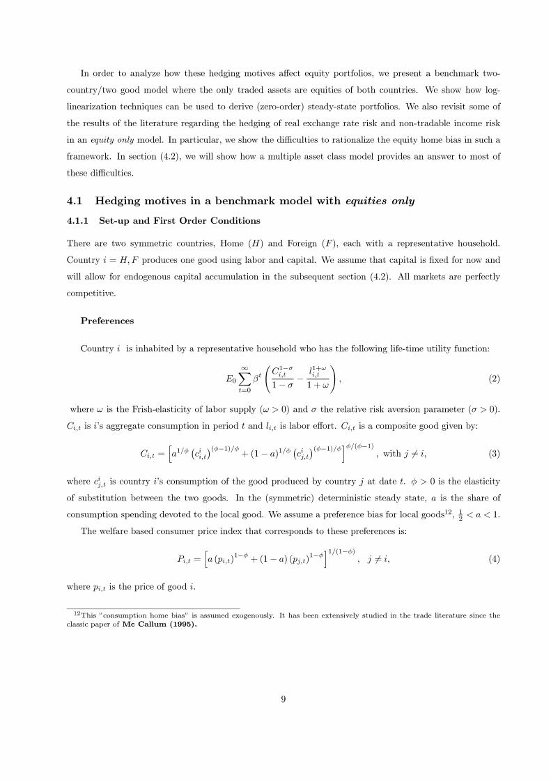
In order to analyze how these hedging motives affect equity portfolios, we present a benchmark two-

country/two good model where the only traded assets are equities of both countries. We show how log-

linearization techniques can be used to derive (zero-order) steady-state portfolios. We also revisit some of

the results of the literature regarding the hedging of real exchange rate risk and non-tradable income risk

in an equity only model. In particular, we show the difficulties to rationalize the equity home bias in such a

framework. In section (4.2), we will show how a multiple asset class model provides an answer to most of

these difficulties.

4.1 Hedging motives in a benchmark model with equities only

4.1.1 Set-up and First Order Conditions

There are two symmetric countries, Home (H) and Foreign (F ), each with a representative household.

Country i = H,F produces one good using labor and capital. We assume that capital is fixed for now and

will allow for endogenous capital accumulation in the subsequent section (4.2). All markets are perfectly

competitive.

Preferences

Country i is inhabited by a representative household who has the following life-time utility function:

E0

∞∑

t=0

βt(C1−σi,t

1− σ−

l1+ωi,t

1 + ω

), (2)

where ω is the Frish-elasticity of labor supply (ω > 0) and σ the relative risk aversion parameter (σ > 0).

Ci,t is i’s aggregate consumption in period t and li,t is labor effort. Ci,t is a composite good given by:

Ci,t =[a1/φ

(cii,t

)(φ−1)/φ+ (1− a)1/φ

(cij,t

)(φ−1)/φ]φ/(φ−1)

, with j �= i, (3)

where cij,t is country i’s consumption of the good produced by country j at date t. φ > 0 is the elasticity

of substitution between the two goods. In the (symmetric) deterministic steady state, a is the share of

consumption spending devoted to the local good. We assume a preference bias for local goods12, 12 < a < 1.

The welfare based consumer price index that corresponds to these preferences is:

Pi,t =[a (pi,t)

1−φ + (1− a) (pj,t)1−φ

]1/(1−φ), j �= i, (4)

where pi,t is the price of good i.

12This ”consumption home bias” is assumed exogenously. It has been extensively studied in the trade literature since theclassic paper of Mc Callum (1995).

9

Technologies and firms’ decisions

In period t, country produces yi,t units of good i according to the production function

yi,t = θi,t (k0)α (li,t)

1−α, (5)

with 0 < α < 1. k0 is the country’s initial stock of capital. It is fixed. Total factor productivity (TFP)

θi,t > 0 is an exogenous random variable.

There is a (representative) firm in country i that hires local labor and produces output, using technology

(5). Due to the Cobb-Douglas technology, a share 1−α of output at market prices is paid to workers. Thus,

the country i wage incomes are:

wi,tli,t = (1− α)pi,tyi,t (6)

where wi,t is the country i wage rate.

A share α of country i output at market prices is paid as a dividend di,t to shareholders:

di,t = αpi,tyi,t (7)

Financial markets and instantaneous budget constraint

Financial markets are frictionless. There is international trade in stocks. The country i representative

firm issues a stock that represents a claim to its stream of dividends {di,t}. The supply of shares is normalized

at unity. Each household fully owns the local stock, at birth, and has zero initial foreign assets. Let Sij,t+1

denote the number of shares of stock j held by country i at the end of period t. At date t, the country i

household faces the following budget constraint:

Pi,tCi,t + pSi,tSii,t+1 + pSj,tS

ij,t+1 = wi,tli,t + (di,t + pSi,t)S

ii,t + (dj,t + pSj,t)S

ij,t, j �= i, (8)

where pSi,t is the price of stock i.

Household decisions and market clearing conditions

Each household selects portfolios, consumptions and labor supplies that maximize her life-time utility

(2) subject to her budget constraint (8) for t ≥ 0. The following equations are first-order conditions of that

decision problem:

cii,t = a

(pi,tPi,t

)−φ

Ci,t, cij,t = (1− a)

(pj,tPi,t

)−φ

Ci,t, lωi,t =

(wi,tPi,t

)Ci,t

−σ (9)

1 = Et

[β

(Ci,t+1

Ci,t

)−σ

Pi,tPi,t+1

pSj,t+1 + dj,t+1

pSj,t

]for j = H,F . (10)

(9) represents the optimal allocation of consumption spending across goods, and the labor supply decision.

(10) shows the Euler equations with respect to the two stocks.

10

Market-clearing in goods and asset markets requires:

cHH,t + cFH,t = yH,t , cFF,t + cHF,t = yF,t , (11)

SHH,t + SFH,t = SFF,t + SHF,t = 1 (12)

4.1.2 Zero-order equilibrium portfolios

Equilibrium portfolio holdings chosen at date t (Sii,t+1, Sij,t+1) are functions of state variables at date

t. Devereux and Sutherland (2008a) show how to compute Taylor expansion of the portfolio decision

rules, in the neighborhood of the deterministic steady state. In this Section, we provide closed form solutions

for ‘zero-order portfolios’ (denoted by variables without time subscripts) Sii , Sij , i.e. portfolio decision rules

evaluated at steady state values of state variables. These portfolios can be determined by linearizing the

model around its deterministic steady state. We show that the asset structure (two assets with two exogenous

shocks) is “locally-complete” in the sense that up to a first order linear approximation, the consumption

allocation is efficient (in other words there is perfect risk sharing up to a first-order approximation of the

model). The method we use to solve for portfolios is then slightly different fromDevereux and Sutherland

(2008a) as it does not require a second-order expansion of the Euler equations (equation ((10)). We simply

derive the portfolio that replicates the efficient allocation up to a first-order approximation of the non-

portfolio equations. This method is simpler but less general than Devereux and Sutherland (2008a) as

theirs can also be applied in models with incomplete financial markets.

Log-linearization of the model

In what follows, zt ≡zH,t

zF,tdenotes the ratio of Home over Foreign variables; zt ≡ (zt − z)/z denotes the

relative deviation of a variable zt from its steady state value z.

The Home country’s CPI-based real exchange is RERt ≡PH,t

PF,t. Linearizing this expression gives (using

(4)):

RERt = PH,t − PF,t = (2a− 1) qt. (13)

where qt ≡ pH,t/pF,t denotes the country H terms of trade. Due to consumption home bias (a > 12), an

improvement of Home terms of trade generates an appreciation of the Home real exchange rate (without

home bias in consumption, the real exchange rate is constant).

In an equilibrium with “locally-complete” markets, the ratio of Home and Foreign marginal utilities of

aggregate consumption is proportional to the consumption-based real exchange rate (Backus and Smith

(1993), Kollmann (1995)). Linearization of this risk sharing condition gives:

−σ(CH,t − CF,t) = (2a− 1) qt. (14)

Using intratemporal first-order condition for consumption (9) and market-clearing condition (11), one

can show that when (14) holds, relative world consumption demand is given by yt = yH,t/yF,t ≡ (cHH,t +

11

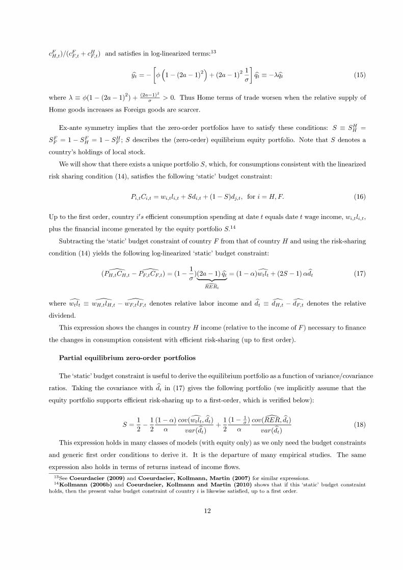
cFH,t)/(cFF,t + cHF,t) and satisfies in log-linearized terms:

13

yt = −

[φ(1− (2a− 1)2

)+ (2a− 1)2

1

σ

]qt ≡ −λqt (15)

where λ ≡ φ(1 − (2a− 1)2) + (2a−1)2

σ > 0. Thus Home terms of trade worsen when the relative supply of

Home goods increases as Foreign goods are scarcer.

Ex-ante symmetry implies that the zero-order portfolios have to satisfy these conditions: S ≡ SHH =

SFF = 1 − SFH = 1 − SHF ; S describes the (zero-order) equilibrium equity portfolio. Note that S denotes a

country’s holdings of local stock.

We will show that there exists a unique portfolio S, which, for consumptions consistent with the linearized

risk sharing condition (14), satisfies the following ‘static’ budget constraint:

Pi,tCi,t = wi,tli,t + Sdi,t + (1− S)dj,t, for i = H,F. (16)

Up to the first order, country i′s efficient consumption spending at date t equals date t wage income, wi,tli,t,

plus the financial income generated by the equity portfolio S.14

Subtracting the ‘static’ budget constraint of country F from that of country H and using the risk-sharing

condition (14) yields the following log-linearized ‘static’ budget constraint:

( PH,tCH,t − PF,tCF,t) = (1−1

σ)(2a− 1) qt︸ ︷︷ ︸

RERt

= (1− α)wtlt + (2S − 1)αdt (17)

where wtlt ≡ wH,tlH,t − wF,tlF,t denotes relative labor income and dt ≡ dH,t − dF,t denotes the relative

dividend.

This expression shows the changes in country H income (relative to the income of F ) necessary to finance

the changes in consumption consistent with efficient risk-sharing (up to first order).

Partial equilibrium zero-order portfolios

The ‘static’ budget constraint is useful to derive the equilibrium portfolio as a function of variance/covariance

ratios. Taking the covariance with dt in (17) gives the following portfolio (we implicitly assume that the

equity portfolio supports efficient risk-sharing up to a first-order, which is verified below):

S =1

2−1

2

(1− α)

α

cov(wtlt, dt)

var(dt)+1

2

(1− 1σ )

α

cov(RER, dt)

var(dt)(18)

This expression holds in many classes of models (with equity only) as we only need the budget constraints

and generic first order conditions to derive it. It is the departure of many empirical studies. The same

expression also holds in terms of returns instead of income flows.

13See Coeurdacier (2009) and Coeurdacier, Kollmann, Martin (2007) for similar expressions.14Kollmann (2006b) and Coeurdacier, Kollmann and Martin (2010) shows that if this ‘static’ budget constraint

holds, then the present value budget constraint of country i is likewise satisfied, up to a first order.

12

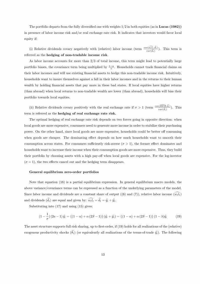
The portfolio departs from the fully diversified one with weights 1/2 in both equities (as in Lucas (1982))

in presence of labor income risk and/or real exchange rate risk. It indicates that investors would favor local

equity if:

(i) Relative dividends covary negatively with (relative) labor income (term cov(wtlt,dt)

var(dt)). This term is

referred as the hedging of non-tradable income risk.

As labor income accounts for more than 2/3 of total income, this term might lead to potentially large

portfolio biases, the covariance term being multiplied by 1−αα . Households cannot trade financial claims on

their labor incomes and will use existing financial assets to hedge this non-tradable income risk. Intuitively,

households want to insure themselves against a fall in their labor incomes and in the returns to their human

wealth by holding financial assets that pay more in these bad states. If local equities have higher returns

(than abroad) when local returns to non-tradable wealth are lower (than abroad), households will bias their

portfolio towards local equities.

(ii) Relative dividends covary positively with the real exchange rate if σ > 1 (term cov(RER,dt)

var(dt)). This

term is referred as the hedging of real exchange rate risk.

The optimal hedging of real exchange rate risk depends on two forces going in opposite direction: when

local goods are more expensive, consumers need to generate more income in order to stabilize their purchasing

power. On the other hand, since local goods are more expensive, households could be better off consuming

when goods are cheaper. The dominating effect depends on how much households want to smooth their

consumption across states. For consumers sufficiently risk-averse (σ > 1), the former effect dominates and

households want to increase their income when their consumption goods are more expensive. Thus, they build

their portfolio by choosing assets with a high pay-off when local goods are expensive. For the log-investor

(σ = 1), the two effects cancel out and the hedging term disappears.

General equilibrium zero-order portfolios

Note that equation (18) is a partial equilibrium expression. In general equilibrium macro models, the

above variance/covariance terms can be expressed as a function of the underlying parameters of the model.

Since labor income and dividends are a constant share of output ((6) and (7)), relative labor income (wtlt)

and dividends (dt) are equal and given by: wtlt = dt = qt + yt.

Substituting into (17) and using (15) gives:

(1−1

σ) (2a− 1) qt = {(1− α) + α (2S − 1)} (qt + yt) = {(1− α) + α (2S − 1)} (1− λ)qt (19)

The asset structure supports full risk sharing, up to first-order, if (19) holds for all realizations of the (relative)

exogenous productivity shocks (θt) (or equivalently all realizations of the terms-of-trade qt). The following

13

portfolio S ensures that (19) holds for arbitrary realizations of qt:

S =1

2−1

2

(1− α)

α−1

2(1−

1

σ)(2a− 1)

α (λ− 1)(20)

The equilibrium portfolio is the sum of three terms:

(i) The first term 12 is a pure diversification term. It would prevail if there were no hedging motives as in

Lucas (1982). In the absence of heterogeneity across investors, there is full diversification of national

output risk. We derive the Lucas portfolio when α→ 1 (no human capital risk) and when a = 1/2 (no

real exchange rate risk).

(ii) The second term −12(1−α)α is the hedging of non-tradable income risk (as in Baxter and Jermann

(1997)): changes in output driven by productivity shocks are shared in constant proportion (Cobb-

Douglas production). This leads to a perfect correlation between labor incomes and capital incomes:

households should short the local stock to hedge human capital risk. Note that in the present model,

the portfolio is exactly the one of Baxter and Jermann (1997) in the absence of real exchange rate

risk (a = 1/2).

(iii) The third term −12(1 −

1σ )

(2a−1)α(λ−1) is the hedging of real exchange rate risk. This term is the same as

the one derived in Coeurdacier (2009) and Kollmann (2006b) in the absence of human capital

risk (α → 1). This term cancels out for a log-investor (σ = 1). As explained above (see equation

(18)), investors bias their portfolio towards equities that have high returns when local goods are more

expensive (if σ > 1). The appropriate portfolio depends on the value of λ i.e on the elasticity of

substitution φ. Three different cases emerge:

(a) λ > 1 (i.e. an elasticity of substitution φ roughly above unity): the hedging of real exchange rate

risk generates a Foreign equity bias. The reason is the following: a (relative) fall in local output

driven by a bad productivity shock triggers a moderate increase in the Home terms-of-trade, a

moderate appreciation of the Home real exchange rate together with a decrease in Home equity

returns: Foreign equities are more valuable since they have higher (relative) returns despite the

Home real exchange rate appreciation.

(b) λ < 1 (i.e. elasticity of substitution φ, roughly below unity): a (relative) fall in local output

triggers a stronger improvement of the Home terms-of-trade and a stronger appreciation of the

Home real exchange rate. As the relative price response is stronger, Home equity excess returns

increase. Home investors exhibit Home equity bias as Home equity have higher returns when the

Home real exchange rate appreciates. This is the case emphasized by Kollmann (2006b).

(c) λ = 1: Any increase in local output is perfectly offset by a fall in the terms-of-trade. Both

equities are perfect substitutes and there is portfolio indeterminacy. This is an extension of Cole

and Obstfeld (1991)’s result.

14

4.1.3 Related literature

Hedging real exchange rate risk

As appears clearly in the previous model, optimal portfolios are structured to hedge the risk arising from

real exchange rate fluctuations. This is at the heart of the potential divergence of portfolios across investors

in the partial equilibrium portfolio choice models with real exchange rate risk. The key issue is whether

local equities are a good hedge against relative price (real exchange rate) fluctuations, i.e. whether local

equities have higher returns when local goods are (relatively) more expensive. If this is the case, then local

investors should favor local equities. Early examples of this hypothesis are Solnik (1974), Adler and

Dumas (1983), Krugman (1981), de Macedo (1983), de Macedo et al. (1985) and Stulz (1981).

Cooper and Kaplanis (1994) start with the premise that for equity home bias to be rooted in a desire to

hedge against relative inflation, equity returns need to be positively correlated with inflation. They test for

such a correlation and reject it for all countries considered. These early papers take relative prices (and the

real exchange rate) and asset returns as given while in the present model and, more generally in the recent

Open Economy Financial Macroeconomics, the dynamics of goods prices and asset returns is endogenous,

as is the covariance between the two.

In the more recent literature, some contributions focus on the hedging of the relative price of tradables

(terms-of-trade, as in the present model) and some focus on the hedging of the relative price of non-tradable

goods. In their influential contribution, Obstfeld and Rogoff (2000) argue that trade costs in goods

markets help to solve the equity home bias puzzle. The above model (in line with Coeurdacier (2009))15

shows the opposite result for most parameter values (in particular for φ and σ above unity). Indeed, in

Obstfeld and Rogoff (2000), the coefficient of risk aversion is below unity (and equal to the inverse of

the elasticity of substitution between the two goods), which allows to solve the model in closed-form. With

such preferences, agents prefer to hold local equities which pay less when local consumption is expensive. A

similar point is made by Uppal (1993) in a two country/one good model in continuous time with trade

costs: he shows that home bias only arises for the coefficient of relative risk aversion smaller than one. One

can potentially restore the argument of Obstfeld and Rogoff (2000) in the present model if σ is above 1

but the elasticity of substitution between goods φ is below unity. In that case, a fall in Home supply triggers

a very large increase in the Home terms-of-trade such that Home equity returns are high when prices of Home

goods are high. Hence, investors would rather hold local equities (see Kollmann (2006b)). In this class of

models, equity home bias relies on the response of relative prices, i.e. on the elasticity of substitution between

local and foreign products. While time series macro data estimating the response of trade to exchange rate

changes suggests a low elasticity of substitution, between 0.5 and 1.5 (see Hooper and Marques (1995),

Backus, Kehoe and Kydland (1994) and Heathcote and Perri (2002)), bilateral sectoral trade data

suggests a large elasticity, -above 5 for most sectors (see Harrigan (1993), Hummels (2001) and Baier

15The model presented features home bias in preferences instead of trade costs. A functional transformation of trade costswould however make the two types of models isomorphic.

15

and Bergstrand (2001) among others)-.16 The parameter uncertainty makes it hard to get a conclusive

answer from this class of models. It is also important to note that output fluctuations in all these classes

of models are driven by supply shocks. In the presence of demand shocks, equilibrium portfolios could turn

out to be different: when local demand is high, both prices of local goods and payoffs of local firms increase.

Hence, demand shocks can generate positive co-movements between local equity returns and the price of

local goods (see Pavlova and Rigobon (2007)). In order to be able to consume when demand is high,

local investors would prefer local equities.

Similarly, the presence of nontradable consumption exposes domestic agents to real exchange rate risk

(driven by fluctuations in the relative price of non-tradable goods). Stockman and Dellas (1989) develops

a two country model with endowment economies. Each country has random endowments of a (single) traded

good and a nontraded good. There is trade in equities of tradable and nontradable goods firm. With utility

separable in tradable and nontradable consumption, optimal portfolios imply that domestic agents hold all of

the equity of domestic nontradable firms. By holding all of the equity of nontraded goods, domestic agents

hold an asset whose return is perfectly correlated with their expenditure on nontraded goods. Domestic

agents hold the same share of Home and Foreign equity of tradable firms, implying perfect diversification

in the tradable sector as in Lucas (1982). Thus, this model generates home bias in equity positions,

and the home bias increases in the share of nontradable consumption in total output. Various papers have

extended this framework to more general preferences, investigating in particular the non-separability between

tradable and non-tradable consumption together with multiple tradable goods (see Baxter et al (1998),

Serrat (2001),17 Obstfeld (2007), Matsumoto (2007), Collard et al. (2007)).18 In these papers,

the presence of nontradable consumption interacts with tradable consumption and some degree of home

bias in nontradable equities obtains. The precise structure of portfolios is strongly dependent on preference

parameters, in particular the substitution elasticities between tradable and nontradable goods (and also

between domestic and foreign tradable goods). The mechanism at the heart of the home bias towards non-

tradable equity is however essentially similar to the one described in the previous model: investors want

to hold equities whose payoff is high when the real exchange rate appreciates, i.e when the consumption of

non-tradable goods is expensive. It turns out that for a sufficiently low elasticity of substitution between

tradable and nontradable goods (roughly below unity as found in the empirical literature),19 a fall in local

non-tradable output implies a strong increase in the relative price of non-tradable goods together with an

16Imbs and Mejean (2009) claims that the discrepancy between macro and micro estimates comes from an aggregationbias; correcting for this bias, they find an elasticity of up to 7.

17See also Kollmann (2006a) for a comment.18In earlier work, Eldor et al. (1988) in a general equilibrium model studies n countries, each producing a nontradable

good and the single tradable good that is consumed in all countries. The assets traded are ”real equities” for the tradableand nontradable good. Tradable equities pay one unit of the traded good in each state of the world, while nontradable equitypays out θ units of the nontradable good, where θ is state contingent nontradable output. They point out that for home biasto arise the returns of nontraded equities have to be positively correlated with the price of the nontradable good and deriveconditions for the risk aversion parameter, the price elasticity of demand for tradable goods and the income elasticity of demandfor tradable goods such that it would be the case.

19Typical values used for the elasticity of substitution between tradable and non-tradable goods are: 0.44 (Stockman andTesar (1995)), 0.74 (Mendoza (1995)), from 0.6 to 0.8 (Serrat (2001)). Ostry and Reinhart (1992) provides estimatesfor developing countries in the range of 0.6 to 1.4. SeeMatsumoto (2007) for a more detailed discussion.

16

increase in local non-tradable equity returns: hence, local non-tradable equity returns comove positively with

the price of non-tradable goods (and the real exchange rate), leading to local equity bias in that sector.

On the empirical front, Pesenti and van Wincoop (2002) derive an expression that relates home

bias to the correlation between equity returns and nontradable consumption growth20 and using data on 14

OECD countries from 1970 to 1993, they find that, on average, nontradable consumption growth is positively

correlated with the return on domestic capital. This would imply that home bias would arise if tradables

and nontradable goods are complementary. The authors find, however, that even in those cases, hedging

nontradable consumption could at best explain a relatively small fraction of the home bias observed in the

data. Overall, there are two empirical difficulties with an explanation of the equity home bias relying on

the presence of a non-tradable sector. The first one is that the structure of portfolios is strongly dependent

on preference parameters, which are not easy to estimate. The second one is that the home bias result

relies on the ability of investors to hold separate claims on tradable and non-tradable output: as most

products contain both tradable and non-tradable components, shares of firms automatically involve joint

claims on tradables and non-tradables. This difficulty is made all the more relevant by the fact that, when

agents are allowed to trade separate claims on tradable and non-tradable output, optimal equity positions

are very different across the two sectors. This different structure of portfolios across traded and non-traded

sectors seems “inconsistent with casual empiricism” as argued by Lewis (1999). More broadly, empirical

analysis of this channel is also hindered by the difficulty to identify precisely nontradable consumption and

tradable/nontradable equity.

There is yet another major empirical issue faced by this explanation of home bias. The hedging of real

exchange rate risk leads to equity home bias if local equities have higher returns (than abroad) when local

prices are higher (than abroad). In other words, equity home bias appears if excess local equity returns

(over foreign) increase when the real exchange rate appreciates (the term cov(RER,dt)

var(dt)in equation (18)). As

shown by van Wincoop and Warnock (2008), the empirical correlation between excess equity returns

and the real exchange rate is very low, too low to explain observed equity home bias. Furthermore, most of

the fluctuations in the real exchange rate represent fluctuations in the nominal exchange rate: as explained

in section (4.2), these could be hedged using positions in the forward currency market or the currency bond

market. In other words, equities do not seem empirically to be an appropriate asset to insure investors

against real exchange rate fluctuations. Hence, while these models are theoretically appealing, it is doubtful

that the hedging of real exchange rate risk can account empirically for the equity home bias.

Hedging non-tradable income risk

In our model (see equation (18)), hedging non-tradable income risk implies picking stocks which have

higher payoffs when labour income is low. The focus of the literature has been twofold: first, from a

theoretical perspective, it has discussed the conditions under which standard macroeconomic models imply

a negative or positive correlation between local equity returns and returns to non-tradable wealth. Second,

20Their model also includes leisure which drives another hedging motive.

17

from an empirical perspective, a series of papers have provided estimates of the covariance between relative

equity returns and relative returns to human wealth which is the key empirical counterpart of portfolio biases

in this class of models.

The most influential contribution on these matters is Baxter and Jermann (1997), who argue that the

presence of non-tradable income risk worsens the equity home bias puzzle. Their argument goes as follows:

in a standard multi-country real business cycle model with a single tradable good and a Cobb-Douglas

production function, changes in output are shared in constant proportion between capital and labor. Hence,

labor and capital incomes are perfectly correlated. As investors are already strongly exposed to domestic risk

due to their labor income, they should not hold local capital. Due to the relatively large labour share in all

countries, the effects of hedging domestic human capital dominates the benefits of diversification: investors

should short-sell local equities (term −121−αα in equation (20)). Hence, the equity home bias puzzle is worse

than we think! The authors estimate a vector error correction model that allows the correlation between

labour and capital returns to vary over time and be imperfect, while maintaining the assumption that the

ratio of labour to capital income is stationary. Using data from the OECD National Accounts (1994) for

Japan, UK, Germany, and US for 1960-1993, they find that within countries, labour and capital returns

are highly correlated, while the correlation between domestic labour returns and foreign equity returns is

quite low. Using the observed correlations, the authors then construct diversified portfolios and find that

the optimal position in domestic equity is negative in all the countries considered.

Their empirical findings have been challenged by a series of papers : Bottazzi et al (1996) use a

continuous time VAR model of portfolio choice and data on a large set of OECD countries and find that

returns to domestic capital and human capital are negatively correlated for most countries but the US and

this can explain a fraction of equity home bias in these countries. Julliard (2002) argues that the Baxter

and Jermann (1997)’s empirical findings are due to an econometric misspecification : the correlation

between returns to human capital and local equity returns is overstated because they implicitly assume

that innovations to capital and labor incomes are independent across countries. Once the misspecification

is corrected, considering human capital risk does not unequivocally worsen the home bias puzzle. Using

micro-level data, Massa and Simonov (2006) show that non-financial income is uncorrelated with the

market portfolio of financial assets, but actual investors’ portfolios (which differ from the market portfolio)

are more positively correlated with non-financial income than the market portfolio is. Thus, the authors cast

doubt on the rationality of investors and on their desire to hedge non-tradable income risk.

From a theoretical perspective, Heathcote and Perri (2008) shows that Baxter and Jermann

(1997)’s result relies on very strong assumptions: one single and perfectly tradable good and a fixed capital

stock. Relaxing those assumptions (in a two-country/two-good international real business cycle model a la

Backus, Kehoe and Kydland (1994)) and introducing differentiated product across countries together

with consumption/investment home bias changes drastically the picture and helps solve the equity home bias

puzzle. Their result relies on two key elements: endogenous capital accumulation and a strong adjustment

18

of relative prices.21 The main intuition is the following. Suppose a positive (persistent) productivity shock

hits the Home economy. This leads to:

(i) a fall in the relative price of Home goods (Foreign goods are scarcer).

(ii) an increase in Home investment (more than abroad) as Home investment uses more intensively cheaper

Home goods (due to home bias in investment spending).

(iii) an increase in Home wages (more than abroad) and in the Home returns to non-tradable wealth.

(iv) a decrease in the returns on Home capital (relative to Foreign) if the (relative) price response of

Home goods is strong enough.

The main difference with Baxter and Jermann (1997) is the last point (iv): if the market price of

Home goods falls sufficiently and Home investment is increasing, dividends distributed by Home firms (which

are net of investment) are lower than abroad, and so are Home returns to capital. Hence the model generates

negative co-movements between Home (excess) returns to human wealth and Home (excess) returns to capital:

hedging non-tradable income risk implies home equity bias. Home bias in investment/consumption spending

is important as it triggers a stronger response of investment at Home, thus a larger fall of Home dividends

and a larger increase of Home wages. Importantly, the model generates a positive link between consumption

home bias and equity home bias as found in the data.22 Note that Heathcote and Perri (2008) focus

on log-utility and unitary elasticity of substitution between Home and Foreign goods. Increasing the level

of risk aversion introduces a real exchange rate risk motive as in Coeurdacier (2009) and Kollmann

(2006b). Increasing the elasticity of substitution reduces the response of relative prices and makes the

portfolio converge towards the one of Baxter and Jermann (1997).

4.2 Hedging motives in a benchmark model with multiple asset classes (bonds

and equities)

4.2.1 Hedging with bond and equities: the role of ”conditional risk”

The first generation of papers presented above focus on equity positions to rationalize home bias. However,

equities are only part of financial assets traded internationally. Debt securities (nominal bonds in different

currencies, corporate bonds, bank deposits,...) are instruments that can also be used to share risks inter-

nationally (see section (7)). They should not be excluded from our models, first for realism, since they

constitute a large share of international asset flows but above all because there might be substitution across

asset classes. Hence, equity positions derived in equity only models might be sensitive to the presence of

other financial assets. Recent models with portfolio decisions have incorporated multiple assets (equities and

bonds) to have more robust and realistic predictions.23 Nominal bond returns differentials across countries

21Endogenous capital accumulation is crucial: despite multiple goods, Baxter and Jermann (1997)’s results would surviveif capital is fixed.

22Lane (2000), Aizenman and Noy (2004), Heathcote and Perri (2008) among others show a positive relationshipbetween trade openness and foreign equity holdings looking at a cross section of countries. Portes and Rey (2005), Aviatand Coeurdacier (2007) and Lane and Milesi-Feretti (2008) show that country equity portfolios are strongly biasedtowards trading partners.

23As described in section (4.2.5), recent contributions with multiple asset classes include Engel and Matsumoto (2008a,b),Coeurdacier, Kollmann andMartin (2007 and 2010), Coeurdacier and Gourinchas (2010), Berriel and Bhattarai

19

are (almost) perfectly correlated with the real exchange rate (in developed countries, fluctuations in the nom-

inal exchange rate account for most of the fluctuations in the real exchange rate). Hence, bonds are better

suited than equities to hedge real exchange rate risk. But this is not the end of the story. The presence of

bonds also affects the hedging properties of equities for non-tradable income risk. Equities are used to hedge

sources of risks that cannot be hedged through the bond positions, in particular the part of non-tradable

income risk that is orthogonal to bond returns. In this new literature, the optimal equity position depends

therefore on the correlation of returns on equity with returns on non-tradable income, conditional on bond

returns.

4.2.2 Set-up of the Model

We use a similar set up as in section (4.1) but we add two important ingredients to formalize our above

discussion on hedging motives: endogenous capital accumulation and trade in real bonds. They allow us to

overcome the limitations of the model presented in (4.1): first, endogenous investment in a two-good model

breaks the perfect link between returns on physical capital and returns on human capital; second, bond

trading modifies the hedging properties of equities. Bonds will be used to hedge fluctuations in the real

exchange rate. Equities will be used to hedge non-tradable income risk, conditionally on bond returns.

This model is similarCoeurdacier, Kollmann and Martin (2010) which extendsHeathcote and Perri

(2008) to multiple asset classes (bonds and equities).

In presence of productivity shocks only, we would face a portfolio indeterminacy in a first-order ap-

proximation of the non-portfolio equations since the number of available assets (bonds and equities in each

country) would exceed the exogenous sources of uncertainty. We have to add an additional source of uncer-

tainty. We choose to add shocks to the disutility of leisure for simplicity. As explained in Coeurdacier,

Kollmann and Martin (2010) and Coeurdacier and Gourinchas (2010), the nature of the additional

shock used to alleviate portfolio indeterminacy is irrelevant for the portfolio and results would survive with

other shocks commonly used (shocks to investment a la Greenwood, Hercowitz and Huffman (1988),

depreciation shocks, shocks to capacity utilization...).24

Hence, preferences are now defined by:

E0

∞∑

t=0

βt(C1−σi,t

1− σ− χi,t

l1+ωi,t

1 + ω

), (21)

where χi,t is an exogenous shock to the disutility of labor.

Technologies and capital accumulation

As before, production in each country uses capital and labor with a Cobb-Douglas production function:

yi,t = θi,t (ki,t)α(li,t)

1−α, (22)

(2008), Devereux and Sutherland (2007 and 2008b).24Obviously, a different shock will have different business cycles implications but we are presently not interested in those.

20

The law of motion of the capital stock is:

ki,t+1 = (1− δ)ki,t + Ii,t (23)

where 0 < δ < 1 is the depreciation rate of capital. Ii,t is gross investment in country i at date t. In both

countries, gross investment is generated using Home and Foreign inputs:

Ii,t =[a1/φ

(iii,t

)(φ−1)/φ+ (1− a)1/φ

(iij,t

)(φ−1)/φ]φ/(φ−1)

, j �= i, (24)

where iij,t is the amount of good j used for investment in country i. We assume local bias for investment

spending (identical to the one for consumption),25 12 < a < 1. The associated investment price index is the

same as for consumption Pi,t (see equation (4)).

Firms’ decisions

A share 1 − α of output at market prices is paid to workers as in equation (6). A share α of country i

output, net of physical investment spending is paid as a dividend di,t to shareholders:

di,t = αpi,tyi,t − Pi,tIi,t (25)

The firm chose Ii,t to equate the expected future marginal gain of investment to the marginal cost. This

implies the following first-order condition:26

Pi,t = βEt[(Ci,t+1/Ci,t)

−σ(Pi,t/Pi,t+1)[pi,t+1θi,t+1αkα−1i,t+1l

1−αi,t+1 + (1− δ)Pi,t+1]

], (26)

The firm chooses the Home and Foreign investment inputs iii,t, iij,t that minimize the cost of generating Ii,t.

This leads to the following intratemporal allocation for investment goods:

iii,t = a

(pi,tP Ii,t

)−φ

Ii,t, iij,t = (1− a)

(pj,tPi,t

)−φ

Ii,t, j �= i. (27)

Financial markets and instantaneous budget constraint:

There is now international trade in stocks and (real) bonds. Stocks in country i represents a claim to

its stream of dividends {di,t}. There is a bond denominated in the Home good, and a bond denominated

in the Foreign good. Buying one unit of the Home (Foreign) bond in period t gives one unit of the Home

(Foreign) good in all future periods. Both bonds are in zero net supply. We denote by Sij,t+1 the number of

shares of stock j held by country i at the end of period t, while Bij,t+1 represents claims held by country i

25See Coeurdacier, Kollmann and Martin (2009) and Castello (2009) for a model where bias in investment spendingis different from the bias in consumption spending.

26Note that we use the intertemporal marginal rate of substitution of the country i household for investment decisions incountry i. This assumption is however irrelevant here since up-to the degree of the approximation, the intertemporal marginalrate of substitution of the country i household and the country j household are the same.

21

(at the end of t) to future unconditional payments of good j. At date t, the country i household now faces

the following budget constraint:

Pi,tCi,t + pSi,tSii,t+1 + pSj,tS

ij,t+1 + pBj,tB

ij,t+1 + pBi,tB

ii,t+1 (28)

= wi,tli,t + (di,t + pSi,t)Sii,t + (dj,t + pSi,t)S

ij,t + (pi,t + pBi,t)B

ii,t + (pj,t + pBj,t)B

ij,t, j �= i,

where pSi,t is the price of stock i and pBi,t is the price of bond i.

Household decisions and market clearing conditions

Households’ first-order conditions for that decision problem are still given by (9) and (10). One needs to

add the Euler equations for the two bonds:

1 = Etβ

(Ci,t+1

Ci,t

)−σ

Pi,tPi,t+1

pBj,t+1 + pj,t+1

pBj,tfor j = H,F . (29)

Market-clearing in goods and asset markets now requires:

cHH,t + cFH,t + iHH,t + iFH,t = yH,t , cFF,t + cHF,t + iFF,t + iHF,t = yF,t , (30)

SHH,t + SFH,t = SFF,t + SHF,t = 1, (31)

BHH,t +BF

H,t = BFF,t +BH

F,t = 0.

4.2.3 Zero-order equilibrium portfolios

As in section (4.1), equilibrium portfolio holdings (Sii,t+1, Sij,t+1,B

ii,t+1, B

ij,t+1) can be determined by lin-

earizing the model around its deterministic steady state. With the asset structure here (four assets with four

exogenous shocks), efficient risk sharing can be replicated up to the first-order (“locally-complete” markets).

Linearization of the model

We use the same notation as in section (4.1). Equations (13) and (14) still hold.

Linearization of the relative demand for investment yI,t ≡iHH,t+i

FH,t

iFF,t

+iHF,t

gives (using the intratemporal allo-

cation across investment goods (27)):

yI,t = −φ(1− (2aI − 1)

2)qt + (2a− 1)It, (32)

where It ≡ IH,t/IF,t is relative real aggregate investment. Holding constant the terms of trade, the relative

demand for Home investment goods, yI,t, increases with relative real investment in the Home country, It,

since Home aggregate investment is biased towards the Home good (a > 12).

22

The relative demand for consumption yC,t is still defined by (from (15)):

yC,t = −

[φ(1− (2a− 1)2

)+ (2a− 1)2

1

σ

]qt ≡ −λqt (33)

The market clearing condition for goods (30), together with (32) and (33) implies:

(1− sI)yC,t + sI yI,t = −µqt + sI(2aI − 1)It = yt (34)

where µ = φ(1−(2a− 1)2)+(1−sI)(2a−1)2

σ > 0 and sI ≡P I

HIHpHyH

= P IF IF

pF yFis the steady state investment/GDP

ratio.

Not surprisingly, Home terms of trade worsen when the relative supply of Home goods increases, for a

given amount of relative Home country investment. Home terms of trade improve when Home investment

rises (due to home bias in investment spending), for a given value of the relative Home/Foreign output.

Ex-ante symmetry implies that the zero-order portfolios have to satisfy the following conditions: S ≡

SHH = SFF = 1 − SFH = 1 − SHF ; B ≡ BHH = BF

F = −BFH = −BH

F . The pair (S;B) thus describes the

(zero-order) equilibrium portfolio. B denotes a country holdings of bonds denominated in its local good.

B > 0 means that a country is long in local-good bonds (and short in foreign good bonds).

As before there exists a unique portfolio (S;B) that satisfies the following ‘static’ budget constraint, for

consumptions that are consistent with the linearized risk sharing condition (14):

Pi,tCi,t = wi,tli,t + Sdi,t + (1− S)dj,t +B(pi,t − pj,t), for i = H,F. (35)

Country i′s efficient consumption spending at date t equals date t wage income, wi,tli,t, plus the financial

income generated by the portfolio (S;B)

Subtracting the ‘static’ budget constraint of country F from that of country H and linearizing gives:27

(1− sI)( PH,tCH,t − PF,tCF,t) = (1− sI)(1−1

σ)(2a− 1) qt︸ ︷︷ ︸

RERt

= (1− α)wtlt + (2S − 1) (α− sI)dt + 2bqt (36)

where b = By denotes holdings of debt denominated in local good, divided by steady-state GDP.

Partial equilibrium zero-order portfolios

Like in the previous model, one can derive from the ‘static’ budget constraint (36) a partial equilibrium

portfolio that expresses the hedging terms in terms of covariance-variance ratios. This expression holds in a

large class of models with bonds and equities.

Projection of (36) on dt and qt gives the following expression for the portfolio of bonds and equities (S,

27We assume α > sI to have strictly positive dividends in the steady-state.

23

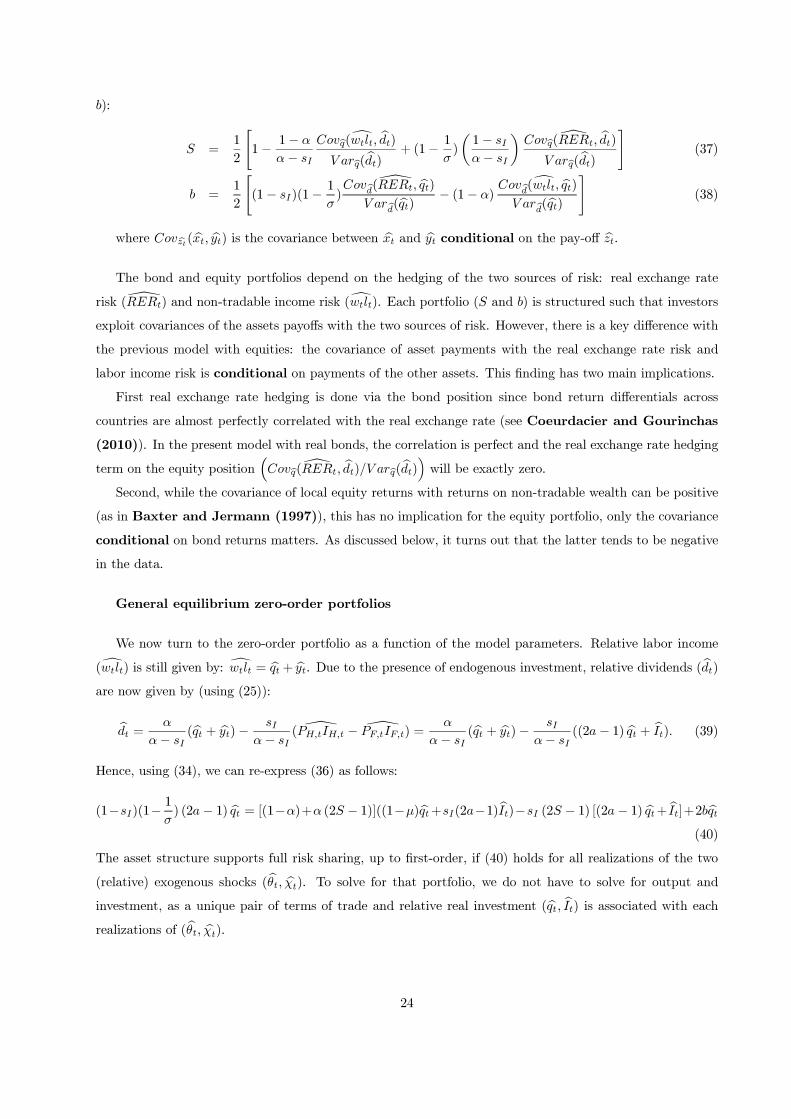
b):

S =1

2

[1−

1− α

α− sI

Covq(wtlt, dt)

V arq(dt)+ (1−

1

σ)

(1− sIα− sI

)Covq(RERt, dt)

V arq(dt)

](37)

b =1

2

[(1− sI)(1−

1

σ)Covd(RERt, qt)

V ard(qt)− (1− α)

Covd(wtlt, qt)

V ard(qt)

](38)

where Covzt(xt, yt) is the covariance between xt and yt conditional on the pay-off zt.

The bond and equity portfolios depend on the hedging of the two sources of risk: real exchange rate

risk (RERt) and non-tradable income risk (wtlt). Each portfolio (S and b) is structured such that investors

exploit covariances of the assets payoffs with the two sources of risk. However, there is a key difference with

the previous model with equities: the covariance of asset payments with the real exchange rate risk and

labor income risk is conditional on payments of the other assets. This finding has two main implications.

First real exchange rate hedging is done via the bond position since bond return differentials across

countries are almost perfectly correlated with the real exchange rate (see Coeurdacier and Gourinchas

(2010)). In the present model with real bonds, the correlation is perfect and the real exchange rate hedging

term on the equity position(Covq(RERt, dt)/V arq(dt)

)will be exactly zero.

Second, while the covariance of local equity returns with returns on non-tradable wealth can be positive

(as in Baxter and Jermann (1997)), this has no implication for the equity portfolio, only the covariance

conditional on bond returns matters. As discussed below, it turns out that the latter tends to be negative

in the data.

General equilibrium zero-order portfolios

We now turn to the zero-order portfolio as a function of the model parameters. Relative labor income

(wtlt) is still given by: wtlt = qt+ yt. Due to the presence of endogenous investment, relative dividends (dt)

are now given by (using (25)):

dt =α

α− sI(qt + yt)−

sIα− sI

( PH,tIH,t − PF,tIF,t) =α

α− sI(qt + yt)−

sIα− sI

((2a− 1) qt + It). (39)

Hence, using (34), we can re-express (36) as follows:

(1−sI)(1−1

σ) (2a− 1) qt = [(1−α)+α (2S − 1)]((1−µ)qt+sI(2a−1)It)−sI (2S − 1) [(2a− 1) qt+ It]+2bqt

(40)

The asset structure supports full risk sharing, up to first-order, if (40) holds for all realizations of the two

(relative) exogenous shocks (θt, χt). To solve for that portfolio, we do not have to solve for output and

investment, as a unique pair of terms of trade and relative real investment (qt, It) is associated with each

realizations of (θt, χt).

24

The following portfolio (S, b) ensures that (40) holds for arbitrary realizations of (qt, It):

S =1

2

[1 +

(2a− 1)(1− α)

1− (2a− 1)α

]>1

2, (41)

b =1

2

[(1− sI)(1−

1

σ) (2a− 1) +

(1− α)[µ− 1 + sI(2aI − 1)

2]

1− (2a− 1)α

](42)

The equity portfolio features home bias and is the sum of two terms only. The hedging-term for the real

exchange rate is indeed zero in this model since relative price movements are fully hedged by the appropriate

(real) bond position (cross-country differentials in bond payments are perfectly correlated with the real

exchange rate).

(i) The first term 12 is still the Lucas (1982) term which prevails in the absence of non-tradable income

risk (α→ 1)

(ii) The second term (2a−1)(1−α)1−(2a−1)α is the hedging of non-tradable income risk conditionally on bond pay-

ments: this term is unambiguously positive and drives home equity bias in the model. To understand

this term, assume a combination of shocks (θt, χt) such that relative investment It increases but leaves

the terms-of-trade (bond payments differential) qt unchanged. Such a combination of shocks will in-

crease labor demand and labor incomes since investment spending is using more intensively local goods

(a > 1/2).28 In the mean time, dividends net of investment spending are falling. This generates nega-

tive comovements between labor income and dividends holding relative prices constant (or equivalently

conditional on bond payments differentials).

The equity portfolio is the same as in Heathcote and Perri (2008)29 but holds for all values of the

preference parameters. In their benchmark case, parameters are such that σ = φ = µ = 1. In that case,

only fluctuations in investment matters for the equity portfolio, for two reasons: (i) fluctuations in output

are hedged through terms-of-trade movements (as in Cole and Obstfeld (1991)) due to µ = 1; (ii) σ = 1

cancels out any real exchange rate hedging term. As a consequence, the equity portfolio is the same as in

the present model. In contrast to the equities-only model, the equity portfolio in our model with bonds

and equity is remarkably stable to changes in preference parameters (see Coeurdacier and Gourinchas

(2010)).

The bond portfolio b is also the sum of two terms:

(i) The first term 12(1− sI)(1−

1σ ) (2a− 1) is the hedging of real exchange rate risk. This is the desired

exposure to real exchange rate in the absence of non-tradable income risk (α→ 1). This term is

unambiguously positive since local bonds have higher payoffs when local goods are more expensive.

28Note that with a = 1/2, this term is equal to zero since increases in domestic investment changes do not increase moredomestic demand than foreign. Wages increase as much in both countries.

29They consider the same model but with equities and productivity shocks only.

25

(ii) The second term(1−α)[µ−1+sI(2aI−1)2]

1−(2a−1)α is the hedging of non-tradable income risk conditionally on

relative dividend payments: this term can be positive or negative. Roughly speaking, it is negative if

relative wages are positively (resp. negatively) correlated with the terms-of-trade, which happens for

low values of µ, i.e. low elasticity of substitution φ (resp. for high values of µ, i.e. high elasticity of

substitution φ).

4.2.4 Empirical evidence on the hedging of non-tradable income risk

In order to show the relevance of conditioning for bond returns, we now present some empirical evidence on

the hedging of non-tradable risk (seeCoeurdacier, Kollmann and Martin (2010) for similar evidence30).

The evidence is based on the expression of the portfolio in terms of variance/covariance ratio (equation (37))

We use national accounts data for G7 countries to compute the conditional covariance-variance ratio(Covq(wtlt, dt)/V arq(dt)

)for each country. Data are quarterly over the period 1980Q1-2008Q3. Data are

taken from OECD National Accounts Data and from the IFS for exchange rates and price indices (see

Coeurdacier and Gourinchas (2010) for a precise description of the data). We compute relative labor

income deviations wtlt and relative dividend deviations dt for each country with respect to the other six

countries (wages are computed for each country as the share of output going to labor and dividends are

computed as the share of output going to capital net of investment spending).31 Deviations are either first-

difference of the variables or HP-filtered data (smoothing parameter 1600). We compute bond payments

differentials q using the (trade-weighted) real exchange rate of one country with respect to the other six. Note

that results are virtually the same when using nominal exchange rate instead of the real exchange rate (i.e.

considering nominal bonds instead of real bonds). We also report the unconditional covariance-variance

ratio(Cov(wtlt, dt)/V ar(dt)

), the one that matter in an equity-only model (see equation (18)). As shown in

table (2), conditioning for exchange rate movements has a strong impact on the hedging properties of equities

for non-tradable income risk: unconditionally (lines (1) and (3)), wages and dividends comove positively

for all countries, which would lead to a large foreign equity bias in the equity-only model of section (4.1).

Conditionally (lines (2) and (4), wages and dividends comove negatively for all countries, which lead to a

home equity bias in our equity-bond model. The presence of bonds makes the international diversification

puzzle better than you think, both in the model and in the data!

30In a revised version, Heathcote and Perri (2009) also provides similar empirical evidence.31We follow Gollin (2002) to allocate mixed-incomes from the national accounts to labor or capital. We assume that the

share of mixed income going to labor is equal to the share of labor income in value added.

26

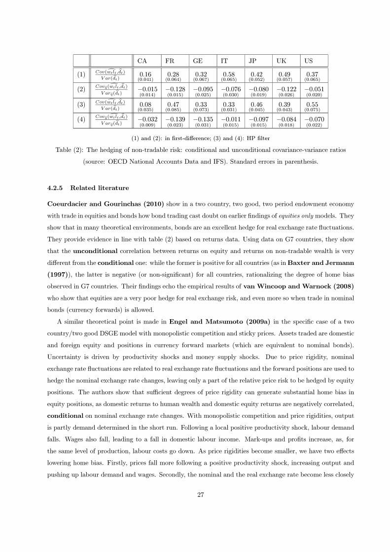
CA FR GE IT JP UK US

(1) Cov(wtlt,dt)

V ar(dt)0.16(0.041)

0.28(0.064)

0.32(0.067)

0.58(0.065)

0.42(0.052)

0.49(0.057)

0.37(0.065)

(2)Covq(wtlt,dt)

V arq(dt)−0.015(0.014)

−0.128(0.015)

−0.095(0.025)

−0.076(0.030)

−0.080(0.019)

−0.122(0.026)

−0.051(0.020)

(3) Cov(wtlt,dt)

V ar(dt)0.08(0.035)

0.47(0.085)

0.33(0.073)

0.33(0.031)

0.46(0.045)

0.39(0.043)

0.55(0.075)

(4)Covq(wtlt,dt)

V arq(dt)−0.032(0.009)

−0.139(0.023)

−0.135(0.031)

−0.011(0.015)

−0.097(0.015)

−0.084(0.018)

−0.070(0.022)

(1) and (2): in first-difference; (3) and (4): HP filter

Table (2): The hedging of non-tradable risk: conditional and unconditional covariance-variance ratios

(source: OECD National Accounts Data and IFS). Standard errors in parenthesis.

4.2.5 Related literature

Coeurdacier and Gourinchas (2010) show in a two country, two good, two period endowment economy

with trade in equities and bonds how bond trading cast doubt on earlier findings of equities only models. They

show that in many theoretical environments, bonds are an excellent hedge for real exchange rate fluctuations.

They provide evidence in line with table (2) based on returns data. Using data on G7 countries, they show

that the unconditional correlation between returns on equity and returns on non-tradable wealth is very

different from the conditional one: while the former is positive for all countries (as inBaxter and Jermann

(1997)), the latter is negative (or non-significant) for all countries, rationalizing the degree of home bias

observed in G7 countries. Their findings echo the empirical results of van Wincoop and Warnock (2008)

who show that equities are a very poor hedge for real exchange risk, and even more so when trade in nominal

bonds (currency forwards) is allowed.

A similar theoretical point is made in Engel and Matsumoto (2009a) in the specific case of a two

country/two good DSGE model with monopolistic competition and sticky prices. Assets traded are domestic

and foreign equity and positions in currency forward markets (which are equivalent to nominal bonds).

Uncertainty is driven by productivity shocks and money supply shocks. Due to price rigidity, nominal

exchange rate fluctuations are related to real exchange rate fluctuations and the forward positions are used to

hedge the nominal exchange rate changes, leaving only a part of the relative price risk to be hedged by equity

positions. The authors show that sufficient degrees of price rigidity can generate substantial home bias in

equity positions, as domestic returns to human wealth and domestic equity returns are negatively correlated,

conditional on nominal exchange rate changes. With monopolistic competition and price rigidities, output

is partly demand determined in the short run. Following a local positive productivity shock, labour demand

falls. Wages also fall, leading to a fall in domestic labour income. Mark-ups and profits increase, as, for

the same level of production, labour costs go down. As price rigidities become smaller, we have two effects

lowering home bias. Firstly, prices fall more following a positive productivity shock, increasing output and

pushing up labour demand and wages. Secondly, the nominal and the real exchange rate become less closely

27

related, making forward contracts less able to hedge fluctuations in relative prices. In the extreme case of

full price flexibility, we go back to Baxter and Jermann (1997): labor incomes and profits are perfectly

correlated and investors do not take any forward position as they do not want any exposure to purely

nominal risk. Engel and Matsumoto (2009b) generalise the results above to the cases of local bias in

consumption, producer currency pricing and wage rigidity.

Rabhari (2009) develops a two-country DSGE model with price stickiness, endogenous capital accu-

mulation, trade in nominal bonds and equities and endogenous monetary policy. In his setting, equity home

bias is again driven by the motive to hedge human capital risk. Real exchange rate risk is mainly hedged

through bond positions due to price stickiness. He also shows that the combination of price stickiness and

endogenous capital accumulation can produce relative equity returns that are unconditionally positively cor-

related with human capital returns, but conditionally negatively correlated (controlling for bond returns).

This correlation pattern is confirmed using US data.

Devereux and Sutherland (2007, 2008b) develops a two country, two good DSGE model with

nominal rigidities a la Calvo, producer currency pricing and endogenous monetary policy. The monetary

authority sets the nominal interest rate in response to changes in producer price inflation. There is no local

bias in consumption and productivity shocks are assumed to be persistent. The authors consider different

asset market structures (portfolio autarky, trade in nominal bonds and trade in nominal bonds and equity).

They can generate home bias in equities for the same reason as Engel and Matsumoto (2008a). They

also find that monetary policy assumes an additional role in these models. By changing the returns on

nominal bonds, monetary policy affects portfolios and thus risk sharing. Interestingly, they find that while

monetary policy has no impact on portfolios with trading in nominal bonds and equities, in the case of bond

trading only, there is an additional motive for price stability. With price stability, cross-country nominal

bonds returns differentials become more correlated with the real exchange rate, which improves international

risk sharing.

Lastly, Berriel and Bhattarai (2008) solves for equity and nominal bonds portfolios in a standard two-

country general equilibrium model in presence of government spending shocks and nominal shocks (shocks

to the price level): they investigate a new source of non-tradable income risk, namely tax changes. In order

to hedge fluctuations in taxes, households exhibit home bias towards local (government) nominal bonds and

local equities. The main mechanism goes as follows: price level shocks at home (increase in home inflation)

lowers the value of home government debt and the government can lower taxes (while still satisfying its

intertemporal constraint). Hence, returns on domestic nominal bonds and local taxes comove positively and

the household prefers to hold local nominal bonds. Government spending shocks lead to an increase in taxes.

In the mean time, as government expenditures are biased towards local goods, the relative price of locally

produced goods increase and so does the pay-off of the claim to local output (local equity). Hence, returns

on local equity and taxes comove positively and households will optimally bias their portfolio towards local

equity.

28

4.3 Extensions and shortcomings

4.3.1 Other assets?

The recent literature has shown the importance of extending existing models to a larger menu of assets. Due

to substitution across asset classes, the hedging role of an asset is modified by the presence of other available

types of assets. Thus, an important issue is why we should restrict our attention to bonds and equities

instead of considering an even larger set of assets. There is no simple answer to this question: potentially

any asset that is traded publicly could affect the equity portfolio if it has some hedging properties in addition

to what bonds and equities can achieve. Note that the empirical tests of these hedging properties based

on covariance-variance ratios could be potentially extended to a larger menu of assets, one just needs to

condition for returns on these other assets. In particular, including housing as an additional asset seems a

natural extension of existing work.

A related question is the role of corporate debt in these models. We have ignored debt as a way to raise

capital for firms and have focused on firms that are fully financed through equity. Coeurdacier, Kollmann

and Martin (2010) tackle this issue by allowing for an exogenous financial structure of firms in a world

of ‘locally complete’ markets. They show that in an environment where the financial structure is irrelevant

for the value of the firm (when the Modigliani-Miller theorem applies), the presence of corporate debt has

no impact on investment decisions and the equilibrium consumption allocation (up to the first order) since

markets are complete. Moreover, the equilibrium equity portfolio is also not affected by the presence of

corporate debt. They show that domestic investors will hold a fraction of the corporate debt issued by

domestic firms that is equal to the fraction of stocks of the same firms that they hold. Hence, if the model

delivers home bias in equity, it will also deliver home bias in corporate debt in the same proportion. The

reason is simple: when the Modigliani-Miller theorem applies, investors want a certain exposure to the total

value of the firm, which is independent of its financial structure. In particular, the fraction of the value

of the firm they hold optimally is pinned down in the case where firms are fully financed through equity.

When firms are partially financed through debt, holding the same fraction of debt and equity guarantees that

investors have their optimal exposure to the value of the firm. One shortcoming though is that such a result

might not hold if the Modigliani-Miller theorem does not apply or if financial markets are incomplete. We

are not aware of any models that pins down international portfolios in a world where the financial structure

of firm, optimal or not, affects the value of the firm and matters for the real allocation.

4.3.2 Exchange Rates and Asset Prices

While the models described above can claim some success in replicating some features of aggregate portfolio

data, they cannot replicate realistic moments of asset prices and exchange rates (see Lewis (2011) for

a recent survey on international asset pricing puzzles). They do not solve the standard puzzles in the

finance literature regarding the equity premium and the volatility of asset prices and exchange rates. This

is an important limitation since portfolios should be the mirror of asset prices as both are determined

29

in equilibrium. This does not mean that the mechanisms highlighted would not survive in more general

environments able to generate realistic asset prices but this remains to be seen. First attempts in that

direction include Stathopoulos (2008,2009) who introduces habit formation and Benigno and Nistico

(2009) who model ambiguity aversion. Interestingly, Benigno and Nistico (2009) show that, taking into

account long run consumption risk, which is correlated with the real exchange rate, changes the properties

of the pricing kernel and rationalizes home bias. We believe that explaining asset prices moments should

help disentangling across the different potential channels generating portfolio biases.

An important related shortcoming of this class of models with endogenous portfolio decisions is that the

allocation under perfect risk-sharing is replicated, or at least up to the degree of the approximation. This

implies an equality between the ratio of marginal utilities of consumption and the real exchange rate in all

states of nature. With standard CRRA preferences, this leads to a perfect correlation between real exchange

rate changes and relative consumption growth (Home relative consumption falls when Home relative prices

are higher; see equation (14) in the previous models). In the data, this is strongly rejected, the correlation is

close to zero and if anything Home relative consumption increases when Home relative prices are higher: this

is the famous consumption-real exchange rate anomaly (Kollmann-Backus-Smith puzzle; see Backus and

Smith (1993) and Kollmann (1995)). In the previous models, the asset structure and the dimension of

uncertainty are such that one can replicate the efficient allocation (up to first order). One could believe that

adding additional sources of uncertainty such that markets are incomplete even locally would help to solve

the consumption-real exchange rate anomaly. It turns out to be extremely hard to lower the correlation

between relative consumption and the real exchange rate in models with endogenous portfolio decisions

despite imperfect spanning of risks (see Coeurdacier, Kollmann and Martin (2007) and Benigno

and Kucuk-Tuger (2009)). In most existing models with endogenous portfolio choice, international risk-

sharing is still far above what consumption data suggests and this remains an important challenge for future

work.

4.3.3 Dispersion of home bias across time, countries and assets

Data on home bias exhibit substantial variations across time and across countries (see Figures (1) and (2)

and Table (1)). Most of the work has been dedicated to match the average degree of home bias observed in

developed countries (Collard et al. (2007) and Heathcote and Perri (2008) are notable exceptions:

in line with model predictions, they match the degree of equity bias to the degree of trade openness of

countries). Since more data on aggregate foreign asset holdings are now available, both in the time series

and in the cross-section, it seems natural to extend theories to heterogeneous countries. This would provide

more accurate tests of the different theories available. Exploiting the bilateral dimension of the data using a

multi-country framework could also help in that matter. Indeed, using the CPIS data provided by the IMF

since 2001, one can now observe equity holdings between country pairs. Most of the theoretical literature

has so far limited its attention to models with two symmetric countries, which does not allow to exploit the

30

bilateral and cross-sectional variations of the data.

A similar point can be made regarding the currency exposure of international portfolios. As shown by

Lane and Shambaugh (2009ab), the currency denomination of foreign assets and liabilities are very

heterogeneous across countries. While, on average, the advanced countries are (in net terms) borrowing

in foreign-currency, some major countries have very large negative domestic-currency debt positions (most

notably the US). Models including bond positions denominated in different currencies should be also tested

against such data. In section (7), we also provide some evidence on the cross sectional dispersion of home

bias for other asset classes (bonds and banking assets).

5 Asset trade costs in international financial markets

So far, we have focused on hedging motives as a source of heterogeneity in portfolios assuming frictionless

financial markets. Another strand of the macroeconomics literature considers frictions in financial markets

as the main source of heterogeneity across investors. Portfolio home bias is the natural outcome of these

frictions. Such frictions could include fixed or proportional transaction costs in foreign portfolio invest-

ments, difference of tax treatments across domestic and foreign portfolio incomes and other policy induced

restrictions on foreign investments (such as limits to foreign investment, capital controls, differences in legal

frameworks) (see French and Poterba (1991), Lewis (1999), Stulz et al. (2003)). Other important

frictions to international investments are informational frictions. The role of information has been exten-

sively investigated in the finance literature but less so in the Open Financial Macroeconomics literature

(Hatchondo (2008), Tille and van Wincoop (2009) and Dumas et al. (2011) are recent notable

exceptions). For this reason, we will review the literature on informational frictions (and behavioural biases)

in a separate section (see section (6)).

5.1 Transaction costs would need to be very large to explain equity home bias...

There is a wide debate on the importance of transaction costs to explain international portfolio decisions.

French and Poterba (1991) initially argue in a mean-variance framework that these costs must be much

larger than the one typically observed if one want to rationalize equity home bias. Using stock returns

data from 1975 to 1989 for the US, Japan, UK, France, Germany, Canada, the authors use estimates of a

covariance matrix of returns together with an optimal portfolio rule that is implied by constant relative risk

aversion in order to back out the differences in expected returns needed to explain actual portfolio shares

for these countries. The implicit excess return on domestic equity implied by observed portfolio holdings

is then interpreted as a measure of the cost of international asset trading needed to generate the observed

home bias: they find an order of magnitude for these costs of several hundred basis points, too big to

be true! Numerous subsequent studies have provided such indirect estimates of the costs. Jeske (2001)

calculates the implicit costs on foreign assets necessary to skew the portfolio allocation away from the optimal

(based on a mean variance model) toward the observed allocation. These costs are very large ranging from

31

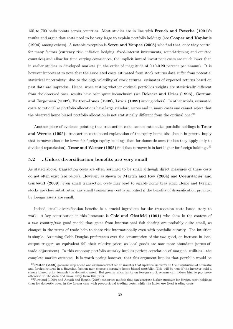
150 to 700 basis points across countries. Most studies are in line with French and Poterba (1991)’s

results and argue that costs need to be very large to explain portfolio holdings (see Cooper and Kaplanis

(1994) among others). A notable exception is Sercu and Vanpee (2008) who find that, once they control

for many factors (currency risk, inflation hedging, fixed-interest investments, round-tripping and omitted

countries) and allow for time varying covariances, the implicit inward investment costs are much lower than

in earlier studies in developed markets (in the order of magnitude of 0.10-0.20 percent per annum). It is

however important to note that the associated costs estimated from stock returns data suffer from potential

statistical uncertainty: due to the high volatility of stock returns, estimates of expected returns based on

past data are imprecise. Hence, when testing whether optimal portfolios weights are statistically different

from the observed ones, results have been quite inconclusive (see Bekaert and Urias (1996), Gorman

and Jorgensen (2002), Britten-Jones (1999), Lewis (1999) among others). In other words, estimated

costs to rationalize portfolio allocations have large standard errors and in many cases one cannot reject that

the observed home biased portfolio allocation is not statistically different from the optimal one.32

Another piece of evidence pointing that transaction costs cannot rationalize portfolio holdings is Tesar

and Werner (1995): transaction costs based explanation of the equity home bias should in general imply

that turnover should be lower for foreign equity holdings than for domestic ones (unless they apply only to

dividend repatriation). Tesar andWerner (1995) find that turnover is in fact higher for foreign holdings.33

5.2 ...Unless diversification benefits are very small

As stated above, transaction costs are often assumed to be small although direct measures of these costs

do not often exist (see below). However, as shown by Martin and Rey (2004) and Coeurdacier and

Guibaud (2009), even small transaction costs may lead to sizable home bias when Home and Foreign

stocks are close substitutes: any small transaction cost is amplified if the benefits of diversification provided

by foreign assets are small.

Indeed, small diversification benefits is a crucial ingredient for the transaction costs based story to

work. A key contribution in this literature is Cole and Obstfeld (1991) who show in the context of

a two country/two good model that gains from international risk sharing are probably quite small, as

changes in the terms of trade help to share risk internationally even with portfolio autarky. The intuition

is simple. Assuming Cobb Douglas preferences over the consumption of the two good, an increase in local

output triggers an equivalent fall their relative prices as local goods are now more abundant (terms-of-

trade adjustment). In this economy portfolio autarky implies perfect correlation of marginal utilities - the

complete market outcome. It is worth noting however, that this argument implies that portfolio would be

32Pastor (2000) goes one step ahead and examines whether an investor that updates his views on the distribution of domesticand foreign returns in a Bayesian fashion may choose a strongly home biased portfolio. This will be true if the investor hold astrong biased prior towards the domestic asset. But greater uncertainty on foreign stock returns can induce him to pay moreattention to the data and move away from this prior.

33Rowland (1999) and Amadi and Bergin (2008) construct models that can generate higher turnover for foreign asset holdingsthan for domestic ones, in the former case with proportional trading costs, while the latter use fixed trading costs.

32

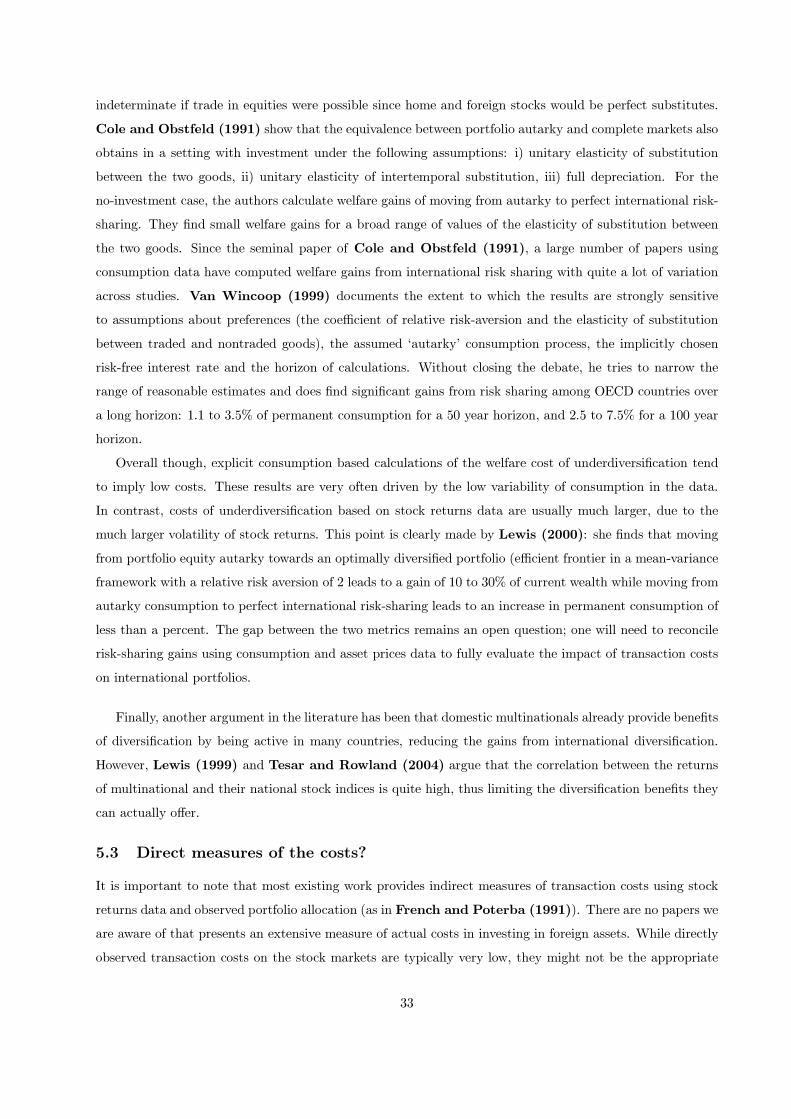
indeterminate if trade in equities were possible since home and foreign stocks would be perfect substitutes.

Cole and Obstfeld (1991) show that the equivalence between portfolio autarky and complete markets also

obtains in a setting with investment under the following assumptions: i) unitary elasticity of substitution

between the two goods, ii) unitary elasticity of intertemporal substitution, iii) full depreciation. For the

no-investment case, the authors calculate welfare gains of moving from autarky to perfect international risk-

sharing. They find small welfare gains for a broad range of values of the elasticity of substitution between

the two goods. Since the seminal paper of Cole and Obstfeld (1991), a large number of papers using

consumption data have computed welfare gains from international risk sharing with quite a lot of variation

across studies. Van Wincoop (1999) documents the extent to which the results are strongly sensitive

to assumptions about preferences (the coefficient of relative risk-aversion and the elasticity of substitution

between traded and nontraded goods), the assumed ‘autarky’ consumption process, the implicitly chosen

risk-free interest rate and the horizon of calculations. Without closing the debate, he tries to narrow the

range of reasonable estimates and does find significant gains from risk sharing among OECD countries over

a long horizon: 1.1 to 3.5% of permanent consumption for a 50 year horizon, and 2.5 to 7.5% for a 100 year

horizon.

Overall though, explicit consumption based calculations of the welfare cost of underdiversification tend

to imply low costs. These results are very often driven by the low variability of consumption in the data.

In contrast, costs of underdiversification based on stock returns data are usually much larger, due to the

much larger volatility of stock returns. This point is clearly made by Lewis (2000): she finds that moving

from portfolio equity autarky towards an optimally diversified portfolio (efficient frontier in a mean-variance

framework with a relative risk aversion of 2 leads to a gain of 10 to 30% of current wealth while moving from

autarky consumption to perfect international risk-sharing leads to an increase in permanent consumption of

less than a percent. The gap between the two metrics remains an open question; one will need to reconcile

risk-sharing gains using consumption and asset prices data to fully evaluate the impact of transaction costs

on international portfolios.

Finally, another argument in the literature has been that domestic multinationals already provide benefits

of diversification by being active in many countries, reducing the gains from international diversification.

However, Lewis (1999) and Tesar and Rowland (2004) argue that the correlation between the returns

of multinational and their national stock indices is quite high, thus limiting the diversification benefits they

can actually offer.

5.3 Direct measures of the costs?

It is important to note that most existing work provides indirect measures of transaction costs using stock

returns data and observed portfolio allocation (as in French and Poterba (1991)). There are no papers we

are aware of that presents an extensive measure of actual costs in investing in foreign assets. While directly

observed transaction costs on the stock markets are typically very low, they might not be the appropriate

33

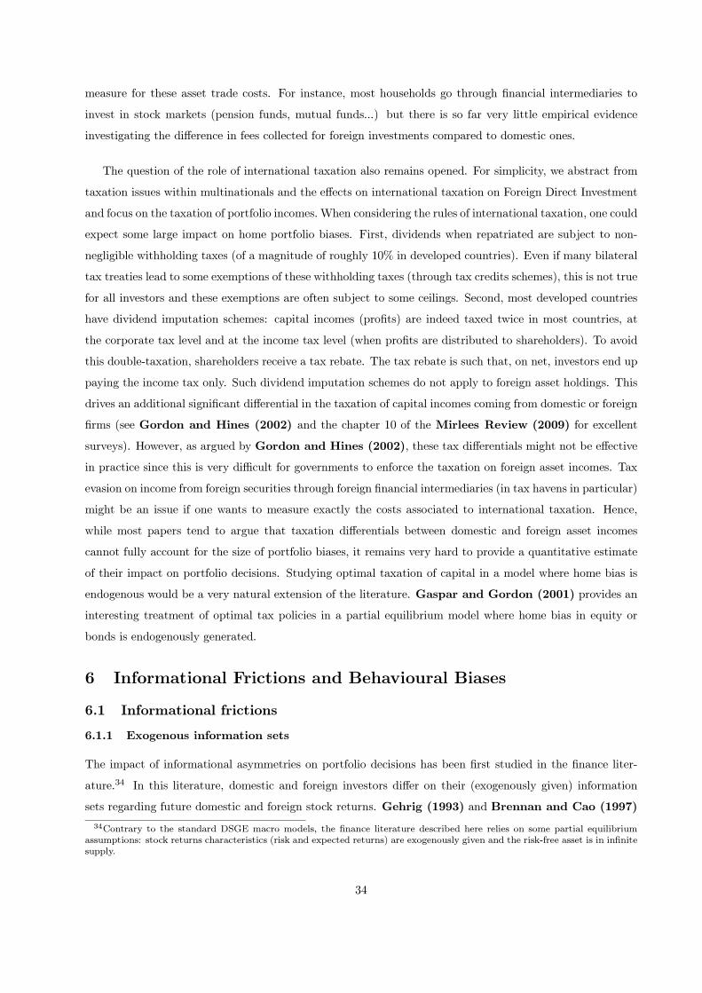
measure for these asset trade costs. For instance, most households go through financial intermediaries to

invest in stock markets (pension funds, mutual funds...) but there is so far very little empirical evidence

investigating the difference in fees collected for foreign investments compared to domestic ones.

The question of the role of international taxation also remains opened. For simplicity, we abstract from

taxation issues within multinationals and the effects on international taxation on Foreign Direct Investment

and focus on the taxation of portfolio incomes. When considering the rules of international taxation, one could

expect some large impact on home portfolio biases. First, dividends when repatriated are subject to non-

negligible withholding taxes (of a magnitude of roughly 10% in developed countries). Even if many bilateral

tax treaties lead to some exemptions of these withholding taxes (through tax credits schemes), this is not true

for all investors and these exemptions are often subject to some ceilings. Second, most developed countries

have dividend imputation schemes: capital incomes (profits) are indeed taxed twice in most countries, at

the corporate tax level and at the income tax level (when profits are distributed to shareholders). To avoid

this double-taxation, shareholders receive a tax rebate. The tax rebate is such that, on net, investors end up

paying the income tax only. Such dividend imputation schemes do not apply to foreign asset holdings. This

drives an additional significant differential in the taxation of capital incomes coming from domestic or foreign

firms (see Gordon and Hines (2002) and the chapter 10 of the Mirlees Review (2009) for excellent

surveys). However, as argued by Gordon and Hines (2002), these tax differentials might not be effective

in practice since this is very difficult for governments to enforce the taxation on foreign asset incomes. Tax

evasion on income from foreign securities through foreign financial intermediaries (in tax havens in particular)

might be an issue if one wants to measure exactly the costs associated to international taxation. Hence,

while most papers tend to argue that taxation differentials between domestic and foreign asset incomes

cannot fully account for the size of portfolio biases, it remains very hard to provide a quantitative estimate

of their impact on portfolio decisions. Studying optimal taxation of capital in a model where home bias is

endogenous would be a very natural extension of the literature. Gaspar and Gordon (2001) provides an

interesting treatment of optimal tax policies in a partial equilibrium model where home bias in equity or

bonds is endogenously generated.

6 Informational Frictions and Behavioural Biases

6.1 Informational frictions

6.1.1 Exogenous information sets

The impact of informational asymmetries on portfolio decisions has been first studied in the finance liter-

ature.34 In this literature, domestic and foreign investors differ on their (exogenously given) information

sets regarding future domestic and foreign stock returns. Gehrig (1993) and Brennan and Cao (1997)

34Contrary to the standard DSGE macro models, the finance literature described here relies on some partial equilibriumassumptions: stock returns characteristics (risk and expected returns) are exogenously given and the risk-free asset is in infinitesupply.

34

develop a simple two country noisy rational expectations model with one stock per country. They assume

that agents in each country receive a signal on the future performance of each stock but the signal on the

foreign asset is less precise. Hence, domestic investors perceive the foreign stock as riskier and reduce their

foreign stock holdings, which leads to equity home bias. Moreover, Brennan and Cao (1997) show that

less well informed foreign investors respond more strongly to public signals on domestic stocks conveyed by

stock prices. Hence foreign investors buy more of the domestic stocks when the domestic market performs

well. The authors find evidence for this ’return chasing’ effect in the data. Brennan and Cao (2005)

extend their initial work by developing a noisy expectations model where investors receive public and private

information signals. The private signal is less precise for foreign investors. The authors show that there is a

link between information disadvantages and the expectations (degree of bullishness) about a market: foreign

investors tend to become more bullish about a certain market following a positive return on that market.

Glassman and Riddick (2001) quantify what should be the perceived riskiness of foreign assets (due

to lower information quality) in order to generate the observed home bias of US investors. They find that

investors would have to scale up standard deviations of returns by a factor from 2 to 5 depending on risk

aversion and conclude that these scaling factors are implausibly high. Albuquerque et al. (2006) solve for

international equity flows when a set of home and foreign investors have superior information. They argue

that this informational heterogeneity within the foreign set of investors is more important than informational

heterogeneity across countries to explain international equity trades. In line with the data, the model ex-

plains why (i) U.S. investors trade in waves, with simultaneous buying and selling; (ii) U.S. investors change

their foreign equity positions gradually; and (iii) U.S. investors increase their equity position in a country

following a raise in its stock price.

The finance literature described above had a recent impact on more standard general equilibrium macro

models along the lines of the Open Economy Financial Macroeconomics approach. Hatchondo (2008)

builds a single good two country model and two assets per country with two departures from standard

models. Firstly, he assumes that only local investors receive informative signals about local assets. This

informational advantage induces agents to invest in the “good” local asset. Secondly, engaging in short

selling is assumed to be costly. When the signal is sufficiently informative and short selling costs are high

enough, agents do not sell the “bad” local asset short in order to invest more in the “good” local asset but

rather reduce their holdings of foreign assets. This leads to equity home bias in equilibrium. Bovenverg

and Gordon (1996), present a small open economy model where home bias results from information

asymmetries, which decrease the return home investors get on their foreign capital investment. In such a set

up, subsidizing capital imports is optimal. Razin et al. (1999) assume that domestic investors can observe

the productivity of domestic firms before making their loan decisions, while foreign investors cannot. This

results in foreign underinvestment and domestic oversaving. Building on a similar asymmetric information

set up but adding the possibility of liquidity shocks, Goldstein and Razin (2006) study the trade-off

between FDI and portfolio investment, the latter being more liquid than the former.

35

Tille and van Wincoop (2009) applies the noisy rational expectations framework from the finance

literature to a standard two country/one good DSGE model. They depart from standard open macro models

by introducing information dispersion across investors. Each investor receives a private signal on the future

fundamentals (productivity) of domestic and foreign stock, the signal on its own stock being more precise (as

in Gehrig (1993) and Brennan and Cao (1997)). The noise is introduced in the form of (unobserved)

stochastic transaction costs to invest abroad which generates portfolio shifts towards or away from foreign

assets. This makes sure that stock prices cannot fully aggregate private signals in equilibrium. These

transaction costs generate equity home bias in equilibrium but this is not the purpose of the paper. They

show that dispersed private information disconnects stock prices from the currently observed fundamental

values but also international capital flows (gross and net). Moreover, capital flows should help forecast future

fundamentals. They find some empirical support for their results.

6.1.2 Endogenous information acquisition

The early noisy rational expectations literature when applied to international portfolio choice relies on

exogenous information structures. A recent challenge has been to extend it by allowing for endogenous

information acquisition. In this line of research, information is a tool to reduce the conditional variance of

the asset payoffs. Using a model of rational inattention introduced by Sims (2001), Van Nieuwerburg

and Veldkamp (2009) build a model where a tiny information advantage is enough to generate significant

home bias if investors have a limited capacity to process information. In this model, agents are endowed with

a small informational advantage on the local asset, which lowers its perceived riskiness. Thus, the investor will

tend to hold more of the local asset. However, this effect is amplified as the more of an asset the agent owns,

the more attractive it becomes to learn about the asset. Endogenous and costly acquisition of information

amplifies the initial small informational advantage and leads to specialization in local stocks. Learning turns

out to amplify information asymmetries instead of reducing them. In their set up, countries which are learnt

about a lot by investors should have lower returns compared to the prediction of a standard CAPM model,

as lower uncertainty goes hand in hand with a lower return. Van Nieuwerburg and Veldkamp (2010)

apply variations of their rational inattention model to explain investment strategies of investors, varying the

specification of the preferences or of the information constraint that they face. Depending on the convexity

of the objective function of investors, they can rationalize concentrated or diversified portfolios. Mondria

(2010) allows rationally inattentive investors to decide not only on the precision but also on the structure of

the information they process. In equilibrium, agents choose to learn not only about individual assets but also

about linear combination of assets, i.e. indices. Such a learning strategy makes sense as the structure of the

signal the agents choose in equilibrium depends on their objective function. Since investors will choose to hold

a somewhat diversified portfolio in equilibrium, they choose to process information about combinations of

assets (they are interested not only in the volatility of each asset but also in their covariance). Mondria and

Wu (2010) use a similar framework to explain the time series of home bias. When financial liberalization

takes place in the developed economies in the 1980s, investors start to be able to diversify their portfolios

36

and home bias decreases but only gradually as investors have an initial information advantage on domestic

assets. The authors show that persistence of asset pay-offs and increases in information processing capacity

tends to magnify home bias. By looking at the interaction of capital openness and learning strategies, they

are able to reproduce the time series of home bias35.

6.1.3 Empirical evidence on informational frictions

A number of papers regress portfolio holdings or measures of home bias directly on factors that proxy for

information asymmetries. Portes and Rey (2005) shows that physical distance affects international equity

flows and holdings very significantly: doubling the distance reduces cross-border equity flows by half. Coval

and Moskowitz (1999) find that U.S. mutual fund managers prefer to invest in nearby firms even within

a country. Ahearne et al. (2004) find that U.S. holdings of foreign equities are significantly biased

towards countries that have a higher share of their stock market listed on U.S. stock exchanges. Chan

et al. (2005) find that stock market development and familiarity variables have a significant impact on

home bias for a sample of mutual funds spanning 26 developed and developing markets. They aggregate the

investments of these funds at the country level. Grinblatt and Keloharju (2001) emphasizes the key role

of distance, language and cultural similarities in international asset allocation. Aviat and Coeurdacier

(2007) revisits the impact of distance on cross-border equity holdings (and bank loans). They find that the

impact of distance is drastically reduced once we control for bilateral goods trade: countries portfolios are

strongly biased towards trading partners (see also Lane and Milesi Ferretti (2008)). Using instrumental

variables, they show that the causality goes essentially one-way: reducing barriers to trade in goods enhances

cross-border asset holdings. However, one cannot reject the role of goods trade in fostering information flows

across borders. Since a lot of information on stocks come through the accounts of firms, it is to be expected

that different accounting standards would act as information barriers. Bradshaw, Bushee, and Miller

(2004) find that firms exhibiting higher levels (changes) of U.S. GAAP conformity have greater levels

(changes) of U.S. institutional ownership. This positive relation holds regardless of a firm’s visibility to

U.S. investors (e.g., American Depositary Receipt listing, stock index membership, analyst following, firm

size). Finally, using survey data on Italian investors, Guiso and Japelli (2006) find that investors who

spend more time to acquire information also tend to hold less diversified portfolios as implied by models of

endogenous information acquisition.

Most models of information asymmetries though also imply that domestic investors should earn a higher

return than foreign investors. However, the empirical evidence on this matter is mixed. Coval and

Moskowitz (1999), Hau (2001), Dvorak (2005) and Choe et al (2005) find that domestic investors

do in fact earn higher returns, while Grinblatt and Keloharju (2000) and Huang and Shiu (2006)

find the opposite.

35For a very nice exposition of the applications of rational inattention to invesment choice see Velkamp (2001).

37

6.2 Behavioural biases

Some recent papers have put forward a behavioral explanation for the equity home bias. Using departures

from rational expectations and maximization of standard von Neumann-Morgenstern utility functions used

in standard macro literature, this literature has highlighted some behavioural biases consistent with the data

on international portfolio allocation. The seminal paper of French and Poterba (1991) already consid-

ers overconfidence towards local assets as a potential explanation: if investors systematically have higher

expectations of relative returns for domestic equities, this difference in expected returns, while inconsistent,

can overturn any perceived diversification gains. In the same vein, Shiller et al. (1991) document large

differences in expected returns of Japanese and U.S. investors for the same stockmarkets. They find that

Japanese investors tend to expect relatively higher returns for Japanese stocks, while U.S. investors expect

higher returns on U.S. equity. A similar argument can be applied to estimated variances (either the standard

deviation of domestic equity is systematically believed to be lower or correlations with foreign equities are

overestimated). Studies by Huberman (2001), Benartzi (2001) and Karlsson and Norden (2007)

(see also Barberis and Thaler (2003) for a survey) suggest that ‘familiarity’ might be the main determi-

nant of portfolio choice: investors choose ‘familiar’ assets while ignoring the principles of portfolio theory.

Graham, Harvey and Huang (2009) investigates the role of self-assessed trading competences on port-

folio home bias. They show how home bias can emerge when investor feels incompetent in understanding the

benefits and the risks of investing in foreign assets. However, it remains difficult to disentangle empirically

informational frictions linked to distance and/or institutional differences from behavioural biases such as

‘familiarity’ and/or ‘competence’ effects. Solnik (2006) explains the equity home bias by the Regret The-

ory: investors use the domestic portfolio as a benchmark and feel the pain when their foreign investments

underperform. Finally,Morse and Shive (2006) find that home bias is empirically related to measures of

patriotism.

To our knowledge, building onDumas, Kurshev and Uppal (2007), Dumas, Lewis and Osambela

(2009) are the first ones to develop a standard two-country general equilibrium model (in continuous time)

where investors exhibit behavioural biases in the form of differences in their beliefs. Investors have access

to the same information set (no asymmetric information) but differ in their beliefs about the information

contained in economic public signals: local investors trust more the information contained in local signals

and incorrectly believe that the information in the foreign signal is partly noise. These asymmetric beliefs

help the authors to solve for some anomalies at the international level: investors exhibit home equity bias,

asset prices are the combination of a local CAPM and an international CAPM (in line with the empirical

evidence of Bekaert and Harvey (1995)) and as in models of asymmetric information (see Brennan and

Cao (2005)), capital flows towards a country covary positively with returns in that country. Their model

with differences in beliefs is indeed observationally equivalent to existing models of segmented markets due

to asymmetric information.

38

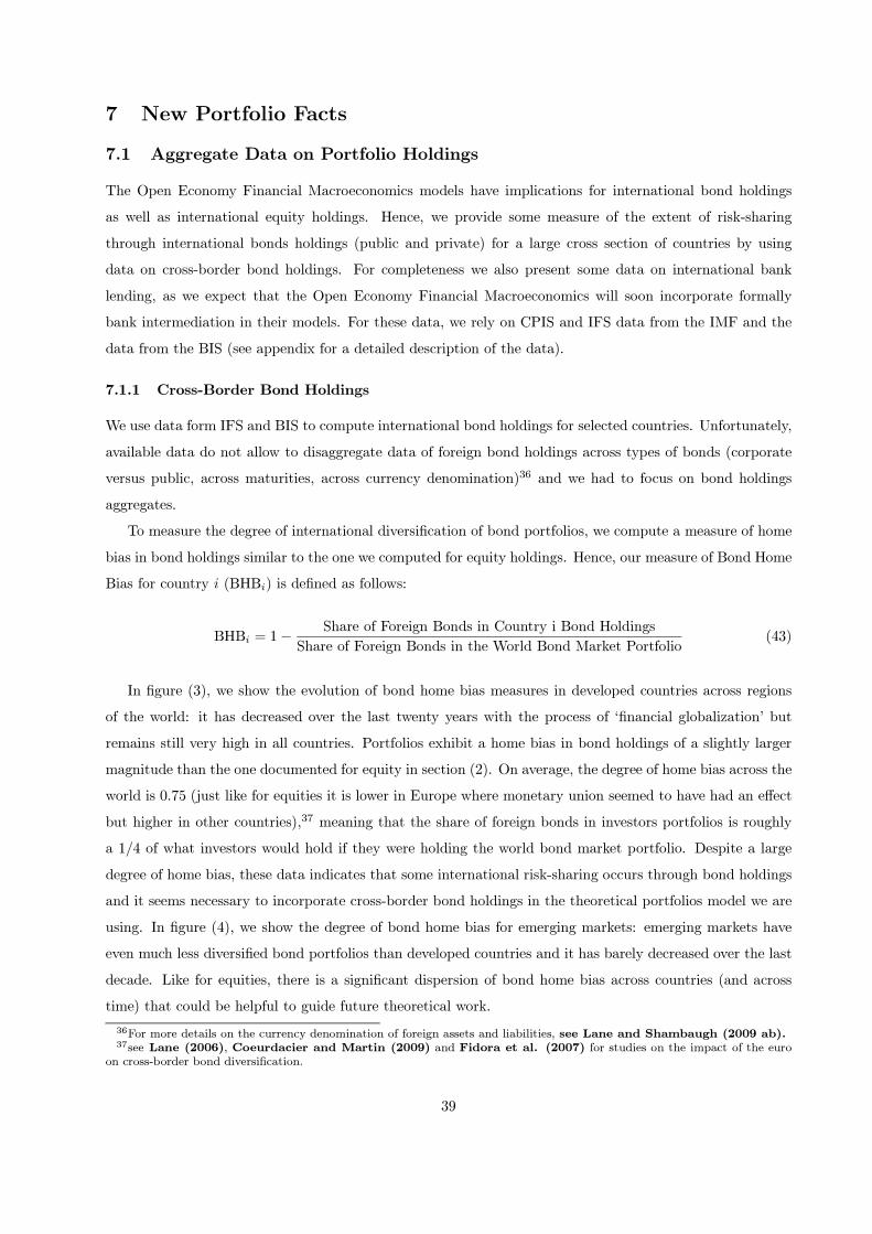
7 New Portfolio Facts

7.1 Aggregate Data on Portfolio Holdings

The Open Economy Financial Macroeconomics models have implications for international bond holdings

as well as international equity holdings. Hence, we provide some measure of the extent of risk-sharing

through international bonds holdings (public and private) for a large cross section of countries by using

data on cross-border bond holdings. For completeness we also present some data on international bank

lending, as we expect that the Open Economy Financial Macroeconomics will soon incorporate formally

bank intermediation in their models. For these data, we rely on CPIS and IFS data from the IMF and the

data from the BIS (see appendix for a detailed description of the data).

7.1.1 Cross-Border Bond Holdings

We use data form IFS and BIS to compute international bond holdings for selected countries. Unfortunately,

available data do not allow to disaggregate data of foreign bond holdings across types of bonds (corporate

versus public, across maturities, across currency denomination)36 and we had to focus on bond holdings

aggregates.

To measure the degree of international diversification of bond portfolios, we compute a measure of home

bias in bond holdings similar to the one we computed for equity holdings. Hence, our measure of Bond Home

Bias for country i (BHBi) is defined as follows:

BHBi = 1−Share of Foreign Bonds in Country i Bond Holdings

Share of Foreign Bonds in the World Bond Market Portfolio(43)

In figure (3), we show the evolution of bond home bias measures in developed countries across regions

of the world: it has decreased over the last twenty years with the process of ‘financial globalization’ but

remains still very high in all countries. Portfolios exhibit a home bias in bond holdings of a slightly larger

magnitude than the one documented for equity in section (2). On average, the degree of home bias across the

world is 0.75 (just like for equities it is lower in Europe where monetary union seemed to have had an effect

but higher in other countries),37 meaning that the share of foreign bonds in investors portfolios is roughly

a 1/4 of what investors would hold if they were holding the world bond market portfolio. Despite a large

degree of home bias, these data indicates that some international risk-sharing occurs through bond holdings

and it seems necessary to incorporate cross-border bond holdings in the theoretical portfolios model we are

using. In figure (4), we show the degree of bond home bias for emerging markets: emerging markets have

even much less diversified bond portfolios than developed countries and it has barely decreased over the last

decade. Like for equities, there is a significant dispersion of bond home bias across countries (and across

time) that could be helpful to guide future theoretical work.

36For more details on the currency denomination of foreign assets and liabilities, see Lane and Shambaugh (2009 ab).37see Lane (2006), Coeurdacier and Martin (2009) and Fidora et al. (2007) for studies on the impact of the euro

on cross-border bond diversification.

39

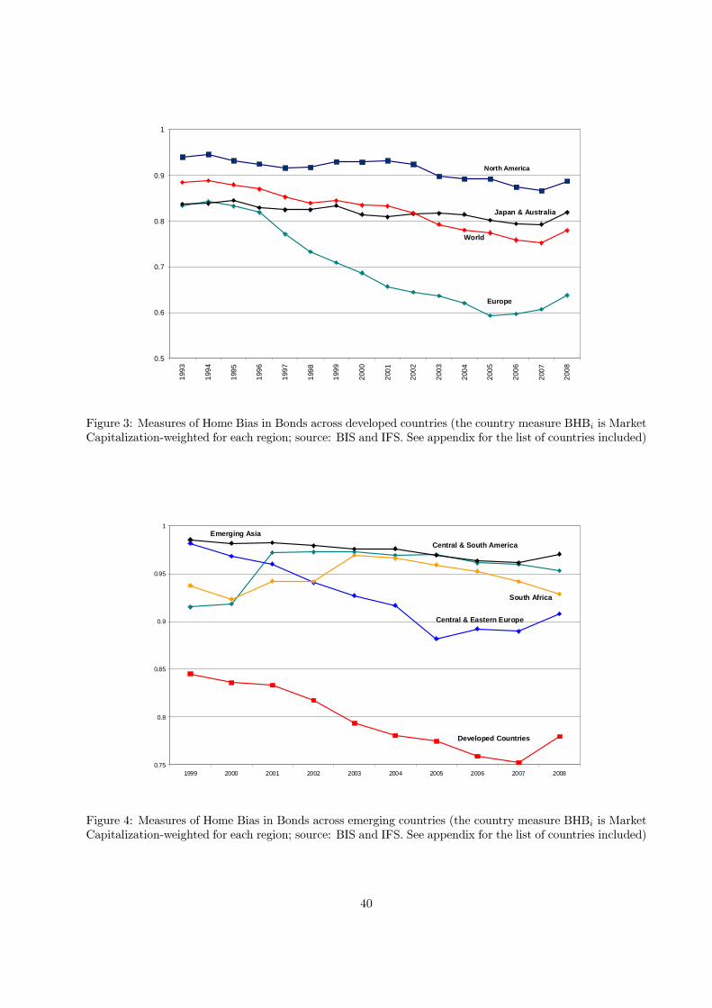
0.5

0.6

0.7

0.8

0.9

1

1993

1994

1995

1996

1997

1998

1999

2000

2001

2002

2003

2004

2005

2006

2007

2008

Europe

North America

Japan & Australia

World

Figure 3: Measures of Home Bias in Bonds across developed countries (the country measure BHBi is MarketCapitalization-weighted for each region; source: BIS and IFS. See appendix for the list of countries included)

0.75

0.8

0.85

0.9

0.95

1

1999 2000 2001 2002 2003 2004 2005 2006 2007 2008

Developed Countries

Central & Eastern Europe

South Africa

Emerging Asia

Central & South America

Figure 4: Measures of Home Bias in Bonds across emerging countries (the country measure BHBi is MarketCapitalization-weighted for each region; source: BIS and IFS. See appendix for the list of countries included)

40

7.1.2 Cross-Border Bank Loans

We use data from the BIS and the OECD to compute cross-border banking assets for selected countries.

Like for bonds, available data do not allow to disaggregate data of foreign bank loans across types of loans

and we had to focus on aggregate foreign asset holdings by banks.

To measure the degree of international diversification of banks’ portfolios, we compute a measure of home

bias in bank loans comparable to the one used for equities and bonds. Hence, our measure of Home Bias in

Loans for country i (LHBi) is defined as follows:

LHBi = 1−Share of Foreign Banking Assets in Country i Banking Assets

Foreign Banking Assets as a share of Total Foreign Outstanding Loans(44)

In figure (5), we show the evolution of home bias in bank loans measures across OECD countries using

OECD data. Figure (6) shows the same statistic but using BIS statistics (available for a larger number

of countries but over a shorter time period; see appendix for a detailed description of the data). Despite

an increased diversification, banking portfolios still exhibit a very strong home bias. The magnitude of the

home bias in banking assets is similar to the one observed for equity holdings. Like for equities and bonds,

the degree of Home Bias is the smallest in Europe (potentially due to the EMU) and the largest in emerging

markets (here Latin America).

7.2 Institutional Investors Home Bias Data

An increasing share of capital flows are intermediated through institutional investors. For example, using the

Survey of Consumer Finance, Polkovnichenko (2004) documents that in 2001, 62% of all equity holdings

by US households were indirect holdings. Information asymmetries explanations of the home bias seem

more plausible for households than for fund managers, who can devote a substantial amount of resources

to gather relevant information. Also, if home bias can be explained by the degree of sophistication of

investors regarding their investment strategies, one would expect that professional investors would be fully

aware of the theoretical benefits of diversification. Furthermore, with delegated investment comes an agency

problem and the incentives of the final investor and of the fund manager are not necessarily well aligned. It

should therefore be informative to look at portfolio allocations at the fund level to understand better the

determinants of home bias. Hau and Rey (2008) provides some descriptive statistics on domestic and

foreign holdings of mutual funds in 4 countries. We use the same data set - data of global equity holdings

from Thomson Financial Securities (TFS)- to estimate home bias at the fund level on a larger cross section of

countries. The data document individual mutual funds holdings at the stock level. TFS was created by the

merger of The Investext Group, Security Data Company and CDA/Spectrum. The data cover the five year

period 1997 to 2002 and has an interesting cross sectional and time series dimension.38 The TFS holding data

comprise fund number, fund name, management company name, country code of the fund incorporation,

38Chan et al. (2005) used a similar dataset -albeit only for one year. They aggregated the data across all funds to documenthome bias at the country level.

41

0.5

0.6

0.7

0.8

0.9

1

1995 1996 1997 1998 1999 2000 2001 2002 2003 2004 2005 2006 2007

Japan North America

World (OECD)

Europe

Figure 5: Measures of Home Bias in Banking assets across OECD countries (in each region, the countrymeasure LHBi is weighted by the share of oustanding loans of the country in the region; source: OECD. Seeappendix for the list of countries included)

0.6

0.7

0.8

0.9

1

2001 2002 2003 2004 2005 2006 2007 2008

Europe

World

North America

Japan

Central & South America

Figure 6: Measures of Home Bias in Banking assets across Regions (in each region, the country measureLHBi is weighted by the share of oustanding loans of the country in the region; source: BIS. See appendixfor the list of countries included)

42

stock identifier, country code of the stock, stock position (number of stocks held), reporting dates for which

holding data is available, security price on the reporting date and the security price on the closest previous

days in case the reporting date had no price information on the security, total return index (including

dividend reinvestments) in local currency, and daily dollar exchange rates for all investment destinations.

Most funds report only with a frequency of 6 months. Reporting dates differ somewhat, but more than 90

percent of the reporting occurs in the last 30 days of each half-year. A limitation of the data is that they

do not include any information on cash holdings, financial leverage, investments in fixed income instruments

or investments in derivative contracts. The portfolio characteristics we calculate therefore concern only the

equity proportion of a fund’s investment. Table 1 gives the breakdown of the average market capitalization

over the sample in billions of dollars by country of fund origin. Table 2 gives the breakdown of the average

number of funds also by country of fund origin.

Graph 1 present the percentage of mutual funds based in a given country whose shares of domestic

holdings in total asset holdings is 0%, strictly larger than 0% but smaller than 10%, between 10 and 20%,

.., between 90 and 100% (but strictly below 100%) and equal to 100%. The numbers are averages for the

1997-2002 period. To simplify, we call these different shares of domestic holdings in total holdings ”different

degrees of home bias”. For each country, the percentages are based on number of funds in a given home bias

category out of the total number of funds for that country and on the share of the market capitalization of

funds in a given category relative to the total market capitalization of funds of that country. Thus, funds

may change from one home bias category to another over the course of the sample.

The most striking stylized fact may be that there is a great deal of heterogeneity both across countries

and within country in the extent of domestic holdings in total holdings. For most countries, the distribution

usually exhibits peaks at 0% and 100% (or between 0 and 10% and between 90 and 100%) indicating sub-

stantial specialization of funds into either (close to) fully domestic or (close to) fully international investment.

But, interestingly, there is a non negligible part of the distribution lying in between those two extremes,

indicating a great deal of heterogeneity in diversification choices by the fund managers even within country.

Thus one conjecture is that the observed investment pattern at the fund level reflects both some increasing

returns in the information technology leading to some concentration in stock holdings of either domestic or

foreign countries and a particular market structure inducing product differentiation at the fund level. As

mentioned in Hau and Rey (2008), there is a positive correlation between the number of sectors and the

number of countries funds invest in, suggesting that more diversified funds diversify both across sectors of

activity and across countries. Larger funds tend also to be the most diversified. The role of fund mandates in

the observed asset holdings is of course of great interest. We find that for example, in 2002, 701 funds out of

our 1,291 US funds had some kind of explicit mandates, which could range from ”investing in world equities”

to ”primarily small cap north American companies” or ”at least 80% in Latin American companies”. These

mandates seem to exhibit considerable variations across countries and are clearly not exogenous. They too

result from the optimizing behaviour of financial companies. Explaining home bias or indeed investment

43

strategies at the fund level thus probably requires a theory of fund mandates.

8 Conclusions and leads for future research

Our view is that the home bias puzzle is now less of a puzzle. From the literature we labeled “Open Economy

Financial Macroeconomics” to the rational inattention models featuring endogenous information acquisition,

notable progress has been made to understand the determinants of portfolio allocations. We may now be

at a stage where we should be studying a broad array of implications of these new models rather than

focusing only on the stylized fact of equity home bias. Confronting their predictions with a large set of other

stylized facts on portfolio holdings will surely lead us to refine them further and ultimately assess their true

explanatory power.

The Open Economy Financial Macroeconomics literature has an interesting set of predictions on the

holdings of a broad menu of financial assets. It should be very fruitful to introduce in that literature some

more detailed models of the capital structure of firms and to get finer empirical implications for equities and

corporate/banking debt in particular. Applying corporate finance theory to model the capital structure of

firms seems a natural extension of these models, all the more so since it has been shown to matter empirically

to explain the home bias (see Dahlquist, Pinkowitz, Stulz, and Williamson (2003)). One major issue

going forward will also be the modelling of the official sector. Introducing an optimal monetary or fiscal

policy and modelling their interactions with endogenous portfolio choices of the private sector is a major

challenge. It is likely that as a first step focusing on realistic but not necessarily optimal monetary policy

or fiscal rules will be the way to go. It is an important goal to have realistic and workable macroeconomic

models of the open economy with endogenous portfolio choice, as large cross border holdings of assets (see

Gourinchas and Rey (2007a)) are likely to affect the channels of transmission of monetary and fiscal

policy. Understanding the short run dynamics of the exchange rate, a formidable but crucial task, is also

intimately linked to agents portfolio choices and gross external positions as shown in Gourinchas and

Rey (2007b) and Della Corte et al. (2009). Furthermore, a closer look at the maximization problems

faced by Central Banks when they decide on their reserve holdings and by sovereign wealth funds would be

warranted as both actors now account for a non trivial share of international capital flows. The portfolio

choice of the official sector is also an important determinant of the international use of a currency. The dollar

market share in world transactions and the ”exorbitant privilege” of the United States may be challenged by

the new portfolio diversification strategies of emerging markets in general and China in particular. We have

few models which can tackle these issues in a general equilibrium set up with a rich asset structure. The

role of international currencies and their importance in determining portfolios and asset price movements is

an area of active research (see Devereux and Shi (2009) or Gourinchas et al. (2010)).

As more detailed survey data on households become available, one will also be better able to test at the

microeconomic level the empirical relevance of various hedging motives underlying the mechanism of these

44

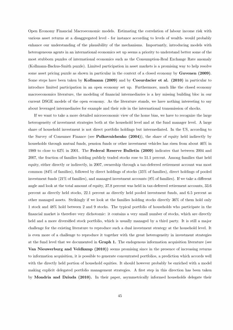
Open Economy Financial Macroeconomic models. Estimating the correlation of labour income risk with

various asset returns at a disaggregated level - for instance according to levels of wealth- would probably

enhance our understanding of the plausibility of the mechanisms. Importantly, introducing models with

heterogeneous agents in an international economics set up seems a priority to understand better some of the

most stubborn puzzles of international economics such as the Consumption-Real Exchange Rate anomaly

(Kollmann-Backus-Smith puzzle). Limited participation in asset markets is a promising way to help resolve

some asset pricing puzzle as shown in particular in the context of a closed economy by Guvenen (2009).

Some steps have been taken by Kollmann (2009) and by Coeurdacier et al. (2010) in particular to

introduce limited participation in an open economy set up. Furthermore, much like the closed economy

macroeconomics literature, the modeling of financial intermediaries is a key missing building bloc in our

current DSGE models of the open economy. As the literature stands, we have nothing interesting to say

about leveraged intermediaries for example and their role in the international transmission of shocks.

If we want to take a more detailed microeconomic view of the home bias, we have to recognize the large

heterogeneity of investment strategies both at the household level and at the fund manager level. A large

share of household investment is not direct portfolio holdings but intermediated. In the US, according to

the Survey of Consumer Finance (see Polkovnichenko (2004)), the share of equity held indirectly by

households through mutual funds, pension funds or other investment vehicles has risen from about 46% in

1989 to close to 62% in 2001. The Federal Reserve Bulletin (2009) indicates that between 2004 and

2007, the fraction of families holding publicly traded stocks rose to 51.1 percent. Among families that held

equity, either directly or indirectly, in 2007, ownership through a tax-deferred retirement account was most

common (84% of families), followed by direct holdings of stocks (35% of families), direct holdings of pooled

investment funds (21% of families), and managed investment accounts (8% of families). If we take a different

angle and look at the total amount of equity, 37.8 percent was held in tax-deferred retirement accounts, 33.6

percent as directly held stocks, 22.1 percent as directly held pooled investment funds, and 6.5 percent as

other managed assets. Strikingly if we look at the families holding stocks directly 36% of them hold only

1 stock and 48% hold between 2 and 9 stocks. The typical portfolio of households who participate in the

financial market is therefore very dichotomic: it contains a very small number of stocks, which are directly

held and a more diversified stock portfolio, which is usually managed by a third party. It is still a major

challenge for the existing literature to reproduce such a dual investment strategy at the household level. It

is even more of a challenge to reproduce it together with the great heterogeneity in investment strategies

at the fund level that we documented in Graph 1. The endogenous information acquisition literature (see

Van Nieuwerburg and Veldkamp (2010)) seems promising since in the presence of increasing returns

to information acquisition, it is possible to generate concentrated portfolios, a prediction which accords well

with the directly held portion of household equities. It should however probably be enriched with a model

making explicit delegated portfolio management strategies. A first step in this direction has been taken

by Mondria and Dziuda (2010). In their paper, asymmetrically informed households delegate their

45

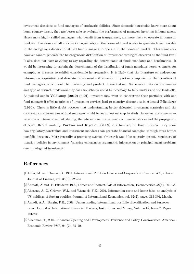
investment decisions to fund managers of stochastic abilities. Since domestic households know more about

home country assets, they are better able to evaluate the performance of managers investing in home assets.

Hence more highly skilled managers, who benefit from transparency, are more likely to operate in domestic

markets. Therefore a small information asymmetry at the household level is able to generate home bias due

to the endogenous decision of skilled fund managers to operate in the domestic market. This framework

however cannot generate the heterogeneous distribution of investment strategies observed at the fund level.

It also does not have anything to say regarding the determinants of funds mandates and benchmarks. It

would be interesting to explain the determinants of the distribution of funds mandates across countries for

example, as it seems to exhibit considerable heterogeneity. It is likely that the literature on endogenous

information acquisition and delegated investment still misses an important component of the incentives of

fund managers, which could be marketing and product differentiation. Some more data on the number

and type of distinct funds owned by each households would be necessary to fully understand the trade-offs.

As pointed out in Veldkamp (2010) (p101), investors may want to concentrate their portfolios with one

fund manager if efficient pricing of investmnet services lead to quantity discount as in Admati Pfleiderer

(1990). There is little doubt however that understanding better delegated investment strategies and the

constraints and incentives of fund managers would be an important step to study the extent and time series

variation of international risk sharing, the international transmission of financial shocks and the propagation

of crises. Recent work by Pavlova and Rigobon (2009) is a first step in that direction: they show

how regulatory constraints and investment mandates can generate financial contagion through cross-border

portfolio decisions. More generally, a promising avenue of research would be to study optimal regulatory or

taxation policies in environment featuring endogenous asymmetric information or principal agent problems

due to delegated investment.

References

[1]Adler, M. and Dumas, B., 1983. International Portfolio Choice and Corporation Finance: A Synthesis.

Journal of Finance, vol. 38(3), 925-84.

[2]Admati, A and P. Pfleiderer 1990, Direct and Indirect Sale of Information, Econometrica 58(4), 901-28.

[3]Ahearne, A. G, Griever, W.L. and Warnock, F.E., 2004. Information costs and home bias: an analysis of

US holdings of foreign equities. Journal of International Economics, vol. 62(2), pages 313-336, March.

[4]Amadi, A.A., Bergin, P.R., 2008. Understanding international portfolio diversification and turnover

rates. Journal of International Financial Markets, Institutions and Money, Volume 18, Issue 2, Pages

191-206

[5]Aizenman, J., 2004. Financial Opening and Development: Evidence and Policy Controversies. American

Economic Review P&P, 94 (2), 65—70.

46

[6]Albuquerque R., G. Bauer, G. and M. Schneider, 2007. International Equity Flows: A Quantitative

Equilibrium Approach. Review of Economic Studies, 74(1): 1-30.

[7]Anderson, J. and E. Van Wincoop, 2004. Trade Costs. Journal of Economic Literature, 42, 691—751.

[8]Aviat, A., and N. Coeurdacier, 2007. The Geography of Trade in Goods and Asset Holdings, Journal of

International Economics, 71, 22-51.

[9]Backus, David K.; Kehoe, Patrick J.; Kydland, Finn E, 1992. International Real Business Cycles.

Journal of Political Economy 100: 745-775

[10]Backus, D. K., P. J. Kehoe and F. E. Kydland, 1994. Dynamics of the Trade Balance and the Terms of

Trade: The J-Curve?. American Economic Review, 84(1), 84—103.

[11]Baier, S., and J.H., Bergstrand, 2001. The Growth of World Trade: Tariffs, Transport Costs and

Income Similarity. Journal of International Economics, 53, 1—27..

[12]Barberis, N., Thaler, R., 2004. A Survey of Behavioral Finance. in Handbook of the Economics of

Finance, chap. 18, 1051-1121, G. Constantinides, M. Harris and R.M. Stulz eds., Elsevier North-Holland.

[13]Barro, R., 2006. Rare Disasters and Asset Markets in the Twentieth Century. Quarterly Journal of

Economics, Vol. 121, No. 3, Pages 823-866

[14]Baxter, M. and Crucini, M. J, 1995. Business Cycles and the Asset Structure of Foreign Trade.

International Economic Review, vol. 36(4), pages 821-54, November.

[15]Baxter, M. and Jermann, U., 1997. The International Diversification Puzzle Is Worse Than You Think.

American Economic Review, vol. 87(1), pages 170-80, March.

[16]Baxter, M., Jermann, U. and King, R.G., 1998, Nontraded goods, nontraded factors, and international

non-diversification. Journal of International Economics, Elsevier, vol. 44(2), pages 211-229.

[17]Bradshaw, M , Bushee B. and G. Miller, 2004. Accounting Choice, Home Bias, and US Investment in

Non-US Firms; Journal of Accounting Research 42 (2004): 795-841.

[18]Benigno, G. and Kucuk-Tuger, H., 2008. Financial Globalization, Home Equity Bias and International

Risk-Sharing, mimeo LSE

[19]Benigno, P and Nistico, S., 2009. International Portfolio Allocation under Model Uncertainty. NBER

Working Paper No. 14734

[20]Bekaert, G. and Harvey, C. R, 1995. Time-Varying World Market Integration. Journal of Finance, 50:2,

pp. 403-44.

[21]Bekaert, G. and C.R. Harvey, 2003. Emerging markets finance, Journal of Empirical Finance, Volume

10, Issues 1-2

[22]Bekaert, G. and Urias, M., 1996. Diversification, Integration and Emerging Market Closed-End Funds.

Journal of Finance, 51:3, pp 835-69,

[23]Berriel, T. and S. Bhattarai, 2008. Hedging against the Government: A Solution to the Home Asset

Bias Puzzle. Unpublished manuscript.

[24]Benartzi, S., 2001. Excessive Extrapolation and the Allocation of 401(k) Accounts to Company Stock.

47

Journal of Finance, 56, 1747-1764.

[25]Barberis, N., Thaler, R., 2004. A Survey of Behavioral Finance. in Handbook of the Economics of

Finance, chap. 18, 1051-1121, G. Constantinides, M. Harris and R.M. Stulz eds., Elsevier North-Holland.

[26]Bohn, H. and Tesar, L., 1996. U.S. Equity Investment in Foreign Markets: Portfolio Rebalancing or

Return Chasing?. American Economic Review, vol. 86(2), pages 77-81, May.

[27]Bottazzi, L., Pesenti, P. and van Wincoop, E., 1996. Wages, profits and the international portfolio

puzzle. European Economic Review, Elsevier, vol. 40(2), pages 219-254, February.

[28]Bovenberg, A. L. and R. Gordon, 1996. Why is Capital so Immobile Internationally? Possible

Explanations and Implications for Capital Income Taxation. American Economic Review, vol. 86(5),

p1057-75.

[29]Bradshaw, M.T., B.J. Bushee, and G.S., Miller, 2004. Accounting Choice, Home Bias, and U.S.

Investment in Non-U.S. Firms. Journal of Accounting Research, 42(5),

[30]Brennan, M.J and Cao, H, 1997. International Portfolio Investment Flows. Journal of Finance, vol.

52(5), pages 1851-80.

[31]Brennan, M.J., Cao, H. and Strong, N. and Xu, X., 2005. The dynamics of international equity market

expectations. Journal of Financial Economics, Elsevier, vol. 77(2), pages 257-288.

[32]Britten-Jones, M., 1999. The Sampling Error in Estimates of Mean-Variance Efficient Portfolio

Weights. Journal of Finance, 54(2), 655-671.

[33]Chan, K. , V. Covrig, and L. Ng, 2005. What Determines the Domestic Bias and Foreign Bias?

Evidence from Mutual Fund Equity Allocations Worldwide. Journal of Finance 60.3, 1495-1534.

[34]Choe, H., B.C. Kho and R.M. Stulz, 2005. Do domestic investors have an edge? The trading experience

of foreign investors in Korea. Review of Financial Studies 18.3, 795-829.

[35]Coeurdacier, N., 2009. Do Trade Costs in Goods Markets Lead to Home Bias in Equities?. Journal of

International Economics, 77, p86-100

[36]Coeurdacier, N., and P-O Gourinchas, 2010. When Bonds Matter: Home Bias in Goods and Assets.

manuscript, SciencePo and UC Berkeley.

[37]Coeurdacier, N. and S. Guibaud, 2009. A Dynamic Equilibrium of Imperfectly Integrated Financial

Markets. manuscript, SciencePo and London School of Economics

[38]Coeurdacier, N., R. Kollmann and, P. Martin, 2007. International Portfolios with Supply, Demand, and

Redistributive Shocks, NBER International Seminar on Macroeconomics (ISOM) 2007. University of

Chicago Press, edited by R. H. Clarida and F. Giavazzi.

[39]Coeurdacier, N., R. Kollmann and, P. Martin, 2010. International Portfolios, Capital Accumulation,

and Portfolio Dynamics. Journal of International Economics, vol. 80 (1), pp 100-112

[40]Coeurdacier, N., Ocaktan, T. and H. Rey, 2010. International Risk Sharing and Limited Participation.

mimeo SciencePo and London Business School.

[41]Coeurdacier, N., H. Rey and P. Winant, 2011. The Risky Steady State, American Economic Review,

48

101(3): 398—401

[42]Coeurdacier, N. and Martin, P., 2009. The geography of asset trade and the euro: Insiders and

outsiders, Journal of the Japanese and International Economies, Volume 23, Issue 2, p90-113.

[43]Cole, H.L. and Obstfeld, M., 1991. Commodity trade and international risk sharing : How much do

financial markets matter?. Journal of Monetary Economics, Elsevier, vol. 28(1), pages 3-24, August.

[44]Chien, Y., Cole H., and Lustig.H, 2011. A Multiplier Approach to Understanding the Macro

Implications of Household Finance. Review of Economic Studies, 78 (1): 199-234

[45]Collard, F., Dellas, H., Diba, B. and Stockman,A., 2007. Goods Trade and International Equity

Portfolios. NBER Working Paper No. W13612

[46]Cooper, I., Kaplanis, E., 1994. Home Bias in Equity Portfolios, Inflation Hedging, and International

Capital Market Equilibrium. The Review of Financial Studies, Vol. 7, No. 1, pp. 45-60.

[47]Coval, J.D. and T. Moskowitz, 1999. Home bias at home: Local equity preference in domestic

portfolios, Journal of Finance 54 (6), 2045-2073.

[48]Coval, J.D. and T. Moskowitz, 2001. The geography of investment: informed trading and asset pricing,

Journal of Political Economy 109.4, 811-841.

[49]Daude, C. and Fratzscher, M., 2008. The pecking order of cross-border investment. Journal of

International Economics, Elsevier, vol. 74(1), pages 94-119, January.

[50]Dahlquist, M., L. Pinkowitz, R.M. Stulz, and R. Williamson, 2003. Corporate Governance, Investor

Protection, and The Home Bias. The Journal of Financial and Quantitative Analysis, 38(1), p87-110.

[51]Della Corte P. Sestieri G. and L. Sarno, 2009. The Predictive Information Content of External

Imbalances for Exchange Rate Returns: How Much Is It Worth?.. mimeo Warwick University.

[52]Devereux, M. and M. Saito, 2005. A Portfolio Theory of International Capital Flows. mimeo UBC

[53]Devereux, M. and A. Sutherland, 2007. Monetary Policy and Portfolio Choice Choice in an Open

Economy Macro Model. Journal of the European Economic Association, vol. 5(2-3), pages 491-499,

04-05.

[54]Devereux, M. and A. Sutherland, 2008a, Solving for Country Portfolios in Open Economy Macro

Models, Journal of the European Economic Association, forthcoming

[55]Devereux, M. and A. Sutherland, 2008b. Financial globalization and monetary policy. Journal of

Monetary Economics, vol. 55, issue 8, pages 1363-1375

[56]Devereux, M. and A. Sutherland, 2010. Country Portfolio Dynamics, Journal of Economic Dynamics

and Control, 34, 1325-42.

[57]Devereux, M. and Shi S., 2009. Vehicle Currency. mimeo UBC

[58]Dumas, B. and Lyasoff, A., 2010, Incomplete-Market Equilibria Solved Recursively on an Event Tree.

mimeo INSEAD

[59]Dumas, B., A. Kurshev and R. Uppal, 2007. Equilibrium Portfolio Strategies in the Presence of

Sentiment Risk and Excess Volatility. Journal of Finance, forthcoming.

49

[60]Dumas, B., Lewis, K. and Osambela, E, 2011. ”Differences of Opinion and International Equity

Markets,” NBER W16726.

[61]Dvorak, T., 2005, Do Domestic Investors Have an Information Advantage? Evidence from Indonesia,

Journal of Finance 60.2, 817-839.

[62]Dziuda W. and J. Mondria, 2008. Asymmetric Information, Portfolio Managers and Home bias. mimeo,

University of Toronto and Northwestern

[63]Eldor, R., D. Pines, and A. Schwartz, 1988. Home Asset Preference and Productivity Shocks. Journal

of International Economics, 25, 165-176.

[64]Engel, C. and A. Matsumoto, 2009a. The International Diversification Puzzle When Prices are Sticky:

It’s Really about Exchange-Rate Hedging not Equity Portfolios. American Economic Journal:

Macroeconomics 1, 155-188.

[65]Engel, C. and A. Matsumoto, 2009b. International Risk Sharing: Through Equities or Bonds.

unpublished manuscript

[66]Evans M. and V. Hnatkovska, 2006a. International Capital Flows Returns and World Financial

Integration. 2006 Meeting Papers 60, Society for Economic Dynamics.

[67]Evans M. and V. Hnatkovska, 2006b. Financial Integration, Macroeconomic Volatility and Welfare.

Journal of the European Economic Association 5 (2-3), 2007.

[68]Evans M. and V. Hnatkovska, 2008. A Method for Solving General Equilibrium Models with

Incomplete Markets and Many Financial Assets. mimeo UBC

[69]Faruqee, H., S. Li and I.K. Yan, 2004. The Determinants of International Portfolio Holdings and Home

Bias. IMF Working Paper, WP/04/34.

[70]Fidora, M., M. Fratzscher and C. Thimann, 2007, Home bias in global bond and equity markets: the

role of real exchange rate volatility, Journal of International Money and Finance 26.4, 222-225.

[71]Flandreau, M., 2006, Home Biases, Nineteenth Century Style, Journal of the European Economic

Association 4(2-3):634-643.

[72]French, K.R and J.M., Poterba, 1991. Investor Diversification and International Equity Markets.

American Economic Review, American Economic Association, vol. 81(2), pages 222-26, May.

[73]Gehrig, Thomas, 1993. An Information Based Explanation of the Domestic Bias in International Equity

Investment. Scandinavian Journal of Economics, Blackwell Publishing, vol. 95(1), pages 97-109.

[74]Glassman, D. A. and L. A. Riddick, 2001. What causes home asset bias and how should it be

measured? Journal of Empirical Finance, 8, 35-54.

[75]Goetzmann, W.N. and A. Kumar, 2004. Diversification Decisions of Individual Investors and Asset

Prices. Yale ICF Working Paper No. 03-31.

[76]Goldstein I and A Razin, 2006. An information based trade-off between foreign direct investment and

foreign portfolio investment. Journal of International Economics 70(1), 271-295

[77]Gordon, R. H. and Hines, J. Jr, 2002. International taxation, Handbook of Public Economics, in: A. J.

50

Auerbach & M. Feldstein (ed.), Handbook of Public Economics, edition 1, volume 4, chapter 28, pages

1935-1995 Elsevier.

[78]Gorman L.R and B. Jorgensen, 2002. Domestic Versus International Portfolio Selection: A Statistical

Examination of the Home Bias. Multinational Finance Journal, 6, pp 131-166.

[79]Gourinchas P.O. and H. Rey, 2007a. From World Banker to World Venture Capitalist: The US External

Adjustment and the Exorbitant Privilege. in ’G7 Current Account Imbalances: Sustainability and

Adjustment’, Richard Clarida, Editor, The University of Chicago Press.

[80]Gourinchas P.O. and H. Rey, 2007b. International Financial Adjustment. Journal of Political Economy,

115:4, pp. 665-703, August.

[81]Gourinchas P.O., Govillot N. and H. Rey,, 2010. Exorbitant Privilege and Exorbitant Duty. mimeo

London Business School.

[82]Grauer R. and Hakansson, N., 1987. Gains from International Diversification: 1968-85 Returns on

Portfolios of Stocks and Bonds. Journal of Finance, 42, 721-739.

[83]Graham, J.R, C.R. Harvey and H. Huang, 2009. Investor Competence, Trading Frequency, and Home

Bias. Management Science, vol. 55(7), pp 1094-1106

[84]Greenwood, J., Z. Hercowitz and G. Huxoman, 1988. Investment, Capacity Utilization and the Real

Business Cycle. American Economic Review 78, 402-17.

[85]Griffith, R., J. Hines and P.B Sørensen, 2009. International capital taxation, Mirlees Review chapter 10,

Institute for Fiscal Studies, Oxford University Press forthcoming .

[86]Grinblatt, M. and M. Keloharju, 2000. The investment behavior and performance of various investor

types: A study of Finland’s unique data set. Journal of Financial Economics 55.1, 43-67.

[87]Grinblatt, M., Keloharju, M., 2001. How Distance, Language, and Culture Influence Stockholdings and

Trades. Journal of Finance, 56, 1053-1073.

[88]Grubel, H., 1968. Internationally diversified portfolios: Welfare gains and capital flows. American

Economic Review 58, 89-94.

[89]Guvenen, F., 2009, A Parsimonious Macroeconomic Model for Asset Pricing, Econometrica,Vol. 77, No.

6, pp. 1711-1740.

[90]Harrigan, J., 1993. OECD imports and trade barriers in 1983. Journal of International Economics, 35,

99—111.

[91]Hatchondo, J.C., 2008. Asymmetric Information and the Lack of International Portfolio Diversification,

International Economic Review, vol. 49(4), pages 1297 - 1330.

[92]Hau, H., 2001. Location matters: An examination of trading profits. Journal of Finance 56.5, 1959-1983.

[93]Hau, H., and H. Rey, 2008. Home Bias at the Fund Level. American Economic Review, 98: 2, pp.

333-338

[94]Huberman, G., 2001. Familiarity Breeds Investment. Review of Financial Studies 14, 659- 680.

[95]Huang, R.D. and C-Y Shiu, 2006. Local effects of foreign ownership in an emerging financial market:

51

Evidence from qualified foreign institutional investors in Taiwan, presented on EFMA 2007 Annual

Conference, June 27-30, Vienna.

[96]Heathcote, J. and F. Perri, 2002. Financial Autarky and International Business Cycles. Journal of

Monetary Economics, 49 (3), 601—627.

[97]Heathcote, J. and F. Perri, 2008. The international diversification is not as bad as you think, National

Bureau of Economic Research, Working Paper 13483.

[98]Hnatkovska, Viktoria V., 2008. Home Bias and High Turnover: Dynamic Portfolio Choice with

Incomplete Markets. Jounral of International Economics, forthcoming

[99]Hooper, P. and Marquez, J. , 1995. Exchange Rates, Prices, and External Adjustment in the United

States and Japan. In: Kenen, P. (Ed.), Understanding Interdependence. Princeton, Princeton University

Press, pp. 107-68.

[100]Huberman, G., 2001. Familiarity breeds investment. Review of Financial Studies, 14, 659—680.

[101]Hummels, D., 2001. Towards a Geography of Trade Costs. mimeo Purdue University.

[102]Imbs, J. and Mejean, I., 2009. Elasticity Optimism. mimeo HEC Lausanne

[103]Jeske, K. 2001. ”Equity Home Bias: Can Information Cost Explain the Puzzle?” Economic

Review-Federal Reserve Bank of Atlanta, 86(3), pp. 31-42.

[104]Julliard, C., 2002. The international diversification puzzle is not worse than you think, Working paper,

LSE.

[105]Judd, K.L, 1998. Numerical Methods in Economics. MIT Press.

[106]Judd, K.L. and Guu S., 2001. Asymptotic methods for asset market equilibrium analysis. Economic

Theory, Springer, vol. 18(1), pages 127-157.

[107]Judd, K.L., Kubler, F.E. and K.Schmedders, 2002. A Solution Method for Incomplete Asset Markets

wih Heterogeneous Agents. unpublished working paper.

[108]Karolyi, Andrew and Rene M. Stulz, 2003. Are Financial Assets Priced Locally or Globally?, in the

Handbook of the Economics of Finance, G. Constantinides, M. Harris, and R.M. Stulz, eds. Elsevier

North Holland, 2003.

[109]Kollmann, R., 2006a. A Dynamic General Equilibrium Model of International Portfolio Holdings:

Comment, Econometrica, 74, 269-273.

[110]Kollmann, R., 2006b. International Portfolio Equilibrium and the Current Account, Centre for

Economic Policy Research, Working Paper 5512.

[111]Kraay, A. and J. Ventura. 2000. Current Accounts in Debtor and Creditor Countries. Quarterly

Journal of Economics XCV, 1137-1166.

[112]Kraay, A. and J. Ventura. 2003. Current Accounts in the Long and Short Run. NBER Macro Annual

2002.

[113]Krugman, P., 1981. Consumption Preferences, Asset Demands, and Distribution Effects in

International Financial Markets, NBER Working Papers 0651, National Bureau of Economic Research.

52

[114]Lane, P., 2000. International investment positions: a cross-sectional analysis, Journal of International

Money and Finance, Volume 19, Issue 4.

[115]Lane, P., and G.M. Milesi-Feretti, 2003. International Financial Integration, IMF Staff Papers, 50.

[116]Lane, P., and G.M. Milesi-Feretti, 2007. The External Wealth of Nations Mark II. Journal of

International Economics 73, 223-250.

[117]Lane, P., and G.M. Milesi-Feretti, 2008. International Investment Patterns, Review of Economics and

Statistics, 90, 538-549.

[118]Lane, P., 2006. Global Bond Portfolios and EMU. International Journal of Central Banking, June.

[119]Lane, P and J. Shambaugh, 2009a. Financial Exchange Rates and International Currency Exposures.

Forthcoming in the American Economic Review

[120]Lane, P and J. Shambaugh, 2009b. The Long or Short of it: Determinants of Foreign Currency

Exposure in External Balance Sheets. Forthcoming in Journal of International Economics. Revised

Version: NBER Working Paper No. 14909.

[121]Levy, H., and M. Sarnat, 1970. International diversification of investment portfolios. American

Economic Review, 60, 668-675.

[122]Lewis, K., 1999. Trying to explain home bias in equities and consumption. Journal of Economic

Literature, 37, 571-608.

[123]Lewis, K., 2000. Why do stocks and consumption imply such different gains from international risk

sharing?, Journal of International Economics 52, 1-35.

[124]Lewis, K., 2011. Global asset pricing. NBER Working Paper 17261.

[125]Lucas, R., 1982. Interest Rates and Currency Prices in a Two-Country World, Journal of Monetary

Economics, 10, 335-359.

[126]de Macedo, J.B, 1983. Optimal currency diversification for a class of risk-averse international

investors. Journal of Economic Dynamics and Control, Elsevier, vol. 5(1), pages 173-185, February.

[127]de Macedo, J.B, J.A. Goldstein and D.M. Meerschwam, 1985. International Portfolio Diversification:

Short-Term Financial Assets and Gold. NBER Working Papers 0960, National Bureau of Economic

Research, Inc.

[128]McCallum, John T,. 1995. National Borders Matter: Canada-U.S. Regional Trade Patterns. American

Economic Review 85: 615—623

[129]Martin, P. and Rey, H., 2004 Financial super-markets: size matters for asset trade. Journal of

International Economics, Elsevier, vol. 64(2), pages 335-361.

[130]Martin, P. and Rey, H, 2004. Globalization and Emerging Markets: With or Without Crash?.

American Economic Review, vol 96, Number 5, December, pp. 1631-1651(21).

[131]Massa, M. and Simonov, A., 2006. Hedging, Familiarity and Portfolio Choice. The Review of Financial

Studies, Vol. 19, Issue 2, pp. 633-685, 2006.

[132]Matsumoto, A., 2007. The Role of Nonseparable Utility and Nontradeables in International Business

53

Cycle and Portfolio Choice. mimeo University of Wisconsin.

[133]Mendoza, E.G., 1995. The Terms of Trade, the Real Exchange Rate, and Economic Fluctuations.

International Economic Review, 36 (1), 101-137.

[134]McCallum, John T,. 1995, ”National Borders Matter: Canada-U.S. Regional Trade Patterns”,

American Economic Review 85: 615—623

[135]Mondria, J. 2010. Portfolio Choice, Attention Allocation, and Price Comovement. Journal of

Economic Theory 145, pp. 1837-1864.

[136]Mondria, J. and T. Wu, 2010. The Puzzling Evolution of the Home Bias, Information Processing and

Financial Openness. Journal of Economic Dynamics and Control 34, pp.875-896.

[137]Mondria, J and Dziuda, W., 2011. Asymmetric Information, Portfolio Managers, and Home Bias,.

mimeo Northwestern University

[138]Morse, A. and Shive, S., 2006. Patriotism in Your Portfolio. mimeo Chicago GSB.

[139]Obstfeld M. and K. Rogoff, 2000. The Six Major Puzzles in International Macroeconomics: Is There a

Common Cause?, NBER Macroeconomics Annual, 339-390.

[140]Obstfeld, M., 2007. International Risk Sharing and the Costs of Trade, Ohlin Lecture, Stockholm

School of Economics.

[141]Ostry, J. and Reinhart, C.M., 1992. Private Saving and Terms of Trade Shocks: Evidence from

Developing Countries. IMF Staff Papers, Vol. 39, No. 3.

[142]Pastor, L., 2000. Portfolio Selection and Asset Pricing Models. Journal of Finance, 55(1), pp 179-223,

02.

[143]Pavlova, A. and Rigobon, R., 2007. Asset Prices and Exchange Rates”, Review of Financial Studies,

20(4), pp. 1139-1181

[144]Pavlova, A. and Rigobon, R., 2010a, An Asset-Pricing View of External Adjustment, Journal of

International Economics, 80, pp. 144-156

[145]Pavlova, A. and Rigobon, R., 2010b. Equilibrium Portfolios and External Adjustment Under

Incomplete Markets. AFA 2009 San Francisco Meetings Paper.

[146]Pavlova, A. and Rigobon, R., 2009. The Role of Portfolio Constraints in the International Propagation

of Shocks. Review of Economic Studies, 75, pp.1215-1256

[147]Pesenti, P. and van Wincoop, E., 2002. Can Nontradables Generate Substantial Home Bias?, Journal

of Money, Credit and Banking, Blackwell Publishing, vol. 34(1), pages 25-50.

[148]Polkovnichenko, V., 2004. Household Portfolio diversification: a case for rank dependent preferences.

mimeo.

[149]Portes, R. and Rey, H. & Oh, Y., 2001. Information and capital flows: The determinants of

transactions in financial assets. European Economic Review, Elsevier, vol. 45(4-6), pages 783-796, May.

[150]Portes, R. & Rey, H. The Determinants of Cross Border Equity Flows. Journal of International

Economics, Volume 65, Issue 2, pp. 269-296, March 2005.

54

[151]Rowland, P., 1999. Transaction costs and international portfolio diversification, Journal of

International Economics, Volume 49, Issue 1, Pages 145-170

[152]Razin, Sadka and Yuen, 1999. Implications of home bias: a pecking order of capital inflows and

corrective taxation. .The economics of globalization: policy perspectives from public economics p 85.

[153]Samuelson, P.A, 1970. The Fundamental Approximation Theorem of Portfolio Analysis in terms of

Means, Variances, and Higher Moments. Review of Economic Studies, Blackwell Publishing, vol. 37(4),

pages 537-42, October.

[154]Sarkissian, M. and Michael J. Schill, 2004. The Overseas Listing Decision: New Evidence of Proximity

Preference, Review of Financial Studies 17, 769-809.

[155]Sercu, P. and R. Vanpee, 2007. Home Bias in International Equity Portfolios: A Review, Working

Paper, Leuven School of Business and Economics.

[156]Sercu, P. and R. Vanpee, 2008. Estimating the Costs of International Equity Investments. Review of

Financial Studies, 12(4), 587-634

[157]Sercu, P..and, De Moor, L. and Vanpee, R., 2007. The Plausibility of Risk Estimates and Implied

Costs to International Equity Investment

[158]Serrat, 2001. A Dynamic Equilibrium Model of International Portfolio Holdings, Econometrica,

Econometric Society, vol. 69(6), pages 1467-1489, November.

[159]Sims, C. 2001. Implications of rational Inattention. mimeo Princeton.

[160]Solnik, B., 1974. An equilibrium model of the international capital market, Journal of Economic

Theory 4, 500-524.

[161]Tesar, L. and P. Rowland, 2004. Multinationals and the Gains from International Diversification.

Review of Economic Dynamics, Volume 7, Issue 4, 789-826.

[162]Stathopoulos, A. 2008. Asset Prices and Risk Sharing in Open Economies. Working paper Columbia

University.

[163]Stathopoulos, A. 2009. Portfolio Choice in Open Economies with External Habit Formation Working

paper Columbia University.

[164]Stockman, A., and H. Dellas, 1989. International portfolio nondiversification and exchange rate

variability, Journal of International Economics, 26(3-4), 271-289.

[165]Stockman, A.C., L. Tesar, 1995. Tastes and Technology in a Two Country Model of the Business

Cycle: Explaining International Comovements. American Economic Review, 85(1), 165-88.

[166]Stulz, R.M., 1981. A Model of International Asset Pricing. Journal of Financial Economics, v9(4),

383-406.

[167]Tesar, L., 1995. Evaluating the gains from international risksharing. Carnegie-Rochester Conference

Series on Public Policy, Elsevier, vol. 42(1), pages 95-143, June.

[168]Tesar, L. and Werner, .M., 1995. Home bias and high turnover. Journal of International Money and

Finance, Elsevier, vol. 14(4), pages 467-492, August.

55

[169]Tille, C. and E. van Wincoop, 2008. International Capital Flows, Journal of International Economics,

forthcoming

[170]Tille, C. and E. van Wincoop, 2009. Disconnect and Information Content of International Capital

Flows: Theory and Evidence, unpublished manuscript.

[171]Uppal, Raman, 1993. A General Equilibrium Model of International Portfolio Choice. Journal of

Finance, American Finance Association, vol. 48(2), pages 529-53, June.

[172]Van Nieuwerburgh S. and Veldkamp, L., 2009. Information Immobility and the Home Bias Puzzle.

Journal of Finance, v. 64(3), p.1187-1215

[173]Van Nieuwerburgh S. and Laura Veldkamp, 2010. Information acquisition and underdiversification.

Review of Economic Studies, v. 77(2), p.779-805.

[174]Veldkamp, Laura, 2011, Information Choice in Macroeconomics and Finance, Princeton University

Press.

[175]van Wincoop, E., 1999. How big are potential welfare gains from international risksharing?. Journal of

International Economics, Elsevier, vol. 47(1), pages 109-135, February.

[176]van Wincoop and Warnock, F , 2008. Is Home Bias in Assets Related to Home Bias in Goods?,

Journal of International Money and Finance, forthcoming.

56

Table1: MARKET CAPITALIZATION (AVERAGE FOR 1997:1 TO 2002:2) - BN DOLLARS

United States Germany United Kingdom Canada Switzerland France

2851 225.8 174.6 84.81 74.18 53.43

Sweden Hong Kong Italy Spain Netherlands Belgium

43.84 26.22 26.03 21.52 12.88 12.55

Japan Singapore Luxembourg Ireland South Africa Norway

11.96 9.052 6.35 6.215 3.076 2.559

Table2: NUMBER OF FUNDS (AVERAGE FOR 1997:1 TO 2002:2)

United States Germany United Kingdom Canada Switzerland France

3165 1223 495 353 140 212

Sweden Hong Kong Italy Spain Netherlands Belgium

168 66 74 231 66 101

Japan Singapore Luxembourg Ireland South Africa Norway

48 47 54 26 35 34

57

Graph 1. Home bias is measured by shares of domestic holdings in total holdings

United States

0.00

0.10

0.20

0.30

0.40

0.50

0.60

0.70

0 0_10 10_20 20_30 30_40 40_50 50_60 60_70 70_80 80_90 90_100 100

Home-Bias Degree

Nu

mb

er o

f F

un

ds

(Den

sit

y)

or

Val

ue-

We

igh

ted

Fu

nd

Po

rtfo

lio

Home_bias_by_fund_value Home_bias_by_number_of_funds

United Kingdom

0.00

0.05

0.10

0.15

0.20

0.25

0.30

0.35

0.40

0 0_10 10_20 20_30 30_40 40_50 50_60 60_70 70_80 80_90 90_100 100

Home-Bias Degree

Num

ber

of F

un

ds

(Den

sit

y)

or V

alu

e-W

eig

hte

d F

un

d P

ort

folio

Home_bias_by_fund_value Home_bias_by_number_of_funds

Canada

0.00

0.05

0.10

0.15

0.20

0.25

0 0_10 10_20 20_30 30_40 40_50 50_60 60_70 70_80 80_90 90_100 100

Home-Bias Degree

Nu

mb

er o

f F

un

ds

(Den

sit

y)

or

Val

ue-

We

igh

ted

Fu

nd

Po

rtfo

lio

Home_bias_by_fund_value Home_bias_by_number_of_funds

Germany

0.00

0.05

0.10

0.15

0.20

0.25

0 0_10 10_20 20_30 30_40 40_50 50_60 60_70 70_80 80_90 90_100 100

Home-Bias Degree

Nu

mb

er o

f F

un

ds

(Den

sit

y)

or

Val

ue-

We

igh

ted

Fu

nd

Po

rtfo

lio

Home_bias_by_fund_value Home_bias_by_number_of_funds

Sweden

0.00

0.05

0.10

0.15

0.20

0.25

0.30

0 0_10 10_20 20_30 30_40 40_50 50_60 60_70 70_80 80_90 90_100 100

Home-Bias Degree

Nu

mb

er o

f F

un

ds

(Den

sit

y)

or

Val

ue-

We

igh

ted

Fu

nd

Po

rtfo

lio

Home_bias_by_fund_value Home_bias_by_number_of_funds

France

0.00

0.05

0.10

0.15

0.20

0.25

0.30

0.35

0.40

0.45

0 0_10 10_20 20_30 30_40 40_50 50_60 60_70 70_80 80_90 90_100 100

Home-Bias Degree

Nu

mb

er o

f F

un

ds

(Den

sit

y)

or

Val

ue-

We

igh

ted

Fu

nd

Po

rtfo

lio

Home_bias_by_fund_value Home_bias_by_number_of_funds

58

Spain

0.00

0.05

0.10

0.15

0.20

0.25

0.30

0 0_10 10_20 20_30 30_40 40_50 50_60 60_70 70_80 80_90 90_100 100

Home-Bias Degree

Num

ber

of F

un

ds

(Den

sit

y)

or V

alu

e-W

eig

hte

d F

un

d P

ort

folio

Home_bias_by_fund_value Home_bias_by_number_of_funds

Switzerland

0.00

0.05

0.10

0.15

0.20

0.25

0.30

0.35

0.40

0.45

0 0_10 10_20 20_30 30_40 40_50 50_60 60_70 70_80 80_90 90_100 100

Home-Bias Degree

Nu

mb

er

of F

un

ds

(De

nsi

ty)

or

Val

ue

-Wei

gh

ted

Fu

nd

P

ort

folio

Home_bias_by_fund_value Home_bias_by_number_of_funds

Belgium

0.00

0.10

0.20

0.30

0.40

0.50

0.60

0 0_10 10_20 20_30 30_40 40_50 50_60 60_70 70_80 80_90 90_100 100

Home-Bias Degree

Nu

mb

er o

f F

un

ds

(Den

sit

y)

or

Val

ue-

We

igh

ted

Fu

nd

Po

rtfo

lio

Home_bias_by_fund_value Home_bias_by_number_of_funds

Luxembourg

0.00

0.10

0.20

0.30

0.40

0.50

0.60

0.70

0.80

0.90

0 0_10 10_20 20_30 30_40 40_50 50_60 60_70 70_80 80_90 90_100 100

Home-Bias Degree

Nu

mb

er o

f F

un

ds

(Den

sit

y)

or

Val

ue-

We

igh

ted

Fu

nd

Po

rtfo

lio

Home_bias_by_fund_value Home_bias_by_number_of_funds

Italy

0.00

0.05

0.10

0.15

0.20

0.25

0.30

0.35

0.40

0.45

0.50

0 0_10 10_20 20_30 30_40 40_50 50_60 60_70 70_80 80_90 90_100 100

Home-Bias Degree

Nu

mb

er o

f F

un

ds

(Den

sit

y)

or

Val

ue-

We

igh

ted

Fu

nd

Po

rtfo

lio

Home_bias_by_fund_value Home_bias_by_number_of_funds

Japan

0.00

0.10

0.20

0.30

0.40

0.50

0.60

0.70

0 0_10 10_20 20_30 30_40 40_50 50_60 60_70 70_80 80_90 90_100 100

Home-Bias Degree

Nu

mbe

r o

f F

un

ds

(Den

sit

y) o

r V

alu

e-W

eig

hted

Fun

d P

ort

folio

Home_bias_by_fund_value Home_bias_by_number_of_funds

59

Hong Kong

0.00

0.10

0.20

0.30

0.40

0.50

0.60

0 0_10 10_20 20_30 30_40 40_50 50_60 60_70 70_80 80_90 90_100 100

Home-Bias Degree

Nu

mb

er o

f F

un

ds

(Den

sit

y)

or

Val

ue-

We

igh

ted

Fu

nd

Po

rtfo

lio

Home_bias_by_fund_value Home_bias_by_number_of_funds

Singapore

0.00

0.10

0.20

0.30

0.40

0.50

0.60

0 0_10 10_20 20_30 30_40 40_50 50_60 60_70 70_80 80_90 90_100 100

Home-Bias Degree

Nu

mb

er o

f F

un

ds

(Den

sit

y)

or

Val

ue-

We

igh

ted

Fu

nd

Po

rtfo

lio

Home_bias_by_fund_value Home_bias_by_number_of_funds

Netherlands

0.00

0.05

0.10

0.15

0.20

0.25

0.30

0.35

0.40

0.45

0.50

0 0_10 10_20 20_30 30_40 40_50 50_60 60_70 70_80 80_90 90_100 100

Home-Bias Degree

Num

ber

of F

un

ds

(Den

sit

y)

or V

alu

e-W

eig

hte

d F

un

d P

ort

folio

Home_bias_by_fund_value Home_bias_by_number_of_funds

South Africa

0.00

0.05

0.10

0.15

0.20

0.25

0 0_10 10_20 20_30 30_40 40_50 50_60 60_70 70_80 80_90 90_100 100

Home-Bias Degree

Nu

mbe

r o

f F

un

ds

(Den

sit

y) o

r V

alu

e-W

eig

hted

Fun

d P

ort

folio

Home_bias_by_fund_value Home_bias_by_number_of_funds

Norway

0.00

0.05

0.10

0.15

0.20

0.25

0.30

0 0_10 10_20 20_30 30_40 40_50 50_60 60_70 70_80 80_90 90_100 100

Home-Bias Degree

Nu

mb

er o

f F

un

ds

(Den

sit

y)

or

Val

ue-

We

igh

ted

Fu

nd

Po

rtfo

lio

Home_bias_by_fund_value Home_bias_by_number_of_funds

Ireland

0.00

0.10

0.20

0.30

0.40

0.50

0.60

0.70

0.80

0 0_10 10_20 20_30 30_40 40_50 50_60 60_70 70_80 80_90 90_100 100

Home-Bias Degree

Nu

mb

er o

f F

un

ds

(Den

sit

y)

or

Val

ue-

We

igh

ted

Fu

nd

Po

rtfo

lio

Home_bias_by_fund_value Home_bias_by_number_of_funds

60

Home Bias Measures using Aggregate Data

I. Equities (Figures (1) and (2) and Table (1))

Source: FBIV for Figures (1) and (2) and Consumer Portfolio Investment Survey (CPIS,

IMF) for Table (1)

Country Sample:

Developed Countries

- Australia and Japan

- Europe: Austria, Belgium, Denmark, Finland, France, Germany, Italy, Nehterlands, Spain, Sweden,

Switzerland, United Kingdom

- North America: Canada and United States

Emerging Markets

- Central and South America: Argentina, Bolivia, Brazil, Chile, Colombia, Ecuador,Mexico, Peru

- South Africa

- Central and Eastern Europe: Bulgaria, Czech Republic, Hungary, Latvia, Lithuania, Moldova, Poland,

Romania, Ukraine

- Emerging Asia: Hongkong, Indonesia, South Korea, Malaysia, Phillipines, Singapore, Thailand, Arme-

nia, Kazhakstan, Israel, Bangladesh, India

II. Bonds (Figures (3) and (4))

Source: : BIS for Foreign Bond Holdings and IFS for Bond Market Capitalization

Country Sample:

Fig (3) Long Sample 1993-2008

- Japan and Australia

- Europe: Austria, Belgium, Denmark, Finland, France, Germany,Iceland, Italy, Netherlands, Norway,

Spain, Sweden, Switzerland, United Kingdom

- North America: Canada and United States

Fig (6) Short Sample 1999-2008

- Developed: Japan, Australia, Austria, Belgium, Denmark, Finland, France, Germany, Greece, Iceland,

Italy, Netherlands, Norway, Portugal, Spain, Sweden, Switzerland, United Kingdom,

- Central and South America: Argentina, Brazil, Chile, Colombia, Mexico, Peru

- South Africa

- Central and Eastern Europe: Croatia, Czech Republic, Hungary, Poland, Slovak Republic

- Emerging Asia: India, Indonesia, Korea, Malaysia, Phillipines, Singapore, Thailand, Turkey

61

III. Banking Assets (Figures (5) and (6))

Source: : OECD (Bank Profitability: Financial Statements of Banks) for Fig (5) and BIS

data (Locational Banking Statistics) for Fig (6)

Country Sample:

Fig (5) OECD data

- Japan and Australia

- Europe: Austria, Belgium, Denmark, Finland, France, Germany, Greece, Ireland, Italy, Luxembourg,

Netherlands, Norway, Portugal, Spain, Sweden, Switzerland, United Kingdom

- North America: Canada and United States

Fig (6) BIS data

- Europe: Austria, Belgium, Denmark, Finland, France, Germany, Greece, Ireland, Italy, , Luxembourg,

Netherlands, Portugal, Spain, Sweden

- North America: Canada and United States

- Japan

- Central and South America: Brazil, Chile, Mexico

- World: Belgium, Denmark, Finland, France, Germany, Greece, Ireland, Italy, , Luxembourg, Nether-

lands, Portugal, Spain, Sweden, Canada, United States, Japan, Brazil, Chile, Mexico, Malaysia, Panama,

Turkey

62