Holistic control of three-phase bidirectional rectifiers
30
Holistic control of three-phase bidirectional rectifiers Alexei V Nikitin Nonlinear LLC Wamego, KS, USA [email protected] NAECON 2018 Dayton, OH 24 July 2018 1/26
Transcript of Holistic control of three-phase bidirectional rectifiers
Holistic controlof three-phase bidirectional rectifiers
Alexei V Nikitin
Nonlinear LLC
Wamego, KS, USA
NAECON 2018
Dayton, OH
24 July 2018
1/26

Acknowledgments
I would like to thank
Arlie Stonestreet II and Kyle D. Tidball
of Ultra Electronics ICE, Manhattan, KS, USA,
Ian Stothers of Ultra Electronics Controls, Cambridge, UK, and
Ruslan L. Davidchack of the University of Leicester, UK,
for their valuable suggestions and critical comments
Special thanks to Arlie and Kyle for providing the high-fidelity
LTspice models for the SiC MOSFETs and the SiC Schottky
diodes used in the simulations
2/26
Why “analog” or “e↵ectively analog” control?
“Bare” ICM-based 3-phase 6-switch rectifier
EMI filtering with non-dissipative resonance damping
Illustrative performance examples
“E↵ectively analog” oversampled digital ICM implementation
Control and management of ICM switching behavior
3/26
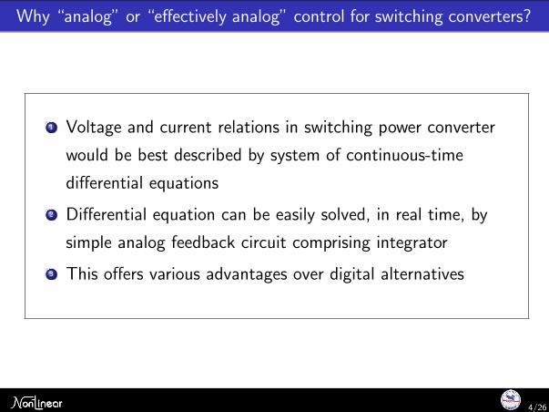
Why “analog” or “e↵ectively analog” control for switching converters?
1 Voltage and current relations in switching power converter
would be best described by system of continuous-time
di↵erential equations
2 Di↵erential equation can be easily solved, in real time, by
simple analog feedback circuit comprising integrator
3 This o↵ers various advantages over digital alternatives
4/26
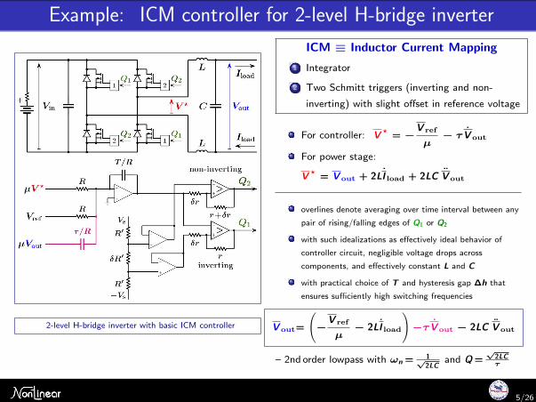
Example: ICM controller for 2-level H-bridge inverter
2-level H-bridge inverter with basic ICM controller
ICM ⌘ Inductor Current Mapping
1 Integrator
2 Two Schmitt triggers (inverting and non-
inverting) with slight o↵set in reference voltage
For controller: V?= �V ref
µ� ⌧ V out
For power stage:
V?= V out + 2LI load + 2LC V out
overlines denote averaging over time interval between any
pair of rising/falling edges of Q1 or Q2
with such idealizations as e↵ectively ideal behavior of
controller circuit, negligible voltage drops across
components, and e↵ectively constant L and C
with practical choice of T and hysteresis gap �h that
ensures su�ciently high switching frequencies
V out=
�V ref
µ� 2LI load
!�⌧ V out � 2LC V out
– 2nd order lowpass with !n = 1p2LC
and Q =p
2LC⌧
5/26
Why “analog” or “e↵ectively analog” control?
“Bare” ICM-based 3-phase 6-switch rectifier
EMI filtering with non-dissipative resonance damping
Illustrative performance examples
“E↵ectively analog” oversampled digital ICM implementation
Control and management of ICM switching behavior
6/26
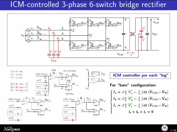
ICM-controlled 3-phase 6-switch bridge rectifier
ICM controller per each “leg”
For “bare” configuration:8>>>>>><
>>>>>>:
I a = � ⌧L V 0
a � 1LRdt�VCM�V N
�
I b = � ⌧L V 0
b � 1LRdt�VCM�V N
�
I c = � ⌧L V 0
c � 1LRdt�VCM�V N
�
Ia + Ib + Ic = 0
7/26
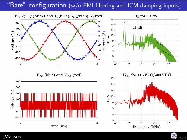
“Bare” configuration (w/o EMI filtering and ICM damping inputs)
8/26
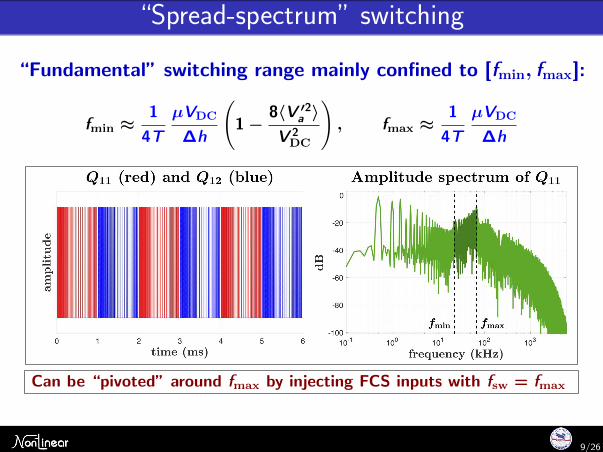
“Spread-spectrum” switching
“Fundamental” switching range mainly confined to [fmin, fmax]:
fmin ⇡1
4TµVDC
�h
1 �
8hV 02a i
V 2DC
!, fmax ⇡
1
4TµVDC
�h
Can be “pivoted” around fmax by injecting FCS inputs with fsw = fmax
9/26
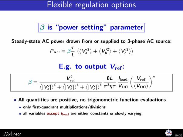
Flexible regulation options
� is “power setting” parameter
Steady-state AC power drawn from or supplied to 3-phase AC source:
PAC = �⌧
L�⌦
V 02a↵+⌦V 02
b↵+⌦V 02
c↵�
E.g. to output Vref :
� =V 2
ref⌦|V 0
a |↵2
+⌦|V 0
b |↵2
+⌦|V 0
c |↵2
8L⇡2⌘⌧
IloadVDC
✓Vref
hVDCi
◆n
All quantities are positive, no trigonometric function evaluations
only first-quadrant multiplications/divisions
all variables except Iload are either constants or slowly varying
10/26
Why “analog” or “e↵ectively analog” control?
“Bare” ICM-based 3-phase 6-switch rectifier
EMI filtering with non-dissipative resonance damping
Illustrative performance examples
“E↵ectively analog” oversampled digital ICM implementation
Control and management of ICM switching behavior
11/26
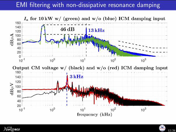
EMI filtering with non-dissipative resonance damping
12/26
Why “analog” or “e↵ectively analog” control?
“Bare” ICM-based 3-phase 6-switch rectifier
EMI filtering with non-dissipative resonance damping
Illustrative performance examples
“E↵ectively analog” oversampled digital ICM implementation
Control and management of ICM switching behavior
13/26
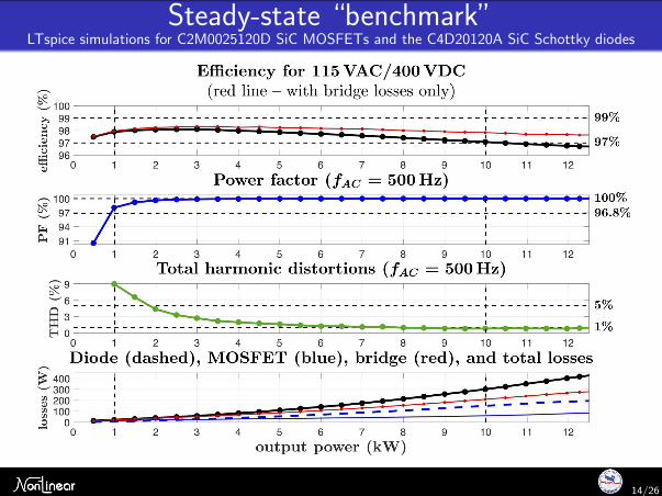
Steady-state “benchmark”LTspice simulations for C2M0025120D SiC MOSFETs and the C4D20120A SiC Schottky diodes
14/26
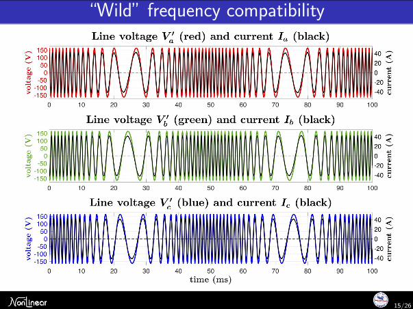
“Wild” frequency compatibility
15/26
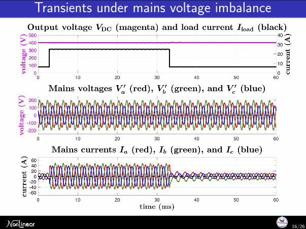
Transients under mains voltage imbalance
16/26
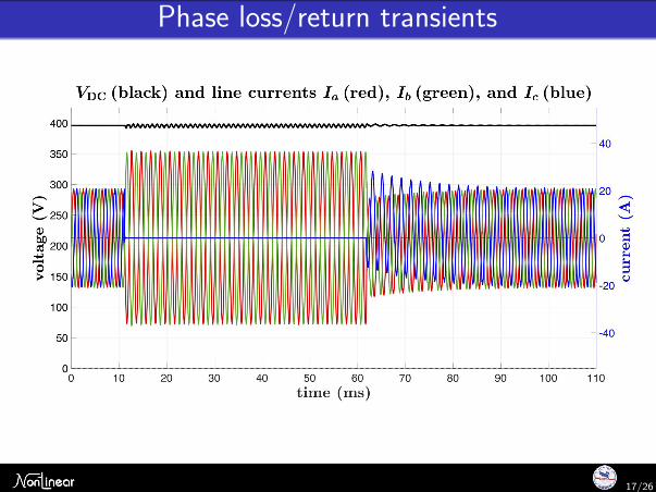
Phase loss/return transients
17/26
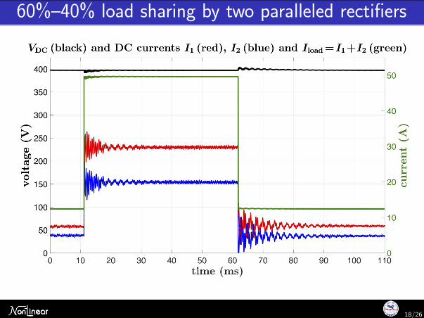
60%–40% load sharing by two paralleled rectifiers
18/26
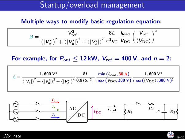
Startup/overload management
Multiple ways to modify basic regulation equation:
� =V 2
ref⌦|V 0
a |↵2
+⌦|V 0
b |↵2
+⌦|V 0
c |↵2
8L⇡2⌘⌧
IloadVDC
✓Vref
hVDCi
◆n
For example, for Pout 12 kW, Vref = 400V, and n = 2:
� =1, 600V2
⌦|V 0
a |↵2
+ h|V 0b|i
2 +⌦|V 0
c |↵2
8L0.975⇡2⌧
min (Iload, 30A)
max (VDC, 380V)
1, 600V2
max (hVDCi, 380V)2
19/26
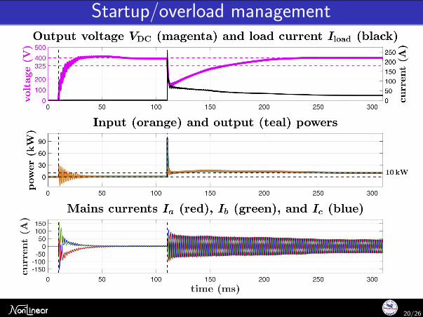
Startup/overload management
20/26
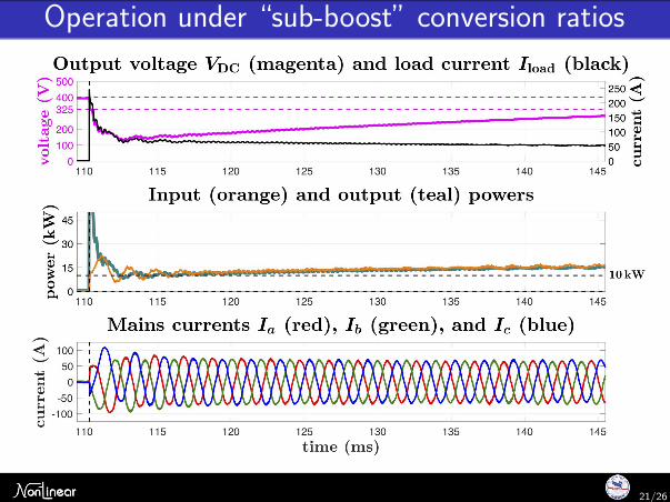
Operation under “sub-boost” conversion ratios
21/26
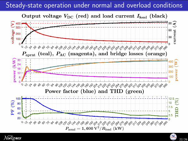
Steady-state operation under normal and overload conditions
22/26
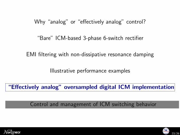
Why “analog” or “e↵ectively analog” control?
“Bare” ICM-based 3-phase 6-switch rectifier
EMI filtering with non-dissipative resonance damping
Illustrative performance examples
“E↵ectively analog” oversampled digital ICM implementation
Control and management of ICM switching behavior
23/26
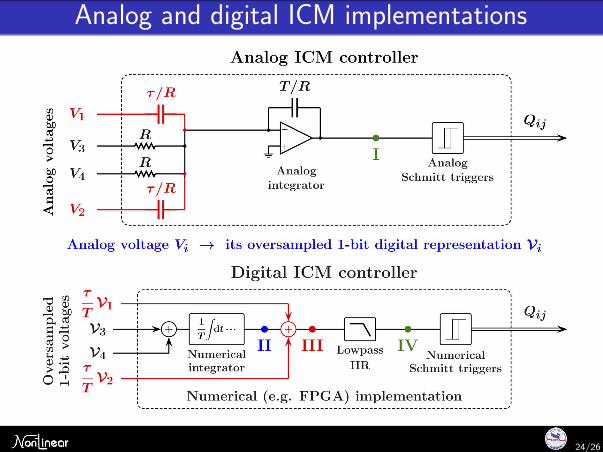
Analog and digital ICM implementations
24/26
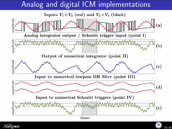
Analog and digital ICM implementations
25/26
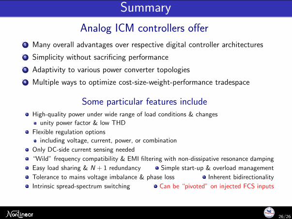
Summary
Analog ICM controllers o↵er1 Many overall advantages over respective digital controller architectures
2 Simplicity without sacrificing performance
3 Adaptivity to various power converter topologies
4 Multiple ways to optimize cost-size-weight-performance tradespace
Some particular features includeHigh-quality power under wide range of load conditions & changes
unity power factor & low THD
Flexible regulation optionsincluding voltage, current, power, or combination
Only DC-side current sensing needed
“Wild” frequency compatibility & EMI filtering with non-dissipative resonance damping
Easy load sharing & N + 1 redundancy Simple start-up & overload management
Tolerance to mains voltage imbalance & phase loss Inherent bidirectionality
Intrinsic spread-spectrum switching Can be “pivoted” on injected FCS inputs
26/26
Appendix: Control and management of ICM switching behavior
Why “analog” or “e↵ectively analog” control?
“Bare” ICM-based 3-phase 6-switch rectifier
EMI filtering with non-dissipative resonance damping
Illustrative performance examples
“E↵ectively analog” oversampled digital ICM implementation
Control and management of ICM switching behavior
27/26
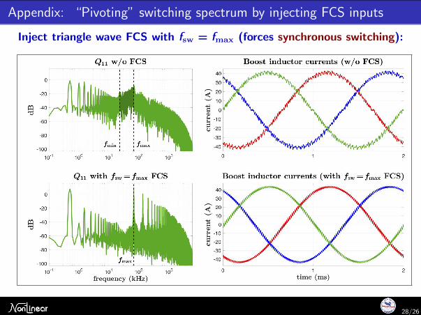
Appendix: “Pivoting” switching spectrum by injecting FCS inputs
Inject triangle wave FCS with fsw = fmax (forces synchronous switching):
28/26
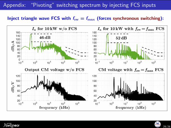
Appendix: “Pivoting” switching spectrum by injecting FCS inputs
Inject triangle wave FCS with fsw = fmax (forces synchronous switching):
29/26

“Analog” Inductor Current Mapping (ICM) control approach
Analog ICM vs digital controllers
“Holistic” high-bandwidth real-time control
incorporating flexible regulation options, startup, EMI, and overload management,
“wild” frequency compatibility, tolerance to mains voltage imbalance and/or phase loss
No analysis of various topological stages during switching cycle needed
No coordinate transformations and PLLs
No phase currents sensing
Low computational intensity for “e↵ectively analog” digital implementation
30/26