Holdings-Based and Returns-Based Style Models

June 2003

Paul D. Kaplan, Ph.D., CFADirector of ResearchMorningstar, Inc.225 West Wacker DriveChicago, IL 60606

The author thanks Robert Morioka at Morningstar for performing the holdings-based analysis andproviding the data needed to perform the returns-based analysis. The author also thanks Julie Austin andMichele Gambera of Morningstar, Barton Waring of Barclays Global Investors, Laurence Siegel of theFord Foundation, and James Knowles of York Hedge Fund Strategies for their helpful comments.

1

Introduction

Investment style is now the dominant principle used to classify, analyze, and deployequity portfolios. Investment research firms classify equity funds for ratings and otherpurposes into categories based on investment style. Institutional investors, consultants,financial investors, and individuals use investment style as a criterion for selecting funds,either to achieve diversification or make style bets. In response to the emphasis thatinvestors place on investment style, many equity mutual funds identify themselves asbeing of a certain style by using phrases such as “mid-cap growth” or “small companyvalue” in their names.

With the growing emphasis on investment style came the need for style analysis tools. Onthe one hand, because portfolio managers do not always follow their stated stylemandates (or even have stated style mandates), investors and their advisors need to beable to independently determine a portfolio’s style. On the other hand, portfolio managerswho are concerned about how investors and their advisors perceive their style need toolsto verify that they are remaining true to their intended style.

It is now a generally accepted principle that a portfolio manager who follows a particularinvestment style should be evaluated against a passive benchmark that has the same style.This leads to the twofold problem of constructing style specific benchmarks andmatching funds to the right benchmarks. Since few investment styles exactly match theconstruction rules of any single published index, it is often necessary to create custombenchmarks.1 Style analysis can be used to create custom benchmarks in the form offund-specific combinations or “portfolios” of indexes.

The same analysis can also be used to provide a more detailed description of investmentstyle than is revealed by a fund category assignment. Rather than stating that a fundbelongs in, say, the “large-cap growth” category, many equity style models assign a pairof numerical scores for size and value/growth orientation that can be plotted on an x-ygrid.2 The position of a fund’s point on the grid makes distinctions such as “core growth”and “high growth” visually apparent. If done accurately, such plots are extremely usefulin showing the distinctions between the investment styles of funds that fall into the samestyle category. This is why the ability to create such plots is a key feature of manycommercially available style analysis software packages.

Inaccurate analysis can lead to extremely inaccurate conclusions. A misleading analysisthat is easy to perform is worse than no analysis at all. Therefore, it is important for theusers of style analysis to understand how the models work and be familiar with theirlimitations before putting them into practice.

1 Quantitative active managers who use a published style index as their starting point are an

exception to this rule.

2 Sharpe [1988] introduced this type of investment style grid.

2

There are two main approaches to style analysis: holdings-based and returns-based. Therehas been much debate between proponents of these two approaches. Most of the debatehas focused on the relative accuracy of the two methods in describing a fund’s allocationamong asset classes or equity styles.3 However, no previous study compares the style plotpoints generated by the two methods. This study fills this gap by (1) developing a methodto display the style plot points generated by the two methods, and (2) comparing the styleplot points generated by the two methods over a large set of U.S. equity funds. Wehighlight where the results are similar and where they significantly differ. Where thereare significant differences, we explore some of the possible reasons. Users of styleanalysis should find this study helpful in determining which, if either, method isappropriate for their applications.

We start with an overview of holdings-based and returns-based style analysis in generaland an overview of this study.

Overview of Style Analysis

Holdings-BasedHoldings-based style analysis is a “bottom-up” approach in which the characteristics of afund over a period of time are derived from the characteristics of the securities it containsat various points in time over the period. The choice of characteristics depends on thepurpose of the analysis. If the purpose is to create a customized benchmark consisting ofa portfolio of indexes or to decompose the portfolio into a set of asset classes, the onlysecurity characteristic needed is index or asset class membership. If the purpose is todescribe a portfolio in terms of a set of quantitative style characteristics such as size andvalue/growth orientation, the prescribed characteristics of each security need to becalculated and then aggregated to the portfolio level.

Holdings-based style analysis requires two sets of data. First, we need a security databasethat contains the characteristics of each security in the investable universe of the fundsbeing analyzed. Second, we need a record of the security holdings of each fund beinganalyzed. Each database must contain the requisite data for each time period beingstudied.

The databases needed to perform holdings-based style analysis are expensive to obtainand keep up to date. Because of this, there are only a handful of investment researchfirms that have the needed datasets and perform holdings-based style analysis.

Returns-BasedSharpe [1988, 1992] introduced a low cost alternative to holdings-based style analysis,namely, returns-based style analysis. Sharpe’s approach is to regress a fund’s historicalreturns against the returns of a set of passively constructed reference portfolios, each

3 See for example Rekenthaler, Gambera, and Carlson [2002] and Buetow, Johnson, and Runkle

[2000].

3

reference portfolio representing an asset class or an investment style. The coefficients onthe reference portfolio returns are constrained to be nonnegative and sum to one so thatthey represent a long-only portfolio of passive investments. This portfolio serves as thefund’s custom benchmark.

Sharpe’s model made style analysis readily available to anyone who could obtainhistorical returns data on the portfolio being analyzed and on passive indexes. Due to theimportance of style analysis and relative inexpensiveness of returns data, Sharpe’s modelquickly became popular among institutional investors and consultants. Several firmsdeveloped software packages for both the institutional and advisor markets to performreturns-based style analysis.

Most of these software packages create plots of equity style characteristics of funds. Todo this, they first assign a point in x-y space to each reference portfolio that represents aspecific equity style, such as large-cap value. They then generate a plot point for the fundin question by taking a weighted average of the plot points of the reference portfolios,using the results of returns-based style analysis for the weights.

Overview of this Study

To generate style plot points from holdings-based analysis, we use the style model thatMorningstar introduced in 2002 to analyze stocks and equity funds and to constructequity style indexes.4 This model assigns an x-y coordinate pair to most U.S. stocks eachmonth. The x-coordinate represents the value/growth orientation and the y-coordinaterepresents size. The coordinate pairs of the stocks in a portfolio can be rolled up into theportfolio’s “centroid” by taking the asset-weighted average of the stock locations.5 Acentroid represents the overall investment style of the portfolio. The portfolio centroids ofa fund from different points in time can be averaged to measure the fund’s long-termstyle.

Using the Morningstar style model, we divide the stock universe into style specificportfolios to construct the reference portfolios for our returns-based style model. Thestyle plot points of the reference portfolios are the average portfolio centroids derivedfrom their holdings. Using the same underlying model to construct the referenceportfolios as we use for our holdings-based analysis should increase the likelihood thatthe two methods will produce similar results.

For our returns-based model, we use a standard regression model that does not constrainthe coefficients to be nonnegative. We argue that such constraints would preclude the 4 For a description of this model and some of its application, see Kaplan, Knowles, and Phillips

[2003].

5 An object’s centroid, or center of gravity, is the average location of its weight. We apply the term“centroid” to the average location of a portfolio’s asset weights on a two-dimensional grid thatrepresents investment style. Sharpe [1988] uses the term “center of gravity” in a similar fashion.

4

model from ever generating the appropriate style plot points for funds that have strongvalue or growth orientation, such as “deep value” or “high growth,” or an extreme sizebias such as “giant-cap” or “micro-cap.”6 We also argue that the model proposed byFama and French [1993, 1995, 1996], which has become popular with academicresearchers and some institutional practitioners, contains overly restrictive constraintswhen implemented as a model of fund style.7

We apply the estimated regression coefficients to the centroids of the reference portfoliosto estimate style plot points that ought to be comparable to the time-averaged centroidsobtained through holdings-based style analysis. We also construct statistical confidenceregions around the returns-based estimated centroids.

We first compare the results of the two methods for category averages. We then performour analysis on 1,909 distinct U.S. equity mutual funds from the nine U.S. diversifiedequity Morningstar Categories (“Large Value,” Large Blend,” etc.). We find that thedegree of similarity of the results of the two methods varies widely across funds. In somecases, the dissimilarity that we see is to be expected, but in other cases it is quitesurprising. To get an overall picture, we look at the overall correlation between thecentroid coordinates generated by the two methods.

We then look into possible causes for substantial differences between the results of thetwo methods. First, we see whether the degree of similarity is correlated with thegoodness-of-fit of the regression. We then consider if variation across time of styleweights could be problematic for returns-based style analysis by constructing a simplesimulation.

The Morningstar Equity Style Model

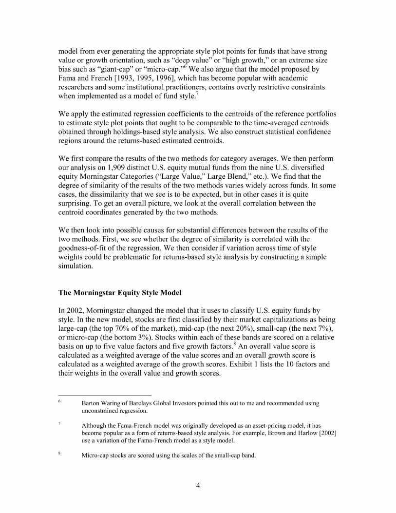
In 2002, Morningstar changed the model that it uses to classify U.S. equity funds bystyle. In the new model, stocks are first classified by their market capitalizations as beinglarge-cap (the top 70% of the market), mid-cap (the next 20%), small-cap (the next 7%),or micro-cap (the bottom 3%). Stocks within each of these bands are scored on a relativebasis on up to five value factors and five growth factors.8 An overall value score iscalculated as a weighted average of the value scores and an overall growth score iscalculated as a weighted average of the growth scores. Exhibit 1 lists the 10 factors andtheir weights in the overall value and growth scores.

6 Barton Waring of Barclays Global Investors pointed this out to me and recommended using

unconstrained regression.

7 Although the Fama-French model was originally developed as an asset-pricing model, it hasbecome popular as a form of returns-based style analysis. For example, Brown and Harlow [2002]use a variation of the Fama-French model as a style model.

8 Micro-cap stocks are scored using the scales of the small-cap band.

5

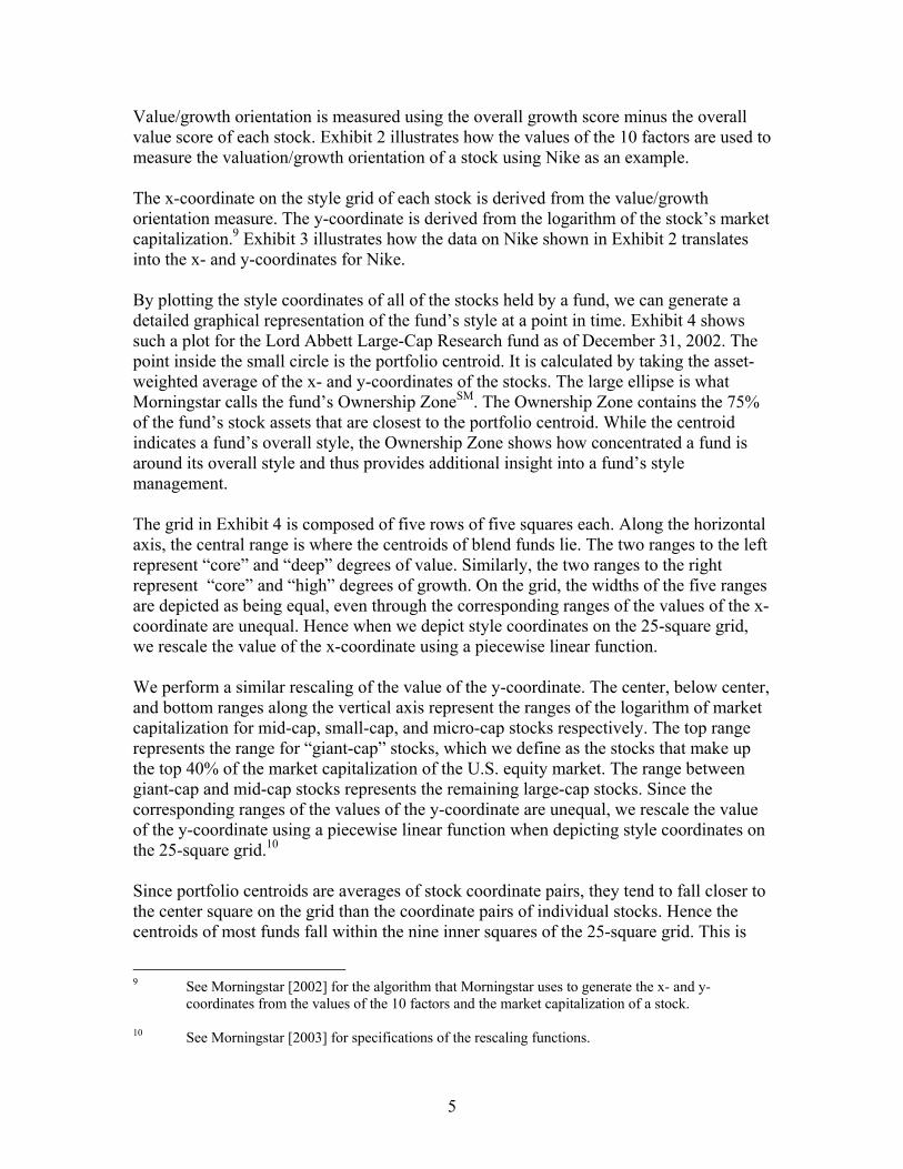
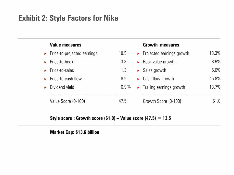
Value/growth orientation is measured using the overall growth score minus the overallvalue score of each stock. Exhibit 2 illustrates how the values of the 10 factors are used tomeasure the valuation/growth orientation of a stock using Nike as an example.

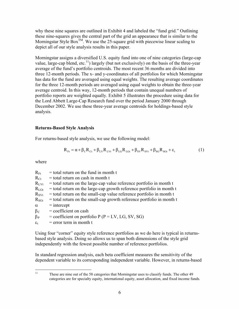
The x-coordinate on the style grid of each stock is derived from the value/growthorientation measure. The y-coordinate is derived from the logarithm of the stock’s marketcapitalization.9 Exhibit 3 illustrates how the data on Nike shown in Exhibit 2 translatesinto the x- and y-coordinates for Nike.

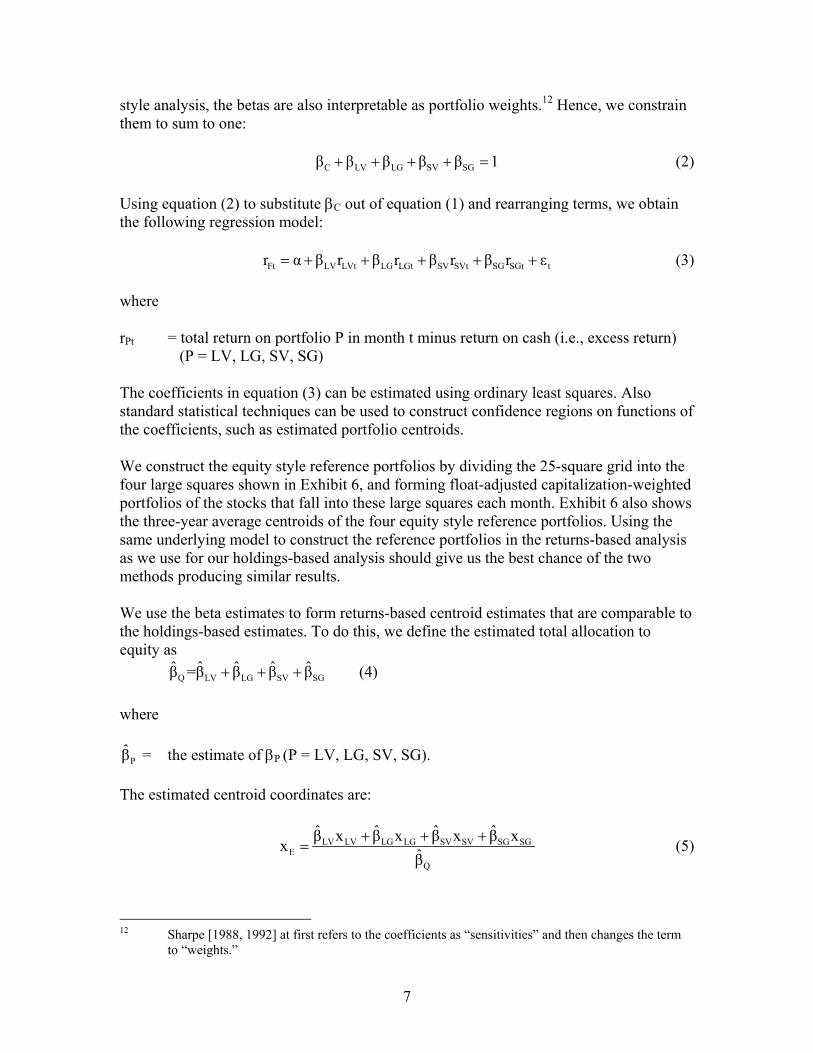
By plotting the style coordinates of all of the stocks held by a fund, we can generate adetailed graphical representation of the fund’s style at a point in time. Exhibit 4 showssuch a plot for the Lord Abbett Large-Cap Research fund as of December 31, 2002. Thepoint inside the small circle is the portfolio centroid. It is calculated by taking the asset-weighted average of the x- and y-coordinates of the stocks. The large ellipse is whatMorningstar calls the fund’s Ownership ZoneSM. The Ownership Zone contains the 75%of the fund’s stock assets that are closest to the portfolio centroid. While the centroidindicates a fund’s overall style, the Ownership Zone shows how concentrated a fund isaround its overall style and thus provides additional insight into a fund’s stylemanagement.

The grid in Exhibit 4 is composed of five rows of five squares each. Along the horizontalaxis, the central range is where the centroids of blend funds lie. The two ranges to the leftrepresent “core” and “deep” degrees of value. Similarly, the two ranges to the rightrepresent “core” and “high” degrees of growth. On the grid, the widths of the five rangesare depicted as being equal, even through the corresponding ranges of the values of the x-coordinate are unequal. Hence when we depict style coordinates on the 25-square grid,we rescale the value of the x-coordinate using a piecewise linear function.

We perform a similar rescaling of the value of the y-coordinate. The center, below center,and bottom ranges along the vertical axis represent the ranges of the logarithm of marketcapitalization for mid-cap, small-cap, and micro-cap stocks respectively. The top rangerepresents the range for “giant-cap” stocks, which we define as the stocks that make upthe top 40% of the market capitalization of the U.S. equity market. The range betweengiant-cap and mid-cap stocks represents the remaining large-cap stocks. Since thecorresponding ranges of the values of the y-coordinate are unequal, we rescale the valueof the y-coordinate using a piecewise linear function when depicting style coordinates onthe 25-square grid.10

Since portfolio centroids are averages of stock coordinate pairs, they tend to fall closer tothe center square on the grid than the coordinate pairs of individual stocks. Hence thecentroids of most funds fall within the nine inner squares of the 25-square grid. This is

9 See Morningstar [2002] for the algorithm that Morningstar uses to generate the x- and y-

coordinates from the values of the 10 factors and the market capitalization of a stock.

10 See Morningstar [2003] for specifications of the rescaling functions.

6

why these nine squares are outlined in Exhibit 4 and labeled the “fund grid.” Outliningthese nine-squares gives the central part of the grid an appearance that is similar to theMorningstar Style BoxTM. We use the 25-square grid with piecewise linear scaling todepict all of our style analysis results in this paper.

Morningstar assigns a diversified U.S. equity fund into one of nine categories (large-capvalue, large-cap blend, etc.11) largely (but not exclusively) on the basis of the three-yearaverage of the fund’s portfolio centroids. The most recent 36 months are divided intothree 12-month periods. The x- and y-coordinates of all portfolios for which Morningstarhas data for the fund are averaged using equal weights. The resulting average coordinatesfor the three 12-month periods are averaged using equal weights to obtain the three-yearaverage centroid. In this way, 12-month periods that contain unequal numbers ofportfolio reports are weighted equally. Exhibit 5 illustrates the procedure using data forthe Lord Abbett Large-Cap Research fund over the period January 2000 throughDecember 2002. We use these three-year average centroids for holdings-based styleanalysis.

Returns-Based Style Analysis

For returns-based style analysis, we use the following model:

Ft C Ct LV LVt LG LGt SV SVt SG SGt tR α β R β R β R β R β R ε= + + + + + + (1)

where

RFt = total return on the fund in month tRCt = total return on cash in month tRLVt = total return on the large-cap value reference portfolio in month tRLGt = total return on the large-cap growth reference portfolio in month tRSVt = total return on the small-cap value reference portfolio in month tRSGt = total return on the small-cap growth reference portfolio in month tα = interceptβC = coefficient on cashβP = coefficient on portfolio P (P = LV, LG, SV, SG)εt = error term in month t

Using four “corner” equity style reference portfolios as we do here is typical in returns-based style analysis. Doing so allows us to span both dimensions of the style gridindependently with the fewest possible number of reference portfolios.

In standard regression analysis, each beta coefficient measures the sensitivity of thedependent variable to its corresponding independent variable. However, in returns-based

11 These are nine out of the 58 categories that Morningstar uses to classify funds. The other 49

categories are for specialty equity, international equity, asset allocation, and fixed income funds.

7

style analysis, the betas are also interpretable as portfolio weights.12 Hence, we constrainthem to sum to one:

C LV LG SV SGβ β β β β 1+ + + + = (2)

Using equation (2) to substitute βC out of equation (1) and rearranging terms, we obtainthe following regression model:

Ft LV LVt LG LGt SV SVt SG SGt tr α β r β r β r β r ε= + + + + + (3)

where

rPt = total return on portfolio P in month t minus return on cash (i.e., excess return) (P = LV, LG, SV, SG)

The coefficients in equation (3) can be estimated using ordinary least squares. Alsostandard statistical techniques can be used to construct confidence regions on functions ofthe coefficients, such as estimated portfolio centroids.

We construct the equity style reference portfolios by dividing the 25-square grid into thefour large squares shown in Exhibit 6, and forming float-adjusted capitalization-weightedportfolios of the stocks that fall into these large squares each month. Exhibit 6 also showsthe three-year average centroids of the four equity style reference portfolios. Using thesame underlying model to construct the reference portfolios in the returns-based analysisas we use for our holdings-based analysis should give us the best chance of the twomethods producing similar results.

We use the beta estimates to form returns-based centroid estimates that are comparable tothe holdings-based estimates. To do this, we define the estimated total allocation toequity as

Q LV LG SV SGˆ ˆ ˆ ˆ ˆβ =β β β β+ + + (4)

where

Pβ = the estimate of βP (P = LV, LG, SV, SG).

The estimated centroid coordinates are:

LV LV LG LG SV SV SG SGE

Q

ˆ ˆ ˆ ˆβ x β x β x β xxβ

+ + += (5)

12 Sharpe [1988, 1992] at first refers to the coefficients as “sensitivities” and then changes the term

to “weights.”

8

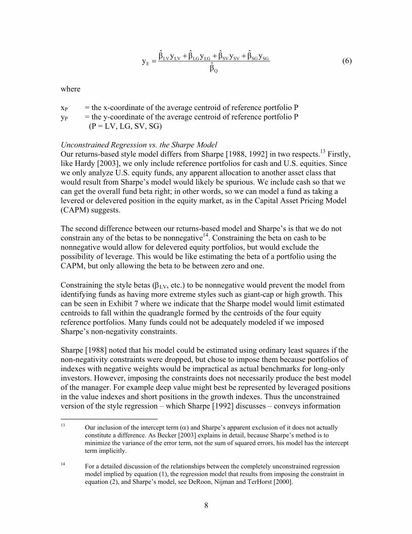
LV LV LG LG SV SV SG SGE

Q

ˆ ˆ ˆ ˆβ y β y β y β yyβ

+ + += (6)

where

xP = the x-coordinate of the average centroid of reference portfolio PyP = the y-coordinate of the average centroid of reference portfolio P

(P = LV, LG, SV, SG)

Unconstrained Regression vs. the Sharpe ModelOur returns-based style model differs from Sharpe [1988, 1992] in two respects.13 Firstly,like Hardy [2003], we only include reference portfolios for cash and U.S. equities. Sincewe only analyze U.S. equity funds, any apparent allocation to another asset class thatwould result from Sharpe’s model would likely be spurious. We include cash so that wecan get the overall fund beta right; in other words, so we can model a fund as taking alevered or delevered position in the equity market, as in the Capital Asset Pricing Model(CAPM) suggests.

The second difference between our returns-based model and Sharpe’s is that we do notconstrain any of the betas to be nonnegative14. Constraining the beta on cash to benonnegative would allow for delevered equity portfolios, but would exclude thepossibility of leverage. This would be like estimating the beta of a portfolio using theCAPM, but only allowing the beta to be between zero and one.

Constraining the style betas (βLV, etc.) to be nonnegative would prevent the model fromidentifying funds as having more extreme styles such as giant-cap or high growth. Thiscan be seen in Exhibit 7 where we indicate that the Sharpe model would limit estimatedcentroids to fall within the quadrangle formed by the centroids of the four equityreference portfolios. Many funds could not be adequately modeled if we imposedSharpe’s non-negativity constraints.

Sharpe [1988] noted that his model could be estimated using ordinary least squares if thenon-negativity constraints were dropped, but chose to impose them because portfolios ofindexes with negative weights would be impractical as actual benchmarks for long-onlyinvestors. However, imposing the constraints does not necessarily produce the best modelof the manager. For example deep value might best be represented by leveraged positionsin the value indexes and short positions in the growth indexes. Thus the unconstrainedversion of the style regression – which Sharpe [1992] discusses – conveys information 13 Our inclusion of the intercept term (α) and Sharpe’s apparent exclusion of it does not actually

constitute a difference. As Becker [2003] explains in detail, because Sharpe’s method is tominimize the variance of the error term, not the sum of squared errors, his model has the interceptterm implicitly.

14 For a detailed discussion of the relationships between the completely unconstrained regressionmodel implied by equation (1), the regression model that results from imposing the constraint inequation (2), and Sharpe’s model, see DeRoon, Nijman and TerHorst [2000].

9

about the manager that is not in the constrained model. This information is manifested onthe style grid when the estimated centroid falls outside of the quadrangle in Exhibit 7.Also, if the constraints are binding, the goodness-of-fit is necessarily better with theunconstrained regression. Furthermore, if a coefficient is constrained to be zero, thecorresponding index return series could be correlated with the error term. This isproblematic because the error is supposed to represent security selection effects, which inprinciple ought to be statistically independent of style effects. For all of these reasons, weadopt the unconstrained approach to style analysis in this paper.

Unconstrained Regression vs. the Fama-French ModelThe model introduced by Fama and French [1993, 1995, 1996] is often used in academicresearch as a form of returns-based style analysis for U.S. equity portfolios. Using ourreference portfolios, the Fama-French model can be implemented as follows:15

( ) ( )Ft Q Mt x LVt SVt LGt SGt y SVt SGt LVt LGt tr α β r γ r r r r γ r r r r ε= + + + − − + + − − + (7)

where

rMt = total return on the equity market portfolio minus return on cash in month tγx = a parameter that measures the fund’s value/growth orientation γy = a parameter that measures the fund’s size orientation

and all other symbols are as they are defined previously.

Suppose that the equity market portfolio were a fixed-weight combination of our fourequity style reference portfolios.16 We could write

Mt LV LVt LG LGt SV SVt SG SGtr w r w r w r w r= + + + (8)

where

wP = the market weight of reference portfolio P.

By definition,

LV LG SV SGw w w w 1+ + + = (9)

15 Fama and French decompose the market into six portfolios by including a “neutral” category

between value (high book-to-market) and growth (low book-to-market.) They include the neutralportfolios in the size factor, but exclude them from the value/growth orientation factor. Since wedo carve out a neutral territory like this, we do not do this in our interpretation of their model.

16 Regressing the excess return on the float-adjusted capitalization-weighted composite of the fourreference portfolios on the excess returns of four reference portfolios over the 36-month periodJanuary 2000 – December 2002 yields an R-squared value of 99.8%. So the fixed-weightassumption is a reasonable one for our purpose here.

10

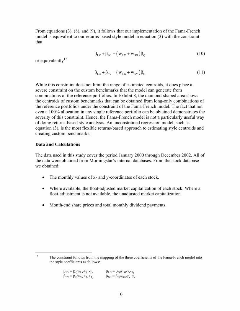
From equations (3), (8), and (9), it follows that our implementation of the Fama-Frenchmodel is equivalent to our returns-based style model in equation (3) with the constraintthat

( )LV SG LV SG Qβ β w w β+ = + (10)or equivalently17

( )LG SV LG SV Qβ β w w β+ = + (11)

While this constraint does not limit the range of estimated centroids, it does place asevere constraint on the custom benchmarks that the model can generate fromcombinations of the reference portfolios. In Exhibit 8, the diamond-shaped area showsthe centroids of custom benchmarks that can be obtained from long-only combinations ofthe reference portfolios under the constraint of the Fama-French model. The fact that noteven a 100% allocation in any single reference portfolio can be obtained demonstrates theseverity of this constraint. Hence, the Fama-French model is not a particularly useful wayof doing returns-based style analysis. An unconstrained regression model, such asequation (3), is the most flexible returns-based approach to estimating style centroids andcreating custom benchmarks.

Data and Calculations

The data used in this study cover the period January 2000 through December 2002. All ofthe data were obtained from Morningstar’s internal databases. From the stock databasewe obtained:

• The monthly values of x- and y-coordinates of each stock.

• Where available, the float-adjusted market capitalization of each stock. Where afloat-adjustment is not available, the unadjusted market capitalization.

• Month-end share prices and total monthly dividend payments.

17 The constraint follows from the mapping of the three coefficients of the Fama-French model into

the style coefficients as follows:

βLV = βQwLV+γx-γy βLG = βQwLG-γx-γy

βSV = βQwSV+γx+γy βSG = βQwSG-γx+γy

11

From the fund database we obtained the following data on diversified U.S. equity funds:

• The category of each fund as of February 2003.

• Month-end security identifiers and dollars invested in each security of each fund,to the extent that fund companies reported them to Morningstar over the 2000-2002 period.18

• Monthly total returns on each share class of each fund that has a complete returnhistory over the 2000-2002 period.

We found the requisite data on 1,909 “distinct” funds (that is, counting multiple shareclasses as one fund). Exhibit 9 shows the number of distinct funds in each of the nineMorningstar Categories of U.S. diversified equity funds.

From the x- and y-coordinates of the stocks and the holdings data on the funds, wecalculate the three-year average centroids of the funds. The category average centroidsare the simple averages of the three-year average centroids of all funds within eachcategory.

From the share price and dividend data, we calculate the monthly total return of eachstock. Based on each stock’s x- and y-coordinates each month, we place each stock eachmonth into one of the four reference portfolios. For each month we calculate the float-adjusted capitalization weighted total return and centroid. We average the monthlycentroid coordinates to form the reference portfolio centroids shown in Exhibit 6.

For funds with multiple share classes, we calculate the simple average of the total returnsof the various share classes for each month to obtain a single time-series of total returnsfor each distinct fund. Category average returns are the simple averages of the resultingreturns on all distinct funds within each category.

We subtract the return on cash19 each month from the total returns on the funds, thecategory averages, and the reference portfolios, and then estimate the parameters ofequation (3) for each fund and category average using ordinary least squares regression.Using equations (4), (5), and (6) we calculate the returns-based centroid estimate of eachfund and category average. Using the method described in the Appendix, we calculate a95% confidence region around each estimated centroid.

18 Nearly all funds report portfolio holdings semiannually to Morningstar since they have to report

this information to their shareholders anyway in accordance with SEC regulations. Most fundcompanies, including 71 out of the largest 75, go beyond this, reporting portfolio holdings toMorningstar quarterly or monthly.

19 Returns on cash are calculated by Morningstar from yields on 90-day Treasury bills.

12

Results

Category AveragesWe first compare the results of holdings-based and returns-based centroid estimates forcategory averages. Exhibit 10 shows the R-squared values for each of the nine categoryaverage regressions. They are all quite high, the lowest being 94.8%.

Exhibit 11 shows the estimated centroids and confidence regions for the nine categoryaverages. In all cases, the estimated centroids fall in the right general area of the grid.However, the returns-based estimates for mid-cap growth and small-cap growth fall intothe extreme area of the grid. This happens because in these cases, the estimatedcoefficient on the large-cap value reference portfolio is negative in sign and large inmagnitude20. This raises questions about the reliability of the returns-based method.

The confidence regions shown in Exhibit 11 are much larger for mid-cap growth, small-cap blend, and small-cap growth than they are for the other category averages, eventhough the R-squared values are not much lower.21 This is because in these regressions,the volatility of the error term, as measured by the standard error of regression, issignificantly larger than in the other regressions. Also, the total estimated allocation toequity – Qβ as defined by equation (4) – is lower in these regressions than in the otherregressions (81-84% as opposed to about 100%)22. This lowers the statistical significanceof the point estimates and hence enlarges the confidence regions.23

Individual FundsAt the individual fund level, there are many cases in which the results of holdings-basedanalysis and returns-based analysis can be quite similar. As shown in Exhibit 12, this isthe case for some very well known funds.24 However, there can also be substantialdifferences as shown in Exhibit 13 .25

20 -19% and -32% respectively.

21 In ordinary x-y space, the confidence regions would be perfectly elliptical. However, because ofthe piecewise linear rescaling that we use when plotting style coordinates on the 25-square grid,the ellipses are distorted when they cross two or more squares.

22 Standard error and beta estimates on category average regressions are available from the author.

23 See equation (A.13) in the appendix.

24 Ben Dor, Jagannathan, and Meier [2003] also present returns-based results for Vanguard Growthand Income as well as four other funds to demonstrate the value of returns-based style analysis.For all five of their sample funds, the results of returns-based and holdings-based analysis aresimilar in our analysis.

25 The regression for Legg Mason Value (Exhibit 12) and Van Kampen American Value (Exhibit 13)have similar R-squared values and standard errors of regression. The difference in the sizes oftheir respective confidence regions is due to a large difference in their respective estimatedallocations to equity: 129% for Legg Mason vs. 64% for Van Kampen.

13

Returns-based style analysis can be useful for funds that get their exposure to an assetclass by taking long positions in index futures rather than by holding the underlyingsecurities outright. A good example of this is the PIMCO StocksPlus fund. This fundtakes long positions in S&P 500 futures contracts, which it fully collateralizes with fixedincome investments. As shown in Exhibit 14, returns-based style analysis correctlymodels the portfolio as having nearly the same style characteristics as the S&P 500.

However, returns-based analysis does not work well with all non-conventionalinvestment practices. For example, the manager of Needham Growth fund regularly tookshort positions in high growth stocks and growth exchange traded funds over our periodof study.26 This should have given the fund’s return pattern a more moderate growth tiltthan would be evident from its direct holdings. We would expect the results of returns-based style analysis to reflect this. However, as shown in Exhibit 15, the opposite seemsto occur. As we discuss later, this could be due to a poor goodness-of-fit of theregression,27 or the time variation in style exposures, or a combination of both.

Exhibit 16 presents the averages of the R-squared values from the individual fundregressions by category. For large-cap funds, average R-squared value is over 90%. Formid-cap and small-cap funds, it is a bit lower at about 85%. This would suggest that thestyle regressions do a reasonably good job of describing the return patterns – although notnecessarily the actual style exposures – of funds.

However, as we saw with some particular funds, high values of R-squared may or maynot correspond with good estimates of style characteristics. Exhibit 17 shows that forlarge-cap value funds, holdings-based and returns-based estimated centroids both areconcentrated in the large-cap value area of the style grid.28 However, large-cap value isthe only one of the nine diversified U.S. equity fund categories for which this holds. Forexample, as Exhibit 18 shows, the picture is very different for mid-cap blend funds.While the holdings-based centroid estimates are concentrated in the mid-cap blendsquare, the returns-based estimates are scattered across the grid. This occurs even thoughthe rescaled29 estimated coordinates between the two methods are more correlated formid-cap blend funds than they are for large-cap value funds. Exhibit 19 shows the resultsfor small-cap growth funds where the correlation between the rescaled y-coordinatesfrom the two methods breaks down completely.

26 See Sweeney [2003] for a description of then fund manager Peter Trapp’s investment practices.

Trapp left Needham in 2003 to enter the hedge-fund business.

27 A relatively low R-squared value and a very high standard error of regression suggest that areturns-based model might give poor representation of this fund.

28 Since Morningstar used the three-year average holdings-based centroid as the main criterion forclassifying diversified U.S. equity funds, the concentrations seen on the holdings-based side ofExhibits 17, 18, and 19 are mainly by construction.

29 I.e., rescaled as described in Morningstar [2003].

14

Exhibits 20 and 21 show that while overall, there is a high correlation between holdings-based and returns-based rescaled centroid coordinates, the relationship does not hold upfor many funds, especially for the y-coordinate of mid-cap and small-cap funds.

Reasons Why Returns-Based Style Analysis Might Break Down

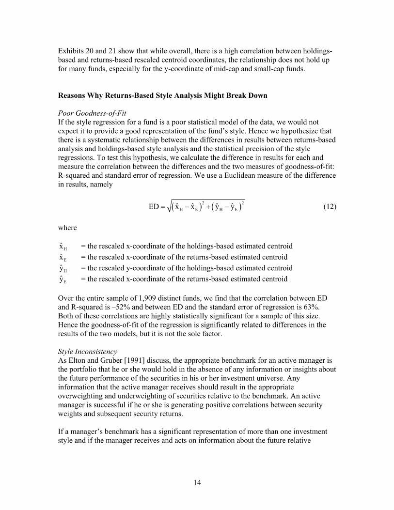
Poor Goodness-of-FitIf the style regression for a fund is a poor statistical model of the data, we would notexpect it to provide a good representation of the fund’s style. Hence we hypothesize thatthere is a systematic relationship between the differences in results between returns-basedanalysis and holdings-based style analysis and the statistical precision of the styleregressions. To test this hypothesis, we calculate the difference in results for each andmeasure the correlation between the differences and the two measures of goodness-of-fit:R-squared and standard error of regression. We use a Euclidean measure of the differencein results, namely

( ) ( )2 2H E H Eˆ ˆ ˆ ˆED x x y y= − + − (12)

where

Hx = the rescaled x-coordinate of the holdings-based estimated centroid

Ex = the rescaled x-coordinate of the returns-based estimated centroid

Hy = the rescaled y-coordinate of the holdings-based estimated centroid

Ey = the rescaled x-coordinate of the returns-based estimated centroid

Over the entire sample of 1,909 distinct funds, we find that the correlation between EDand R-squared is –52% and between ED and the standard error of regression is 63%.Both of these correlations are highly statistically significant for a sample of this size.Hence the goodness-of-fit of the regression is significantly related to differences in theresults of the two models, but it is not the sole factor.

Style InconsistencyAs Elton and Gruber [1991] discuss, the appropriate benchmark for an active manager isthe portfolio that he or she would hold in the absence of any information or insights aboutthe future performance of the securities in his or her investment universe. Anyinformation that the active manager receives should result in the appropriateoverweighting and underweighting of securities relative to the benchmark. An activemanager is successful if he or she is generating positive correlations between securityweights and subsequent security returns.

If a manager’s benchmark has a significant representation of more than one investmentstyle and if the manager receives and acts on information about the future relative

15

performance of those styles, the manager’s style mix should deviate from thebenchmark’s over time, resulting in style inconsistency.30

To see what implications such style inconsistency might have for returns-based styleanalysis, we construct a synthetic series of fund returns in which the manager picks oneof four mixes of the reference portfolios. We assume that the manager has perfectforesight at the end of each month as to which of the four reference portfolio will havethe best performance in the following month and chooses the mix with the highestallocation to the best performing reference portfolio. The mixes are constructed so thatthe average allocation is 25% in each of the four reference portfolios. Exhibit 22 showsthe four mixes and how they are constructed.

Exhibit 23 presents the results of the style regression for the synthetic portfolio. At95.3%, the R-squared value would indicate a very good fit. The other regression statisticsconfirm this. Yet, the estimated coefficients are quite different than the actual averageallocations of 25% to each reference portfolio. From this we conclude that the results ofreturns-based style analysis can be quite misleading if there is a significant amount ofstyle inconsistency over the period of study.31 The extent to which equity funds are styleinconsistent32 and the actual effects of style inconsistency on the results of returns-basedstyle analysis are empirical questions that need further investigation.

Summary and Conclusions

Holdings-based and returns-based models are both used to describe investment style. Inthis study, we present a framework that allows us to do a systematic comparison of theresults of the two methods and apply it to a large set of U.S. equity mutual funds.

For holdings-based style analysis, we use Morningstar’s new 10 factor style model. TheMorningstar model allows us to classify stocks, calculate style centroids and ownershipzones for funds, and create reference portfolios for returns-based style analysis.

30 As described here, style inconsistency should result in superior performance. Brown and Harlow

[2002] claim to show that style inconsistency has been detrimental to performance. However, theyuse the R-squared from a Fama-French type model and tracking error against published stylebenchmarks as measures of style consistency rather than any measure based on actual styleexposures. As we show below, goodness-of-fit statistics can be poor indicators of styleconsistency.

31 Practitioners of returns-based style analysis often use rolling overlapping periods to estimate styledrift. However, this approach does not address the estimation problems caused by styleinconsistency shown here. A more promising approach would be to embed the time variation ofthe style weights directly into the model as Spiegel, Mamaysky, and Zhang [2003] do in a singlefactor model.

32 A similar problem occurs if the performance effects of a fund’s active security selection arecorrelated with the returns on the style reference portfolios.

16

For returns-based style analysis, we use an unconstrained linear regression model. Weargue that the popular Sharpe and Fama-French returns-based models place severe andunrealistic constraints on reference portfolio weights. Our unconstrained model allows usto estimate style centroids and confidence regions in a straightforward manner.

We find that high R-squared values do not necessarily mean that returns-based stylecentroid estimates are reliable. Even when modeling portfolios of funds that all belong tothe same style category, we find that the returns-based method can give extreme resultswith large confidence intervals, although the R-squared values are high.

We find that holdings-based and returns-based results are similar for many funds butdiffer substantially for others. Hence, holdings-based and returns-based analysis couldlead to very different style classifications for many funds. We explore whether goodness-of-fit statistics for the style regressions can systematically explain the extent of thedifferences. We find that they are significantly related to differences in the results of thetwo models, but the goodness-of-fit of the style regression cannot be regarded as the solefactor leading to the differences. Other possible sources of differences include styleinconsistency (which we demonstrate by a simulation) and correlation between selectionand style effects. These possibilities require further investigation.

If a fund’s portfolio is primarily composed of direct stock holdings, holdings-basedanalysis should be the primary means of assessing investment style. In the absence ofsuch information, and under the right conditions, returns-based style analysis can be usedto estimate investment style. Users of returns-based style analysis need to be aware of theconditions in which it produces inaccurate results. Users of all models need to keep inmind that quantitative techniques can complement, but never replace, qualitativeknowledge of a fund’s style and strategy.

17

Appendix: Confidence Regions for Estimate Style Centroids

Our unconstrained style regression equation is

Ft LV LVt LG LGt SV SVt SG SGt tr α β r β r β r β r ε= + + + + + (A.1)

Let

qt = Excess return on fund in period t minus its time-series averagezt = Vector of excess returns on the reference portfolios in period t minus the vector of

their time-series averagesβ = Vector of coefficients on the reference portfoliosσ2 = Var[εt]

We can rewrite equation (A.1) as follows:

t t tq β ' z ε= + (A.2)

Let

T = Number of time-series observationsq = T-element vector of values of qt

Z = T × 4 matrix of the values of zt

The ordinary least squares estimators of β and σ2 are

( ) 1β Z'Z Z'q−= (A.3)and

2 ˆ ˆε 'εσT 5

=−

(A.4)

where

ˆε q Zβ= − (A.5)

The estimated variance-covariance matrix of β is

( ) 12ˆ σ Z'Z −Σ = (A.6)

18

Let

xR = 4-element vector of x-coordinates of the centroids of the reference portfoliosyR = 4-element vector of y-coordinates of the centroids of the reference portfolios

The returns-based estimate of the centroid coordinates are

RE

Q

ˆx 'βxβ

= (A.7)

RE

Q

ˆy 'βyβ

= (A.8)

where

Q LV LG SV SGˆ ˆ ˆ ˆ ˆβ β β β β= + + + (A.9)

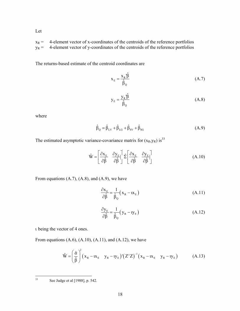
The estimated asymptotic variance-covariance matrix for (xR,yR) is33

'

E E E Ex y x yˆ ˆW ˆ ˆ ˆ ˆβ β β β ∂ ∂ ∂ ∂

= Σ ∂ ∂ ∂ ∂

(A.10)

From equations (A.7), (A.8), and (A.9), we have

( )ER E

Q

x 1 x ιxˆ ˆβ β∂

= −∂

(A.11)

( )ER E

Q

y 1 y ιyˆ ˆβ β∂

= −∂

(A.12)

ι being the vector of 4 ones.

From equations (A.6), (A.10), (A.11), and (A.12), we have

( ) ( ) ( )2

1R E R E R E R E

σW x ιx y ιy ' Z 'Z x ιx y ιyβ

− = − − − −

(A.13)

33 See Judge et al [1988], p. 542.

19

If x and y are the true values of the x- and y-coordinates, asymptotically, the quantity

'E E1

E E

x x x xW

y y y y−− −

− −

is a random variable with a chi-squared distribution with 2 degrees of freedom. Let

( )22χ p = the critical value for a chi-squared distribution with 2 degrees of freedom

for a 100p percent confidence region (5.99 for 95% confidence region)

The 100p percent confidence region around (xE, yE) is the set of coordinate pairs (x,y)that satisfies

( )'

E E1 22

E E

x x x xW χ p

y y y y−− −

≤ − − (A.14)

20

References

Becker, Thomas R., “Exploring the Mathematical Basis of Returns-Based StyleAnalysis,” in Handbook of Equity Style Management, Third Edition, T. Daniel Cogginand Frank J. Fabozzi, eds., John Wiley & Sons, 2003.

Ben Dor, Arik, Ravi Javannathan, and Iwan Meier, “Understanding Mutual Fund andHedge Fund Styles Using Return-Based Style Analysis,” Journal of InvestmentManagement, 2003, vol.1, no 1., pp. 94-134.

Brown, Keith C. and W. V. Harlow, “Staying the Course: The Impact of Investment StyleConsistency on Mutual Fund Performance,” March 2002. Available atwww.mccombs.utexas.edu/~brownk/Research/styleconsistent-wp.pdf.

Buetow, Gerald W., Jr., Robert R. Johnson, and David E. Runkle in “The Inconsistencyof Returns-Based Style Analysis,” Journal of Portfolio Management, Spring 2000.

DeRoon, Frans A., Theo E. Nijman, and Jenke R. Terhorst, “Evaluating Style Analysis,”March 2000, Erasmus Research Institute of Management, Erasmus University, discussionpaper no. 18. Available at www.eur.nl/WebDOC/doc/erim/erimrs20000525115250.pdf.

Elton, Edwin J. and Martin J. Gruber, “Differential Information and Timing Ability,”Journal of Banking and Finance, 1991, 15:117-131.

Fama, Eugene and Kenneth French, “Common Risk Factors in the Returns on Stocks andBonds,” Journal of Financial Economics, 1993, 33:3-56.

Fama, Eugene and Kenneth French, “Size and Book-to-Market Factors in Earnings andReturns,” Journal of Finance, 1995, 50:131-155.

Fama, Eugene and Kenneth French, “Multifactor Explanations of Asset PricingAnomalies,” Journal of Finance, 1996, 51:55-84.

Hardy, Stephen R., “Style Analysis: A Ten-Year Retrospective and Commentary,” inHandbook of Equity Style Management, Third Edition, T. Daniel Coggin and Frank J.Fabozzi, eds., John Wiley & Sons, 2003.

Judge, George G., R. Carter Hill, William E. Griffiths, Helmut Lütkepohl, and Tsoung-Chao Lee, Introduction to the Theory and Practice of Econometrics, Second Edition,John Wiley & Sons, 1988.

Kaplan, Paul D., James A. Knowles, and Don Phillips, “More Depth and Breadth than theStyle Box: The Morningstar Lens,” in Handbook of Equity Style Management, ThirdEdition, T. Daniel Coggin and Frank J. Fabozzi, eds., John Wiley & Sons, 2003.

21

“The New Morningstar Style Box Methodology,” Morningstar research paper, May 2002.Available at datalab.morningstar.com.

“The Elements of Morningstar Fund Style,” Morningstar, 2003. Available from theauthor.

Rekenthaler, John, Michele Gambera, and Joshua Charlson, “Estimating Portfolio Style:A Comparative Study of Portfolio-Based Fundamental Analysis and Returns-Based StyleAnalysis,” Morningstar research paper, 2002. Available at datalab.morningstar.com.

Spiegel, Matthew, Harry Marmaysky, and Hong Zhang, “Estimating the Dynamics ofMutual Fund Alphas and Betas,” March 2003, Yale International Center for Financeworking paper no. 03-03. Available at ssrn.com/abstract_id=389740.

Sweeney, Bradley, “Morningstar’s Take,” Needham Growth, www.morningstar.com,April 2003.

Sharpe, William F., “Determining a Fund’s Effective Asset Mix,” InvestmentManagement Review, December 1988, pp. 59-69.

Sharpe, William F., “Asset Allocation: Management Style and PerformanceMeasurement,” Journal of Portfolio Management, Winter 1992, pp. 7-19.

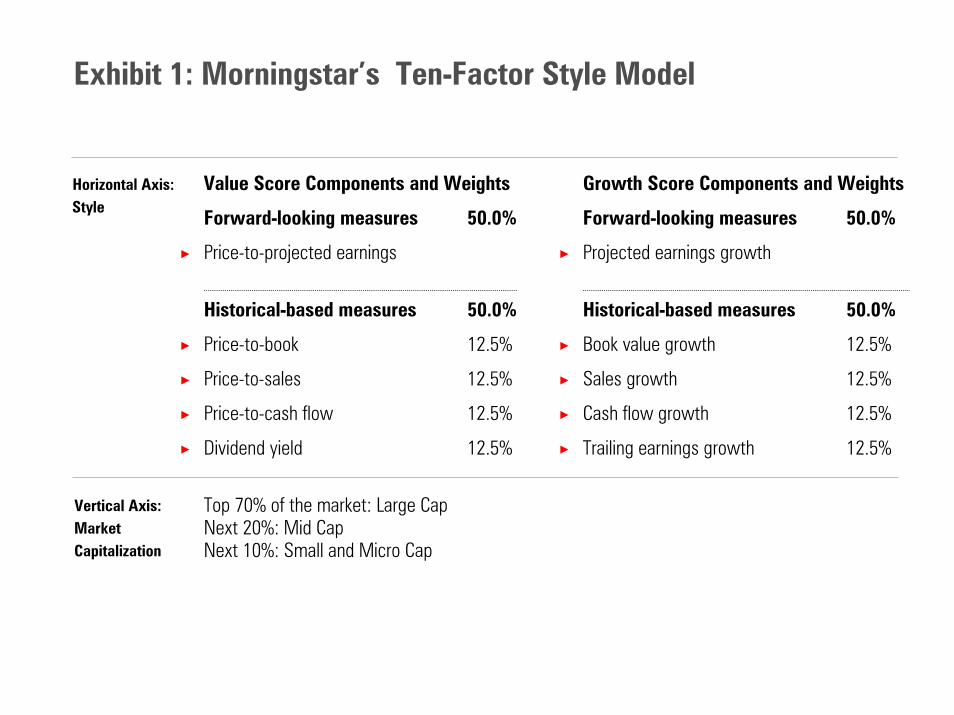
Exhibit 1: Morningstar’s Ten-Factor Style Model

Horizontal Axis:Style

Value Score Components and Weights

Forward-looking measures 50.0%

× Price-to-projected earnings

Historical-based measures 50.0%

× Price-to-book 12.5%

× Price-to-sales 12.5%

× Price-to-cash flow 12.5%

× Dividend yield 12.5%

Top 70% of the market: Large CapNext 20%: Mid CapNext 10%: Small and Micro Cap

Growth Score Components and Weights

Forward-looking measures 50.0%

× Projected earnings growth

Historical-based measures 50.0%

× Book value growth 12.5%

× Sales growth 12.5%

× Cash flow growth 12.5%

× Trailing earnings growth 12.5%

Vertical Axis:MarketCapitalization

Value measures

× Price-to-projected earnings

× Price-to-book

× Price-to-sales

× Price-to-cash flow

× Dividend yield

Value Score (0-100)

Style score : Growth score (61.0) – Value score (47.5) = 13.5

Market Cap: $13.6 billion

Growth measures

× Projected earnings growth

× Book value growth

× Sales growth

× Cash flow growth

× Trailing earnings growth

Growth Score (0-100)

Exhibit 2: Style Factors for Nike

18.5

3.3

1.3

8.9

0.9

47.5

13.3%

8.9%

5.0%

45.8%

13.7%

61.0

%

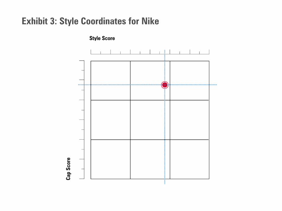
Exhibit 3: Style Coordinates for Nike

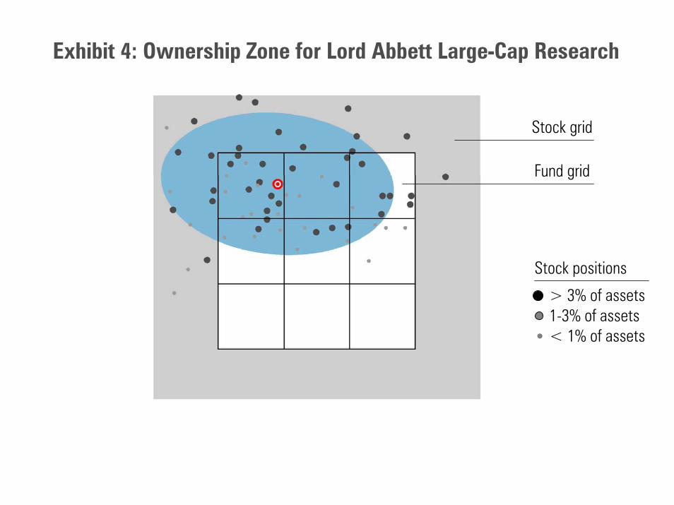
Exhibit 4: Ownership Zone for Lord Abbett Large-Cap Research

Stock grid

Fund grid

> 3% of assets1-3% of assets< 1% of assets.

Stock positions

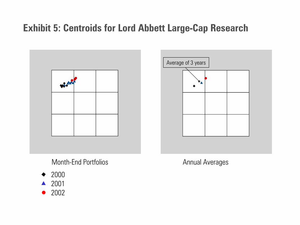
Exhibit 5: Centroids for Lord Abbett Large-Cap Research

200020012002

Month-End Portfolios Annual Averages

Average of 3 years

*

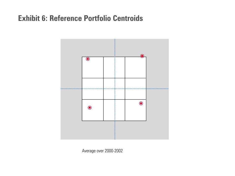
Exhibit 6: Reference Portfolio Centroids

Average over 2000-2002

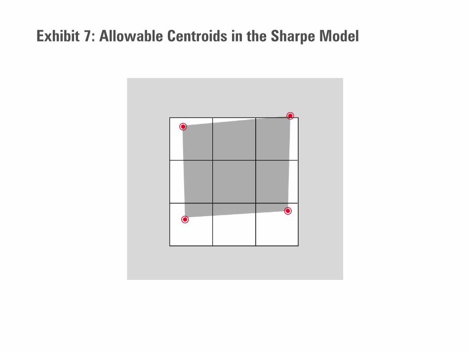
Exhibit 7: Allowable Centroids in the Sharpe Model

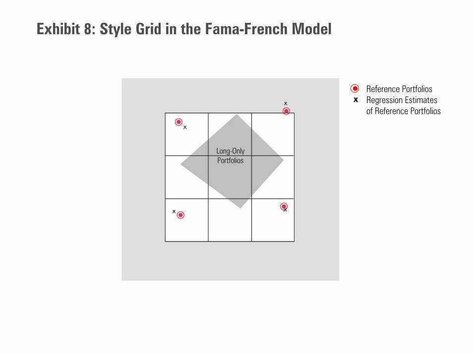
Exhibit 8: Style Grid in the Fama-French Model

Reference PortfoliosRegression Estimates of Reference Portfolios

Long Only Portfolios

x

Long-OnlyPortfolios

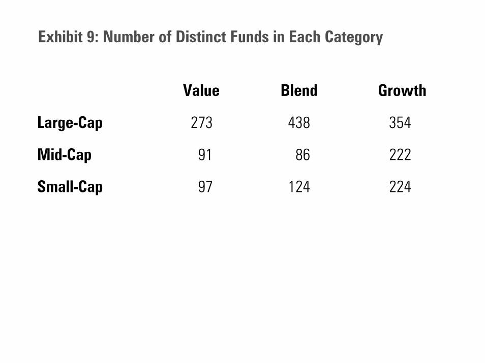
Exhibit 9: Number of Distinct Funds in Each Category

Value Blend Growth

Large-Cap 273 438 354

Mid-Cap 91 86 222

Small-Cap 97 124 224

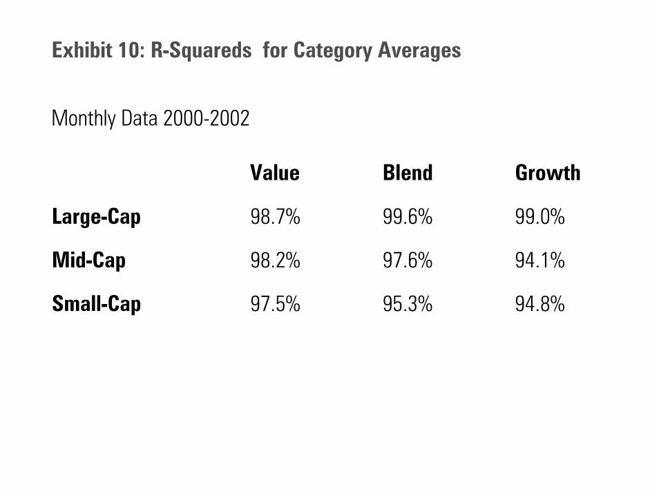
Exhibit 10: R-Squareds for Category Averages

Monthly Data 2000-2002

Value Blend Growth

Large-Cap 98.7% 99.6% 99.0%

Mid-Cap 98.2% 97.6% 94.1%

Small-Cap 97.5% 95.3% 94.8%

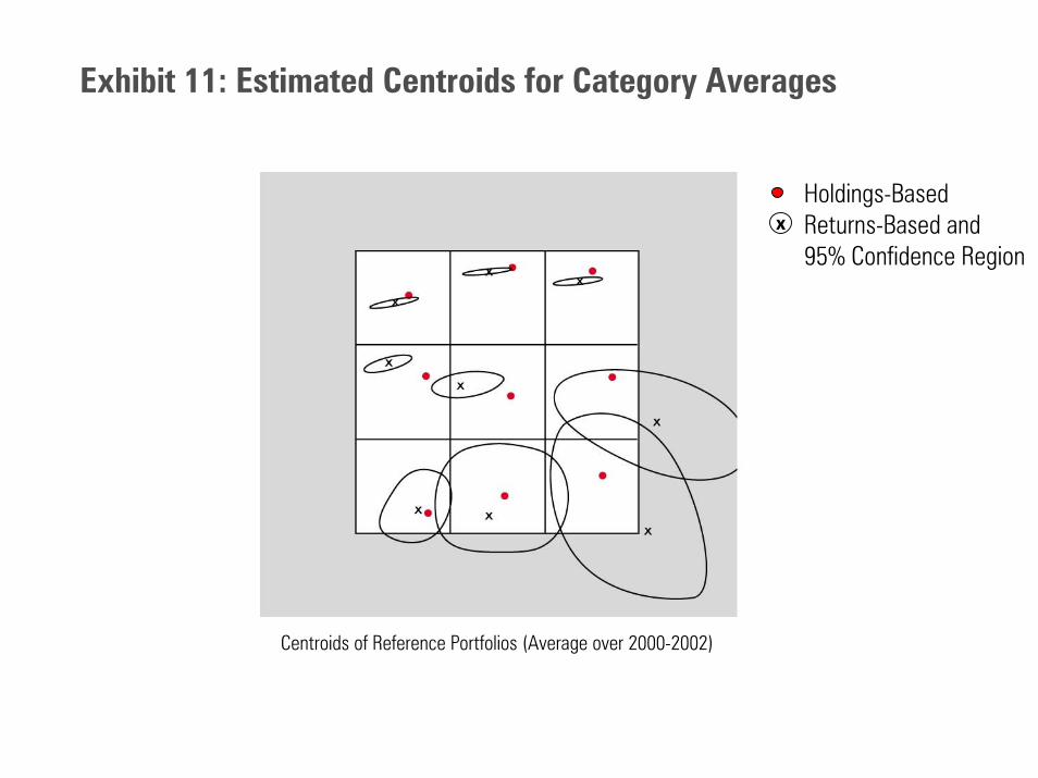
Exhibit 11: Estimated Centroids for Category Averages

Centroids of Reference Portfolios (Average over 2000-2002)

Holdings-BasedReturns-Based and 95% Confidence Region

x

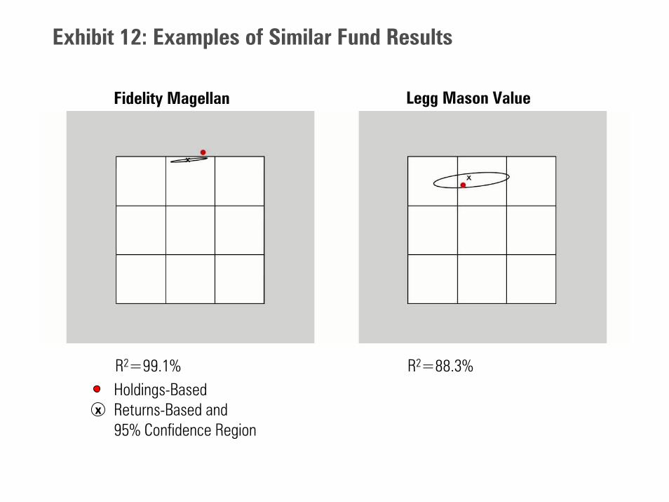
Exhibit 12: Examples of Similar Fund Results

Fidelity Magellan Legg Mason Value

R2=99.1% R2=88.3%Holdings-BasedReturns-Based and 95% Confidence Region

x

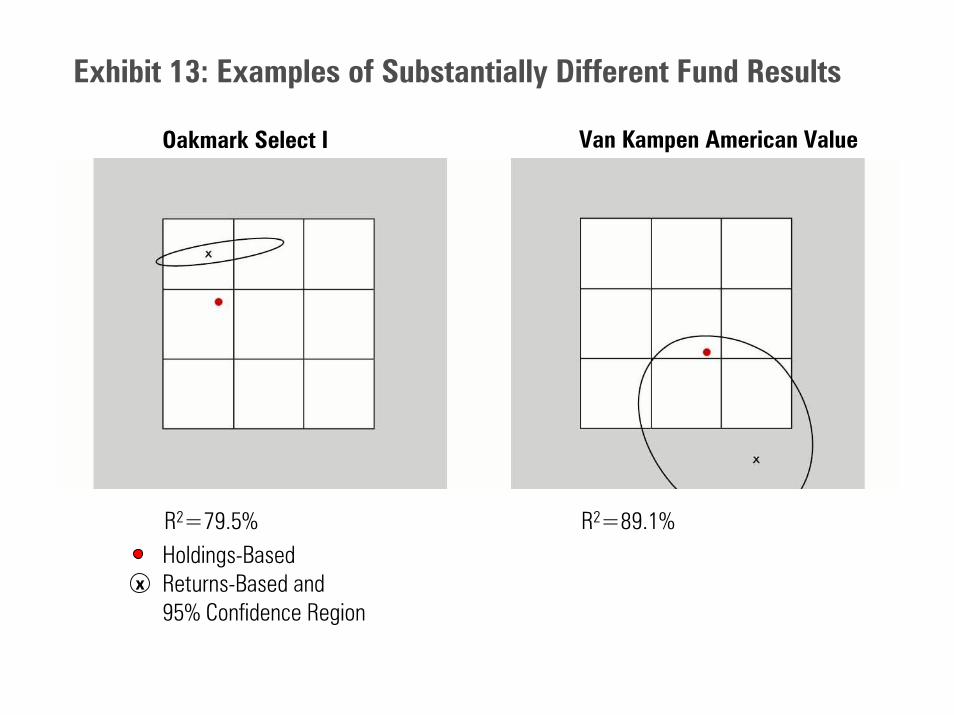
Exhibit 13: Examples of Substantially Different Fund Results

Oakmark Select I Van Kampen American Value

R2=79.5% R2=89.1%Holdings-BasedReturns-Based and 95% Confidence Region

x

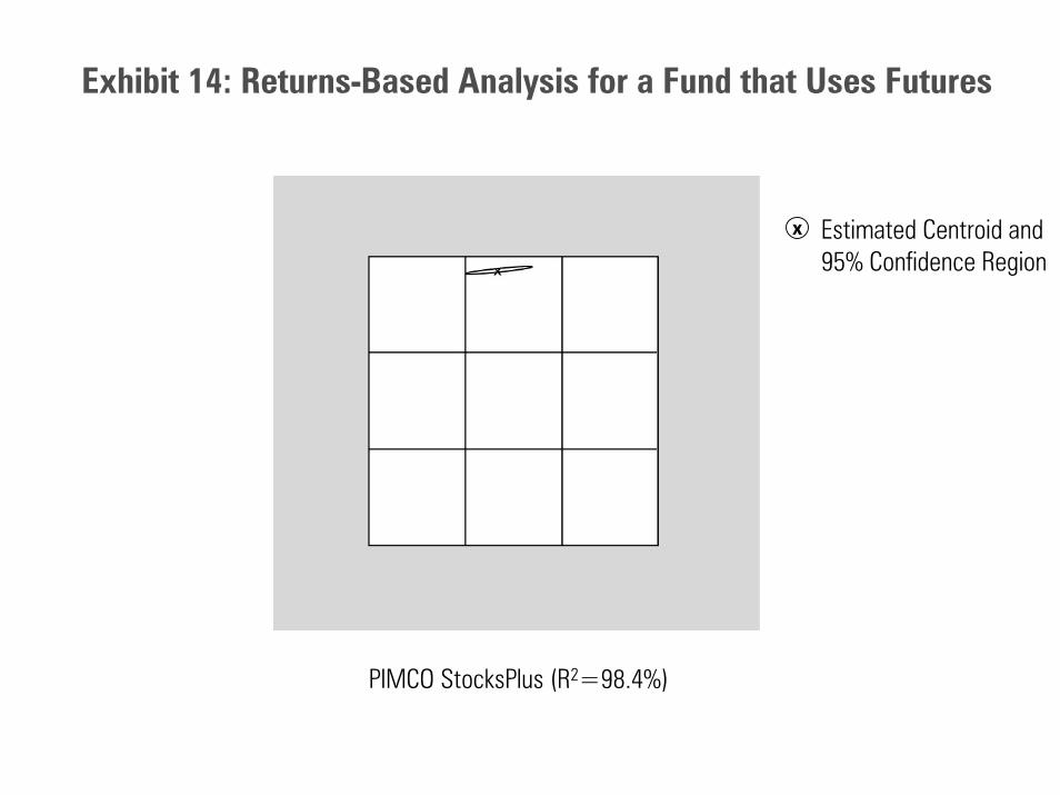
Exhibit 14: Returns-Based Analysis for a Fund that Uses Futures

PIMCO StocksPlus (R2=98.4%)

Estimated Centroid and 95% Confidence Region

x

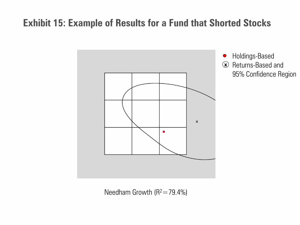
Exhibit 15: Example of Results for a Fund that Shorted Stocks

Needham Growth (R2=79.4%)

Holdings-BasedReturns-Based and 95% Confidence Region

x

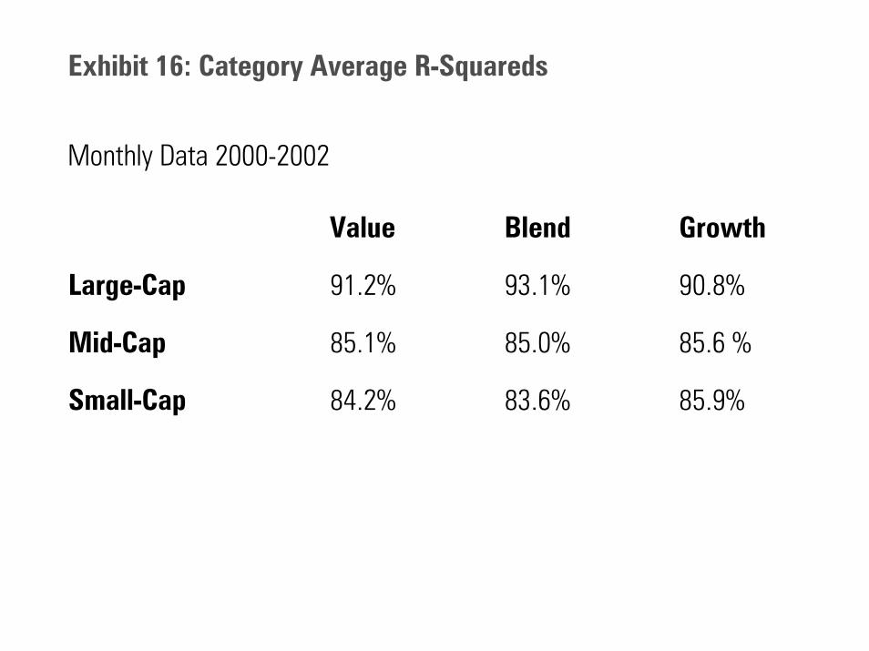
Exhibit 16: Category Average R-Squareds

Monthly Data 2000-2002

Value Blend Growth

Large-Cap 91.2% 93.1% 90.8%

Mid-Cap 85.1% 85.0% 85.6 %

Small-Cap 84.2% 83.6% 85.9%

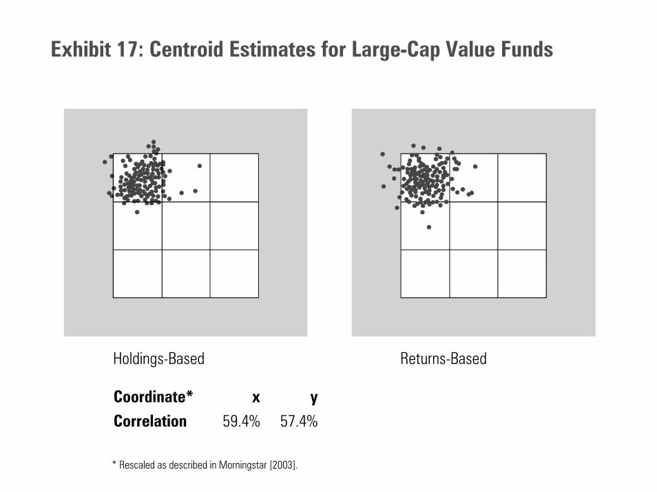
Exhibit 17: Centroid Estimates for Large-Cap Value Funds

57.4%59.4%CorrelationyxCoordinate*

Holdings-Based Returns-Based

* Rescaled as described in Morningstar [2003].

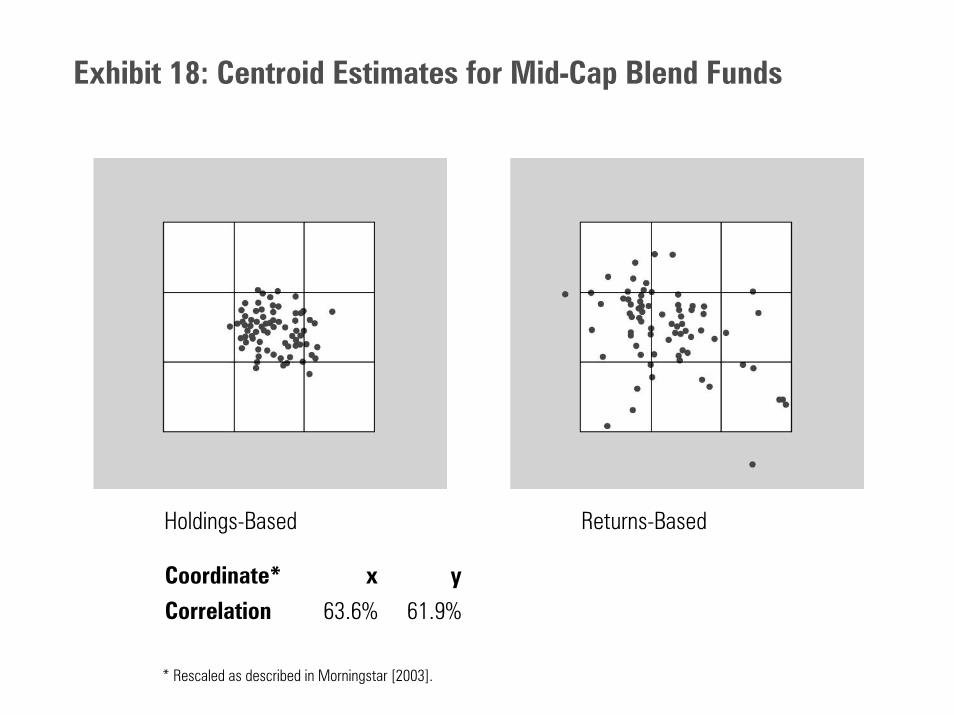
Exhibit 18: Centroid Estimates for Mid-Cap Blend Funds

61.9%63.6%CorrelationyxCoordinate*

Holdings-Based Returns-Based

* Rescaled as described in Morningstar [2003].

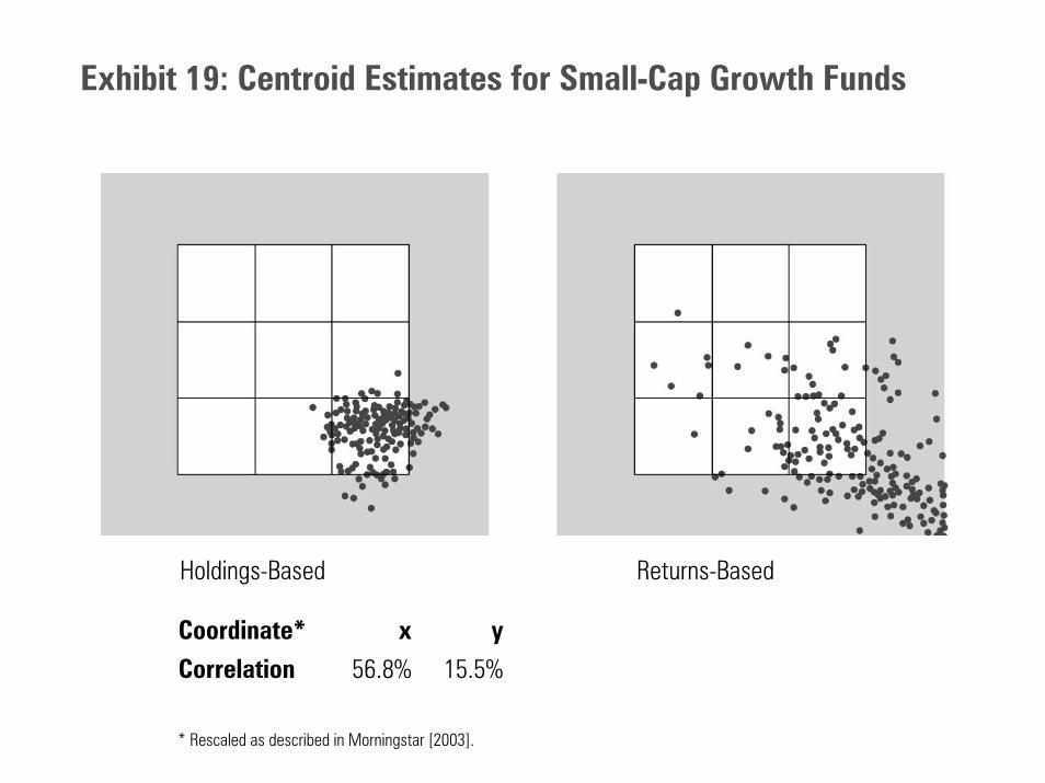
Exhibit 19: Centroid Estimates for Small-Cap Growth Funds

15.5%56.8%CorrelationyxCoordinate*

Holdings-Based Returns-Based

* Rescaled as described in Morningstar [2003].

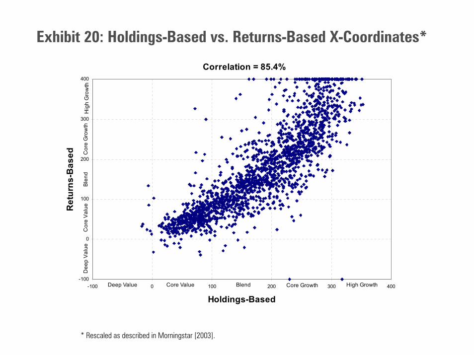
Exhibit 20: Holdings-Based vs. Returns-Based X-Coordinates*

Correlation = 85.4%

-100

0

100

200

300

400

-100 0 100 200 300 400

Holdings-Based

Ret

urns

-Bas

ed

Deep Value Core Value Blend Core Growth High Growth

Dee

p Va

lue

Cor

e Va

lue

Blen

dC

ore

Gro

wth

Hig

h G

row

th

* Rescaled as described in Morningstar [2003].

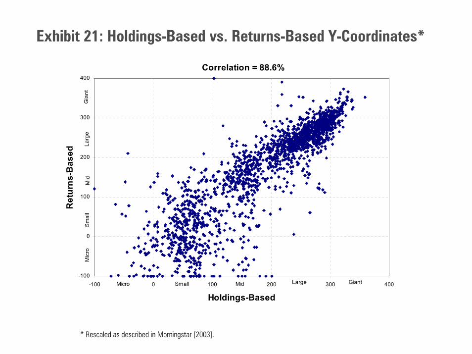
Exhibit 21: Holdings-Based vs. Returns-Based Y-Coordinates*

Correlation = 88.6%

-100

0

100

200

300

400

-100 0 100 200 300 400

Holdings-Based

Ret

urns

-Bas

ed

Micro Small Mid Large Giant

Mic

roSm

all

Mid

Larg

eG

iant

* Rescaled as described in Morningstar [2003].

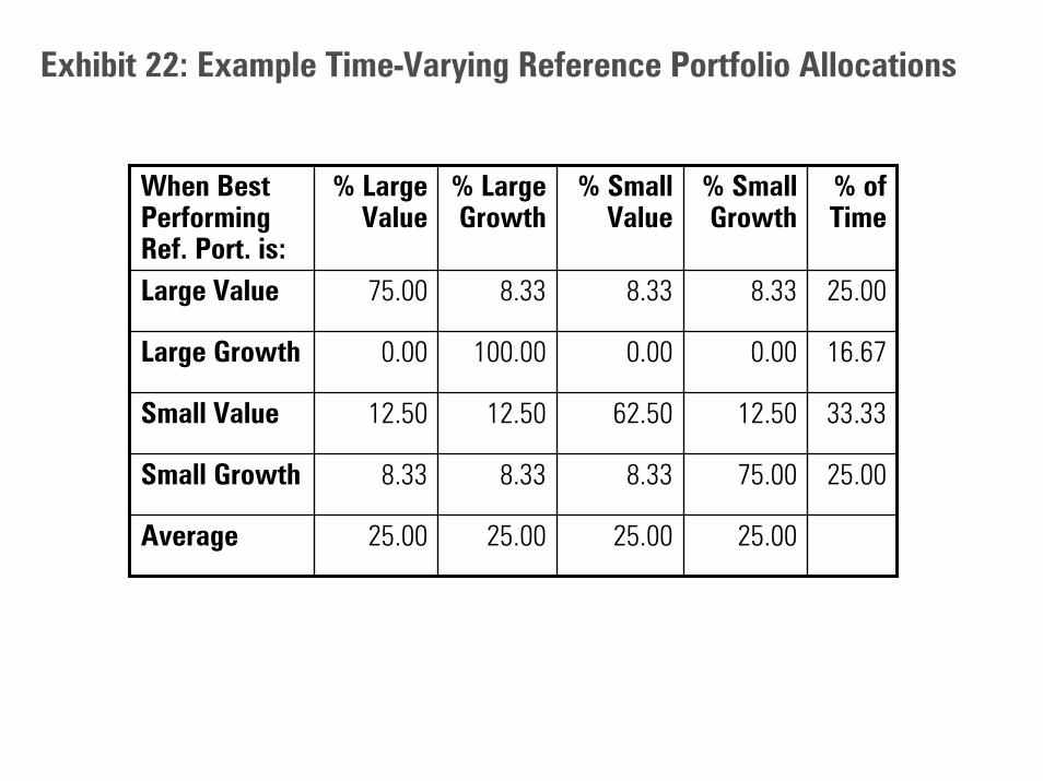
Exhibit 22: Example Time-Varying Reference Portfolio Allocations

25.0025.0025.0025.00Average

25.0075.008.338.338.33Small Growth

33.3312.5062.5012.5012.50Small Value

16.670.000.00100.000.00Large Growth

25.008.338.338.3375.00Large Value

% ofTime

% SmallGrowth

% SmallValue

% LargeGrowth

% LargeValue

When BestPerformingRef. Port. is:

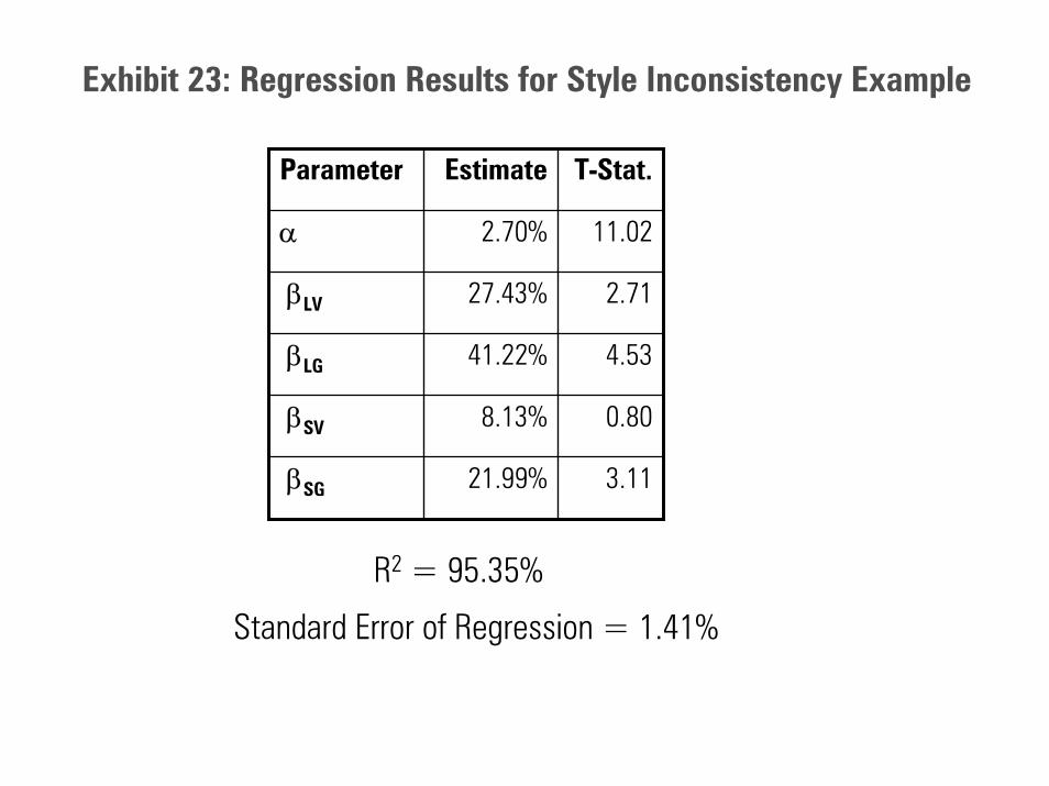
Exhibit 23: Regression Results for Style Inconsistency Example

3.1121.99% βSG

0.808.13% βSV

4.5341.22% βLG

2.7127.43% βLV

11.022.70%α

T-Stat.EstimateParameter

R2 = 95.35%

Standard Error of Regression = 1.41%