HOLDER REGULARITY FOR DEGENERATE PARABOLIC OBSTACLE¨

HOLDER REGULARITY FOR DEGENERATE PARABOLIC OBSTACLEPROBLEMS

VERENA BOGELEIN, TEEMU LUKKARI, AND CHRISTOPH SCHEVEN

ABSTRACT. We prove that weak solutions to the obstacle problem for the porous mediumequation are locally Holder continuous, provided that the obstacle is Holder continuous.

1. INTRODUCTION

The porous medium equation

∂tu−∆um = 0,

PME for short, is an important prototype of a nonlinear parabolic equation. The namestems from modeling the flow of a gas in a porous medium. We restrict our attention to theslow diffusion case when m > 1. In this case the equation is degenerate with respect to u,which means that the modulus of ellipticity vanishes when the solution is zero. This leadsto interesting phenomena, for instance the existence of moving boundaries. The PME andits various generalizations have been extensively studied, and we refer to the monographs[7, 9, 16, 17] for the basic theory and further references.

In the current paper we are interested in the obstacle problem for the PME. This problemcan be fomulated as a variational inequality: formally, a function u solves the obstacleproblem with obstacle ψ if u ≥ ψ and

(1.1)∫

ΩT

∂tu(vm − um) +∇um · ∇(vm − um) dx dt ≥ 0

for all comparison maps v such that v ≥ ψ. A rigorous interpretation of the time term inthis inequality requires some care as a solution might not have a time derivative in a suitablesense, see [1, 5] and Definition 2.1 below. The classical references for parabolic obstacleproblems are [1, 14, 15], and some of the more recent ones are [4, 5, 6, 12, 13]. However,most of them are dealing with the obstacle problem for the parabolic p-Laplacian equation.An alternative to the variational inequality is to define the solution to the obstacle problemto be the smallest supersolution lying above the obstacle, see [2, 13] and Remark 2.3 below.We will not pursue the latter approach here.

The existence of appropriately defined weak solutions to the obstacle problem for thePME was shown in our previous paper [5]. These solutions belong to the class

Kψ(ΩT ) :=v ∈ C0

([0, T ];Lm+1(Ω)

): vm ∈ L2

(0, T ;H1(Ω)

), v ≥ ψ a.e. on ΩT

,

where ψ is a nonnegative obstacle function defined on a space-time cylinder ΩT = Ω ×(0, T ), Ω is a bounded domain in Rn, and T > 0. Here our aim is to complement theresults of [5] by establishing regularity for the solutions. The general guideline is thata solution to the obstacle problem should be as regular as a weak solution, as long asthe regularity of the obstacle allows it. Hence a solution to the obstacle problem shouldbe Holder continuous if the obstacle is, since a weak solution to the PME is in generalno better than Holder continuous. This can be seen from explicit examples, such as the

Date: September 23, 2015.2010 Mathematics Subject Classification. 35K65, 35B65, 35K86, 47J20.Key words and phrases. obstacle problem, porous medium equation, regularity.

1

2 V. BOGELEIN, T. LUKKARI, AND C. SCHEVEN

Barenblatt solution. In this respect, the following regularity result, which is the main resultof this paper, is optimal.

Theorem 1.1. Suppose that the obstacle ψ is Holder continuous in ΩT , and let u ∈Kψ(ΩT ) be a local weak solution to the obstacle problem for the PME in the sense ofDefinition 2.1. Then u is locally Holder continuous in ΩT .

The proof of the Holder continuity is based on two main elements: energy estimatesfor truncations, and a De Giorgi type iteration argument to extract pointwise informationfrom the energy estimates. The derivation of the energy estimates is intricate due to thenecessarily complicated definition of weak solutions to the obstacle problem. For instance,the solution itself is not usually admissible as a comparison map in the variational inequal-ity. In the iteration arguments, we need to construct cylinders with a proper scaling tobalance the different powers in the energy estimates. The scaling is intrinsic, as it dependson the solution itself. This method has been introduced in [10] for the analysis of degen-erate parabolic equations, cf. also [8, 9, 3]. More precisely, in order to compensate for theinhomogeneous scaling of the underlying equation, we work with cylinders of the type

Q%,θ%2(xo, to) = B%(xo)× (to − θ%2, to),

where the parameter θ is comparable to u1−m. Additional care is needed in dealing withthe degeneration of the porous medium equation, which occurs if the solution takes valuesclose to zero in the sense that its infimum is considerably smaller than its supremum.This case, which we call the degenerate regime, requires a different treatment than thenondegenerate regime, in which the equation heuristically behaves like a linear equationwith irregular coefficients. The proof is structured in such a way that both regimes aretreated in a unified way whenever it is possible in order to work out the similarities and thedifferences of the two regimes.

The regularity of the obstacle enters the argument via a restriction on the truncation lev-els, which is needed to ensure that the test functions do not violate the obstacle condition.

The paper is organized as follows. In §2, we give the exact definition of a weak solutionto the obstacle problem. In §3 we recall several technical results needed for the proofs. Weprove the energy estimates for truncations in §4. These estimates are then used in §5 toprove local boundedness of solutions, and finally in §6 to prove the Holder continuity.

2. THE OBSTACLE PROBLEM

In this section, we give the rigorous definition of a solution to the obstacle problem.For a bounded domain Ω ⊂ Rn in dimension n ∈ N≥2 and a time T > 0, we writeΩT := Ω× (0, T ) for the space-time cylinder. We consider continuous obstacle functionsψ ∈ C0(ΩT ,R≥0). For fixed m > 1, we recall that the solution space is defined by

Kψ(ΩT ) :=v ∈ C0

([0, T ];Lm+1(Ω)

): vm ∈ L2

(0, T ;H1(Ω)

), v ≥ ψ a.e. on ΩT

.

Furthermore, the class of admissible comparison functions is

K ′ψ(ΩT ) :=v ∈ Kψ(ΩT ) : ∂t(v

m) ∈ Lm+1m (ΩT )

.

Since the time derivative of a solution u ∈ Kψ(ΩT ) to the obstacle problem might not existin a sufficiently strong sense, we have to introduce a weak formulation of the time term inthe variational inequality (1.1). To this end, we follow the approach by Alt & Luckhaus [1]and define for every u ∈ Kψ(ΩT ) and every comparison map v ∈ K ′ψ(ΩT )

(2.1) 〈〈∂tu, αη(vm − um)〉〉 :=

∫ΩT

η[α′[

1m+1u

m+1 − uvm]− αu∂tvm

]dz,

where α ∈ W 1,∞0 ([0, T ],R≥0) and η ∈ C1

0 (Ω,R≥0) denote cut-off functions in time,respectively in space.

HOLDER REGULARITY FOR DEGENERATE PARABOLIC OBSTACLE PROBLEMS 3

We are now in a position to define the notion of a local weak solution to the obstacleproblem.

Definition 2.1. A nonnegative function u ∈ Kψ(ΩT ) is a local weak solution to the ob-stacle problem for the porous medium equation if and only if

(2.2) 〈〈∂tu, αη(vm − um)〉〉+

∫ΩT

α∇um · ∇(η(vm − um)

)dz ≥ 0

holds true for all comparison maps v ∈ K ′ψ(ΩT ), every cut-off function in time α ∈W 1,∞

0 ([0, T ],R≥0) and every cut-off function in space η ∈ C10 (Ω,R≥0).

Remark 2.2. Since u ∈ C0([0, T ];Lm+1(Ω)), this definition is consistent with the notionof weak solution used in [5, Def. 2.1]. This means that for more general cut-off functionsin time with α(0) 6= 0, the above notion of solution implies

〈〈∂tu, αη(vm − um)〉〉uo +

∫ΩT


)dz ≥ 0

for uo := u(·, 0) if we define

〈〈∂tu, αη(vm − um)〉〉uo :=

∫ΩT

η[α′[

1m+1u

m+1 − uvm]− αu∂tvm

]dz

+ α(0)

∫Ω

η[

1m+1u

m+1o − uovm(·, 0)

]dx.

For obstacles ψ with

ψm ∈ L2(0, T ;H1(Ω)

), ∂t(ψ

m) ∈ Lm+1m (ΩT ) and ψm(·, 0) ∈ H1(Ω),

an existence result for local weak solutions is contained in our earlier work [5].Moreover, from [5, Lemma 3.2] we know that a local weak solution with ∂tu ∈

L2(0, T ;H−1(Ω)) is also a local strong solution in the sense that for all comparison mapsv ∈ Kψ(ΩT ), every cut-off function in time α ∈ W 1,∞([0, T ],R≥0) with α(T ) = 0 andevery cut-off function in space η ∈ C1

0 (Ω,R≥0) we have∫ T

0

〈∂tu, αη(vm − um)〉dt+

∫ΩT


)dz ≥ 0,

where here, 〈·, ·〉 denotes the dual pairing between H−1(Ω) and H10 (Ω).

Remark 2.3. An alternative to the variational inequality desribed above is to define thesolution to the obstacle problem to be the smallest weak supersolution lying above theobstacle ψ. This approach is used in [13] in a nonlinear parabolic setting, and in [2] for thePME. It is analogous to the balayage concept of classical potential theory.

Existence and uniqueness of the smallest supersolution follow quite easily from the def-initions. However, the connection between the smallest supersolution and the variationalsolutions studied here is less clear. In this direction, we have an approximation propertyfor the smallest supersolution: for continuous compactly supported obstacles, the small-est supersolution is a pointwise limit of variational solutions. See [2] for the proof. Theapproximation property together with a stability result from [5] implies that the smallestsupersolution is also a variational solution for sufficiently smooth obstacles. Further, sinceour Holder estimate depends on the obstacle only via its Holder norm, Theorem 1.1 holdsalso for the smallest supersolution.

The question whether all variational solutions are also smallest supersolutions remainsa very interesting open problem.


3. PRELIMINARIES

3.1. Notation. We use the notation Q%,θ(zo) := B%(xo)× (to − θ, to) ⊂ Rn+1 for back-ward parabolic cylinders, where the point zo = (xo, to) ∈ Rn+1 is the vertex of thecylinder, and %, θ > 0.

3.2. Auxiliary material. For later reference, we recall the parabolic version of theGagliardo-Nirenberg inequality.

Lemma 3.1. Let Q%,θ(zo) ⊂ Rn+1 be a parabolic cylinder and 1 < p, r <∞. For every

u ∈ L∞(to − θ, to;Lr(B%(xo)) ∩ Lp(to − θ, to;W 1,p(B%(xo))

we have u ∈ Lq(Q%,θ(zo)) for q = p(1 + rn ) with the estimate∫

Q%,θ(zo)

|u|q dz ≤ c(

supt∈(to−θ,to)

∫B%(xo)×t

|u|r dx

) pn∫Q%,θ(zo)

(|∇u|p +

∣∣∣u%

∣∣∣p)dz,

where c = c(n, p, r).

The proof of the following well-known lemma can be found e.g. in [11, Lemma 7.1].

Lemma 3.2. Let (Xi)i∈N0 be a sequence of positive real numbers with

Xi+1 ≤ CBiX1+αi for all i ∈ N0,

for constants C,α > 0 and B > 1. Then

X0 ≤ C−1αB−

1α2

implies Xi → 0 as i→∞.

We will also use DeGiorgi’s isoperimetric inequality. See e.g. [9, §2, Lemma 2.2] forthe proof.

Lemma 3.3. Let v ∈ W 1,1(B%(xo)), and let k < ` be real numbers. There exists aconstant c = c(n), such that

(`− k)|B%(xo) ∩ v > `| ≤ c %n+1

|B%(xo) ∩ v < k|

∫B%(xo)∩k<v<`

|∇v|dx.

3.3. Mollification in time. In order to deal with the possible lack of differentiability intime of weak solutions, the following time mollification of functions v : ΩT → R hasproved to be useful.

(3.1) [[v]]h(x, t) :=1

h

∫ t

0

es−th v(x, s) ds.

In the following lemma, we list some elementary properties of this mollification that willbe needed in the proof later (cf. [15]).

Lemma 3.4. Let p ≥ 1.

(i) If v ∈ Lp(ΩT ) then [[v]]h → v in Lp(ΩT ) as h ↓ 0 and

∂t[[v]]h = 1h (v − [[v]]h) ∈ Lp(ΩT ) for every h > 0.

(ii) If ∇v ∈ Lp(ΩT ,Rn) then ∇[[v]]h = [[∇v]]h and ∇[[v]]h → ∇v in Lp(ΩT ,Rn) ash ↓ 0.

(iii) If v ∈ C0(ΩT ), then [[v]]h → v uniformly in ΩT as h ↓ 0.


4. ENERGY ESTIMATES

4.1. Caccioppoli type estimates. Here, we derive energy estimates for the truncated func-tions

[um − km]+ := maxum − km, 0 and [um − km]− := maxkm − um, 0,where k > 0 denotes a constant.

Lemma 4.1. Let Q1 := Q%1,θ1(zo) b ΩT and Q2 := Q%2,θ2(zo) ⊂ Q1 be two cylinderswith %2 < %1, θ2 < θ1, and assume that ψ ∈ C0(ΩT ,R≥0). Then, for every local weaksolution u ∈ Kψ(ΩT ) to the obstacle problem for the porous medium equation in the senseof Definition 2.1, we have the following estimates.

(i) For every k ≥ supQ1ψ we have

supt∈(to−θ2,to)

∫B%2 (xo)×t

u1−m[um − km]2+ dx+

∫Q2

∣∣∇[um − km]+∣∣2 dz

≤ c(m)

(1

(%1 − %2)2+

k1−m

θ1 − θ2

)∫Q1

[um − km]2+ dz.

(ii) For every k > 0, we have

supt∈(to−θ2,to)

k1−m∫B%2 (xo)×t

[um − km]2− dx+

∫Q2

∣∣∇[um − km]−∣∣2 dz

≤ c(m)

(%1 − %2)2

∫Q1

[um − km]2− dz +c(m)

θ1 − θ2

∫Q1

∫ [um−km]−

0

(km − τ)1−mm τ dτ dz.

Proof of (i). By restricting ourselves to a compact subdomain of ΩT if necessary, wemay assume ψ ∈ C0(ΩT ), so that Lemma 3.4 (iii) is applicable to v = ψ. More-over, we assume zo = 0 for notational convenience. We choose a cut-off functionα ∈ W 1,∞

0 ([−θ1, 0],R≥0) and η ∈ C10 (B%1 ,R≥0). In the variational inequality (2.2),

we choosevmh := [[um]]h − [[um − km]]h,+ + ‖ψm − [[ψm]]h‖L∞(ΩT )

as comparison map for u, for some h > 0. Here, we employed the short-hand notation[[um − km]]h,+ := [ [[um − km]]h ]+ = [[[um]]h − km]+ with the mollification [[·]]h asdefined in (3.1). This map satisfies

∂tvmh = ∂t min[[um]]h, k

m ∈ Lm+1m (ΩT ).

The comparison map vh is admissible because we have

vmh = min[[um]]h, km+ ‖ψm − [[ψm]]h‖L∞(ΩT ) ≥ ψm on Q1,

since u ≥ ψ a.e. on ΩT and k ≥ supQ1ψ by assumption. We note that it is sufficient to

check the obstacle condition for vh on supp(αη) ⊂ Q1. We therefore know

(4.1) Ih + IIh := 〈〈∂tu, αη2(vmh − um)〉〉+

∫Q1

α∇um · ∇(η2(vmh − um)

)dz ≥ 0.

For the estimate of Ih, we use Lemma 3.4 (i) to calculate∫Q1

η2αu∂tvmh dz

=

∫Q1

η2α[[um]]1m

h ∂tvmh dz +

∫Q1∩[[um]]h≤km

η2α(u− [[um]]

1m

h

)1h (um − [[um]]h

)dz

≥∫Q1

η2α[[um]]1m

h ∂t([[um]]h − [[um − km]]h,+

)dz

=

∫Q1

η2(α mm+1∂t[[u

m]]m+1m

h + α′[[um]]1m

h [[um − km]]h,+)

dz


+

∫Q1

η2α∂t[[um]]

1m

h [[um − km]]h,+ dz.

The last integrand can be re-written using the identity

(4.2) ∂t[[um]]

1m

h [[um − km]]h,+ =1

m

∂

∂t

∫ [[um−km]]h,+

0

(km + τ)1−mm τ dτ.

Plugging this into the preceding inequality and integrating by parts, we deduce∫Q1

η2αu∂tvmh dz ≥

∫Q1

η2α′(− m

m+1 [[um]]m+1m

h + [[um]]1m

h [[um − km]]h,+)

dz

− 1m

∫Q1

η2α′∫ [[um−km]]h,+

0

(km + τ)1−mm τ dτ dz.

Recalling definition (2.1) we deduce

Ih =

∫Q1

η2[α′[

1m+1u

m+1 − uvmh]− αu∂tvmh

]dz

≤∫Q1

η2α′(

1m+1u

m+1 − u([[um]]h − [[um − km]]h,+ + ‖ψm − [[ψm]]h‖L∞

)dz

+

∫Q1

η2α′ mm+1 [[um]]

m+1m

h − [[um]]1m

h [[um − km]]h,+)

dz

+ 1m

∫Q1

η2α′∫ [[um−km]]h,+

0


Lemma 3.4 implies [[um]]h → um in Lm+1m (Q1) as well as ‖ψm − [[ψm]]h‖L∞ → 0 as

h ↓ 0. As a consequence, the sum of the first two integrals on the right-hand side vanishesin the limit h ↓ 0 and we infer

(4.3) lim suph↓0

Ih ≤ 1m

∫Q1

η2α′∫ [um−km]+

0


Next, we note that ∇(η2(vmh − um)) → −∇(η2[um − km]+) in L2(Q1) as h ↓ 0 byLemma 3.4. Using moreover the identity

(4.4) ∇um = ∇[um − km]+ a.e. on ΩT ∩ u ≥ k,we calculate

limh↓0

IIh = −∫Q1

α∇um · ∇(η2[um − km]+

)dz(4.5)

= −∫Q1

αη2∣∣∇[um − km]+

∣∣2 dz

− 2

∫Q1

αη∇[um − km]+ · ∇η[um − km]+ dz

≤ − 12

∫Q1

αη2∣∣∇[um − km]+

∣∣2 dz + 2

∫Q1

α|∇η|2[um − km]2+ dz.

Combining (4.3) and (4.5) with (4.1), we arrive at

12

∫Q1

αη2∣∣∇[um − km]+

∣∣2 dz

≤ 1m

∫Q1

η2α′∫ [um−km]+

0

(km + τ)1−mm τ dτ dz + 2

∫Q1

α|∇η|2[um − km]2+ dz.

Now, we choose η ∈ C10 (B%1

,R≥0) with η ≡ 1 on B%2and |∇η| ≤ 2

%1−%2. Moreover,

for any time t ∈ (−θ2, 0) and ε > 0, we choose α ∈ W 1,∞0 (−θ1, 0) with α(s) = θ1+s

θ1−θ2


for s ∈ (−θ1,−θ2), α ≡ 1 on (−θ2, t − ε), α(s) = t−sε for s ∈ (t − ε, t) and α ≡ 0 on

(t, 0). Using the preceding estimate with this choice of cut-off functions and letting ε ↓ 0,we infer

1m

∫B%2×t

∫ [um−km]+

0

(km + τ)1−mm τ dτ dx+ 1

2

∫Q2

∣∣∇[um − km]+∣∣2 dz(4.6)

≤ 8

(%1 − %2)2

∫Q1

[um − km]2+ dz

+1

m(θ1 − θ2)

∫Q1

∫ [um−km]+

0


This implies the claimed energy estimate by bounding the left-hand side from below viathe inequality

1m

∫ [um−km]+

0

(km + τ)1−mm τ dτ ≥ 1

mu1−m

∫ [um−km]+

0

τ dτ = 12mu

1−m[um − km]2+

and the right-hand side via

1m

∫ [um−km]+

0

(km + τ)1−mm τ dτ ≤ k1−m

m

∫ [um−km]+

0

τ dτ = k1−m

2m [um − km]2+.

Proof of (ii). Here, we consider an arbitrary k > 0. Since most of the proof of (ii) isanalogous to that of (i), we only indicate the necessary changes. As comparison maps, wenow choose

vmh := [[um]]h + [[um − km]]h,− + ‖ψm − [[ψm]]h‖L∞(Q1),

which satisfy

∂tvmh = ∂t max[[um]]h, k

m ∈ Lm+1m (ΩT ).

These maps are admissible since vmh ≥ [[um]]h + ‖ψm − [[ψm]]h‖L∞(Q1) ≥ ψm holds onΩT . Now we can repeat the calculations leading to (4.6), but now replacing [[um−km]]h,+by −[[um − km]]h,− . Instead of the identity (4.2), we now use

∂t[[um]]

1m

h (−[[um − km]]h,−) =1

m

∂

∂t

∫ [[um−km]]h,−

0

(km − τ)1−mm τ dτ.

Moreover, we replace (4.4) by∇um = −∇[um− km]− on ΩT ∩u ≤ k. The remainderof the proof works as in the case of (i), and analogously to (4.6), we derive the estimate

1m

∫B%2×t

∫ [um−km]−

0

(km − τ)1−mm τ dτ dx+ 1

2

∫Q2

∣∣∇[um − km]−∣∣2 dz

≤ 8

(%1 − %2)2

∫Q1

[um − km]2− dz

+1

m(θ1 − θ2)

∫Q1

∫ [um−km]−

0

(km − τ)1−mm τ dτ dz

for every t ∈ (−θ2, 0). This implies the claim by estimating the left-hand side from belowby

1m

∫ [um−km]−

0

(km−τ)1−mm τ dτ ≥ k1−m

m

∫ [um−km]−

0

τ dτ = 12mk

1−m[um−km]2− .


4.2. The logarithmic estimate. In this section we derive an estimate that will be usefullater to compare the measures of certain super-level sets on different time slices. To thisend, for parameters 0 < γ < Γ, we consider the function

(4.7) φ(v) := φΓ,γ(v) :=

[log( Γ

Γ + γ − v

)]+

for v < Γ + γ.

We note that φ(v) = 0 for v ≤ γ, and for v ≤ Γ we have the estimates

(4.8) 0 ≤ φ(v) ≤ log(

Γγ

)and 0 ≤ φ′(v) ≤ 1

γ for v 6= γ.

Moreover, the function satisfies the differential equation φ′′ = (φ′)2 for v 6= γ. We pointout that contrary to φ, the squared function φ2 is differentiable on [0,Γ] with

(4.9) (φ2)′ = 2φφ′ on [0,Γ] and (φ2)′′ = 2(1 + φ)(φ′)2 on [0,Γ] \ γ.In particular (φ2)′ is Lipschitz, which will be crucial in the proof below.

Lemma 4.2. We consider two concentric balls B%2(xo) b B%1(xo) b Ω and times 0 <t1 < t2 < T and abbreviate Q1 := B%1

(xo) × (t1, t2). Let u ∈ Kψ(ΩT ) be a localweak solution to the obstacle problem for the porous medium equation in the sense ofDefinition 2.1, for an obstacle ψ ∈ C0(ΩT ,R≥0). For some k > 0 with k ≥ supQ1

ψ wedefine Γ := supQ1

[um − km]+ and denote by φ = φΓ,γ the function introduced in (4.7)for some parameter γ ∈ (0,Γ). Then we have

supt∈(t1,t2)

∫B%2 (xo)×t

u1−mφ2([um − km]+

)dx

≤ k1−m∫B%1 (xo)×t1

φ2([um − km]+

)dx

+8m

(%1 − %2)2

∫B%1 (xo)×(t1,t2)

φ([um − km]+

)dz.

Proof. Since the asserted estimate is of local nature, we may assume ψ ∈ C0(ΩT ). Be-cause both sides of the asserted estimate are continuous in k, it suffices to prove the claimfor every k > supQ1

ψ. For the sake of convenience, we moreover assume xo = 0. In thevariational inequality (2.2) we consider cut-off functions α ∈ W 1,∞

0 ((t1, t2),R≥0) andη ∈ C1

0 (B%1,R≥0). For a suitable λ > 0, we wish to choose

vmh := [[um]]h − λ(φ2)′([[um − km]]h,+) + ‖ψm − [[ψm]]h‖L∞

as comparison map in (2.2). Since (φ2)′ is a Lipschitz map, the chain rule implies ∂tvmh ∈Lm+1m (ΩT ) and ∇vmh ∈ L2(ΩT ). Moreover, vh satisfies the obstacle constraint for a

sufficiently small choice of λ > 0 since for [[um]]h ≤ km we have

vmh = [[um]]h + ‖ψm − [[ψm]]h‖L∞ ≥ ψm

by the obstacle condition for um, while for [[um]]h > km we have

vmh > km − λ(φ2)′([[um − km]]h,+) ≥ supQ1

ψm,

if we choose λ ≤ (km−supQ1ψm)

sup[0,Γ](φ2)′ . This means that vmh ≥ ψm holds on Q1 ⊃ supp(αη),

which makes vh admissible in (2.2). We thereby get

(4.10) Ih + IIh := 〈〈∂tu, αη2(vmh − um)〉〉+

∫ΩT

α∇um · ∇(η2(vmh − um)

)dz ≥ 0.

For the analysis of Ih, we first use Lemma 3.4 (i) to compute

∂tvmh = ∂t[[u

m]]h − λ(φ2)′′([[um − km]]h,+)∂t[[um]]h

= 1h

(um − [[um]]h

)(1− λ(φ2)′′([[um − km]]h,+)

).


We note that the terms involving (φ2)′′ are a.e. well-defined since ∂t[[um]]h vanishes a.e.on the set [[um]]h = km + γ. By diminishing the value of λ > 0 once more we canachieve λ ≤ [sup[0,Γ](φ

2)′′]−1 and estimate(u− [[um]]

1m

h

)∂tv

mh ≥

(u− [[um]]

1m

h

)1h

(um − [[um]]h

)(1− λ sup(φ2)′′

)≥ 0.

This implies∫ΩT

αη2u∂tvmh dz ≥

∫ΩT

αη2[[um]]1m

h ∂tvmh dz

=

∫ΩT

αη2[[um]]1m

h ∂t

([[um]]h − λ(φ2)′([[um − km]]h,+)

)dz

=

∫ΩT

η2(α mm+1∂t[[u

m]]m+1m

h + λα′[[um]]1m

h (φ2)′([[um − km]]h,+))

dz

+ λ

∫ΩT

αη2∂t[[um]]

1m

h (φ2)′([[um − km]]h,+) dz.

We re-write the last integrand using the equation

∂t[[um]]

1m

h (φ2)′([[um − km]]h,+) =1

m

∂

∂t

∫ [[um−km]]h,+

0

(km + τ)1−mm (φ2)′(τ) dτ.

Combining the two preceding formulae and integrating by parts we deduce∫ΩT

αη2u∂tvmh dz ≥

∫ΩT

η2α′(− m

m+1 [[um]]m+1m

h + λ[[um]]1m

h (φ2)′([[um − km]]h,+))

dz

− λm

∫ΩT

α′η2

∫ [[um−km]]h,+

0

(km + τ)1−mm (φ2)′(τ) dτ dz.

Now we recall the definition (2.1) to conclude

Ih =

∫ΩT

η2[α′[

1m+1u

m+1 − uvmh]− αu∂tvmh

]dz

≤∫

ΩT

η2α′[

1m+1u

m+1 − u([[um]]h − λ(φ2)′([[um − km]]h,+) + ‖ψm − [[ψm]]h‖L∞

)]dz

−∫

ΩT

η2α′(− m

m+1 [[um]]m+1m

h + λ[[um]]1m

h (φ2)′([[um − km]]h,+))

dz

+ λm

∫ΩT

α′η2

∫ [[um−km]]h,+

0

(km + τ)1−mm (φ2)′(τ) dτ dz.

Because [[um]]h → um in Lm+1m (Q1) and ‖ψm− [[ψm]]h‖L∞ → 0 as h ↓ 0 by Lemma 3.4,

the first two integrals on the right-hand side cancel each other in the limit h ↓ 0. Lettingh ↓ 0 therefore yields

(4.11) lim suph↓0

Ih ≤ λm

∫ΩT

α′η2

∫ [um−km]+

0

(km + τ)1−mm (φ2)′(τ) dτ dz.

Now, we turn our attention to the term IIh. We claim that

η2(vmh − um) −λη2(φ2)′([um − km]+) weakly in L2(t1, t2;H1(B%1)),

as h ↓ 0. First we note that this convergence holds strongly in L2(Q1) byLemma 3.4 (i) and (iii). Furthermore, the sequence on the left-hand side is bounded inL2(t1, t2;H1(B%1

)) by Lemma 3.4 (ii) and because (φ2)′ is Lipschitz. This implies theclaimed weak convergence, which in turn implies

limh↓0

IIh = −λ∫

ΩT

α∇um · ∇[η2(φ2)′([um − km]+)

]dz


= −λ∫

ΩT

αη2|∇um|2(φ2)′′([um − km]+) dz

+ 2

∫ΩT

αη∇um · ∇η(φ2)′([um − km]+) dz.

The last integral is well-defined since∇um = 0 a.e. on the set um = km + γ. Next, weapply Young’s inequality in the last integral and infer

limh↓0

IIh ≤ λ∫

ΩT

αη2|∇um|2[2φ(φ′)2 − (φ2)′′

]([um − km]+) dz(4.12)

+ 2λ

∫ΩT

α|∇η|2φ([um − km]+) dz

≤ 2λ

∫ΩT

α|∇η|2φ([um − km]+) dz.

The last estimate is a consequence of (4.9), which implies 2φ(φ′)2−(φ2)′′ = −2(φ′)2 ≤ 0.Next, we plug (4.11) and (4.12) into (4.10) and divide by λ. This provides us with theestimate

1m

∫ΩT

α′η2

∫ [um−km]+

0

(km + τ)1−mm (φ2)′(τ) dτ dz

+ 2

∫ΩT

α|∇η|2φ([um − km]+) dz ≥ 0.

Now we choose η ∈ C10 (B%1

,R≥0) as a standard cut-off function with η ≡ 1 on B%2and

|∇η| ≤ 2%1−%2

onB%1 . For the choice of α, we fix t ∈ (t1, t2) and some 0 < ε < 12 (t−t1).

Then we define α ∈ W 1,∞0 ((t1, t2),R≥0) by α(s) = s−t1

ε for s ∈ (t1, t1 + ε), α ≡ 1

on (t1 + ε, t − ε), α(s) = t−sε for s ∈ (t − ε, t) and α ≡ 0 elsewhere. Exploiting the

preceding inequality with this choice of cut-off functions and letting ε ↓ 0, we deduce

1m

∫B%2×t

∫ [um−km]+

0

(km + τ)1−mm (φ2)′(τ) dτ dx

≤ 1m

∫B%1×t1

∫ [um−km]+

0

(km + τ)1−mm (φ2)′(τ) dτ dx

+8

(%1 − %2)2

∫Q1

φ([um − km]+) dz.

For the estimate of the first two integrals, we use the inequalities

u1−m ≤ (km + τ)1−mm ≤ k1−m if 0 ≤ τ ≤ [um − km]+

and arrive at the claimed estimate.

5. LOCAL BOUNDEDNESS OF SOLUTIONS

Theorem 5.1. We consider an obstacle ψ ∈ C0(ΩT ,R≥0). Then every local weak solutionu ∈ Kψ(ΩT ) of the obstacle problem to the porous medium equation in the sense ofDefinition 2.1 satisfies u ∈ L∞loc(ΩT ) and we have the local estimate

supQ%,θ(zo)

u ≤ c max

(1

%n+2

∫Q2%,2θ(zo)

u2m dz

) 1m+1

, supQ2%,2θ(zo)

ψ,(%2

θ

) 1m−1

,

for every parabolic cylinder Q2%,2θ(zo) b ΩT , with a constant c = c(n,m).


Proof. For any i ∈ N0, we define

%i := %+ 12i % and θi := θ + 1

2i θ

and abbreviate Qi := Q%i,θi(zo). For notational convenience we assume zo = 0 through-out the proof. We define k > 0 by

(5.1) km := max

(co%n+2

∫Q0

u2m dz

) mm+1

, 4 supQ0

ψm,(%2

θ

) mm−1

,

for a constant co > 0 to be chosen large on later in dependence on n and m only. For thischoice of k, we introduce an increasing sequence of levels ki and intermediate levels ki by

kmi := km − 12i k

m and kmi := 12 (kmi + kmi+1) = km − 3

2i+2 km

for i ∈ N0. For any i ∈ N0, we apply Lemma 4.1 (i) on the cylinders Qi+1 ⊂ Qi ⊂ ΩTand the level kmi ≥ 1

4km ≥ supQi ψ

m, which provides us with the estimate

supt∈(−θi+1,0)

∫B%i+1

×tu1−m[um − kmi ]2+ dx+

∫Qi+1

∣∣∇[um − kmi ]+∣∣2 dz

≤ c(

1

(%i − %i+1)2+

k1−m

θi − θi+1

)∫Qi

[um − kmi ]2+ dz.

Here and in the remainder of the proof, we write c for universal constants that depend atmost on n and m. Using moreover the facts k1−m ≤ θ

%2 and ki < ki < ki+1, we deduce

supt∈(−θi+1,0)

∫B%i+1

×tu1−m[um − kmi ]2+ dx+

∫Qi+1

∣∣∇[um − kmi+1]+∣∣2 dz(5.2)

≤ c 22i

%2

∫Qi

[um − kmi ]2+ dz.

In order to bound the first integral on the left-hand side from below, we obtain from astraightforward calculation

um ≤kmi+1

kmi+1 − kmi(um − kmi ) = (2i+2 − 2)[um − kmi ]+ , provided u ≥ ki+1,

and consequently,

[um − kmi+1]1+ 1

m+ ≤ 2i+2u1−m[um − kmi ]2+ a.e. on ΩT .

Using this estimate in (5.2), we deduce

supt∈(−θi+1,0)

∫B%i+1

×t[um − kmi+1]

1+ 1m

+ dx+

∫Qi+1

∣∣∇[um − kmi+1]+∣∣2 dz(5.3)

≤ c 23i

%2

∫Qi

[um − kmi ]2+ dz

for all i ∈ N0. Next, we apply the Gagliardo-Nirenberg inequality from Lemma 3.1 withthe choices p = 2, r = 1+ 1

m and q = 2mn (mn+m+1) > 2 to the function [um−kmi+1]+

on Qi+1, with the result∫Qi+1

[um − kmi+1]q+ dz

≤ c(

supt∈(−θi+1,0)

∫B%i+1

×t[um − kmi+1]

1+ 1m

+ dx

) 2n

×

×∫Qi+1

(∣∣∇[um − kmi+1]+∣∣2 +

∣∣∣∣ [um − kmi+1]+

%

∣∣∣∣2)dz.


We estimate the right-hand side by means of (5.3) and arrive at

(5.4)∫Qi+1

[um − kmi+1]q+ dz ≤ c(

23i

%2

∫Qi

[um − kmi ]2+ dz

)1+ 2n

.

Now we first use Holder’s inequality and then (5.4), with the result∫Qi+1

[um − kmi+1]2+ dz

≤∣∣Qi+1 ∩ u ≥ ki+1

∣∣1− 2q

(∫Qi+1

[um − kmi+1]q+ dz

) 2q

≤(

1

(kmi+1 − kmi )2

∫Qi+1

[um − kmi ]2+ dz

)1− 2q(∫

Qi+1

[um − kmi+1]q+ dz

) 2q

≤ c 2(2+ 2q+ 12

qn )i

k2m(1− 2q )%(1+ 2

n ) 4q

(∫Qi

[um − kmi ]2+ dz

)1+ 4qn

.

For the sequence of integrals Yi :=∫Qi

[um − kmi ]2+ dz for i ∈ N0, we therefore haveestablished the estimate

(5.5) Yi+1 ≤ CBiY1+ 4

qn

i for all i ∈ N0,

with

C =( c

km+1%n+2

) 4qn

and B = 64.

From the choice of k in (5.1) we infer

km+1 ≥ co%n+2

∫Q0

u2m dz =co%n+2

Y0.

For the parameter α := 4qn , this implies

C−1αB−

1α2 = c−1km+1%n+2B−

q2n2

16 ≥ c−1coB− q

2n2

16 Y0.

At this stage, we choose co := cBq2n2

16 . This choice fixes the constant in dependence of mand n and yields the bound

(5.6) Y0 ≤ C−1αB−

1α2 .

Because of (5.5) and (5.6), the assumptions of Lemma 3.2 are satisfied for α = 4qn . Hence,

we infer0 = lim

i→∞Yi =

∫Q%,θ

[um − km]2+ dz,

which is equivalent to um ≤ km a.e. on Q%,θ. In view of the choice of k in (5.1), thiscompletes the proof of the theorem.

6. HOLDER CONTINUITY

In this section we will prove the assertion of Theorem 1.1 that solutions to the obstacleproblem for the porous medium equation are Holder continuous, provided that the obstaclefunction is Holder continuous. Therefore, we may assume throughout this section thatthere exists β ∈ (0, 1) such that

(6.1) ψm ∈ C0;β,β/2(ΩT ).

By C0;β,β/2 we mean the space of functions which are Holder continuous with Holderexponent β in space and β/2 in time. More precisely, for a function f : ΩT → R we define

[f ]0;β,β/2 := sup(x,t),(y,s)∈ΩT

|f(x, t)− f(y, s)|max|x− y|β , |t− s|β/2

.


Then, f ∈ C0;β,β/2(ΩT ) if and only if [f ]0;β,β/2 <∞.Holder continuity at a point follows by constructing a sequence of cylinders shrinking

to the point. Each of the cylinders should be roughly half the size of the previous one,and the oscillation of the function should be reduced by a fixed multiplicative factor whenpassing to the next cylinder. We also need to ensure that the cylinders have a proper scalingto balance the different powers in the energy estimates.

6.1. Two alternatives. The oscillation can be reduced by either increasing the infimumor decreasing the supremum of a function. Thus Holder continuity will follow from Lem-mas 6.1 and 6.2 below. We call Lemma 6.1 the first alternative, and Lemma 6.2 the secondalternative, since for a given cylinder, either (6.2) holds, or (6.4) holds with ν = ν0.

To introduce the proper scaling, throughout this section we fix parameters 0 ≤ µ− ≤µ+ and θ ≥ 0 and define

ωm := µm+ − µm− .

It will be necessary to distinguish between cylinders where the oscillation is large com-pared to the infimum of u, (note that (D) below implies that µ− ≤ ω) and cylinders wherethe oscillation is small compared to the infimum of u. Thus we assume throughout thissubsection that either

(D) µ− ≤ 12µ+ and θ = ω1−m

(which we call the degenerate regime) or

(N) µ− >12µ+ and (2µ+)1−m ≤ θ ≤ ( 1

2µ+)1−m

(which we call the nondegenerate regime) holds true.

Lemma 6.1. Suppose that Q2%,θ(2%)2(zo) ⊂ ΩT is a parabolic cylinder satisfying

infQ2%,θ(2%)2 (zo)

u ≥ µ−, and supQ2%,θ(2%)2 (zo)

u ≤ µ+.

Then there exists a number νo = νo(n,m) ∈ (0, 1), such that if

(6.2)∣∣Q%,θ%2(zo) ∩

um ≤ µm− + 1

2ωm∣∣ ≤ νo|Q%,θ%2 |,

then

um ≥ µm− + 14ω

m a.e. in Q%/2,θ(%/2)2(zo).

Lemma 6.2. Suppose that Q2%,θ(2%)2(zo) ⊂ ΩT is a parabolic cylinder satisfying

(6.3)

inf

Q2%,θ(2%)2 (zo)u ≥ µ−, sup

Q2%,θ(2%)2 (zo)

u ≤ µ+, and

supQ2%,θ(2%)2 (zo)

ψm ≤ 12

(µm+ + µm−

).

Then, for any ν ∈ (0, 1) there exists a constant a = a(n,m, ν) ∈ (0, 14 ] such that if

(6.4)∣∣Q%,θ%2(zo) ∩

um ≤ µm− + 1

2ωm∣∣ > ν|Q%,θ%2 |,

then

um ≤ µm+ − aωm a.e. in Q%/2, 12νθ(%/2)2(zo).


6.1.1. The first alternative.

Proof of Lemma 6.1. For i ∈ N0 we define

(ξi)m :=

1

4+

1

2i+2, kmi := µm− + (ξiω)m, and %i :=

%

2+

%

2i+1.

Then, we have that (ξo)m = 1

2 , ξi is decreasing and (ξi)m ↓ 1

4 as i → ∞. Similarly, wehave that %o = %, %i is decreasing and %i ↓ 1

2% as i→∞. Moreover, we abbreviate

Qi := Q%i,θ%2i(zo),

and

Yi :=|Qi ∩ u < ki|

|Qi|.

We aim at deriving an estimate for Yi+1 in terms of Yi so that fast geometric convergencefrom Lemma 3.2 can be applied. We use the fact that

[um − kmi ]− ≥ kmi − kmi+1 =ωm

2i+3in the set u < ki+1

to get ∫Qi+1

[um − kmi ]2(n+2)n

− dz ≥∫Qi+1∩u<ki+1

[um − kmi ]2(n+2)n

− dz(6.5)

≥ ω2m(n+2)

n

82(n+2)n 2

2i(n+2)n

|Qi+1 ∩ u < ki+1|.

Next, we apply the Gagliardo-Nirenberg’s inequality from Lemma 3.1 and the energy esti-mate from Lemma 4.1 (ii) to get∫

Qi+1

[um − kmi ]2(n+2)n

− dz

≤ c

(sup

t∈(to−θ%2i+1,to)

∫B%i+1

[um − kmi ]2− dx

) 2n

×∫Qi+1

(|∇[um − km]−|2 +

∣∣∣∣ [um − kmi ]−%i+1

∣∣∣∣2)dz

≤ c 22i(n+2)

n k2(m−1)

ni

%2(n+2)n

×(∫

Qi

[um − kmi ]2− dz +1

θ

∫Qi

∫ [um−kmi ]−

0

(kmi − τ)1−mm τ dτ dz

)1+ 2n

,

where c = c(n,m). If (D) is satisfied, we estimate∫ [um−kmi ]−

0

(kmi − τ)1−mm τ dτ ≤ [um − kmi ]−

∫ [um−kmi ]−

0

(kmi − τ)1−mm dτ

= m[um − kmi ]− [u− ki]− ≤ m[um − kmi ]1+ 1

m− .

Now, we use the fact that

[um − kmi ]− ≤ kmi − µm− = (ξiω)m ≤ ωm,which holds due to the assumption µ− ≤ infQ0

u, and since θ = ω1−m, we obtain∫Qi+1

[um − kmi ]2(n+2)n

− dz

≤ c 22i(n+2)

n k2(m−1)

ni

%2(n+2)n

(ω2m +

ωm+1

θ

)1+ 2n

|Qi ∩ u < ki|1+ 2n


≤ c 22i(n+2)

n k2(m−1)

ni ω

2m(n+2)n

%2(n+2)n

|Qi ∩ u < ki|1+ 2n .(6.6)

Otherwise, if (N) is satisfied, we observe that infQ0 u ≥ µ− > 0 and estimate∫ [um−kmi ]−

0

(kmi − τ)1−mm τ dτ ≤ u1−m

∫ [um−kmi ]−

0

τ dτ = 12u

1−m[um − kmi ]2− .

Using again the fact that [um − kmi ]− ≤ ωm we get∫Qi+1

[um − kmi ]2(n+2)n

− dz

≤ c 22i(n+2)

n k2(m−1)

ni

%2(n+2)n

(ω2m +

µ1−m− ω2m

θ

)1+ 2n

|Qi ∩ u < ki|1+ 2n .

Using µ1−m− < ( 1

2µ+)1−m ≤ 4m−1θ, we obtain (6.6) also in the case that (N) is satisfied.Combining (6.6) with (6.5), we get

|Qi+1 ∩ u < ki+1| ≤c 4

2i(n+2)n k

2(m−1)n

i

%2(n+2)n

|Qi ∩ u < ki|1+ 2n .

Dividing on both sides by |Qi+1| and recalling the definition of Yi, we get

Yi+1 ≤c bik

2(m−1)n

i |Qi|1+ 2n

%2(1+ 2n )|Qi+1|

Y1+ 2

ni ,

where we abbreviated b := 42(n+2)n . If (D) is satisfied, we have that kmi ≤ µm− + ωm =

2µm− − µm− + ωm ≤ 2ωm = 2θm

1−m , while in the case (N) we have kmi ≤ µm− + ωm =

µm+ ≤ 2mθm

1−m . Taking also into account that 12% ≤ %i ≤ % for all i ∈ N0, we find that

Yi+1 ≤ c biY1+ 2

ni .

Note that the constant c depends only on n,m. Lemma 3.2 now yields Yi → 0 as i→∞,provided that

Y0 ≤ c−n2 b−

n2

4 .

This clearly holds if we take νo := c−n2 b−

n2

4 . Note that νo depends only on n and m.Since kmi → µm− + 1

4ωm and %i → 1

2% as i→∞, we have thus shown that

|Q%/2,θ(%/2)2(zo) ∩ um < µm− + 14ω

m| = 0,

as desired.

6.1.2. The second alternative. It remains to treat the second alternative considered inLemma 6.2, when (6.2) is violated. We begin with a lemma that is analogous to Lemma 6.1.However, the methods from the proof of Lemma 6.1 work only for a small parameter ν1

in (6.7) below, while the negation of (6.2) at first yields (6.7) only for 1− νo instead of ν1,where νo is the small constant determined in Lemma 6.1. This is the reason why comparedto Lemma 6.1, in Lemma 6.3 we have to replace the cylinder Q%,θ%2(zo) by the smallercylinder Q%, 12νθ%2(zo) with ν ∈ (0, 1), and why we have to introduce a small parameterξ ∈ (0, 1

2 ] instead of 12 . Later on we will show that the opposite of (6.2) implies assumption

(6.7) on a smaller cylinder, for some suitable choice of ξ. We stress that the constant ν1 inthe following lemma does not depend on ξ, so that we still have the freedom to choose thelatter parameter.


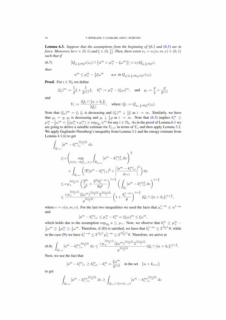
Lemma 6.3. Suppose that the assumptions from the beginning of §6.1 and (6.3) are inforce. Moreover, let ν ∈ (0, 1) and ξ ∈ (0, 1

2 ]. Then, there exists ν1 = ν1(n,m, ν) ∈ (0, 1)such that if

(6.7)∣∣Q%, 12νθ%2(zo) ∩

um > µm+ − ξωm

∣∣ < ν1|Q%, 12νθ%2 |,

thenum ≤ µm+ − 1

2ξωm a.e. in Q%/2, 12νθ(%/2)2(zo).

Proof. For i ∈ N0 we define

(ξi)m :=

1

2ξ +

1

2i+1ξ, kmi := µm+ − (ξiω)m, and %i :=

%

2+

%

2i+1

and

Yi :=|Qi ∩ u > ki|

|Qi|, where Qi := Q%i, 12νθ%2

i(zo).

Note that (ξo)m = ξ, ξi is decreasing and (ξi)

m ↓ 12ξ as i → ∞. Similarly, we have

that %o = %, %i is decreasing and %i ↓ 12% as i → ∞. Note that (6.3) implies kmi ≥

µm+ − 12ω

m = 12 (µm+ +µm− ) ≥ supQ0

ψm for any i ∈ N0. As in the proof of Lemma 6.1 weare going to derive a suitable estimate for Yi+1 in terms of Yi, and then apply Lemma 3.2.We apply Gagliardo-Nirenberg’s inequality from Lemma 3.1 and the energy estimate fromLemma 4.1 (i) to get∫

Qi+1

[um − kmi ]2(n+2)n

+ dz

≤ c

(sup

t∈(to−θ%2i+1,to)

∫B%i+1

[um − kmi ]2+ dx

) 2n

×∫Qi+1

(|∇[um − kmi ]+|2 +

∣∣∣∣ [um − kmi ]+%i+1

∣∣∣∣2)dz

≤ c µ2(m−1)

n+

(22i

%2+

22ik1−mi

θ%2

)1+ 2n(∫

Qi

[um − kmi ]2+ dz

)1+ 2n

≤c µ

2(m−1)n

+ (ξωm)2(n+2)n 2

2i(n+2)n

%2(n+2)n

(1 +

k1−mi

θ

)1+ 2n

|Qi ∩ u > ki|1+ 2n ,

where c = c(n,m, ν). For the last two inequalities we used the facts that µ1−m+ ≤ u1−m

and[um − kmi ]+ ≤ µm+ − kmi = (ξiω)m ≤ ξωm,

which holds due to the assumption supQ0u ≤ µ+. Now, we observe that kmi ≥ µm+ −

12ω

m ≥ 12µ

m+ ≥ 1

2ωm. Therefore, if (D) is satisfied, we have that k1−m

i ≤ 2m−1m θ, while

in the case (N) we have k1−mi ≤ 2

m−1m µ1−m

+ ≤ 2m2−1m θ. Therefore, we arrive at∫

Qi+1

[um − kmi ]2(n+2)n

+ dz ≤c µ

2(m−1)n

+ (ξωm)2(n+2)n 2

2i(n+2)n

%2(n+2)n

|Qi ∩ u > ki|1+ 2n .(6.8)

Next, we use the fact that

[um − kmi ]+ ≥ kmi+1 − kmi =ξωm

2i+2in the set u > ki+1

to get ∫Qi+1

[um − kmi ]2(n+2)n

+ dz ≥∫Qi+1∩u>ki+1

[um − kmi ]2(n+2)n

+ dz


≥ (ξωm)2(n+2)n

42(n+2)n 2

2i(n+2)n

|Qi+1 ∩ u > ki+1|.

Combining the last estimate with (6.8), we get

|Qi+1 ∩ u > ki+1| ≤c 4

2i(n+2)n µ

2(m−1)n

+

%2(n+2)n

|Qi ∩ u > ki|1+ 2n ,

where, again, c = c(n,m, ν). Dividing both sides by |Qi+1| and recalling the definition ofYi, we get

Yi+1 ≤c biµ

2(m−1)n

+ |Qi|1+ 2n

%2(1+ 2n )|Qi+1|

Y1+ 2

ni ,

where we abbreviated b := 42(n+2)n . If (D) is satisfied, we have that µm+ = 2µm+ − µm+ ≤

2µm+ − 2µm− = 2ωm = 2θm

1−m , while in the case that (N) is satisfied we have µm+ ≤2mθ

m1−m . Taking also into account that 1

2% ≤ %i ≤ % for all i ∈ N, we obtain

Yi+1 ≤ c biYi,

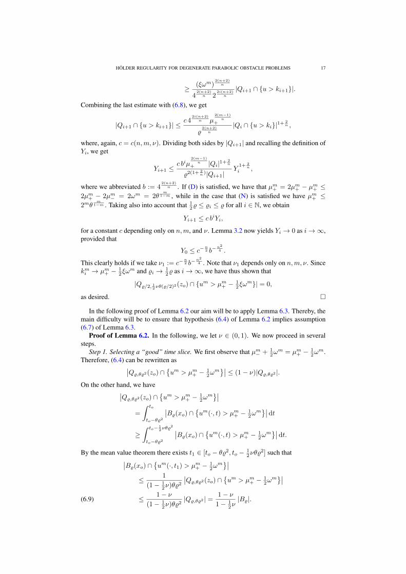
for a constant c depending only on n,m, and ν. Lemma 3.2 now yields Yi → 0 as i→∞,provided that

Y0 ≤ c−n2 b−

n2

4 .

This clearly holds if we take ν1 := c−n2 b−

n2

4 . Note that ν1 depends only on n,m, ν. Sincekmi → µm+ − 1

2ξωm and %i → 1

2% as i→∞, we have thus shown that

|Q%/2, 12νθ(%/2)2(zo) ∩ um > µm+ − 12ξω

m| = 0,

as desired.

In the following proof of Lemma 6.2 our aim will be to apply Lemma 6.3. Thereby, themain difficulty will be to ensure that hypothesis (6.4) of Lemma 6.2 implies assumption(6.7) of Lemma 6.3.

Proof of Lemma 6.2. In the following, we let ν ∈ (0, 1). We now proceed in severalsteps.

Step 1. Selecting a “good” time slice. We first observe that µm− + 12ω

m = µm+ − 12ω

m.Therefore, (6.4) can be rewritten as∣∣Q%,θ%2(zo) ∩

um > µm+ − 1

2ωm∣∣ ≤ (1− ν)|Q%,θ%2 |.

On the other hand, we have∣∣Q%,θ%2(zo) ∩um > µm+ − 1

2ωm∣∣

=

∫ to

to−θ%2

∣∣B%(xo) ∩ um(·, t) > µm+ − 12ω

m∣∣dt

≥∫ to− 1

2νθ%2

to−θ%2

∣∣B%(xo) ∩ um(·, t) > µm+ − 12ω

m∣∣dt.

By the mean value theorem there exists t1 ∈ [to − θ%2, to − 12νθ%

2] such that∣∣B%(xo) ∩ um(·, t1) > µm+ − 12ω

m∣∣

≤ 1

(1− 12ν)θ%2

∣∣Q%,θ%2(zo) ∩um > µm+ − 1

2ωm∣∣

≤ 1− ν(1− 1

2ν)θ%2|Q%,θ%2 | = 1− ν

1− 12ν|B%|.(6.9)


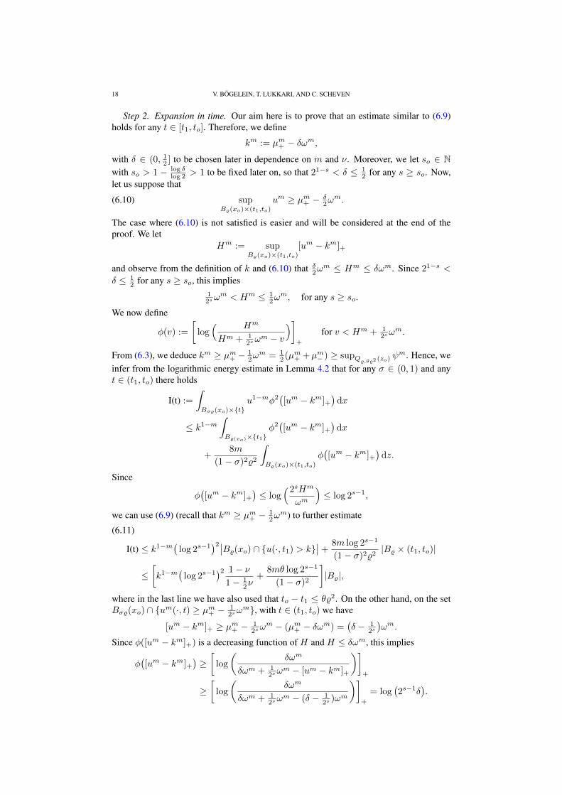
Step 2. Expansion in time. Our aim here is to prove that an estimate similar to (6.9)holds for any t ∈ [t1, to]. Therefore, we define

km := µm+ − δωm,

with δ ∈ (0, 12 ] to be chosen later in dependence on m and ν. Moreover, we let so ∈ N

with so > 1 − log δlog 2 > 1 to be fixed later on, so that 21−s < δ ≤ 1

2 for any s ≥ so. Now,let us suppose that

(6.10) supB%(xo)×(t1,to)

um ≥ µm+ − δ2ω

m.

The case where (6.10) is not satisfied is easier and will be considered at the end of theproof. We let

Hm := supB%(xo)×(t1,to)

[um − km]+

and observe from the definition of k and (6.10) that δ2ωm ≤ Hm ≤ δωm. Since 21−s <

δ ≤ 12 for any s ≥ so, this implies

12sω

m < Hm ≤ 12ω

m, for any s ≥ so.We now define

φ(v) :=

[log( Hm

Hm + 12sω

m − v

)]+

for v < Hm + 12sω

m.

From (6.3), we deduce km ≥ µm+ − 12ω

m = 12 (µm+ +µm− ) ≥ supQ%,θ%2 (zo) ψ

m. Hence, weinfer from the logarithmic energy estimate in Lemma 4.2 that for any σ ∈ (0, 1) and anyt ∈ (t1, to) there holds

I(t) :=

∫Bσ%(xo)×t

u1−mφ2([um − km]+

)dx

≤ k1−m∫B%(xo)×t1

φ2([um − km]+

)dx

+8m

(1− σ)2%2

∫B%(xo)×(t1,to)

φ([um − km]+

)dz.

Since

φ([um − km]+

)≤ log

(2sHm

ωm

)≤ log 2s−1,

we can use (6.9) (recall that km ≥ µm+ − 12ω

m) to further estimate

I(t) ≤ k1−m( log 2s−1)2∣∣B%(xo) ∩ u(·, t1) > k

∣∣+8m log 2s−1

(1− σ)2%2|B% × (t1, to)|

(6.11)

≤[k1−m( log 2s−1

)2 1− ν1− 1

2ν+

8mθ log 2s−1

(1− σ)2

]|B%|,

where in the last line we have also used that to − t1 ≤ θ%2. On the other hand, on the setBσ%(xo) ∩ um(·, t) ≥ µm+ − 1

2sωm, with t ∈ (t1, to) we have

[um − km]+ ≥ µm+ − 12sω

m − (µm+ − δωm) =(δ − 1

2s

)ωm.

Since φ([um − km]+) is a decreasing function of H and H ≤ δωm, this implies

φ([um − km]+

)≥[

log

(δωm

δωm + 12sω

m − [um − km]+

)]+

≥[

log

(δωm

δωm + 12sω

m − (δ − 12s )ωm

)]+

= log(2s−1δ

).


Therefore, we get the following lower bound for I(t):

I(t) ≥ µ1−m+

(log(2s−1δ

))2∣∣Bσ%(xo) ∩ um(·, t) ≥ µm+ − 12sω

m∣∣(6.12)

for all t ∈ (t1, to). Joining (6.11) and (6.12) yields∣∣Bσ%(xo) ∩ um(·, t) ≥ µm+ − 12sω

m∣∣

≤µm−1

+

(log(2s−1δ))2

[k1−m( log 2s−1

)2 1− ν1− 1

2ν+

8mθ log 2s−1

(1− σ)2

]|B%|,

for all t ∈ (t1, to). At this point, we use that km = (1 − δ)µm+ + δµm− ≥ (1 − δ)µm+ .Moreover, if (D) is satisfied, then ωm = µm+ − µm− ≥ 1

2µm+ and hence θ ≤ 2µ1−m

+ , whilein the case (N) we have θ ≤ 2m−1µ1−m

+ . Taking also into account that |B% \ Bσ%| =(1− σn)|B%| ≤ n(1− σ)|B%|, we can further estimate∣∣B%(xo) ∩ um(·, t) ≥ µm+ − 1

2sωm∣∣

≤[(1− δ)

1−mm

(log 2s−1

log(2s−1δ)

)21− ν

1− 12ν

+2m+3m log 2s−1

(1− σ)2(log(2s−1δ))2+ n(1− σ)

]|B%|.

We now choose

σ := 1− ν2

8n∈ (0, 1),

and

(6.13) δ := min

1

2, 1−

( 1− ν2

1− 12ν

2

) mm−1

≤ 1

2,

and note that

(1− δ)1−mm ≤

1− 12ν

2

1− ν2.

Then, the last inequality yields that∣∣B%(xo) ∩ um(·, t) ≥ µm+ − 12sω

m∣∣

≤[(

log 2s−1

log(2s−1δ)

)2 1− 12ν

2

(1− 12ν)(1 + ν)

+2m+9n2m log 2s−1

ν4(log(2s−1δ))2+ν2

8

]|B%|,

for any t ∈ (t1, to). Next, we choose so in dependence on n,m and ν large enough toensure that (

log 2so−1

log(2so−1δ)

)2

≤ (1 + ν)(1− 12ν)

and2m+9n2m log 2so−1

(log(2so−1δ))2≤ ν6

8

holds true. Then, we have for any s ≥ so and any t ∈ (t1, to) that∣∣B%(xo) ∩ um(·, t) ≥ µm+ − 12sω

m∣∣ ≤ ((1− 1

2ν2) + 1

4ν2)|B%| =

(1− 1

4ν2)|B%|,

provided that (6.10) is satisfied. On the other hand, if (6.10) is not satisfied, then we havethat ∣∣B%(xo) ∩ um(·, t) ≥ µm+ − δ

2ωm∣∣ = 0

holds true for any t ∈ [t1, to]. Since δ2 > 1

2s for any s ≥ so, this implies the second lastinequality. Therefore, in any case we have proved that there exists so = so(n,m, ν) ∈ N≥2

such that ∣∣B%(xo) ∩ um(·, t) ≥ µm+ − 12sω

m∣∣ ≤ (1− 1

4ν2)|B%|,

or equivalently

(6.14)∣∣B%(xo) ∩ um(·, t) < µm+ − 1

2sωm∣∣ ≥ 1

4ν2|B%|,

holds true for any t ∈ [t1, to] and any s ≥ so.


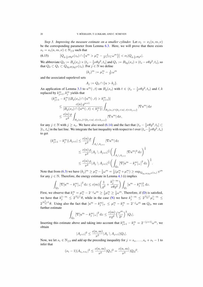
Step 3. Improving the measure estimate on a smaller cylinder. Let ν1 = ν1(n,m, ν)be the corresponding parameter from Lemma 6.3. Here, we will prove that there existss1 = s1(n,m, ν) ∈ N≥2 such that

(6.15)∣∣Q%, 12νθ%2(zo) ∩

um > µm+ − 1

2so+s1ωm∣∣ < ν1|Q%, 12νθ%2 |.

We abbreviate Q2 := B%(xo)× (to− 12νθ%

2, to] and Q1 := B2%(xo)× (to− νθ%2, to], sothat Q2 ⊂ Q1 ⊂ Q2%,θ(2%)2(zo). For j ∈ N we define

(kj)m := µm+ − 1

2j ωm

and the associated superlevel sets

Aj := Q2 ∩ u > kj.An application of Lemma 3.3 to um(·, t) on B%(xo) with t ∈ (to − 1

2νθ%2, to) and `, k

replaced by kmj+1, kmj yields that

(kmj+1 − kmj )|B%(xo) ∩ um(·, t) > kmj+1|

≤ c(n) %n+1

|B%(xo) ∩ um(·, t) < kmj |

∫B%(xo)∩kj<u(·,t)<kj+1

|∇um|dx

≤ c(n) %

ν2

∫B%(xo)∩kj<u(·,t)<kj+1

|∇um|dx,

for any j ∈ N with j ≥ so. We have also used (6.14) and the fact that (to − 12νθ%

2, to] ⊂[t1, to] in the last line. We integrate the last inequality with respect to t over (to− 1

2νθ%2, to)

to get

(kmj+1 − kmj )|Aj+1| ≤c(n) %

ν2

∫Aj\Aj+1

|∇um|dz

≤ c(n) %

ν2|Aj \Aj+1|

12

(∫Aj\Aj+1

|∇um|2 dz

) 12

≤ c(n) %

ν2|Aj \Aj+1|

12

(∫Q2

∣∣∇[um − kmj ]+∣∣2 dz

) 12

.

Note that from (6.3) we have (kj)m ≥ µm+ − 1

2ωm = 1

2 (µm+ +µm− ) ≥ supQ2%,θ(2%)2 (zo) ψm

for any j ∈ N. Therefore, the energy estimate in Lemma 4.1 (i) implies∫Q2

∣∣∇[um − kmj ]+∣∣2 dz ≤ c(m)

(1

%2+k1−mj

νθ%2

)∫Q1

[um − kmj ]2+ dz.

First, we observe that kmj = µm+ − 2−jωm ≥ 12µ

m+ ≥ 1

2ωm. Therefore, if (D) is satisfied,

we have that k1−mj ≤ 2

m−1m θ, while in the case (N) we have k1−m

j ≤ 2m−1m µ1−m

+ ≤

2m2−1m θ. Using also the fact that [um − kmj ]+ ≤ µm+ − kmj = 2−jωm on Q2, we can

further estimate ∫Q2

∣∣∇[um − kmj ]+∣∣2 dz ≤ c(m)

ν%2

(ωm2j

)2

|Q1|.

Inserting this estimate above and taking into account that kmj+1 − kmj = 2−(j+1)ωm, weobtain

|Aj+1|2 ≤c(n,m)

ν5|Aj \Aj+1||Q1|.

Now, we let s1 ∈ N≥2 and add up the preceding inequality for j = so, . . . , so + s1 − 1 toinfer that

(s1 − 1)|Aso+s1 |2 ≤c(n,m)

ν5|Q1|2 =

c(n,m)

ν5|Q2|2.


Choosing s1 = s1(n,m, ν, ν1) ≡ s1(n,m, ν) large enough to ensure that

c(n,m)

ν5(s1 − 1)≤ ν2

1 ,

we conclude the claim (6.15).Step 4. Concluding the proof of Lemma 6.2. Due to (6.15) we are allowed to apply

Lemma 6.3 with ξ = 2−(so+s1) to conclude that

um ≤ µm+ − 12ξω

m a.e. in Q%/2, 12νθ(%/2)2(zo).

This proves the assertion of Lemma 6.2 for the choice a = 12ξ. Note that ξ depends on

n,m, ν and therefore the parameter a depends on the same quantities. Combining the two alternatives (Lemma 6.1 and Lemma 6.2) we get the following

proposition.

Proposition 6.4. Suppose that the assumptions from the beginning of §6.1 are in force andlet Q2%,θ(2%)2(zo) ⊂ ΩT be a parabolic cylinder satisfying

infQ2%,θ(2%)2 (zo)

u ≥ µ−, supQ2%,θ(2%)2 (zo)

u ≤ µ+, and supQ2%,θ(2%)2 (zo)

ψm ≤ 12

(µm+ + µm−

).

Then, there exists νo = νo(n,m) ∈ (0, 1) and a = a(n,m) ∈ (0, 14 ] such that either

infQ%/2,θ(%/2)2 (zo)

um ≥ µm− + 14ω

m, or supQ%/2, 1

2νoθ(%/2)2

(zo)

um ≤ µm+ − aωm

holds true.

Proof. We let νo = νo(n,m) ∈ (0, 1) be the constant from Lemma 6.1. Then we takea = a(n,m, νo) ≡ a(n,m) ∈ (0, 1

4 ] to be the constant from Lemma 6.2 applied withν = νo. With these choices, one of the alternatives (6.2) and (6.4) of Lemmas 6.1 and 6.2is satisfied for the given cylinder. Therefore, the application of Lemma 6.1, respectivelyLemma 6.2 yields the claim.

6.2. The degenerate and the nondegenerate regime. In this section we constructsmaller cylinders on which the oscillation is reduced. We need to treat the two differentregimes introduced at the beginning of §6.1 separately.

Throughout this subsection we let νo = νo(n,m) ∈ (0, 1) and a = a(n,m) ∈ (0, 14 ] be

the constants from Proposition 6.4 and define δ := 1− a ∈ [ 34 , 1).

We start by considering the degenerate regime. Here, we prove a reduction of the os-cillation of um on a smaller cylinder. Since we do not know if the smaller cylinder againbelongs to the degenerate regime, we cannot iterate the argument.

Proposition 6.5. Let µ−, µ+ ≥ 0 be two parameters with

(6.16) µ− ≤ 12µ+

and defineθ := ω1−m with ωm := µm+ − µm− .

Suppose that Q := Q%,θ%2(zo) ⊂ ΩT is a parabolic cylinder satisfying

infQu ≥ µ−, sup

Qu ≤ µ+, and sup

Qψm ≤ 1

2

(µm+ + µm−

).

Then, with

(ω1)m := maxδωm, 2 osc

Qψm,

and

Q1 := Q%1,θ1%21(zo), where θ1 := ω1−m

1 , %1 := η%, η :=

√132νoδ

m−1m ,


there holds

(6.17) oscQ1

um ≤ ωm1 , and Q1 ⊂ Q.

Proof. First, we observe that η < 14δ

m−12m < 1

4 and ω1 ≥ δ1mω, which implies that

(6.18) Q1 ⊂ Q%/4, 12νoθ(%/4)2(zo) ⊂ Q%/4,θ(%/4)2(zo) ⊂ Q.

Moreover, we note that assumption (D) is satisfied. Therefore, we can apply Proposi-tion 6.4 to conclude that either

infQ%/4,θ(%/4)2 (zo)

um ≥ µm− + 14ω

m, or supQ%/4, 1

2νoθ(%/4)2

(zo)


holds true. By (6.18), this implies that either

infQ1

um ≥ µm− + 14ω

m, or supQ1


is satisfied. If the first alternative occurs, we conclude

oscQ1

um = supQ1

um − infQ1

um ≤ µm+ − (µm− + 14ω

m) = (1− 14 )ωm ≤ δωm ≤ ωm1 ,

while in the case that the second alternative occurs, we have that

oscQ1

um = supQ1

um − infQ1

um ≤ µm+ − aωm − µm− = (1− a)ωm = δωm ≤ ωm1 .

This proves the assertion of the proposition.

Next, we consider the nondegenerate regime. As in the degenerate regime, we can provea reduction of the oscillation on a smaller cylinder. However, in contrast to the degenerateregime, we can even prove that the smaller cylinder again belongs to the nondegenerateregime. Therefore, we can use an induction argument to prove a reduction of the oscillationon a sequence of concentric nested cylinders.

Proposition 6.6. Let νo = νo(n,m) ∈ (0, 1) and δ = δ(n,m) ∈ (0, 1) be the constantsfrom the beginning of §6.2 and let 0 < µ− ≤ µ+ be two parameters satisfying

µ− >12µ+

and define θ := µ1−m+ . Suppose that Qo := Q%o,θ%2

o(zo) ⊂ ΩT is a parabolic cylinder

satisfyinginfQou ≥ µ− and sup

Qo

u ≤ µ+,

as well as

(6.19) supQo

ψm ≤ 12

(µm+ + µm−

)and osc

Qoψm ≤ 1

2

(µm+ − µm−

).

With the sequence of cylinders

Qi := Q%i,θ%2i(zo), where %i := ηi%o, η :=

√132νo ,

we define

(ωo)m := µm+ − µm− , and (ωi)

m := maxδωmi−1, 2 osc

Qi−1

ψm

for i ∈ N.

Then, for any i ∈ N0 there holds

(6.20) oscQi

um ≤ ωmi .


Proof. First, we observe that

(6.21) Qi+1 ⊂ Q%i/4, 12νoθ(%i/4)2(zo) ⊂ Q%i/4,θ(%i/4)2(zo) ⊂ Qi, for any i ∈ N0.

Next, we define µ−,o := µ− and µ+,o := µ+, as well as

µ−,i := infQiu, µm+,i := µm−,i + ωmi , for i ∈ N.

From (6.19) and the definition of ω1, we deduce ω1 ≤ ωo. Then, we infer inductively that

(6.22) ωi+1 ≤ ωi for all i ∈ N0.

Next, we note that

(6.23) (2µ+,i)1−m ≤ θ ≤ ( 1

2µ+,i)1−m

holds for any i ∈ N0. In fact, the first inequality is a consequence of θ = µ1−m+,o ≥

(2µ−,o)1−m ≥ (2µ−,i)

1−m ≥ (2µ+,i)1−m, while the second follows from µm+,i = µm−,i +

ωmi ≤ supQo um + ωmo ≤ 2µm+,o = 2θ

m1−m . Moreover, we have for any i ∈ N

supQi

ψm = infQiψm + osc

Qiψm ≤ inf

Qium + osc

Qi−1

ψm ≤ µm−,i + 12ω

mi = 1

2 (µm+,i + µm−,i),

while for i = 0, the same holds by assumption (6.19)1.In the following, we will prove

(6.24)

µ−,i >

12µ+,i

oscQi um ≤ ωmi ,

for any i ∈ N0 by induction. For i = 0 the assertion (6.24) is a direct consequence ofthe assumptions on µ− and µ+. We now assume that (6.24) is satisfied for some i ∈ N0.Keeping in mind (6.22) and µ−,i ≤ µ−,i+1, we deduce

µm+,i+1 = µm−,i+1 + ωmi+1 = 2mµm−,i+1 +(ωmi+1 − (2m − 1)µm−,i+1

)≤ 2mµm−,i+1 +

(ωmi − (2m − 1)µm−,i

)= 2mµm−,i+1 + (µm+,i − 2mµm−,i)

< 2mµm−,i+1,

which proves the first assertion in (6.24) for i+ 1. Moreover, we have that µm+,i = µm−,i +ωmi ≥ supQi u

m and hence µ+,i ≥ supQi u and assumption (N) holds for Qi by (6.24)1and (6.23). Therefore, we can apply Proposition 6.4 to conclude that either

infQ%i/4,θ(%i/4)2 (zo)

um ≥ µm−,i + 14ω

mi , or sup

Q%i/4, 1

2νoθ(%i/4)2

(zo)

um ≤ µm+,i − aωmi

holds true. By the inclusions (6.21), this implies that either

infQi+1

um ≥ µm−,i + 14ω

mi , or sup

Qi+1

um ≤ µm+,i − aωmi

holds true. If the first alternative occurs, we conclude

oscQi+1

um = supQi+1

um − infQi+1

um ≤ µm+,i − (µm−,i + 14ω

mi )

= (1− 14 )ωmi ≤ δωmi ≤ ωmi+1,

while in the case that the second alternative occurs, we have that

oscQi+1

um = supQi+1

um − infQi+1

um ≤ µm+,i − aωmi − µm−,i

= (1− a)ωmi = δωmi ≤ ωmi+1.

Hence, in both cases we have proved (6.24)2 and thereby (6.20) for i+ 1. This finishes theproof of the proposition.


6.3. The final iteration. In this section we finally prove the Holder continuity of the so-lution to the obstacle problem for the porous medium equation. For this aim, we let

ε :=2β(m− 1)

2m+ β(m− 1)∈ (0, 1) and γo :=

2βm

2m+ β(m− 1)∈ (0, 1),

where β ∈ (0, 1) is the Holder exponent from assumption (6.1). Then, we fix zo ∈ ΩT andconsider R ∈ (0, 1) such that Q2R,4R2−ε(zo) ⊂ ΩT . If

oscQ%,%2−ε (zo)

um ≤ max%εmm−1 , 2 osc

Q%,%2−ε (zo)ψm

=: Ψ(%), for any % ∈ (0, R],

we use the Holder continuity assumption (6.1) on ψ and the choice of ε to see that

Ψ(%) ≤ c max%εmm−1 , %β−

εβ2

= c %γo , for any % ∈ (0, R],

so that um is Holder continuous at zo. Therefore, it remains to consider the remaining case.In this case we either have for %o = R that

Ψ(%o) < oscQ%o,%

2−εo

(zo)um ≤ ‖u

m‖L∞Rγo

%γoo ,

or we can find a %o ∈ (0, R) with

oscQ%o,%

2−εo

(zo)um > Ψ(%o), and osc

Qr,r2−ε (zo)um ≤ 2Ψ(r) for any r ∈ [%o, R].

With this choice of %o, we define

µ−,o := infQ%o,%

2−εo

(zo)u, µ+,o := sup

Q%o,%

2−εo

(zo)

u

andωmo := µm+,o − µm−,o and θo := ω1−m

o .

With these choices of parameters, we have

θo = ω1−mo =

(osc

Q%o,%

2−εo

(zo)um) 1−m

m

< Ψ(%o)1−mm ≤ %−εo ,

so that Qo := Q%o,θo%2o(zo) ⊂ Q%o,%2−ε

o(zo). Therefore, we find that

supQo

ψm ≤ supQ%o,%

2−εo

(zo)

ψm = infQ%o,%

2−εo

(zo)ψm + osc

Q%o,%

2−εo

(zo)ψm(6.25)

≤ infQ%o,%

2−εo

(zo)um + 1

2 oscQ%o,%

2−εo

(zo)um = µm−,o + 1

2

(µm+,o − µm−,o

)= 1

2

(µm+,o + µm−,o

).

By νo, δ ∈ (0, 1) we denote the corresponding constants from the beginning of §6.2, bothdepending only on n and m. We define sequences of nonnegative numbers ωi, µ+,i, µ−,i,and cylinders Qi for i ∈ N by the following recursive scheme. Assuming that ωi−1 andQi−1 have already been defined, we let

(ωi)m := max

δωmi−1, 2 osc

Qi−1

ψm,

andµ−,i := inf

Qiu, µm+,i := µm−,i + ωmi ,

as well as

Qi := Q%i,θi%2i(zo), with θi := ω1−m

i , %i := ηi%o, η :=

√132νoδ

m−1m .

For any i ∈ N, we deduce

(6.26) supQi

ψm = infQiψm + osc

Qiψm ≤ inf

Qium + 1

2ωmi = 1

2 (µm+,i + µm−,i).


We let io be the first index for which Qio is in the nondegenerate regime, i.e. we chooseio ∈ N0 ∪ ∞ in such a way that µ−,io >

12µ+,io and µ−,i ≤ 1

2µ+,i for any i < io. Ifµ−,i ≤ 1

2µ+,i for any i ∈ N0, we set io = ∞. We will apply Proposition 6.5 to prove byinduction that

(6.27) Qio ⊂ Qio−1 ⊂ · · · ⊂ Qo, and oscQi

um ≤ ωmi ,

for any i ∈ 0, . . . , io, (resp. i ∈ N0 if io = ∞). For i = 0 the assertion (6.27) isa direct consequence of the definition of ωo. If io = 0, we are finished and therefore itremains to consider the case where io > 0. We now assume that (6.27) is satisfied forsome i ∈ 0, . . . , io − 1. Then, we have µm+,i = µm−,i + ωmi ≥ supQi u

m and henceµ+,i ≥ supQi u. Moreover, we have supQi ψ

m ≤ 12 (µm+,i + µm−,i) by (6.26), respectively

by (6.25). Therefore, we can apply Proposition 6.5 on the cylindersQi to infer thatQi+1 ⊂Qi and

oscQi+1

um ≤ ωmi+1.

This proves the claim (6.27).If io < ∞, we redefine the remaining cylinders so that Proposition 6.6 can be applied.

Let θ∗ := µ1−m+,io

≤ θio and redefine the cylinders for i ∈ io + 1, . . . by

Qi := Q%i,θ∗%2i(zo), with %i := ηi−io%io , η :=

√132νo.

Note that Qio ⊃ Qio+1 ⊃ . . . and that the redefinition of Qi also leads to a redefinition ofωi, µ−,i and µ+,i.

Our aim is to apply Proposition 6.6 on the cylinder Q∗io := Q%io ,θ∗%2io

(zo) ⊂ Qio , withthe parameters µ+,io and µ−,io . To this end, we check that

infQ∗io

u ≥ infQio

u = µ−,io and supQ∗io

u ≤ supQio

u ≤ µ+,io .

Moreover, from (6.26), respectively from (6.25), we know

supQ∗io

ψm ≤ supQio

ψm ≤ 12 (µ+,io + µ−,io),

and the definition of ωio , respectively the choice of %o, implies

µm+,io − µm−,io = ωmio ≥ 2 osc

Qioψm ≥ 2 osc

Q∗io

ψm.

Hence, Proposition 6.6 is applicable on Q∗io and provides us with the estimate

(6.28) oscQi

um ≤ ωmi , for any i ∈ io + 1, . . . .

For i ∈ N0 we now define

ri := min

1, ω1−m

2o

%i,

so thatQri(zo) := Qri,r2

i(zo) ⊂ Qi, for any i ∈ N0.

Therefore, for any i ∈ N0 we can use either (6.27), or (6.28) to conclude that

oscQri

um ≤ oscQi

um ≤ ωmi ≤ δωmi−1 + 2 oscQi−1

ψm ≤ δiωmo + 2

i−1∑j=0

δj oscQi−1−j

ψm.

In the case i− 1− j ≤ io, we infer from assumption (6.1) that

oscQi−1−j

ψm ≤ c(%βi−1−j + (θi−1−j%

2i−1−j)

β2

)= c(1 + ω

β(1−m)2

i−1−j)%βi−1−j

≤ c(1 + (δ

i−1−jm ωo)

β(1−m)2

)%βi−1−j ≤ c

(1 + ω

β(1−m)2

o

)δ

(i−1−j)β(1−m)2m %βi−1−j

= c(1 + ω

β(1−m)2

o

)(νo32

) β(i−1−j)2 %βo .


For i− 1− j > io we get the same bound, since

oscQi−1−j

ψm ≤ c(%βi−1−j + (θ∗%

2i−1−j)

β2

)≤ c(1 + ω

β(1−m)2

io

)%βi−1−j

≤ c(1 + (δ

iom ωo)

β(1−m)2

)%βi−1−j ≤ c

(1 + ω

β(1−m)2

o

)δioβ(1−m)

2m %βi−1−j

= c(1 + ω

β(1−m)2

o

)(νo32

) β(i−1−j)2 %βo .

Inserting this above, we conclude for any i ∈ N0 that

oscQri

um ≤ δiωmo + c(1 + ω

β(1−m)2

o

)%βo

i−1∑j=0

δj(νo32

) β(i−1−j)2 .

With the abbreviation

κ := maxδ,(νo32

) β2

this shows that

oscQri

um ≤ δiωmo + c iκi−1(1 + ω

β(1−m)2

o

)%βo .

Since i√κi ≤ −2/(e log κ), this leads us to

oscQri

um ≤ δiωmo + c√κi(

1 + ωβ(1−m)

2o

)%βo ,

for a constant c depending only on n,m, β, and [ψ]0;β,β/2. Now, we define

γ1 := min log κ

2 log η, γo

and note that γ1 ≤ log δ

log η . Therefore, from the last inequality and the fact ηi ≤ %i%o

weconclude that

oscQri

um ≤ ηγ1iωmo + c ηγ1i(1 + ω

β(1−m)2

o

)%βo(6.29)

≤ c(n,m, β, [ψ]0;β,β/2, ‖u‖L∞ , R) rγ1

i .

Now, we consider r ∈ (0, R]. If r ∈ (0, ro) we choose i ∈ N0 such that ri+1 ≤ r < ri.Then, from (6.29) we have

oscQr

um ≤ oscQri

um ≤ c rγ1

i ≤ c η−γ1rγ1 .

Otherwise, if r ∈ [ro, %o), we estimate

oscQr

um ≤ oscQ%o,%

2−εo

um ≤ 2Ψ(%o) ≤ c(r%o

)γ1Ψ(%o) ≤ c rγ1 .

Finally, by the choice of %o we have for r ∈ [%o, R] that

oscQr

um ≤ oscQr,r2−ε

um ≤ 2Ψ(r) ≤ c rγo ≤ c rγ1 .

Therefore, we conclude that um is Holder continuous at zo. Since zo ∈ ΩT was arbitrary,this proves that um, and hence also u, is locally Holder continuous in ΩT . This finishesthe proof of Theorem 1.1.


REFERENCES

[1] H. Alt and S. Luckhaus. Quasilinear elliptic-parabolic differential equations. Math. Z., 183(3):311–341,1983.

[2] B. Avelin and T. Lukkari. A comparison principle for the porous medium equation and its consequences.Submitted. Available at http://arxiv.org/abs/1505.07579.

[3] V. Bogelein, F. Duzaar and U. Gianazza. Continuity estimates for porous medium type equations withmeasure data. J. Funct. Anal., 267:3351–3396, 2014.

[4] V. Bogelein, F. Duzaar, and G. Mingione. Degenerate problems with irregular obstacles. J. Reine Angew.Math., 650:107–160, 2011.

[5] V. Bogelein, T. Lukkari, C. Scheven. The obstacle problem for the porous medium equation. Math. Ann.,DOI 10.1007/s00208-015-1174-3.

[6] V. Bogelein and C. Scheven. Higher integrability in parabolic obstacle problems. Forum Math., 24(5):931–972, 2012.

[7] P. Daskalopoulos and C. E. Kenig. Degenerate diffusions – Initial value problems and local regularity the-ory. European Mathematical Society (EMS), Zurich, 2007.

[8] E. DiBenedetto. Degenerate Parabolic Equations. Springer Universitext, Springer, New York, 1993.[9] E. DiBenedetto, U. Gianazza and V. Vespri, Harnack’s inequality for degenerate and singular parabolic

equations. Springer Monographs in Mathematics. Springer, New York, 2012.[10] E. DiBenedetto and A. Friedman. Holder estimates for nonlinear degenerate parabolic systems. J. Reine

Angew. Math., 357:1–22, 1985.[11] E. Giusti, Direct Methods in the Calculus of Variations. World Scientific, Singapore, 2003.[12] R. Korte, T. Kuusi, and J. Siljander. Obstacle problem for nonlinear parabolic equations. J. Differential

Equations, 246(9):3668–3680, 2009.[13] P. Lindqvist and M. Parviainen. Irregular time dependent obstacles. J. Funct. Anal., 263(8):2458–2482,

2012.[14] J.-L. Lions. Quelques methodes de resolution des problemes aux limites non lineaires. Dunod, 1969.[15] J. Naumann. Einfuhrung in die Theorie parabolischer Variationsungleichungen, Volume 64 of Teubner-

Texte zur Mathematik. BSB B. G. Teubner Verlagsgesellschaft, Leipzig, 1984.[16] J. L. Vazquez. The porous medium equation – Mathematical theory. Oxford University Press, Oxford, 2007.[17] Z. Wu, J. Zhao, J. Yin, and H. Li. Nonlinear diffusion equations. World Scientific Publishing Co., Inc., River

Edge, NJ, 2001.

VERENA BOGELEIN, FACHBEREICH MATHEMATIK, UNIVERSITAT SALZBURG, HELLBRUNNER STR. 34,5020 SALZBURG, AUSTRIA

E-mail address: [email protected]

TEEMU LUKKARI, DEPARTMENT OF MATHEMATICS AND STATISTICS, P.O. BOX 35 (MAD), 40014UNIVERSITY OF JYVASKYLA, JYVASKYLA, FINLAND


CHRISTOPH SCHEVEN, FAKULTAT FUR MATHEMATIK, UNIVERSITAT DUISBURG-ESSEN, THEA-LEYMANN-STR. 9, 45127 ESSEN, GERMANY


http://arxiv.org/abs/1505.07579

HOLDER REGULARITY FOR DEGENERATE PARABOLIC OBSTACLE¨

Documents

Transcript of HOLDER REGULARITY FOR DEGENERATE PARABOLIC OBSTACLE¨