Hold-Up in the NFL: Team Specific investment in the National Football League

Darren King B.A., Wilfrid Laurier University

PROJECT SUBNITTED IN PARTIAL FULFILLMENT OF THE REQUIREMENTS FOR THE DEGREE OF

MASTER OF ARTS In The

Department of Ikonornics

O Darren King 2006

SIMON FRASER UNIVERSITY Spring 2006

All rights reserved. This work may not be reproduced in whole or in part, by photocopy or by other means,

without the permission of the author.

Name:

APPROVAL,

Darren King

Degree: M. A. (Economics)

Title of Project : Hold-Up In The NFL: Team Specific Investment In The National Football League

Examining Committee:

Chair: Ken Kasa

Christoph Luelfesmann Senior Supervisor

Simon Woodcock Supervisor

Phil Curry Internal Examiner

Date Approved: Thursday, April 6th, 2006

SIMON FRASER UNlVERslTYl i bra ry

DECLARATION OF PARTIAL COPYRIGHT LICENCE

The author, whose copyright is declared on the title page of this work, has granted to Simon Fraser University the right to lend this thesis, project or extended essay to users of the Simon Fraser University Library, and to make partial or single copies only for such users or in response to a request from the library of any other university, or other educational institution, on its own behalf or for one of its users.

The author has further granted permission to Simon Fraser University to keep or make a digital copy for use in its circulating collection, and, without changing the content, to translate the thesislproject or extended essays, if technically possible, to any medium or format for the purpose of preservation of the digital work.

The author has further agreed that permission for multiple copying of this work for scholarly purposes may be granted by either the author or the Dean of Graduate Studies.

It is understood that copying or publication of this work for financial gain shall not be allowed without the author's written permission.

Permission for public performance, or limited permission for private scholarly use, of any multimedia materials forming part of this work, may have been granted by the author. This information may be found on the separately catalogued multimedia material and in the signed Partial Copyright Licence.

The original Partial Copyright Licence attesting to these terms, and signed by this author, may be found in the original bound copy of this work, retained in the Simon Fraser University Archive.

Simon Fraser University Litlrary Burnaby, BC, Canada

Abstract

In a Nash bargaining scenario players will not be fully compensated for

investments in their own productivity which are not transferable between teams. This

paper constructs a model of NFL players' compensation to examine the optimal

investment level when there are both general and team specific investments. It is found

that specific investment will lead to less than optimal investment levels. Furthermore,

teams and players will be able to increase the optimal investment level by agreeing to an

initial contract. The model predicts that players i n positions that require a large specific

investment will find it optimal to agree to a long term contract in which a greater

proportion of the salary is paid in the first period. The model also predicts that players in

positions that require a large specific investmenl will switch teams less often. Using NFL

data I find evidence to support these predictions.

Keywords:

Specific Investment, Contracts, NFL

Acknowledgements

I would like to thank the faculty, staff and my fellow students in the Department

of Economics for their contribution to my understanding of and appreciation for

economics. I thank Prof. Christoph Liilfesmann for teaching an interesting and

informative class which led me to the creation of this paper, and for his many

contributions to theoretical model. I also thank Prof. Simon Woodcock for his assistance

with the empirical estimations. This paper would not have been possible without their

guidance and encouragement. I also thank Prof. Philip Curry for his willingness to

contribute and for his valuable feedback.

Contents ............................................................................................................... Approval ii

... Abstract ............................................................................................................... III Acknowledgements ............................... ............................................................. iv

Contents ............................................................................................................ v

List of Tables ....................................................................................................... vi

Introduction ..................................................................................................... - I - Incomplete Contracts and Contract Renegotiation ..................................... - 3 - Contracts, Renegotiation and Free Agency ................................................ - 6 -

.......................................................................................................... Renegotiation - 6 - Free Agency ............................................................................................................ - 7 -

Player Investment and the Determination of Salary .................................... - 9 - Contract Bargaining ...................................................................................... - I I - The Bargaining Model .................................................................................. - 13 -

.......................................................................................................... Assumptions - 13 - ......................................................................................... Possible Contingencies - 14 -

Solving the Model for First Best Investment Levels ........................................ - 17 - ........................................................................................ Equilibrium Investment - 18 -

Equilibrium Investment with an Initial Contract .................................................. - 19 - . . .............................................................................................................. Predictions 22 - Testing the Predictions of the Model ........................................................... - 24 - Description of the Data ................................................................................ - 25 -

....................................................................................... The Dependent Variable - 25 - ................................................................................... The Independent Variables - 25 -

Specificity .............................................................................................................. - 26 - ........................................................................................................... Old Dummy - 28 -

Estimation and Results ................................................................................ - 29 - ................................................................................................ Testing for Mobility 31 -

Conclusions ................................................................................................ - 34 - Tables and Regressions ........................................................................... - 35 - References .................................................................................................... - 43 -

List of Tables

Regression #1 ............................................................................................................... 29 -

Team Switchers by Specific and Non-Specific Positions ................................... - 32 -

. ......................................................................................................... Probit Regression 33

Table 1: Salary Cap Value by Position ...................................................................... 35 -

Table 2: Player Statistics ............................................................................................ 36 -

Table 3: Specific & Old Dummies ............................................................................. 36 -

Table 4: Average Salaries' Composition by Position 2004 ...................................... - 37 -

Table 5: Salary Cap by Year ...................................................................................... - 37 -

Table 6: Team Switchers and Experience by Position ............................................ 38 -

Regression #2 ............................................................................................................... 39 -

Regression #3 ............................................................................................................... - 40 -

. Regression #4 ............................................................................................................... - 42

Introduction

In 2003 the Denver Broncos acquired Jake Plurnmer as a fi-ee agent from the

Arizona Cardinals. The Broncos had spent the previous four years struggling to overcome

the retirement of their Hall of fame quarterback John Elway, who led the team to back-to-

back Super Bowl wins before retiring. Without Elway the team was unable to win a single

play-off game. Their supposed future star, who Ihad been learning the offense during

Elway's last season, suffered one hstration after another. With the acquisition of the

new quarterback there were big expectations in Denver. In his first two seasons with the

Broncos, Plummer was mediocre and the Broncos had limited success, once again failing

to win a play-off game. The 2005 season, however, was a different story for the Broncos.

Plurnrner had perhaps the best season of his career, was voted to the Pro-Bowl, and led

the Broncos deep into the post-season. When asked about the recent success o Chis

quarterback, coach Mike Shanahan replied that ]he had expected it would take three

seasons for Jake Plummer to learn the Broncos offensive system1.

In 2004 the Denver broncos traded away one of the league's top running backs to

Washington for cornerback Champ Bailey. Champ had a reputation as a "shut--down-

comer", referring to his ability to stop opposing receivers. Bailey's impact on the Broncos

defense was immediate. In his first season with the team he established himself as one of

the team's best defensive players. In his second season he set a new personal best for

interceptions, despite missing several games wilh injuries.

In 2005 Sports columnist Pete prisco2 observed that the quality of play from

offensive linemen around the league has not been as good as what we have come to

expect. Prisco attributed this decline in play to tlhe fi-ee agency era and the increased

mobility of players. The problem is that it takes an offensive line a long time to learn a

team's system and play competently as a unit. With players switching teams more

frequently there is less opportunity for a team to build an effective offensive line than

there was prior to free agency.

The same has not been true for defensive line play, and it is not the result of less

mobility among defensive linemen compared to their offensive counterparts. En 2005 the

1 Krieger, Dave. Rocky Mountain News Pete Prisco writes for www.cbssportsline.com

- 1 -

Denver Broncos shocked NFL observers by acquiring through trades and free agency,

almost the entire defensive line of the Cleveland Browns; a cast of underachievers if there

ever was one. Using some of these players to pa.tch holes in the Broncos startiing defense

resulted in the best line play the Broncos have had since the Super Bowl years.

All of these examples demonstrate the irnportance of team specific capital for

certain positions in the NFL. In the first instance, Bailey was able to switch defensive

systems with no loss in productivity, while Jake Plummer took three years to adjust to a

new system and a new set of receivers. In the second example, offensive line play has

arguably deteriorated because players do not have continued access to a team's system or

consistent teammates. The same problem has not occurred for defensive linemen.

But if players in some positions do make large team specific investments,

economic theory suggests that players at these plositions will not be hl ly compensated for

the efforts. This paper models an NFL labour contract, dependent on investments in

specific and general skills, and then tests the model's implications using NFL salary data.

Incomplete Contracts and Contract Renegotiation

This model of NFL contracts will follow the usual Principal-Agent framework.

The team, acting as the principal, seeks to obtaiin a given level of performance from the

player, who is the agent. If compensation is not dependent upon the player's performance,

the player will shirk and not give the appropriate level of effort. Problems arise, however,

in trying to arrange the appropriate level of performance and compensation in the contract

for a number of reasons. First of all, a player cannot perfectly determine their level of

performance. Although they would like to be ablle to control the level of catches or tackles

they will have in a given season, there are too many variables outside of their control that

have an impact on how well they will actually perform. What players do have is the

ability to invest in their own skills, allowing them a measure of influence over their own

performance. Teams then have the option of wnting a contract which can specify a given

level of pay for a given level of perfornlance, or they can write a contract that specifies a

given level of pay for a given level of player investment. As we will see, neither

approach will work in the context of the NFL.

If a player's compensation is tied to performance, it must be tied to measurable

statistics which are then verifiable by a third paity, or the contract will not be enforceable.

In American Football, more than in any other professional sport, performance statistics

are not always an accurate indication of a player's performance. Football statistics can be

hard to interpret for some positions while other's have no measurable statistics to begin

with. For example, tackles for a cornerback could be interpreted positively or negatively,

since the offensive player they are covering must beat him for a reception in order for the

corner to record a tackle. And while there are other statistics that could be used for

corners, offensive linemen have no measurable statistics on which to base their

compensation. Fumbles recovered is the only statistic that an offensive linemen might

record, and they are only a weak measure of the player's overall performance.

Furthermore, a risk averse player will not invest in his training at the efficient level if

there is a chance that his efforts will not be reflected in his performance and

compensation.

Nonetheless, a portion of the player's salary is usually tied to performance

statistics. Heubeck and Scheuer (2002) report that these incentives account for only 5% of

total pay. I find them to be slightly higher at 7.38% of Cap Value in 2004 (See Table

Four). Even though they are common, they do not make up a large portion of the salary.

Heubeck and Scheuer attribute this to the ability of tournament-style incentives to achieve

the first best level of investments for the player, but I would attribute it to the imperfect

performance measures and difficulty in implementing these in statistics in NFI, contracts.

Perhaps my intuition is incorrect, however, since the offensive line and the co~nerback

positions both have an above average proportion of incentives, despite having difficult

measures for which to base these on. The wide receiver and running back are among the

positions with the highest proportion of salary in bonuses, which we would expect given

the ability of performance statistics measured for those positions to reflect the player's

responsibilities.

If the team cannot tie compensation to performance statistics they may instead

link compensation to a player's training, hoping to guarantee that the player will invest in

his abilities. This contract would ensure that even a risk averse player would invest in

skills at an efficient level, since while performance is uncertain, investments are

completely within their control. There are, however, two problems that prevent such a

contract from being written. First, a player's necessary investments will not be perfectly

foreseeable at the time of the initial contract. Extra time may be required studying game

tape, or extra work practicing a particular formation depending on the circumsitances that

develop as the season progresses. Secondly, the player's investments lack perfkct

verifiability. It is possible to fine players who miss practice, but more difficult to measure

the level of effort given or the degree to which the player is paying attention during

practices. As a result, compensation cannot be directly linked to a player's investment

level, even though it would be desirable to do so.

Contract negotiations in the NFL are, however, a repeated game, whch allows

teams to tie compensation to a player's investments more generally. Coaches will be able

to asses a player's performance throughout the season and form a valuation of the

player's worth to the team, based on his investments and the team's circumstarces. This

valuation will not affect the current period's wage, but it will determine if the team

continues contracting with the player in future pt:riods. Therefore, if a player hopes to

receive a wage in future periods they must invest in their performance ability at the

desired level.

Contracts, Renegotiation arid Free Agency

Contracts are made for a set period of time, at the end of which they are

renegotiated. Furthermore, only a portion of a player's contracted salary is guaranteed, so

that even for a season where the player is under contract there can be some lelrel of

contract renegotiation if performance is greater or less than expected. As Leeds and

Kowalewski (200 1) note, examples of renegotia.tion are common enough for bloth players

and teams. In the following explanation I consider why a player may be willing to agree

to a lower salary during renegotiation than what was previously contracted upon.

Renegotiation

An NFL player's salary has three components: base pay, signing bonuses, and

other bonuses, which usually consist of compensation dependent on achieving some

threshold of performance measures. The signing bonuses are the only guaranteed

component of the player's salary, while the other two components depend on the player

making the team for that ~ e a s o n . ~ If the player is not kept on the team's roster they do not

receive either the base pay or the other bonuses. Therefore, teams have the option to end

the relationship with the player if they value him below his contracted salary, though they

are still forced to pay any signing bonuses that had been agreed upon. A player may be

willing to renegotiate his wage part way through a contract and accept a lower salary, if

his alternative is failing to make the team. By agreeing to a lower wage the player

increases the probability that he will be able to stay with the team, thus increasing his

expected pay. Alternatively, a player may gain a higher wage from the team if the team

wants to lock the player into a long term contract.

Since there can always be renegotiation for the next period's wage, players will

have an incentive to see that they make the necessary investments in order to earn one of

the limited places on the team roster. Therefore, even though investment cannot be

contracted, it can be enforced by the management's threat of not contracting with the

player in the next season. This situation allows the coaches to assess what investments the

See kchard Borghesi, Allocation of Scarce Financial Resources: Insight from the NFL Sala~y Cap. January 14, 2006. http://www.business.txstate.eddusers/rb38/NFL-Salary-Cap.pdf

player has made in a subjective way ex-post, and does not force the investment to be

specified in the initial contract. It also allows fo-r more general terms to be used in the

contract, (Heubeck and Scheuer, 2002).

In addition to the possibility of team ind-uced renegotiation, regular contract

negotiation will take place at the expiration of current agreements. T h s contra.ct

negotiation takes place under the rules of free agency.

Free Agency

Free agency was granted to the NFL pl~yers association in 1994. Prior to this

there was a limited system of free agency, but the restrictions on player movement was

such that players were effectively limited to negotiate a contract with their current team.

The players wanted to switch to a system of fret: agency because it would allow them to

market their abilities to other teams and break the virtual monopoly that the owners had

over the players. The owners were fearful of free agency because they believed that it

could cause salaries of top players to be bid up 1.0 levels where only the richest teams

could afford them. The result would be devastating for small market teams and would

guarantee, they believed, the domination of football by a small number of rich cities4. To

prevent this imbalance from occurring the 1eagu.e and the players agreed that in addition

to free agency there would be a hard salary cap, which would be set according to

expected league revenues5. The cap, along with a high degree of revenue sharing, has

meant that small market NFL teams can afford to have the same pay-roll as that of a large

market team, unlike many other professional sports leagues.

A player becomes an unrestricted free agent (UFA) if they have played 4 or more

seasons and are no longer under a contract with their current team. A UFA is riot limited

in the team or salary that can be negotiated, and the player's current team is not eligible to

receive any compensation from the next team the player contracts with.

A player is a restricted free agent (RFA) if they have played a minimum of 3 years

but less than 4 years and are no longer under contract. The RFA is free to seek. a contract

with a different team, but the original team has the right to refuse the offer by matching

The owners and the players both agreed that if sports fains wished to see this scenario they would just watch baseball anyway. 5 Salary Cap Values can be found in table 5.

the contract. If the player does switch teams the original team is compensated in the form

of a draft pick, depending on how large the player's new salary is. If the new salary is

greater than a determined amount the team may be required to part with more than one

draft pick. The round of the draft pick is also determined by the worth of the player.

A player of two years or less whose contract expires can only sign with the

original team, provided that they offer a minimum salary.

In addition to these restrictions on free agents a team has the ability to limit the

mobility of two of its players each year. The team can designate one player each season

as a franchise player, which has two varieties. AXI exclusive franchise player does not

have the ability to negotiate with other teams, but does guarantee them a one year contract

equal to either the average of the top five players at his position, or 120% of his previous

salary, whichever is larger. If a player is designated as a non-exclusive franchise player it

guarantees the original team two first round draft choices from the new team, should the

player decided to switch teams.

A team can also designate one player as a transition player, which gives the team

the right to keep the player by matching any offer from another team. In order to

designate a player as a transition player, the team must guarantee a contract that is equal

to 120% of his previous salary or the average of'the top ten players at his position,

depending on which is larger.

A further addition to the new collective bargaining agreement, which instituted

free agency and a salary cap, was the addition of a minimum wage.

Player Investment and the Determination of Salary

In order to contract with a player, teams are forced to offer a salary that is at least

as good as the player's best alternative option. The team will not have a problem paying a

premium, since when a player's skills are properly matched to a team's needs, the

relationship creates a surplus beyond the players outside option salary (McLauighlin,

1994). The surplus can be considered as the difference between the current team's

valuation of the player and the next largest valuation from a different team. How the team

and player bargain over this surplus has important implications for our expectations of

player's salary.

A team's valuation of a player is given bly:

V' (gi, Si,, ei)

The subscript 'i' denotes the player. The team's valuation of player i depends on two

types of investments that the player can choose to make, g and s, as well as on a random

variable, e.

A player's investments in his own performance consists of two components, one

of which is in general skills (g) that are fully transferable, the other in team specific skills

(s) that are not transferable. It may be useful to think of these investments as investments

in physical conditioning and investments in lemning. Physical investments are likely

going to be extremely non-specific. Sometimes a team may want a person to b'e a

different weight than they were before, but this is probably the extent to which a physical

investment is team specific. It is always better to be faster and stronger, or to have better

catching, running and tackling ability.

Investments in learning are a different story. Football teams are very specific in

the type of defense and offense that they run, so that learning in one system does not

necessarily prepare you to play in another systern. This is complicated further, however,

since different positions are going to require different degrees of team specific investment.

Put another way, investments in learning for some positions are more transferable than for

other positions. The quarterback position requires a high degree of familiarity with his

team's offensive system and a large degree of coordination with his teammates. Likewise

the coverage that a linebacker plays depends on the team's specific defensive system.

Learning to play linebacker for one team will be different than learning to play linebacker

for another. On the other hand, learning to play the tight end position does not differ very

greatly from team to team.

Considering investments from this perspective we can say that the benefit from an

investment in learning will be greater if the player has continued access to his current

team, but the extent to which the learning is team specific will depend on the player's

position.

The random variable in the team's valuation of the player captures the effect of a

"good match" between a player and a team. A team's needs may change from year to year

depending on changes to the coaching staff or personnel requirements, which will be

reflected in e. There could also be a negative shock to the player's value owing to the

availability of other players at that position. A year where there are several talented draft

picks available at a particular position may lower the value that gets placed on some of

their current players. Thus, despite there being an advantage to staying with the same

team (due to sunk specific investments), it may still be optimal for a player to switch

teams on occasion, depending on the magnitude of the random shock.

Contract ning

There have been numerous attempts to model the bargaining behaviour of non-

cooperative parties. The important question for this problem is the treatment of the

outside option. Sutton (1986) has shown that in a simple bargaining game where players

have recourse to an outside option, which they are free to choose or to forgo, tlhe

bargaining outcome will be one of two options. In this particular case where th~ere is

bargaining between NFL players and teams (and assuming that the player stays with the

team), the bargaining outcome for the player will be the greater of

1. A division of the total pay-off determined by pay-off size and bargaining strength

alone, independent of the outside option. This is given by Wi = yV(!$'i, si, Bi),

where y indicates bargaining strength.

2. The player's outside option, given by P (g,), which leaves the remainder of the

pay-off for the team, given by Wi = (92, si, 02) - (g" . This bargaining outcome is known as the outside-option-principle. Essentially it means

that the outside option acts as a lower bound to the players bargaining outcome, but

otherwise has no affect on the division of the p?y-off. We will consider the total pay-off

to be the contracting team's valuation of the player.

Sutton also shows that given slightly altered rules the same game will lead to a

very different bargaining outcome. In particular if the two parties are forced, with a given

probability, to take their outside options and forgo a division of the surplus, then the

outside option will have an affect on the bargaining outcome. In other words, when

bargaining may be terminated by an intervention outside the players' or teams' control,

small threats become credible, and will influence the outcome of the bargaining. This

leads to the split-the-difference bargaining outcome, or the Nash bargaining solution.

Given this scenario the player's salary will be given by:

w, = Tygi) + y [ ~ ( g 2 1 2, e2) - Vyg2)] where V' is the player's outside option. The term in parentheses represents the bargaining

surplus and bargaining strength is given once again by y.

It has also been found that imperfect and asymmetric information can have an

impact on the bargaining outcome. A player may be in a better position to know the value

of his threat point, and similarly a team has better information about the value of the next

best player available. The literature suggests that in the case of imperfect information

bargaining parties may choose a strategy that attempts to signal the strength of'their

bargaining position. Colin and Emerson (2003) find evidence that this signalling process

takes the form of an extended period of contract bargaining for higher drafted players

before they willing to sign with the team. The ability of the player to hold out ]passed the

start of training camp provides a credible signal of the player's quality, since a lesser

player will not hold out fearing that missing pant of the training camp could lead to being

cut from the team.

The important question for us to answer is which bargaining outcome, either the

outside-option-principle or the Nash bargaining solution, is most like the real world of

NFL contract negotiations. It is difficult to impose one simple model to faithfully

represent the complexity of real world NFL bargaining. What we can say is that a player's

threat point will at least act as a lower bound for the contract and may also have an affect

on the division of the pay-off. Sutton concludes: "That bargaining agents will in practice

fail to be influenced by their opponents' access to some relatively unattractive alternative

is of course an empirical i ~ s u e . " ~ To this end I appeal to Leeds and Kowalewski, who

study the effects of the 1994 change in the NFL to a limited system of free agency, which

has increased player's mobility between teams. ILeeds and Kowalewski (1999,2001) note

that this adjustment has led to changes in a player's threat point from what they would

earn in a profession outside of football, to what they could earn with another NFL team.

The increase in the player's outside option has had the result of increasing the salaries of

high performance players, suggesting that either players' outside options are binding, or

that the threat point does influence the division of the pay-offs. For the purposes of this

paper the Nash bargaining solution will be assumed.

Sutton, 1986

The Bargaining Model

A team is in a position at the beginning of period one to offer the player a contract

for either one or two periods. The salary for period one is given by B, and the salary for

period two is given by w. In period one the player plays for the team, receives payment

B and makes investments in general and specific skills. At the end of this period the team

is able to accurately asses the player's investment level as well as their own needs. At this

time they will either agree to pay the player the second period wage, w, or force

renegotiation. Additionally, the player may choose to force renegotiation or end the

relationship and move to a new team. The team will always force renegotiation if their

valuation of the player is less than the initially agreed upon wage w. The player will

force renegotiation if w is less than their outside option. Finally, if there is renegotiation

and the bargaining outcome is less than the player's outside option, the player will not

agree to a contract and will leave the team.

The specific timing of the model is as follows.

Initial Contracts: B Player Investments Players investment Performance and for period one, are made in general 'becomes observable payment for

and 1 ~ . for period and specific skills. :as does 0. Possible period two.

two. Period one play and -renegotiation for next payment. :season.

Assumptions

For the purpose of the model the following asswnptions will be made.

1. Investments in (s) and (g) are separable, so that the team's valuation of a player is

given by V(g, s, 0) = b ( g ) + &(s ) + 8, if the player stays with his current team.

If the player switches teams his valuation is given by V(g) = v&). Furthermore,

there are diminishing returns to investments in team specific skills so that K(s) is

continuous and concave in s.

2. 8 will be modeled as a variable that only affects a player's current team's

valuation in the second period. 8 is pulled randomly from a distribution between

9 , which is sufficiently negative to make switching teams the prefened choice - given any level of specific investment, and 0. Therefore, 8 is always nlon-positive.

3. The cost of investing in specific capital will be given by C ( s ) , a convex function.

4. Investments in general skills will be assumed to be verifiable, and thus

contractible. Players and teams will be able to agree on the first best level of

general investment, g*, and this investment level will always be chosen by the

player.

5. The Team's profit condition is .ir = v(s, g ,8) - 2 0. Therefore the team

will not pay a wage that is greater than their valuation of the player.

6. For simplicity, the bargaining strength of the player and the team will be assumed

to be equal, therefore y will equal one half.

Possible Contingencies

If we consider only those position which require a high degree of team specific

investment, there are three possible contingencies that will result from the teams

evaluation of the player at t=2, depending on the draw of 9, the investment level and the

choice of z. Recall that 8 is a random variable distributed between - 8 and zero. The

critical threshold levels of 9 for each c0ntingenc.y is as follows.

Distribution of 6) 1 C B A

Outside Option - Renegotiation

0 - 8

Scenario 'A' ..

Scenario 'A' occurs when the random variable 9 is at least as large as 6 . In this

contingency the player and the team will both accept the initially agreed upon period two

wage, z , and neither side will choose to force rimegotiation. Given this outcome, the

player's utility will be U = 5 + B - C(S) - g*. This outcome will occur with a

probability dependent on the distribution of 8 , the player's level of specific investment,

and the agreed upon wage z .

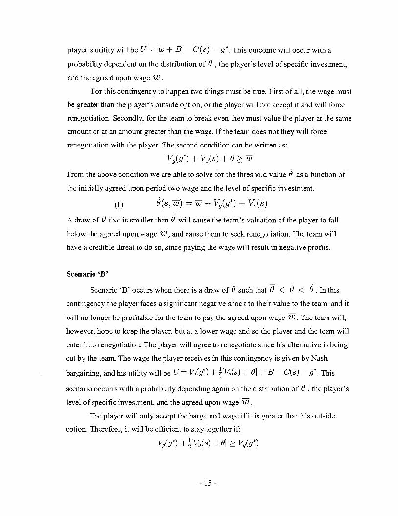
For this contingency to happen two things must be true. First of all, the: wage must

be greater than the player's outside option, or the player will not accept it and will force

renegotiation. Secondly, for the team to break even they must value the player at the same

amount or at an amount greater than the wage. If the team does not they will force

renegotiation with the player. The second condition can be written as:

Vg(g*) + Vs(s) + 8 2 5

From the above condition we are able to solve for the threshold value 8 as a function of

the initially agreed upon period two wage and th~e level of specific investment.

(1) B(s,m) = m - I$(g*) - Vs(s)

A draw of 8 that is smaller than 9 will cause the team's valuation of the player to fall

below the agreed upon wage z , and cause them to seek renegotiation. The team will

have a credible threat to do so, since paying the wage will result in negative profits.

Scenario 'B'

Scenario 'B' occurs when there is a draw of 8 such that $ < 8 < 8. In this

contingency the player faces a significant negative shock to their value to the team, and it

will no longer be profitable for the team to pay t:he agreed upon wage z . The team will,

however, hope to keep the player, but at a lower wage and so the player and the team will

enter into renegotiation. The player will agree to renegotiate since his alternative is being

cut by the team. The wage the player receives in this contingency is given by Nash

bargaining, and his utility will be U = Kh*) f i [ ~ ( s ) + 61 + B - C(s) - g". This

scenario occurrs with a probability depending again on the distribution of 8 , tlhe player's

level of specific investment, and the agreed upon wage G.

The player will only accept the bargained wage if it is greater than his outside

option. Therefore, it will be efficient to stay toge:ther if:

Vg(g*) + $!s(s) + 61 2 Vg(g*)

This condition allows us to solve for the threshold value of as a function of the players

specific investment. Simplifying the above condlition gives us: -

(2) Q) = - K(s) As long as the return from a specific investment is greater than the negative shock it will

remain efficient for the player to stay with the team.

Scenario 'C'

Scenario 'C' occurs when there is a draw of 8 which is less than 8, as defined

above. In this contingency there does not exist a Nash bargaining outcome for which the

player will agree to stay with the team. Instead they will leave the team to take their

outside option. The outside option could be a place on a roster with a different NFL team,

it could be a position on a CFL team, or might be the player's best option outside of

football. In this scenario the players utility will be U = &(g*) + B - g* - C(s). This

scenario occurs with a probability depending on the distribution of 8 and the player's

specific investment level.

A team and a player may initially agree upon a second period wage that is less than

the player's outside option, Vg(g*). In this case Nash bargaining will occur at t=2 as if

there were no contract in the first place. Given a draw of 6' that makes it efficient for the

parties to stay together (that is a draw where e > 77) the parties will negotiate a spot

contract according to Nash bargaining. Without an initial contract ?iJ > Vg(g') there

will be no 8^ threshold, and thus no scenario A.

One can see that investment in team specific skills will have two different effects on

the player's utility. The first, and obvious affect -is that greater investment will :increase a

team's valuation of a player, leading to a higher INash bargaining outcome in scenario B.

The second effect, which can be seen from equations (1) and (2), is that a greater

investment in specific skills will lower the thresh~old values of 6' , making it more likely

that the player will receive the contracted wage, a, and also more likely that he will stay

with the his current team.

Solving the Model for First Best Investment Levels

Efficiency requires two things. Ex-post efficiency is satisfied if a trading

relationship occurs whenever it is in the interests of both parties to do so. For this model

ex-post efficiency requires that if 8 is greater than 8 , the player and the team will agree

to stay together at t=2. Ex-post efficiency will allways be achieved.

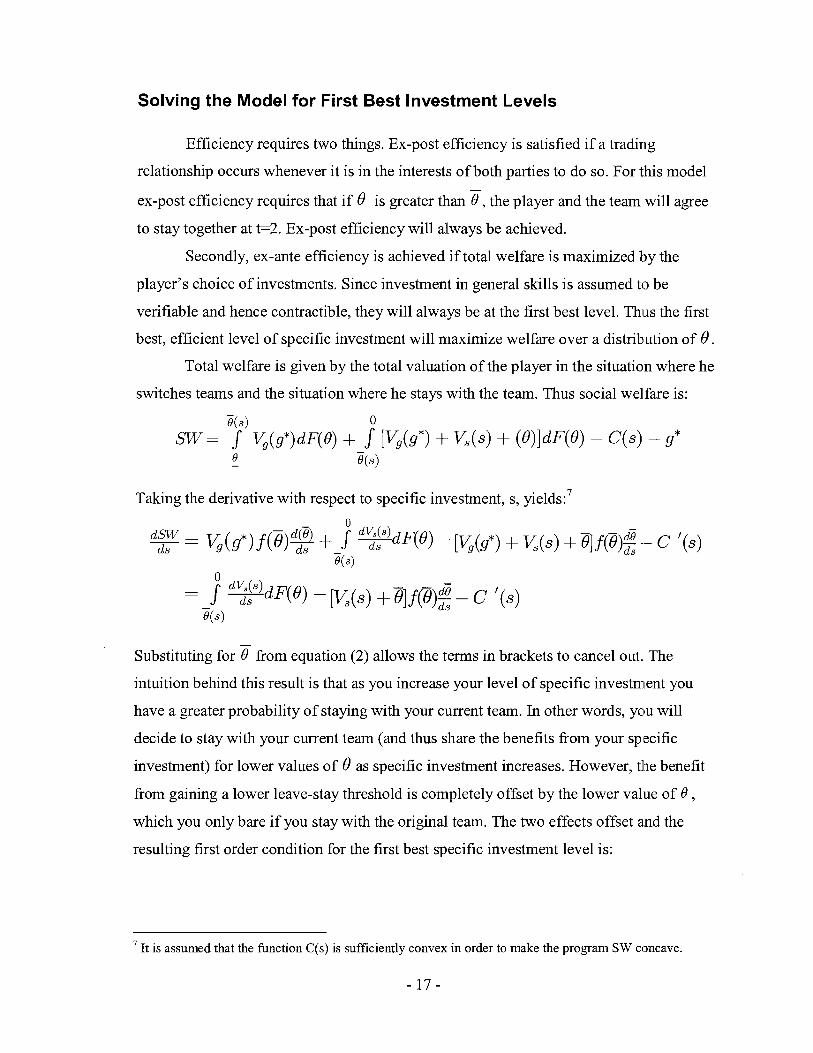
Secondly, ex-ante efficiency is achieved if total welfare is maximized by the

player's choice of investments. Since investment in general skills is assumed to be

verifiable and hence contractible, they will always be at the first best level. Thius the first

best, efficient level of specific investment will maximize welfare over a distriblution of 8 .

Total welfare is given by the total valuation of the player in the situation where he

switches teams and the situation where he stays with the team. Thus social welfare is:

Taking the derivative with respect to specific investment, s, yield^:^

0 dVs(s )

-- = - J F ~ ~ ( ~ ) - [v,(s) +8] f(B)g!- d s C '(s)

e ( s )

Substituting for 8 from equation (2) allows the terms in brackets to cancel out. The

intuition behind this result is that as you increase your level of specific investment you

have a greater probability of staying with your current team. In other words, you will

decide to stay with your current team (and thus share the benefits from your specific

investment) for lower values of 8 as specific investment increases. However, the benefit

from gaining a lower leave-stay threshold is com~pletely offset by the lower value of 8 ,

which you only bare if you stay with the original team. The two effects offset and the

resulting first order condition for the first best specific investment level is:

7 It is assumed that the function C(s) is sufficiently convex in order to make the program SW concave.

0

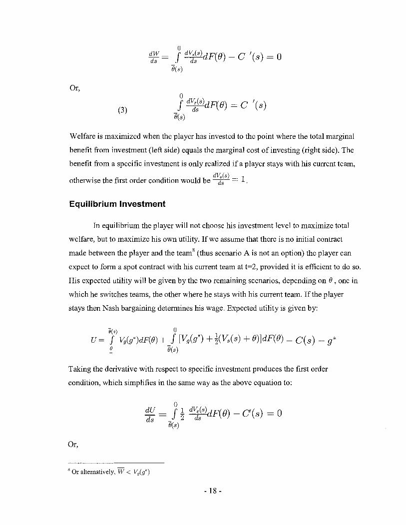
J m d ~ ( 0 ) d.9 = C ' ( s )

Welfare is maximized when the player has invested to the point where the total marginal

benefit from investment (left side) equals the marginal cost of investing (right side). The

benefit from a specific investment is only realized if a player stays with his cw~ent team,

d V , ( s ) otherwise the first order condition would be T~- = 1.

Equilibrium Investment

In equilibrium the player will not choose his investment level to maximize total

welfare, but to maximize his own utility. If we assume that there is no initial contract

made between the player and the team8 (thus scenario A is not an option) the player can

expect to form a spot contract with his current team at t=2, provided it is efficient to do so.

His expected utility will be given by the two remaining scenarios, depending on 8 , one in

which he switches teams, the other where he s t ~ y s with his current team. If the player

stays then Nash bargaining determines his wage. Expected utility is given by:

Taking the derivative with respect to specific investment produces the first order

condition, which simplifies in the same way as the above equation to:

8 Or alternatively, W < V,(g*)

When one compares equation (4) to equation (3), the impact of specific

investment becomes evident. With no initial contract, the team and the players will form a

spot contract so long as V,(S) > - 0, and thus achieve ex-post efficiency. The player will,

however, only receive half of the benefit from slpecific investments, and so he will under

dVs ( s ) invest in team specific skills. Because K ( s ) is concave in s, a higher value for d,

translates into a lower value of specific investment. Thus, without an initial contract the

player will expect to earn only a portion of his return from specific investments. The

intuition is that since the player knows he will be held up at t=2, he will under invest in

team specific skills.

Equilibrium Investment with an Initial Contract

If we allow for an initial contract of Z players will, with their choice of specific

investment, maximize their expected utility, as before. Now, however, expected utility is

given by:

The player's expected utility is comprised of outcomes A, B, and C as discussed

earlier. Which outcome the player actually finds himself in depends on his specific

investment level, the size of the contracted wage: i7, and of course, the draw of 8 . Taking the derivative with respect to specific investment produces:

This simplifies to:

Substituting from equation (1)

and

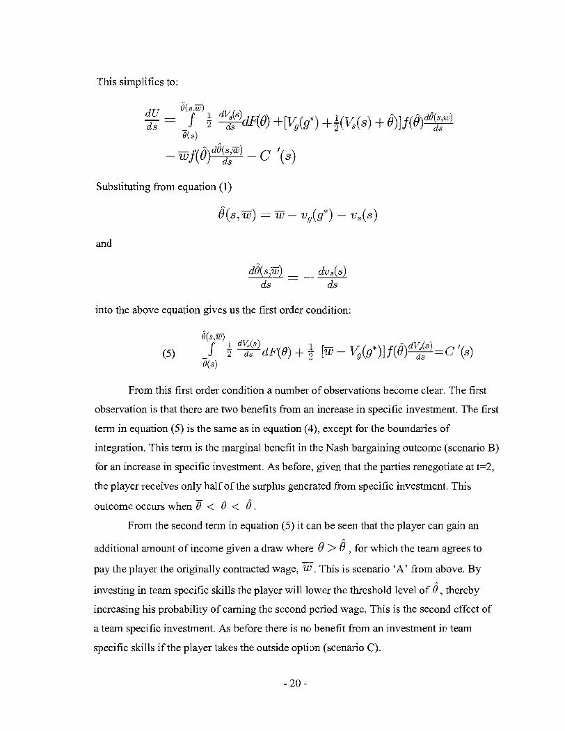
into the above equation gives us the first order condition:

From this first order condition a number of observations become clear. The first

observation is that there are two benefits from an increase in specific investment. The first

tern in equation (5) is the same as in equation (4), except for the boundaries of

integration. This tern is the marginal benefit in the Nash bargaining outcome (scenario B)

for an increase in specific investment. As before, given that the parties renegotiate at t=2,

the player receives only half of the surplus generated from specific investment. This

outcome occurs when < 6 < 8. From the second tern in equation (5) it c.an be seen that the player can gain an

A

additional amount of income given a draw where 6' > 6' , for which the team agrees to

pay the player the originally contracted wage, ui. This is scenario 'A' from above. By

investing in team specific skills the player will lower the threshold level of 8 , -thereby

increasing his probability of earning the second -period wage. This is the second effect of

a team specific investment. As before there is no benefit from an investment in. team

specific skills if the player takes the outside optison (scenario C).

The second observation is that even thou~gh the player may earn a greater return

from his specific investment if the team and the player are able to agree on an initial

contract, he will receive the full return from his specific investment in period two with a

probability of zero. This can be seen from the team's profit condition. If the player and

the team initially agree to a period two contract 20, the player knows he will only receive

the wage if Vg(g*) + Vs(s) + 6 > 5. Since investments in general skills will1 always be

the first best level, 20 implies a level of specific investments which the player must

perform in order to meet the team's profit condition. Because 8 equals zero with zero

probability and is by definition always non-positive, the player must invest beyond the

level implied by 20 if he wants to have some probability of earning the contracted wage.

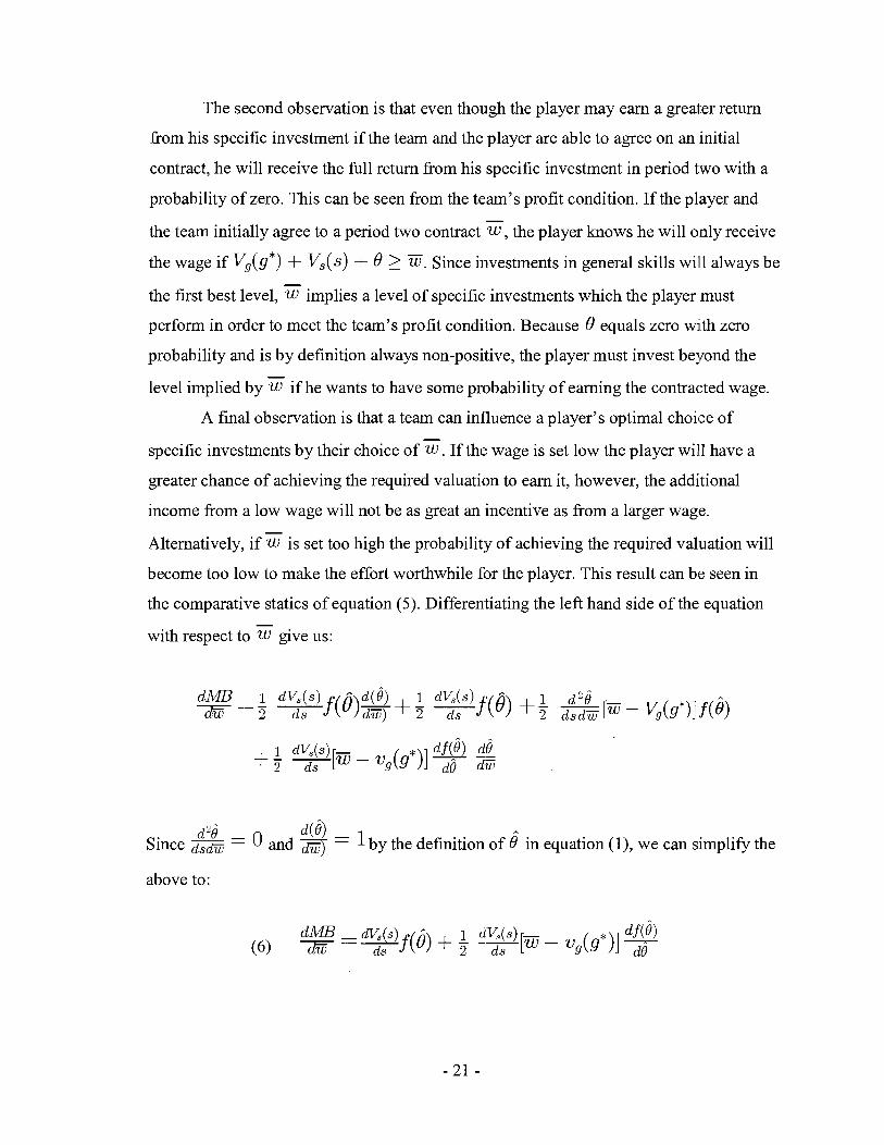
A final observation is that a team can influence a player's optimal choice of

specific investments by their choice of w. If the wage is set low the player will have a

greater chance of achieving the required valuation to earn it, however, the additional

income from a low wage will not be as great an incentive as from a larger wage.

Alternatively, if 20 is set too high the probability of achieving the required valuation will

become too low to make the effort worthwhile fix the player. This result can be seen in

the comparative statics of equation (5). Differentiating the left hand side of the equation

with respect to give us:

d% - 0 4) Since - and = 1 by the definition of 8^ in equation (I), we can simplify the

above to:

Equation (6) shows the change in the player's marginal benefit, for a level of

specific investment, given a change in the initia.lly contracted wage z. In other words, if

equation (6) is positive an increase in the wage will provide the player with a positive

incentive to increase his investment in specific skills. If equation (6) is negative an

increase in the wage will lead the player to want to reduce his investment in specific skills.

Determining the sign of equation (6) is easily done.

One can see that sign of the first term in the equation will always be po'sitive, by

the assumptions about the return to a specific investment. The sign of the second term

d f (6) depends on 7, which may be positive or negative depending on the distribution of

9 and the value of 8^. If we assume that the distribution of 6' is given by the normal

d f (@ ,. distribution, the sign of 7 will depend on the particular value of 0 . Therefore,

,. equation (6) will be positive over a range where 0 is relatively low, and turn negative

,.

over the range where 0 is relatively large. In this case we would expect to see a wage that

leads to a 8̂ in the interior of the distribution of 6' , and therefore z would be paid with

some positive probability.

Predictions

The first implication of the model is that an NFL player will always receive their

full return from investments in general skills. The player will not, however, be paid the

full value from their investment in specific skills. If there is no initial contract, the player

and the team will agree to a spot contract at t=2, so long as Nash Bargaining leads to a

wage that is greater than the player's outside option. The bargained wage will, however,

only pay the player a fraction of the value of his specific investment. Since the player will

expect to be held up he will under invest in specific capital.

Secondly, the model predicts that players and teams can do better with im initial

contract for the period two wage. By choosing the wage to maximize the player's

incentives, the team can induce a level of specific investment that is greater than had there

been no initial contract. Because the player still expects to be held up in period two he

will only agree to this second period wage if the surplus from the agreement is transferred

to him. This transfer is accomplished though the first period wage, B. Even though the

player is now obtaining a lump sum transfer, as well as a fixed wage with positive

probability, the player will still find it optimal to invest into the team's valuation. Thus,

the model predicts that a player in a position with a high degree of specific investment

will have a contract that covers both periods one and two, and which pays a greater first

period wage and a smaller second period wage than a similar player with low llevel of

team specific investments.

Finally, the model predicts that players in positions requiring a high degree of

specific investments will switch teams less often than those who play in positions that

mostly require investments in more general skillls. This is because players with more

specific skills can only capture some of the retmns fiom their specific investments if they

stay with the same team, while players with more general skills will be rewarded for their

investments by any team.

Testing the Predictions of the Model

Given the preceding predictions we would expect to see wages diminishing with

time for those positions that require team specifilc investments. The player with specific

skills would make a larger first period wage on account of the transfer, and subsequently

earn less as a result of hold-up. There are, however, several other factors that vvill

combine to increase salaries as players get older. One is that the players' investments in

themselves will continue each year. The return fi-om physical conditioning may reach a

plateau or a peak, but investments in learning arle likely to continue to add value to the

player throughout their career, even though at a diminishing rate. They will also become

better players with more game experience. These two effects will have an impact on a

player's performance statistics, but it will also increase the player's intangible qualities,

such as leadership ability, which will have an impact on the team's valuation olf the player,

but will not be evident from individual statistics. An additional effect is the NFL7s

bargaining agreement which has set a minimum wage for players that increases with the

player's experience level. It is therefore not surprising that Leeds & Kowalewski find

experience to have a significant positive (though diminishing) affect on a player's salary,

even when controlling for performance statistics.

Nonetheless, when performance variables and personal characteristics are

accounted for, the model predicts that players whose positions have a high degree of team

specificity will have larger initial wages than those who play positions with more

transferable skills, however, they will also find their salaries increasing at a lovver rate.

This is the main testable implication from the model.

An additional prediction is that players7 are less likely to switch teams jf their

position has a high degree of team specificity. This implication is owing to the fact that

players are still likely to receive a portion of the surplus, despite being held up, which

may give them a greater salary if they stay with the same team.

Description of the Data

The Dependent Variable

The dependent variable in the regression analysis is the amount of a player's

salary for a given year that is counted against thle salary cap. The Cap value includes the

current year's base salary and bonus pay, plus the signing bonus prorated over the full

period of the contract. Signing bonuses are the primary way for a team to creale flexibility

under the salary cap. By paying a player a signing bonus they can postpone much of the

cap value of the contract until future seasons, which allows teams to have a higher pay-

roll in a year they believe they are contenders. The salary cap value has been discounted

to 2000 dollars using the average of monthly CP'I values for the months of the NFL

season, which span more than one calendar year. The regression uses the natural

logarithm of the cap value to compress large values and to aid in the interpretation of the

coefficients.

The sample includes all players at the positions of interest who have significant

enough performance statistics to indicate regular play, and who had a minimurn of three

years of statistics available. Data for Salaries spans the years 2000 to 2004, while

personal statistics span the years 1999 to 2004. Any year in which a player switched

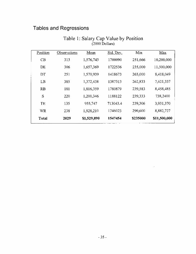
teams is excluded from the sample. Data for players' salaries comes from the USA

TODAY NFL Salaries ~ a t a b a s e s ~ . A summary of Salary statistics by position is found in

Table One.

The Independent Variables

There are a number of independent variables employed to control for variations in

a player's salary due to other factors than specificity. These include experience, a player's

height and weight, the year's salary cap figure and a range of performance statistics. It

was found that using multiple offensive statistics led to multicollinearity, and caused none

of the offensive statistics to be significant. When only yards were used the significance

level increased considerably. I believe yards provide as reasonable a measure of an

offensive player's productivity as can be gained from any statistic.

On the defensive side, however, there arle a number of significant perfc~rmance

measures. I believe this reflects the greater diversity of objectives among the d.efensive

positions chosen. All performance statistics and personal characteristics come from

N F ~ . c o m ' ~ . Players' statistics were used as averages per game and were lagged by one

period. Height and Weight are measured as the difference a player is from his positional

mean value. A summary of player statistics can be found in table two.

Specificity

The variable to capture specificity is a binary variable which indicates if the

player's position has a high degree of team specificity or a low degree of team specificity.

This variable is, admittedly, a potentially weak link in the data analysis. That some

positions demand high degrees of team specific investments while others do not seems

unquestionable. The quarterback is the prime example of a position that requirces a large

degree of learning in a team specific system. It is by far and away the most mentally

demanding position on the football field1'. On the other hand, a place kicker's skills are

probably perfectly transferable from team to tean-they just have to kick a ball through

some posts, and neither the ball nor the measurements of the posts change from team to

team. But while these positions typify the differences in specificity, they are not

comparable in a regression: the quarterback because it is a unique position in the NFL and

because they are paid for a number of intangible qualities; the kicker because their

personal statistics are not comparable to any othler position on the field. What we are left

with is a number of similar positions to compare. This similarity makes comparison

possible, but it also leads to more difficulty in classifying each position as specific or non-

specific. With this in mind, the specific and non-specific positions are as follows.

1 1 For this reason it was long believed that a black QB could not have success in the NFL. Though this prejudice has been proven false by many successful black QB's the informal segregation still exists at the coaching position, and strangely enough at Center, where there are currently no starting black ;athletes. The Center is the most mentally demanding position on the Offensive line.

Specific Non-Specific I Running Back 1 Safety I Wide Receiver

Defensive Tackle Linebacker

Tight End Cornerback

Defensive End

This classification was made based on my own intuition as well as the input from

an NFL sports col~rnnist '~. The distinction is motivated by the amount of specific

learning required for a given position, as well as by the amount of transferable skills in

that position.

For instance, a cornerback plays within a complex defensive system which is

designed to be hard to understand from the perspective of the opposing offense. This

complexity would give the comer high specificily; however, if we consider the profile of

a good comer we get a somewhat different picture. The best cornerbacks are valued for

their ability to play man-to-man coverage on a top receiver without any help 01- double

coverage. Furthermore, the cornerbacks are frequently the fastest and quickest players on

the field, qualities that are both highly coveted by teams, and perfectly transferable. For

these reasons I believe the cornerback position should be considered to have low team

specificity. In the preceding model the relative silze of the specific investment is

irrelevant--only the absolute size should matter. It is, however, not difficult to construct a

situation where the negative shock influences the valuation such that the relative size is

important.

There is a similar story with the defensive line positions. The defensive ends are

not all that different from the tackle position, and both require a large amount of learning

to play in a team's defense. The key difference between the positions is that ends are

valued for their ability to rush the quarterback much more than tackles are. It is the ability

of the defensive end to physically beat the player lined up opposite him which makes the

player an effective one, and this skill seems to rely more on individual ability than on a

team system. For this reason I consider the defensive ends to be non-specific positions

and yackles to be specific. In both these cases one can see how a comer and an end

12 Jeff Legwold writes for the Rocky Mountain News, out of Denver.

should be able to switch teams and have an instant impact in the team's defensive system,

while it will be more difficult for specific positions to have a similar effect.

I have classified the safeties as non-specific, consistent with Jeff Legwold. Their

responsibilities are mostly in deep coverage with occasional blitzing. On the other hand

the linebackers play a much more diverse role in the defense. This is particularly true

when you consider the different formations that teams use for their linebackers.. The New

England Patriots won three Super Bowls using flour (and occasionally five) linebackers,

rather than a traditional formation with three. Since then many other teams have been

adopting this system, which demands more versatile play from the linebackers..

For the offensive positions I have mostly relied on Jeff Legwold's insight. Most

tight ends are not used as extensively in the passing game, and their routes do not depend

as much on timing or precision. Tight ends are valued for their ability to block larger

opposing players, which depends on size and strength, abilities that are perfectly

transferable. In contrast, wide receivers must be more precise in their routes, which

depends heavily on learning the particular offensive system and also on gaining a

familiarity between the receiver and the quarterbsack. Access to a teammate car1 cause as

much of the specificity problem as access to a te.am's systems.

A further complication is that the value of a player will depreciate differently

depending on the position he plays. Running backs, for example, are subjected to an

incredible amount of pounding, and so their value to the team depreciates much faster

than players at other positions. While it is not possible to control for different r.ates of

depreciation between positions, there is enough variation in depreciation rates among the

pools of specific and non-specific positions that iit should not influence the resu-lts.

Old Dummy

The Dummy Variable "OLD" is defined as a player who is in their third year or

greater. The third year is the earliest year that a player may be considered a free agent

once their contract expires. It is used as an interaction term with the specific dummy to

capture the effect of a player's specificity on salary over time. Specificity is also

interacted with experience to test the robustness of the results.

Estimation and Results

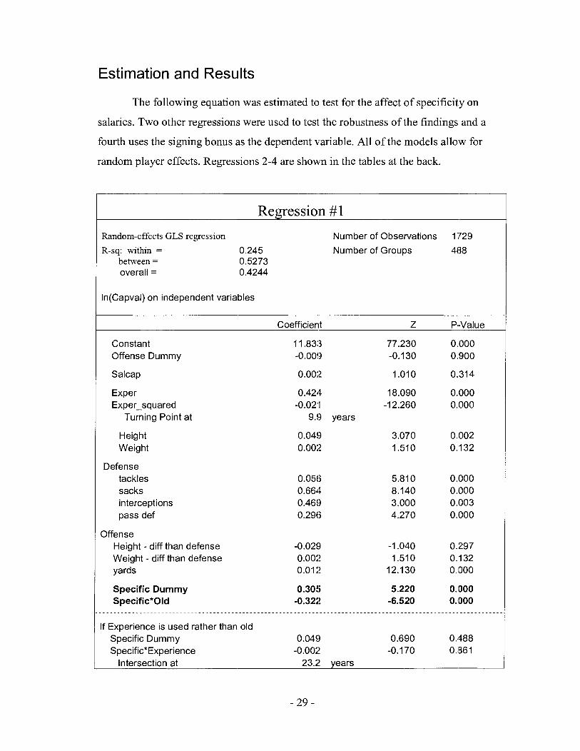
The following equation was estimated to test for the affect of specificity on

salaries. Two other regressions were used to test the robustness of the findings and a

fourth uses the signing bonus as the dependent variable. All of the models allow for

random player effects. Regressions 2-4 are shown in the tables at the back.

Regression # 1

Random-effects GLS regression Number of Observations 1 ;729

R-sq: within = 0.245 Number of Groups 488 between = 0.5273 overall = 0.4244

In(Capva1) on independent variables

Coefficient Z P-Value

Constant Offense Dummy

Salcap

Exper Exper-squared

Turning Point at

Height Weight

Defense tackles sacks interceptions pass def

Offense Height - diff than defense Weight - diff than defense yards

Specific Dummy Specific*Old

If Experience is used rather than old Specific Dummy Specific*Experience

Intersection at 23.2 years

- 29 -

The coefficients on the specific dummy ;md the specific interaction term are both

statistically significant and have the predicted signs. The analysis suggests thal; players in

specific skill positions make 0.30 log points, or approximately 30% more than others in

their first years of playing, after which they can expect to be paid 0.32 log points less-

approximately 32% less each year. For the average salary in our sample this difference

amounts to about $450,000. It should also be remembered that this sample excludes the

quarterback position, the highest paid and most team specific of all the positions.

This result is also robust to changes in the specification. Regression Two allows

for variations in the intercepts based on positions, rather than using the specific dummy

variable. The result shows a similar value for the specific interaction term-negative 0.3

log points and statistically significant. It also shows larger intercepts for each of the

positions that have been classified as team specific. Comparing the results in R-egression

Two to the table of average salaries reveals that it is not simply the higher mean salaries

that drive the difference in the intercepts. The defensive tackle and the linebackers both

have higher intercepts than the cornerbacks desplite having lower average salaries.

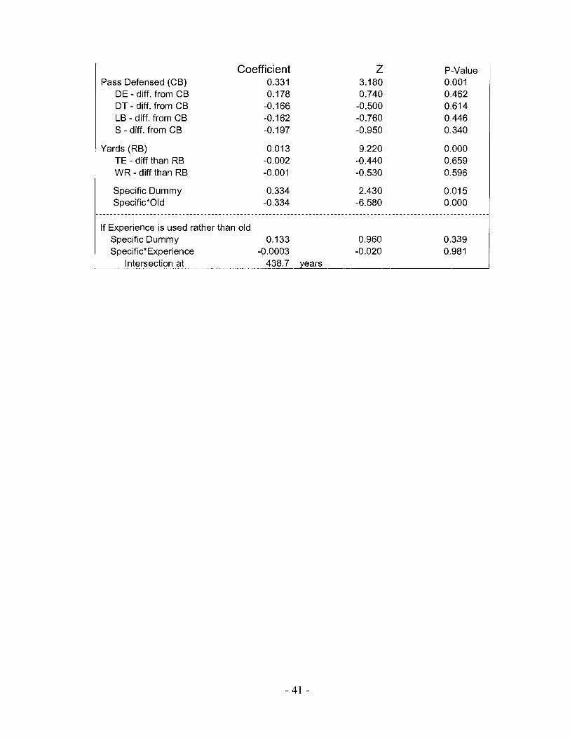
Regression Three allows the performance statistics to be interacted with the

positional dummy variables. The results of this regression are as expected, with

perfonnance measures becoming more significant the closer they mirror the position's

main responsibilities. For instance the cornerback has a much larger and more significant

coefficient on passes defensed than the other positions, but actually has a negative

coefficient on sacks13. The coefficients for the specific dummy and the specific:

interaction term do not change meaningfully with the additional variables.

Unfortunately, the results are not robust to changes in the definition of the old

dummy variable. If old is defined as a player who is in their fourth season or more, than

the coefficients lose significance. If specificity is interacted with experience rather than

with the dummy variable old the significance of the coefficients are lost, though the signs

remain as expected. Each regression reported lists the coefficient for specificity interacted

with experience in the alternative specification.

13 It is not entirely surprising that salary would be inversely related to sacks for CBs. If you were going to blitz with one of your Comers and leave the other in coverage I would be inclined to blitz with the one who is least effective in coverage.

Regression Four replaces the salary cap value with the signing bonus as the

dependent variable. The results show that signing bonuses do not appear to be determined

by the amount of team specificity. It is likely that there are too many other factors

involved in determining the structure of the salary, foremost of which is probably the

desire of teams to have flexibility with their cap. A further consideration might be the

durability of the player, considering that signing bonuses must be paid if the even if the

player fails to make the team the next season. If the player is no longer part of the team

the signing bonus must be paid off in an accelerated way, giving teams additional cap

problems which they would not have anticipated. The result is that teams will avoid

paying signing bonuses unless they are sure of a long term relationship with the player. It

is not necessary for our results that highly specific positions receive the signing bonus

more than others since the transfer at period one can be in terms of the base salary just as

easily.

Several other interesting observations can be seen from the estimation. A player's

weight is insignificant or marginally positive, contrary to expectations that it would have

a large influence. A possible explanation is that the variable for weight is capturing the

affects of the omitted variable speed. If speed could be included in the regressi'on than I

would expect both it and weight to be positive and significant. However, since speed

cannot be controlled for, and since it is likely very negatively correlated to weight, the

results for a player's weight captures much of this additional affect.

Testing for Mobility

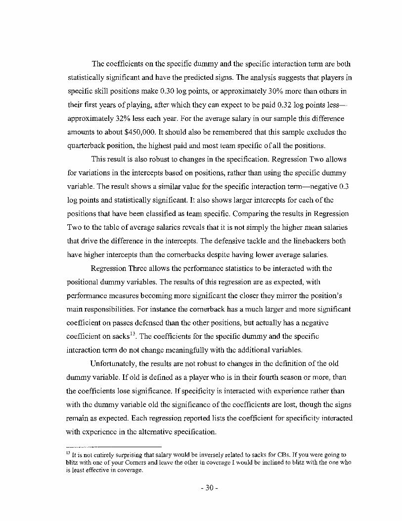
If we examine the number of players who have switched teams at least once

during our sample it shows that players who are considered to have more specific skills

will switch teams less often. These results are not particularly strong, however, since we

cannot reject the null hypothesis that specific pla.yers switch teams more often.

Team Switchers by Specific and -----I Non-Specific Positions phcd n M Perrent

Non-Specific 140 98 238 41 %

Specific 1 54 9Q 244 36%

Total 2 94 188 482 39%

P-value for Ho: Mean < Mean specific = 0.1 677

Also worth noting is that the most frequent team switchers are the cornerbacks

and the safeties. One would expect the frequency of switching teams to increase with

playing experience, and these two positions tend to have long playing careers. Table Six

has a complete list of team switchers by position as well as the average experience by

position. What we find is that the specific positions tend to have longer careers than the

non-specific positions, and so this explanation can be ruled out.

To control more formally for the affect olf experience and skill level on a player's

decision to switch teams I estimate a Probit regression, where the dependent variable is a

binary variable indicating whether the player has switched teams or not in the :sample. A

team switcher is given by a value of one. The reisults are as follows.

Probit Regression

Probit Estimate Observations 467

LR c h i 9 (8) 145.67

Log likelihood =-237.54522 Prob > chiA2 0

Pscsudo RA2 0.2347

Switcher on independent variables

Offense yards

Specific Dummy -0.191 -0.070 -1 . I 80 0.237

Mlarginal Effects Coefficient (valued at the mean) z P-Value

Constant -3.359 -7.960 0.000

Exper 0.909 0.333 7.240 0.000 Exper-squared -0.044 -0.01 6 -5.340 0.000

defense tackles -0.030 -0.01 1 -0.750 0.456 sacks -0.986 -0.360 -2.560 0.01 0 interceptions -0.668 -0.244 -0.770 0.441 pass def -0.649 -0.237 -1.590 0.113

As was expected, experience is strongly correlated to the probability of'a player

switching teams. I also find that performance levels are negatively correlated to the

probability of a player switching teams, so that better players do not switch teams as

frequently. Finally, players in specific positions are approximately 7% less likely to

switch teams in their career. Although the result:; are not particularly significant, the

negative coefficient on specificity is robust to ch.anges in the model's specifications.

Conclusions

This paper has argued that positions in the NFL vary by the degree of team

specific investment that they are required to make. From a theoretical perspective we can

expect this specificity to lead to longer contracts for these positions and for the salary to

be disproportionately loaded onto the first years of the contract. An examination of the

data supports the predictions of the model. Players in specific skill positions begin with a

higher initial wage, but find that their wages increase at a lower rate over time, when all

else is held constant. I also find some evidence to support the prediction that players who

make specific investments will switch teams less often.

Tables and Regressions

Table 1 : Salary Cap Value by Position (2000 Dollars)

Position Observations Mean Std. Dev. &

CB 313 1,576,743 1700090 25 1,666

DE 3 06 1,657,369 1722536 235,000

DT 25 1 1,570,939 1418673 265,000

LB 385 1,372,438 1387313 262,833

RE3 181 1,816,359 1780879 239,583

S 220 1,200,346 1188122 239,333

TE 135 955,747 713043.4 239,306

WR 23 8 1,928,210 1746023 290,600

Total 2029 $1,529,890 1547454 $235000

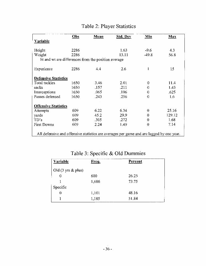
Table 2: Player Statistics

Obs - Mean Std. Dev Min Max Variable

Height 2286 1.63 -9.6 4.3 Weight 2286 13.11 -49.8 56.8

ht and wt are differences from the position average

Experience 2286 4.4 2.6 1 15

Defensive Statistics Total tackles 1650 3.46 2.01 0 11.4 sacks 1650 .I57 .2 1 1 0 1.43 Interceptions 1650 .065 . 106 0 .625 Passes defensed 1650 .243 .256 0 1.6

Offensive Statistics Attempts 609 6.22 6.34 0 25.16 yards 609 45.2 29.9 0 129.12 TD's 609 .3085 .272 0 1.68 First Downs 609 2.24 1.49 0 7.14

All defensive and offensive statistics are averages per game and are lagged by one year.

Table 3: Specific & Old Dummies Variable Freq. Percent

Old (3 yrs & plus) 0 600 26.25 1 1,686 73.75

Specific 0 1,101 48.16 1 1,185 51.84

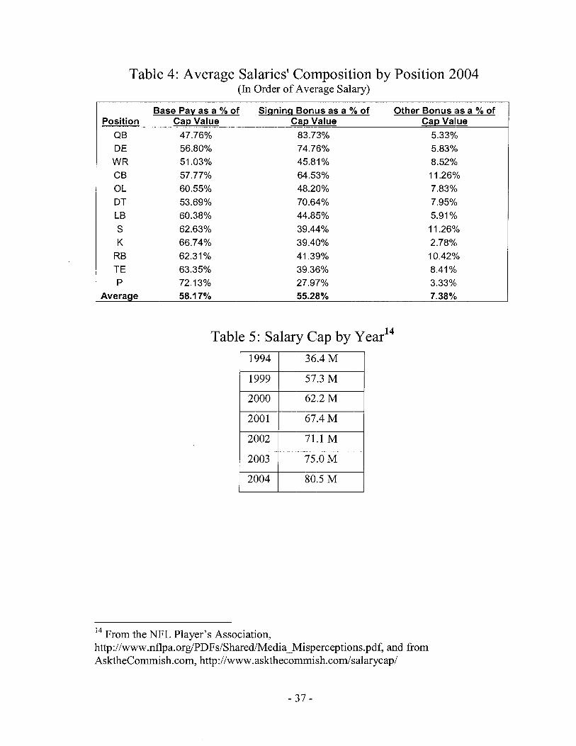
Table 4: Average Salaries' Composition by Position 2004 (In Order of Average Salary)

Base Pav as a % of Sinnincr Bonus as a % of Other Bonus ins a % of Position Cap Value Cap Value Cap Value

QB 47.76% 83.73% 5.33%) DE 56.80% 74.726% 5.83%) W R 51.03% 45.81 % 8.52%) CB 57.77% 64.5,3% 11.26% OL 60.55% 48.210% 7.83%) DT 53.69% 70.64% 7.95%1 LB 60.38% 44.8:5% 5.91 %I S 62.63% 39.44% 11.26% K 66.74% 39.40% 2.78%) RB 62.31 % 41.3!3% 10.4296 TE 63.35% 39.36% 8.41 %I

P 72.13% 27.9'7% 3.33%) I Average 58.1 7% 55.28% 7.38% 1

Table 5: Salary Cap by year14

14 From the NFL Player's Association, http://www.nflpa.org/PDFs/Shared/Media-Misp~erceptions.pdf, and from AsktheCommish.com, http://www.askthecommi~~h.com/salarycap/

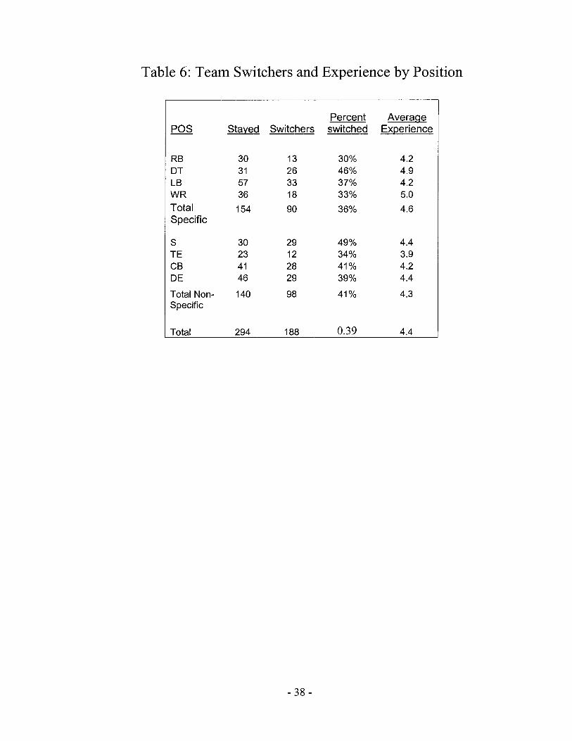
Table 6: Team Switchers and Experience by Position

Percent Average poS Stayed Switchers switched Experience

RB 30 13 30% 4.2 DT 3 1 26 46% 4.9 LB 57 33 37% 4.2 WR 36 18 33% 5.0 Total 1 54 90 36% 4.6 Specific

Total Non- 140 98 41 % 4.3 Specific

Total 294 188 0.39 4.4

Regression #2

Random-effects GLS regression Num. of Observations

R-sq: within = 0.4283 Num. of Groups

between =

overall =

In(Capva1) on independent variables

Constant

Salcap

Experience Experience-squared

Turning Point at

Height Weight

Defense tackles sacks interceptions pass def

Offense Height - diff from defense Weight - diff from defense yards

Position Dummies CB DE DT* LB* RB* S TE WR*

Coefficient

11.799

0.003

0.41 6 -0.02!1

9.9 years

0.0417 0.003

dropped 0.07'0 0.44 1 0.2013 0.2687

-0.173 0.03 1 0.31 0

-0.336

Experience used rather than old (Note: other coefficients change but are not reported) Specific*Experience -0.006 -0.460 0.647

* indicates specific positions.

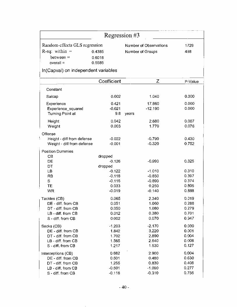
Random-effects GLS regression Number of Observations 1 '729

R-sq: within = 0.4385 Nu~mber of Groups 4i38

between = 0.601 8 overall = 0.5585

In(Capva1) on independent variables

Regression #3

Coefficient Z P.-Value

Constant

Salcap

Experience Experience-squared Turning Point at

Height Weight

Offense Height - diff from defense Weight - diff from defense

Position Dummies CB DE DT LB RB S TE WR

Tackles (CB) DE - diff. from CB DT - diff. from CB LB - diff. from CB S - diff. from CB

Sacks (CB) DE - diff. from CB DT - diff. from CB LB - diff. from CB S - diff. from CB

Interceptions (CB) DE - diff. from CB DT - diff. from CB LB - diff. from CB S - diff. from CB

0.421 -0.021

9.8 years

dropped -0.1 26

dropped -0.122 -0.1 I8 -0.1 I6 0.033

-0.01 9

Coefficient Pass Defensed (CB) 0.331

DE - diff. from CB 0.178 DT - diff. from CB -0.1 66 LB - diff. from CB -0.1 62 S - diff. from CB -0.197

Yards (RB) TE - diff than RB WR - diff than RB

Specific Dummy 0.334 2.430 0.01 5 Specific*Old -0.334 -6.580 0.000

- - - - - - - - - - - - - - - - - - - - - - - - - - - - - - - - - - - - - - - - - - - - - - - - - - - - - - - - - - - - . - - - - - - - - - - - - - - - - - - - - - - - - - - - - - - - - - - - - - - - - - - - - - - -

If Experience is used rather than old Specific Dummy 0.133 0.960 0.339 Specific*Experience -0.0003 -0.020 0.981

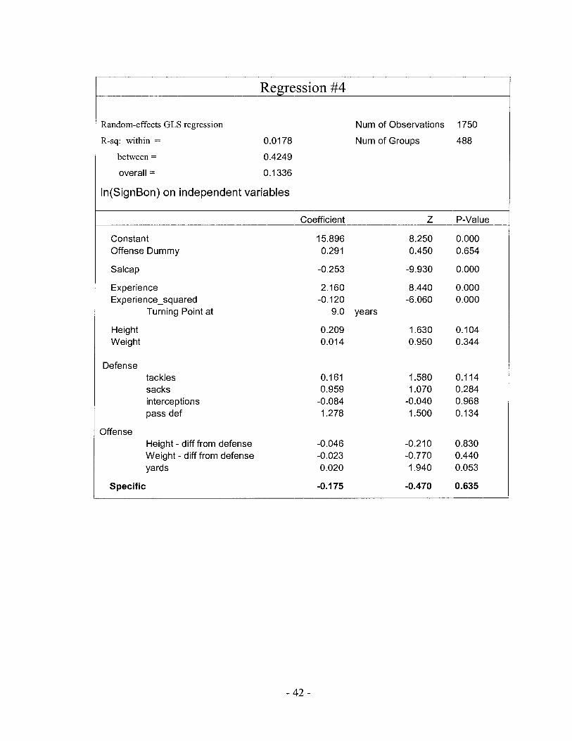
Regression #4

Random-effects GLS regression

R-sq: within = 0.01 78

between = 0.4249

overall = 0.1 336

In(SignBon) on independent variables

Num of Observations 1750

Num of Groups 488

Coefficient Z P-Value

Constant Offense Dummy

Salcap

Experience Experience-squared

Turning Point at

Height Weight

Defense tackles sacks interceptions pass def

Offense Height - diff from defense Weight - diff from defense yards

Specific

15.896 0.291

-0.253

2.160 -0.120

9.0 years

0.209 0.014

Ask the Commish, "Capenomics." AsktheComnnish.com http://www.askthecomrnish.com/salarycap/ (Accessed February, 2006).

Borghesi, Richard. "Allocation of Scarce Financial Resources: Insight from the NFL Salary Cap" (Draft: May, 2004). http://www.business.txstate.edu~users/rb3 8/NFL - Salary-Cap.pdf (Acc'essed January, 2006).

Conlin, Michael and Emerson, Patrick M. "Mul1:idimensional Separating Equilibria and Moral Hazard: An empirical study of National Football League Contract Negotiations" in The Review of Economics and Statistics, August 2003, 85(3): 760-765.

Hart, Oliver (1995): Firms, Contracts and Financial Structure, Oxford, UK, Olxford University Press

Heubeck, Tina and Scheuer, Jochen. "Incentive Contracts in Team Sports - Theory and Practice (Draft)." http://eale2002.phs.uoa.gr/papers/Heubeck%2O&%2OScheuer.pdf (Accessed November 29,2005).

Krieger, Dave. "Can Plummer work without a safety net?" in The Rocky Mountain Navs. h t t p : / / w w w . r o c k y m o u n t a i n n e w s . c o m / d r r n n / s p o ~ i c l e / O , 1299,DR MN-83-4408 135,OO.html. (Accessed January 23,2006)

Leeds, Michael A. and Kowalewski, Sandra (2001): Winner Take All in the NFL: The Effect of the Salary Cap and Free Agency on the Compensation of Skill Position Players. Journal of Sports Economics 2:3.

Legwold, Jeff. "Broncos Inbox". The Rocky Mountain News. http:/lblogs.rockymountainnews.com/denver/broncos/

NFL.com, "NFL Stats Home," http://www.nfl.com/stats (Accessed January-February, 2006)

NFL Player's Association, "Misperceptions". wm.nflpa.org http://www.nflpa.org/PDFs/SharedlMedia - Misperceptions.pdf (Accessed February, 2006).

Prisco, Pete. CBS Sports, "CBSsportsline.com~' ~www.cbssportsline.com

Schmitz, Patrick W. (2001): The Hold-Up ProbLem and Incomplete Contracts: A Survey of Recent Topics in Contract Theory. Bulletin of Economic Research 53 : 1.

Sutton, John, "Non-Cooperative Bargaining Theory: An Introduction," in The Review of Economic Studies, Vol. 53, No. 5 (Oct. 1 986), 709-724.

USA Today, "NFL Salaries Database," h t t p : / / a s p . u s a t o d a y . c o m / s p o r t s / f o o t b a l ~ l t . a s p x (Accessed January

- February, 2006).

Weisstein, Eric W. "Leibniz Integral Rule." From Math World--A Wolfram Web Resource. h t t p : / /ma thwor ld .wo l f r am.con l /Le ibn i z In t e~ l (Accessed March 5,2006)

Wooldridge, Jeffrey M. Introductory Econometrics: A modern Approach. Tho:mson, South-Westem. 2003.