Hodge Dualities on Supermanifolds

L. Castellani a,b,∗, R. Catenacci a,c,†, and P.A. Grassi a,b,‡ .

(a) Dipartimento di Scienze e Innovazione Tecnologica, Universita del Piemonte Orientale

Viale T. Michel, 11, 15121 Alessandria, Italy

(b) INFN, Sezione di Torino, via P. Giuria 1, 10125 Torino

(c) Gruppo Nazionale di Fisica Matematica, INdAM, P.le Aldo Moro 5, 00185 Roma

Abstract

We discuss the cohomology of superforms and integral forms from a new perspective based

on a recently proposed Hodge dual operator. We show how the superspace constraints (a.k.a.

rheonomic parametrisation) are translated from the space of superforms Ω(p|0) to the space

of integral forms Ω(p|m) where 0 ≤ p ≤ n, n is the bosonic dimension of the supermanifold

and m its fermionic dimension. We dwell on the relation between supermanifolds with non-

trivial curvature and Ramond-Ramond fields, for which the Laplace-Beltrami differential,

constructed with our Hodge dual, is an essential ingredient. We discuss the definition of

Picture Lowering and Picture Raising Operators (acting on the space of superforms and on

the space of integral forms) and their relation with the cohomology. We construct non-

abelian curvatures for gauge connections in the space Ω(1|m) and finally discuss Hodge dual

fields within the present framework.

July 4, 2015

∗leonardo.castellani@mfn.unipmn.it†roberto.catenacci@mfn.unipmn.it‡pietro.grassi@mfn.unipmn.it

Contents

1 Introduction 2

2 Background Material 4

2.1 3d,N = 1 . . . . . . . . . . . . . . . . . . . . . . . . . . . . . . . . . . . . . . 4

2.2 (Super)Hodge dual . . . . . . . . . . . . . . . . . . . . . . . . . . . . . . . . . 6

2.3 Metric and Supergroups . . . . . . . . . . . . . . . . . . . . . . . . . . . . . . 14

3 Complex of Forms 16

3.1 Horizontal Differentials: d, d†,∆. . . . . . . . . . . . . . . . . . . . . . . . . . . 16

3.2 Vertical Differentials: Y,Z. . . . . . . . . . . . . . . . . . . . . . . . . . . . . 20

4 Constraints, Rheonomy and Cohomology 25

4.1 Non-abelian Gauge Fields . . . . . . . . . . . . . . . . . . . . . . . . . . . . . 28

5 Dualities 30

1

1 Introduction

Recently some issues regarding the structure and the properties of forms on supermanifolds

have been clarified. This has motivated the introduction of a new set of basic forms (called

integral forms) [1, 2] which can be integrated on supermanifolds and are useful for several

applications in string theory and quantum field theory [3, 4, 5, 6, 7, 8]. It has been shown also

how the usual manipulations derived from the Cartan calculus can be used. More recently,

in [9], a definition of Hodge dual has been proposed. It is based on the Fourier transform for

differential forms and is involutive. This new geometrical ingredient opens up the possibility

of studying some aspects of Hodge theory for differential forms on supermanifolds.

An important ingredient in the geometry of the supermanifolds is given by integral forms.

As discussed in [7, 8] they are essential for a theory of integration of forms on supermanifolds.

The wedge products of the differentials dθ (θ being the anticommuting coordinates) are com-

muting and therefore there is no canonical top form. To solve this problem, one introduces a

distribution-like quantity δ(dθ) for which a complete Cartan calculus can be developed. The

distributions δ(dθ) enter the definition of integral forms.

The next step, tackled in [9], is the construction of a Hodge dual operator ? for super-

manifolds, that allows to apply well-known techniques such as Hodge theory to study the

cohomology classes of a given (super)manifold. In particular, for a compact bosonic mani-

fold M endowed with a global metric g, one can introduce a nilpotent differential operator

d† = ?d? (also called codifferential; ? is the Hodge dual operator) and the Laplace-Beltrami

differential ∆ = d† d + d d†. The latter is used to compute harmonic forms (∆ω = 0) and

the Hodge theorem states that for each de Rham cohomology class on M , there is a unique

harmonic representative. Obviously, due to invertibility of ? for a given cohomology class of

d (de Rham cohomology) there exists a cohomology class of d†.

In the case of supermanifolds, the complex of pseudo-forms Ω(p|q) is filtered according to

two numbers: p, the form number and q the picture number. We have denoted by superforms

those with vanishing picture, Ω(p|0). They have no bound on the form degree. We have denoted

by integral forms the complex Ω(p|m), where m is the fermionic dimension of the supermanifold

2

and p ≤ n (with n the bosonic dimension). The d operator can be conveniently extended; it

increases the form number without touching the picture number. The Hodge dual operator

maps a superform to an integral form (and therefore the picture number is changed). In

particular, ? maps Ω(p|0) to Ω(n−p|m). Therefore, d† maps Ω(p|0) to Ω(p−1|0) and equivalently

maps Ω(p|m) to Ω(p−1|m). In terms of d†, we can finally define a Laplace-Beltrami differential.

In the present work, we study the codifferential d† and the Laplace-Beltrami differential

∆ on supermanifolds. Before doing that, we have to clarify what type of cohomology we are

describing. If we consider a flat supermanifold, applying the Poincare lemma (see for example

[6]) it turns out that all closed superforms with positive form degree are exact and therefore the

cohomology coincides with the constant (0|0)-forms. However, in the case of superforms, one

can impose some external auxiliary conditions (known as superspace constraints or rheonomic

conditions) which make the cohomology non-trivial. Let us consider an example: in three

bosonic and two fermionic dimensions the gauge field belongs to a supermultiplet made out

of a vector field (with 3 d.o.f.’s, modulo the gauge transformations) and a spinor field (with

2 d.o.f.’s) . They can be cast into a vector superfield Aa or into a spinor superfield Aα which

are the components of a 1-superform. Therefore, a 1-superform contains too much freedom

for describing a single gauge supermultiplet. By a clever choice of some constraints, one can

preserve the covariance with respect to supersymmetry transformations, reduce the number

of independent superfields and restrict the physical field content to the one of a single gauge

supermultiplet.

In addition, the computation of the cohomology with these external constraints (which can

be also be viewed as an equivariant cohomology) gives the irreducible representations of the

superspin([11]). Until now, the computation has been performed on the space of superforms

Ω(p|0), for which the form degree is not limited by the bosonic dimension of the supermanifold

(in the example, this is 3) and is in fact unbounded. Potentially, at any given form degree

we might have new cohomology classes and new multiplets. On the other side, we have seen

that there is a new complex of forms Ω(p|m) that, as we discuss in the following, is related

by Hodge duality to the complex of superforms Ω(p|0), and therefore we should be able to

relate the corresponding cohomology classes. In addition, for this new complex there is a

3

natural upper bound, but there is no lower bound. The complex of integral forms Ω(p|m) has

maximum p equal to the bosonic dimension and maximum m equal to fermionic dimension

of the supermanifold, but, on the other hand, it contains also negative degree forms (by

considering the derivatives of the Dirac delta forms). If there is a map of cohomology classes

between Ω(p|0) and Ω(p|m), it appears clear that the interesting cohomology classes must be

contained into the range of the non-trivial classes of both complexes.

In Sec. 2, some background material is given to set the stage and to fix the conventions

used in the rest of the paper. In Sec. 2.2, we discuss the (super)Hodge dual operator for

a generic metric on a given supermanifold. In Sec. 2.3, the relation between Hodge theory,

Laplace-Beltrami differential and the metric on supergroup manifolds is exploited. In Sec. 3

the complex of forms is studied and in Sec. 3.1, the horizontal differentials are constructed.

On the other hand, in Sec. 3.2 the vertical differentials are introduced and discussed. In Sec.

4, the relation between superspace constraints for superforms and superspace constraints for

integral forms is explored. In Sec. 4.1 non-abelian field strengths are constructed. Finally

Sec. 5 deals with dualities.

2 Background Material

2.1 3d,N = 1

We recall that in 3d N=1, the supermanifold M3|2 (homeomorphic to R3|2) is described

locally by the coordinates (xa, θα), and in terms of these coordinates, we have the following

two differential operators

Dα =∂

∂θα− 1

2(γaθ)α∂a , Qα =

∂

∂θα+

1

2(γaθ)α∂a , (2.1)

a.k.a. the superderivative and the supersymmetry generator, respectively. They have the

properties

Dα, Dβ = −γaαβ∂a , Qα, Qβ = γaαβ∂a , Dα, Qβ = 0 (2.2)

In 3d, we use real and symmetric Dirac matrices γmαβ. The conjugation matrix is εαβ and

a bi-spinor is decomposed as follows: Rαβ = Rεαβ + Raγaαβ , where R = −1

2εαβRαβ and

4

Ra = tr(γaR) are a scalar and a vector, respectively. In addition, it is easy to show that

γabαβ ≡ 12[γa, γb]αβ = iεabcγcαβ.

Given a (0|0)-form Φ(0|0), we can compute its supersymmetry variation (viewed as a super

translation) as a Lie derivative Lε with ε = εαQα + εa∂a (εa and εα are the infinitesimal

parameters of the translations in the x and θ coordinates, respectively) and we have

δεΦ(0|0) = LεΦ(0|0) = ιεdΦ(0|0) = ιε

(dxm∂mΦ(0|0) + dθα∂αΦ(0|0)

)= (2.3)

= (εm +1

2εγmθ)∂mΦ(0|0) + εα∂αΦ(0|0) = εm∂mΦ(0|0) + εαQαΦ(0|0)

In the same way, acting on (p|q) forms, where p is the form degree and q is the picture number,

we use the usual Cartan formula Lε = ιεd+ dιε.

To compute the differential of Φ(0|0), we can use a set of invariant (1|0)-forms

dΦ(0|0) = dxm∂mΦ(0|0) + dθα∂αΦ(0|0) = (2.4)

=(dxm +

1

2θγmdθ

)∂mΦ(0|0) + dθαDαΦ(0|0) ≡ Πm∂mΦ(0|0) + ΠαDαΦ(0|0)

with the property of being invariant under supersymmetry transformations, namely δεΠm =

δεΠα = 0.

The particular top form represented by the expression

ω(3|2) = εmnpΠm ∧ Πn ∧ Πp ∧ εαβδ(dθα) ∧ δ(dθβ) , (2.5)

has the properties:

dω(3|2) = 0 , Lεω(3|2) = 0 . (2.6)

It is important to point out the transformation properties of ω(3|2) under a Lorentz transforma-

tion of SO(2, 1). Considering Πa, which transforms in the vector representation of SO(2, 1),

the combination εmnpΠm∧Πn∧Πp is clearly invariant. On the other hand, dθα transform under

the spinorial representation of SO(2, 1), say Λ βα = (γab) β

α Λab with Λab ∈ so(2, 1), and thus

an expression like δ(dθα) is not covariant. Nonetheless, the combination εαβδ(dθα)δ(dθβ) =

2δ(dθ1)δ(dθ2) is invariant as can be proved using the properties of the δ-forms. In addition,

5

ω(3|2) has a bigger symmetry group: we can transform the variables (Πα, dθα) under an ele-

ment of the supergroup SL(3|2). Note that ω(3|2) is a section of the Berezinian bundle, the

equivalent for supermanifolds of the canonical bundle on bosonic manifolds.

In the case of supermanifolds, we can define the operator ιX where X are commuting or

anticommuting vector fields. In the first case, the operator ιX is an anticommuting nilpotent

operator acting on the sections of the exterior bundle. In the other case, ifX is anticommuting,

then ιX is not nilpotent and is a commuting operator. For example we can choose X = ∂m,

namely the vector field along the coordinate xm, leading to ι∂m ≡ ιm which is anticommuting

ιm, ιn = 0. Alternatively, we can choose X = ∂α, the vector along the coordinate θα, and

the corresponding ι∂α ≡ ια is a commuting operator [ια, ιβ] = 0. It is convenient to represent

ια as a derivative with respect to dθα since, loosely speaking, we are admitting any analytic

function and distribution of those differentials (see also [7]).

In the following, we will use the definition of superforms, integral forms and pseudoforms.

For that we recall here some of the main characteristics of them (more details are given in [9]).

We denote the spaces of forms by Ω(p|q) where the index p corresponds to form degree and q

is the picture number. A given form is expanded on a basis of 1-form differentials dxa, dθα

and distributional-like differentials δ(dθα), (notice that δ(dxa) = dxa), as follows

ω(p|q) =

p∑r=0

ω[i1...ir](αr+1...αp)[β1...βq ](x, θ)dxi1 . . . dxirdθαr+1 . . . dθαpδ(dθβ1) . . . δ(dθβq) (2.7)

with ω[i1...ir](αr+1...αp)[β1...βq ](x, θ) superfields. The number q counts the number of Dirac delta

functions. In addition, we can also admit derivatives of delta functions which decrease the

form degree. If q = 0, then we call the space Ω(p|0) the space of superforms, largely studied

in the literature. For q = 2 (namely the maximum number of fermionic coordinates in our

example) the space Ω(p|2) is called the space of integral forms (since they can be integrated

on a supermanifold) and, finally, Ω(p|q) for 0 < q < 2 is the space of pseudoforms.

2.2 (Super)Hodge dual

In this subsection we recall the construction of the Hodge dual for super and integral forms.

This construction was described in [9]; we present here a modified (but similar) approach

6

more explicit and more suitable for physical applications.1

We consider a supermanifold M homeomorphic to Rn|m and we denote by T the tangent

bundle and by T ∗ the cotangent bundle.

To simplify the notations we will denote by the same letter a bundle and the Z2−graded

modules of its sections.

These modules are generated over the ring of superfunctions as follows ( d is an odd

derivation and i = 1...n ; α = 1...m) :

T by the even vectors∂

∂xiand the odd vectors

∂

∂θα

T ∗ by the even forms dθαand the odd forms dxi

If Π is the parity reversal symbol(ΠRp|q = Rq|p), we can consider the bundle ΠT . The

Z2−graded module of its sections is generated by the even vectors bα and the odd vectors ηi.

Using the (super) wedge products:

dxidxj = −dxjdxi , dxidθα = dθαdxi , dθαdθβ = dθβdθα,

θαdxi = −dxi θα, θαdθβ = dθβθα

ηiηj = −ηjηi , ηibα = bαηi, bαbβ = bβbα,

θαηi = −ηiθα, θαbβ = bβθα

we can construct the super exterior bundles ∧T ∗ and ∧ΠT and we can give to the Z2−graded

modules of the sections of these bundles the structure of Z2−graded algebras, denoted again

by ∧T ∗ and ∧ΠT.

We consider now the Z2− graded tensor product (over the ring of superfunctions) T ∗ ⊗ΠT and the invariant even section σ given by:

σ = dxi ⊗ ηi + dθα ⊗ bα (2.8)

1In the paper [9] we started with the case of the Hodge dual for a standard orthonormal basis in theappropriate exterior modules. This basis is the one in which the supermetric is diagonal (not simply blockdiagonal). Trasforming to a generic Z2- ordered basis we get the Hodge dual for a generic block diagonalmetric. This procedure and the one described in the present paper give the same results.

7

If we define A = g(∂∂xi, ∂∂xj

)to be a (pseudo)riemannian metric and B = γ( ∂

∂θα, ∂∂θβ

) to be

a symplectic form, the even matrix G =

(A 00 B

)is a supermetric in Rn|m (with obviously m

even). A and B are, respectively, n× n and m×m invertible matrices with real entries and

detA 6= 0, detB 6= 0.

In matrix notations, omitting (here and in the following) the tensor product symbol, the

section σ can be written as:

σ = dxAA−1η + dθBB−1b = dxAη′ + dθBb′ = dZGW ′

where η′ = A−1η and b′ = B−1b are the covariant forms corresponding to the vectors η and b;

dZ = (dx dθ) and W ′ =

(η′

b′

).

If ω(x, θ, dx, dθ) is a superform in Ω(p|0), the section σ can be used to generate an integral

transform

T (ω) =

∫Rm|n

ω(x, θ, η′, b′)ei(dxAη′+dθBb′) [dnη′dmb′]

Where ω(x, θ, η′, b′) has polynomial dependence in the variables θ, η′ and b′ and eiσ ∈ ∧T ∗ ⊗∧ΠT is a power series defined recalling that if A and B are two Z2-graded algebras with

products ·Aand ·B, the Z2-graded tensor product A ⊗ B is a Z2-graded algebra with the

product given by (for homogeneous elements);

(a⊗ b) ·A⊗B (a′ ⊗ b′) = (−1)|a′||b|a ·A a′ ⊗ b ·B b′

In our case the algebras under consideration are the super exterior algebras and the products

· are the super wedge products defined above. We have, for example:

(dxi ⊗ η′j) · (dxl ⊗ η′k) = −dxidxl ⊗ η′jη′k

(dxl ⊗ η′k) · (dxi ⊗ η′j) = (dxi ⊗ η′j) · (dxl ⊗ η′k)

(1⊗ η′j) · (dxl ⊗ η′k) = −dxl ⊗ η′jη′k

(dxi ⊗ 1) · (dxl ⊗ η′k) = dxidxl ⊗ η′k

(1⊗ η′j) · (dxl ⊗ 1) = −dxl ⊗ η′j

(dxl ⊗ 1) · (1⊗ η′j) = dxl ⊗ η′j

8

In the following we will omit the symbols · and ⊗.We have then:

eiσ = eidxAη′eidθBb

′=

n∑k=0

1

k!(idxAη′)

keidθBb

′

The integral over the odd η′ variables is a Berezin integral and the integral over the even

b′ variables is defined by formal rules, for example:∫Rm

eidθBb′dmb′ =

1

detBδm(dθ) (2.9a)∫

Rmb′1...b

′me

idθBb′dmb′ = (−i)m 1

(detB)m+1

(d

dθδ(dθ)

)m(2.9b)

The products δm(dθ) and(ddθδ(dθ)

)m(m here denotes the number of factors) are wedge

products ordered as in dmb. In other words this kind of integrals depends on the choice of an

oriented basis. For example, we obtain the crucial anticommuting property of the delta forms

(no sum on α, β):

δ(dθα)δ(dθβ)

=

∫R2

ei(dθαb′α+dθβb′β)db′αdb′β = −

∫R2

ei(dθαb′α+dθβb′β)db′βdb′α = − δ(dθβ)δ (dθα)

(2.10)

As observed in [9] one can obtain the usual Hodge dual in Rn (for a metric given by the

matrix A) by means of the transform T . For ω(x, dx) ∈ Ωk(Rn) we have:

?ω = i(k2−n2)

√|g|gT (ω) = i(k

2−n2)√|g|g

∫R0|n

ω(x, η′)eidxAη′[dnη′] (2.11)

where g = detA.

For example, in R2 we can compute:

eidxAη′= 1 + ig11dx

1η′1 + ig21dx2η′1 + ig12dx

1η′2 + ig22dx2η′2 + gdx1dx2η′1η′2 (2.12)

9

and the definition (2.11) gives the usual results:

?1 = i(02−22)T (1) =

√|g|g

∫R0|2

eidxAη′[d2η′] =

√|g|dx1dx2

?dx1dx2 = i(22−22)T (η′1η′2) =

√|g|g

∫R0|2

η′1η′2eidxAη[d2η′] =

√|g|g

?dx1 = i(12−22)T (η′1) = i(1

2−22)√|g|g

∫R0|2

η′1eidxAη′[d2η′] = −g12

√|g|dx1 + g11

√|g|dx2

?dx2 = i(12−22)T (η′2) = i(1

2−22)√|g|g

∫R0|2

η′2eidxAη′[d2η′] = −g22

√|g|dx1 + g21

√|g|dx2

The factor i(k2−n2) can be obtained by computing the transformation of the monomial form

dx1dx2...dxk in the simple case A = I.

Noting that in the Berezin integral only the higher degree term in the η variables is

involved, and that the monomials dxiηi are even objects, we have:

T(dx1...dxk

)=

∫R0|n

η1...ηkeidxη[dnη] =

=

∫R0|n

η1...ηkei(∑ki=1 dx

iηi+∑ni=k+1 dx

iηi)[dnη] =

=

∫R0|n

η1...ηkei∑ki=1 dx

iηiei∑ni=k+1 dx

iηi [dnη] =

=

∫R0|n

η1...ηkei∑ni=k+1 dx

iηi [dnη] =

=

∫R0|n

in−k

(n− k)!η1...ηk

(n∑

i=k+1

dxiηi

)n−k

[dnη]

Rearranging the monomials dxiηi one obtains:(n∑

i=k+1

dxiηi

)n−k

= (n− k)!(dxk+1ηk+1)(dxk+2ηk+2)...(dxnηn

)=

= (n− k)!(−1)12(n−k)(n−k−1) (dxk+1dxk+2...dxn)(ηk+1ηk+2...ηn

)Finally we obtain:

T(dx1...dxk

)=

10

=

∫R0|n

in−k

(n− k)!η1...ηk (n− k)!(−1)

12(n−k)(n−k−1) (dxk+1dxk+2...dxn)(ηk+1ηk+2...ηn

)[dnη] =

=

∫R0|n

in−k(−1)12(n−k)(n−k−1)(−1)k(n−k)

(dxk+1dxk+2...dxn)(η1...ηk)(ηk+1ηk+2...ηn

)[dnη] =

= i(n2−k2)(dxk+1dxk+2...dxn)

The computation above gives immediately:

i(k2−n2)T

(dx1...dxk

)= ?

(dx1...dxk

)(2.13)

and

T 2 (ω) = i(n2−k2)i(k

2) (ω) = in2

(ω) (2.14)

yielding the usual relation:

? ? ω = i((n−k)2−n2)i(k

2−n2)in2

(ω) = (−1)k(k−n)(ω) (2.15)

We can generalize the Hodge dual to superforms of zero picture (note that the spaces of

superforms or of integral forms are all finite dimensional) where we have the two types of

differentials, dθ and dx. The integral transform must be performed on the differentials:

T (ω) =

∫Rm|n

ω(x, θ, η′, b′)ei(dxAη′+dθBb′) [dnη′dmb′] (2.16)

A zero picture p−superform ω is a combination of a finite number of monomial elements

of the form:

ρ(r,l) (x, θ, dx, dθ) = f(x, θ)dxi1dxi2 ...dxir(dθ1)l1 (dθ2)l2 ... (dθs)ls (2.17)

of total degree equal to p = r + l1 + l2 + ... + ls. We denote by l the sum of the li. We have

also r ≤ n.

The super Hodge dual on the monomials can be defined as:

?ρ(r,l) = (i)r2−n2

(i)α(l) T (ρ(r,l)) = (i)r2−n2

(i)α(l)√|SdetG|SdetG

∫Rm|n

ρ(r,l)(x, θ, η′, b′)ei(dxAη

′+dθBb′)[dnη′dmb′]

(2.18)

11

We recall that:

SdetG =detA

detB

The normalization coefficient is given by: α(l) = 2pl − l2 − nl − l (with l = p− r) if n is

even and α(l) = l if n is odd. These coefficient was computed in [9]

The ? operator on monomials can be extended by linearity to generic forms in Ω(p|0) :

? : Ω(p|0) −→ Ω(n−p|m)

Both spaces are finite dimensional and ? is an isomorphism2.

An important example in Rn|m is 1 ∈ Ω(0|0):

?1 =

√∣∣∣∣detA

detB

∣∣∣∣dnxδm(dθ) ∈ Ω(n|m)

In the case of Ω(p|m), a m− picture p−integral form ω is a combination of a finite number

of monomial elements of the form:

ρ(r|j) (x, θ, dx, dθ) = f(x, θ)dxi1dxi2 ...dxirδ(j1)(dθ1)δ(j2)

(dθ2)...δ(jm) (dθm) (2.19)

where p = r − (j1 + j2 + ...+ jm) . We denote by j the sum of the ji. We have also r ≤ n.

The Hodge dual is:

?ρ(r|j) = (i)r2−n2

(i)α(j)√|SdetG|SdetG

∫Rm|n

ρ(r|j)(x, θ, η, b)ei(dxAη′+dθBb′)[dnη′dmb′] (2.20)

As an example, we apply the definitions to the (3|2) case. We adopt the block diagonal

supermetric represented by a block diagonal even super matrix with the upper-left block given

by 3 × 3 symmetric constant matrix A and the lower-right block by a 2 × 2 antisymmetric

2The normalization coefficients chosen in the definitions of the duals of ρ(r,l) and ρ(r|j) lead to the usual

duality on Ω(p|0) :? ? ρ(r,p−r) = (−1)p(p−n)ρ(r,p−r)

12

constant matrix B. We obtain (the wedge symbol is as usual omitted):

?1 =

√∣∣∣∣det(A)

det(B)

∣∣∣∣εmnpdxmdxndxpδ2(dθ) , ∈ Ω(3|2)

?dxm =

√∣∣∣∣detB

detA

∣∣∣∣Amnεnpqdxpdxqδ2(dθ) , ∈ Ω(2|2)

?dθα =

√∣∣∣∣detB

detA

∣∣∣∣Bαβεmnpdxmdxndxpιβδ

2(dθ) ∈ Ω(2|2) ,

?dxmdxn =

√∣∣∣∣detB

detA

∣∣∣∣AmpAnqεpqrdxrδ2(dθ) ∈ Ω(1|2) ,

?dxmdθα =

√∣∣∣∣detB

detA

∣∣∣∣AmpBαβεpqrdxqdxrιβδ

2(dθ) ∈ Ω(1|2) ,

?dθαdθβ =

√∣∣∣∣detB

detA

∣∣∣∣BαγBβδεpqrdxpdxqdxrιγιδδ

2(dθ) ∈ Ω(1|2) , (2.21)

where Amn and Bαβ are the components of the inverse matrices of A and B introduced above.

If, in addition to supersymmetry, we also impose Lorentz covariance, then Amn = A0ηmn

and Bαβ = B0εαβ. Notice that in order to respect the correct scaling behaviour, assuming

that θ scales with half of the dimension of x’s, A0 has a additional power in scale dimensions

w.r.t. B0. The quantities A0 and B0 are constant.

In the following, we will consider also a more general even super metric:

G =

(G(ab)(x, θ) Gaβ(x, θ)Gαb(x, θ) G[αβ](x, θ)

)≡(A CD B

)(2.22)

where G(ab)(x, θ), G[αβ](x, θ) are even matrices and Gaβ(x, θ), Gαb(x, θ) are odd matrices. In

matrix notation the even section σ is in this case given by:

σ = dZGG−1W = dxAη′ + dθBb′ + dxCb′ + dθDη′

In general, the super matrix G can be expressed in terms of the supervielbein V as follows

G = VG0VT (2.23)

13

where G0 is an invariant constant super matrix characterizing the tangent space of the super-

manifold R(n|m). The overall coefficient of the Hodge dual becomes√|SdetG|SdetG

=

√|SdetG0|

SdetV SdetG0

(2.24)

where SdetV is the superdeterminant of the supervielbein.

2.3 Metric and Supergroups

The definition of the Hodge dual is based on the existence of a supermetric, denoted in the

previous sections (and in our previous paper [9]) by G.

In general, the entries of the super matrix G are superfields, and in particular the off-

diagonal blocks (for instance Gaα(x, θ) are anticommuting superfields). If we disregard con-

stant anticommuting parameters (which per se have no physical interpretation), the off-

diagonal blocks are proportional to θ’s. Looking for simple examples of supermetrics, it

is convenient to search among constant super matrices; thus, they must be block diagonal.

Notice that the mass dimension of each block of the matrix are different. For example,

assigning dimension 1 to the fundamental differential Πa = dxa + 12θγadθ and dimension 1/2

to the differential ψα = dθα, we deduce that for a dimensional-homogeneous expression for

the length element, we have to assign dimension 0 to Gab, −1/2 to Gaβ and Gαb, and finally

dimension −1 to Gαβ. Then, Gab = δab (assuming a normalisation to 1) and G[αβ] = Λεαβ

where Λ is a dimensionful parameter. In that case, the matrix G becomes

G =

(δab 00 Λεαβ

)(2.25)

A convenient method to construct meaningful examples of such a metric, and therefore a

corresponding Hodge dual for the underlying supermanifold, is given by considering the case

of supergroup manifolds. For example, given the generators P a, Qα, bosonic and fermionic

respectively, and their commutation relations of the super algebra osp(1|2)

[P a, P b] = ΛεabcPc , [P a, Qa] = Λ(γa)αβQ

β , Qα, Qβ = (γa)αβP a (2.26)

14

the coordinates of the supermanifold (xa, θα) are represented by a group element g = exaPa+θαQα .

The supervielbeins (ea, ψα) of the supermanifolds are constructed by means of the Cartan-

Maurer forms

g−1dg = eaPa + ψαQ

α . (2.27)

Λ is introduced in (2.26) by rescaling the generators P a −→ ΛP a and Qα −→√

ΛQα. The

metric G is computed as the (invariant) Killing-Cartan bilinear form of the super algebra

osp(1|2).

By considering the enveloping algebra and the invariant metric G, we construct the Casimir

invariant operator

C2 = ηabPaP b + ΛεαβQ

αQβ (2.28)

and, finally, representing the generators of ops(1|2) in terms of first-derivative differential

operators, C2 becomes a second order differential operator (the Laplacian). In the next

section, we derive the Beltrami-Laplace differential from the Hodge dual construction given

above, and find it to coincide with the Casimir (2.28) represented as a differential operator.

A last remark: given a topological trivial supermanifold, it is possible to define a super-

metric and the corresponding Hodge dual. However, if the supermanifold is endowed with a

supersymmetry (which geometrically corresponds to non-trivial torsion), then the supermet-

ric has to be compatible with it. Therefore, the coordinates have a certain scaling behavior

and transform under certain representations of the isometry group. This implies several re-

strictions on the choice of the metric and the corresponding Hodge dual even in the case of

ordinary superspace.

For example, notice that by rescaling Λ −→ 0, the generators P a form an abelian subgroup

which commutes with all the generators P a, Qα. The latter generates the usual Poincare super

algebra in 3d. The Casimir invariant operator reduces to the first term (which commutes with

all generators) and the super metric G is degenerate (the Berezianian diverges).

The Hodge dual for a curved supermanifold is closely related to a non-vanishing cosmolog-

ical constant and for that reason is suitable for curved string background with non-vanishing

Ramond-Ramond fields such as AdS5 × S5 and AdS4 × CP 3.

15

Finally, it has been observed in [10] that the Laplace-Beltrami differential operator for

AdS3 × S3 can be constructed in terms of the Casimir operator of a super-Lie algebra. Fol-

lowing our construction, the Laplace-Beltrami differential operator is derived from Hodge

theory using the supermetric G for the group manifold AdS3 × S3. This operator coincides

with the one given in [10].

3 Complex of Forms

As already discussed in previous work, the complex of forms on a supermanifold is a double

complex ordered according to two degrees: the form number and the picture number. In the

following, we discuss some of the characteristics of this complex and we define two sets of

differential operators acting on the complex. We denote as horizontal differentials those which

preserve the picture number and as vertical differentials those which change it and preserve

the form number.

We recall that in the present section we always use as example the supermanifold R(3|2).

3.1 Horizontal Differentials: d, d†,∆.

We consider the spaces of superforms Ω(p|0) with p ≥ 0 and the following complex

0d−→ Ω(0|0) d−→ Ω(1|0) d−→ Ω(2|0) d−→ Ω(3|0) d−→ Ω(4|0) d−→ . . . (3.1)

The dimensions of these spaces are 0, 1, (2|3), (6|6), (10|10) . . . ; when p ≥ 2 the dimension is

(4p− 2|4p− 2). The notation (a|b) means that we have a+ b generators; a is the number of

commuting generators and b is the number of anticommuting generators. We list below the

complete decomposition of a generic superform in those spaces. The complex has no upper

bound since we can always increase the form degree due to the commuting differentials dθa.

A given form in one of the spaces Ω(p|0) can be written in terms of the generators Πa and

16

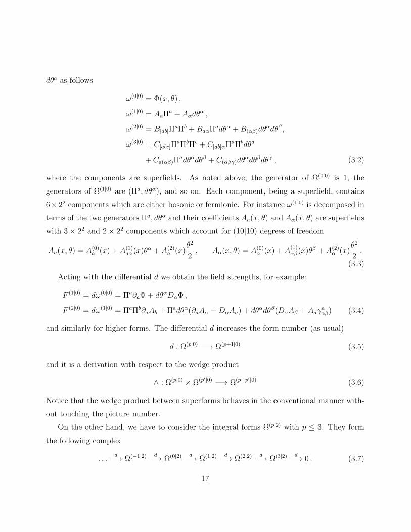
dθa as follows

ω(0|0) = Φ(x, θ) ,

ω(1|0) = AaΠa + Aαdθ

α ,

ω(2|0) = B[ab]ΠaΠb +BaαΠadθα +B(αβ)dθ

αdθβ,

ω(3|0) = C[abc]ΠaΠbΠc + C[ab]αΠaΠbdθa

+ Ca(αβ)Πadθαdθβ + C(αβγ)dθ

αdθβdθγ , (3.2)

where the components are superfields. As noted above, the generator of Ω(0|0) is 1, the

generators of Ω(1|0) are (Πa, dθα), and so on. Each component, being a superfield, contains

6× 22 components which are either bosonic or fermionic. For instance ω(1|0) is decomposed in

terms of the two generators Πa, dθα and their coefficients Aa(x, θ) and Aα(x, θ) are superfields

with 3× 22 and 2× 22 components which account for (10|10) degrees of freedom

Aa(x, θ) = A(0)a (x) + A(1)

aα (x)θα + A(2)a (x)

θ2

2, Aα(x, θ) = A(0)

α (x) + A(1)αβ(x)θβ + A(2)

α (x)θ2

2.

(3.3)

Acting with the differential d we obtain the field strengths, for example:

F (1|0) = dω(0|0) = Πa∂aΦ + dθαDαΦ ,

F (2|0) = dω(1|0) = ΠaΠb∂aAb + Πadθα(∂aAα −DαAa) + dθαdθβ(DαAβ + Aaγaαβ) (3.4)

and similarly for higher forms. The differential d increases the form number (as usual)

d : Ω(p|0) −→ Ω(p+1|0) (3.5)

and it is a derivation with respect to the wedge product

∧ : Ω(p|0) × Ω(p′|0) −→ Ω(p+p′|0) (3.6)

Notice that the wedge product between superforms behaves in the conventional manner with-

out touching the picture number.

On the other hand, we have to consider the integral forms Ω(p|2) with p ≤ 3. They form

the following complex

. . .d−→ Ω(−1|2) d−→ Ω(0|2) d−→ Ω(1|2) d−→ Ω(2|2) d−→ Ω(3|2) d−→ 0 . (3.7)

17

As already discussed in [8], integral forms can admit a negative form degree (by considering

derivatives of the Dirac delta forms), and therefore there is no lower bound in the complex,

but there is an upper bound given by Ω(3|2) which is the 1-dimensional bundle of top forms

(sections of the Berezinian bundle or canonical line bundle).

Again, the forms of this complex can be described locally as follows

ω(3|2) = ΦΠ3δ2(dθ) ,

ω(2|2) = Aa(εabcΠbΠc)δ2(dθ) + AαΠ3ιαδ

2(dθ) ,

ω(1|2) = B[ab](εabcΠc)δ2(dθ) + Baα(εabcΠ

bΠc)ιαδ2(dθ) + B(αβ)Π3ιαιβδ

2(dθ) ,

ω(0|2) = Cδ2(dθ) + C [ab]α(εabcΠc)ιαδ

2(dθ)

+ Ca(αβ)(εabcΠbΠc)ιαιβδ

2(dθ) + C(αβγ)Π3ιαιβιγδ2(dθ) , (3.8)

where the components are superfields and Π3 = εabcΠaΠbΠc. As can be easily seen the

dimensions of these spaces are again (1|0), (3|2), (6|6), . . . , (4p−2|4p−2) where p denotes the

maximum number of derivatives on Dirac delta’s. Again, each term of the decomposition is

a superfield which contains bosonic and fermionic degrees of freedom. The matching of the

dimensions with those of the Ω(3−p|0) forms is due to the duality between the two complexes.

The differential operator d acts on the space of the integral forms as usual increasing the

form number

d : Ω(p|2) −→ Ω(p+1|2) (3.9)

leaving untouched the picture number. Acting on integral forms, one needs the distributional

rules such as dθδ′(dθ) = −δ(dθ) and dθδ(dθ) = 0 to compute their differential.

Among integral forms and between integral forms and superforms, the wedge product is

consistently defined as follows

∧ : Ω(p|2) × Ω(p′|2) −→ 0 , ∧ : Ω(p|2) × Ω(p′|0) −→ Ω(p+p′|2) . (3.10)

The first definition is dictated by the anticommuting properties of delta forms and their

derivatives. If derivatives of delta forms are present, we must take into account also that

δ(dθ)δ′(dθ) = −dθδ′(dθ)δ′(dθ) = 0.

18

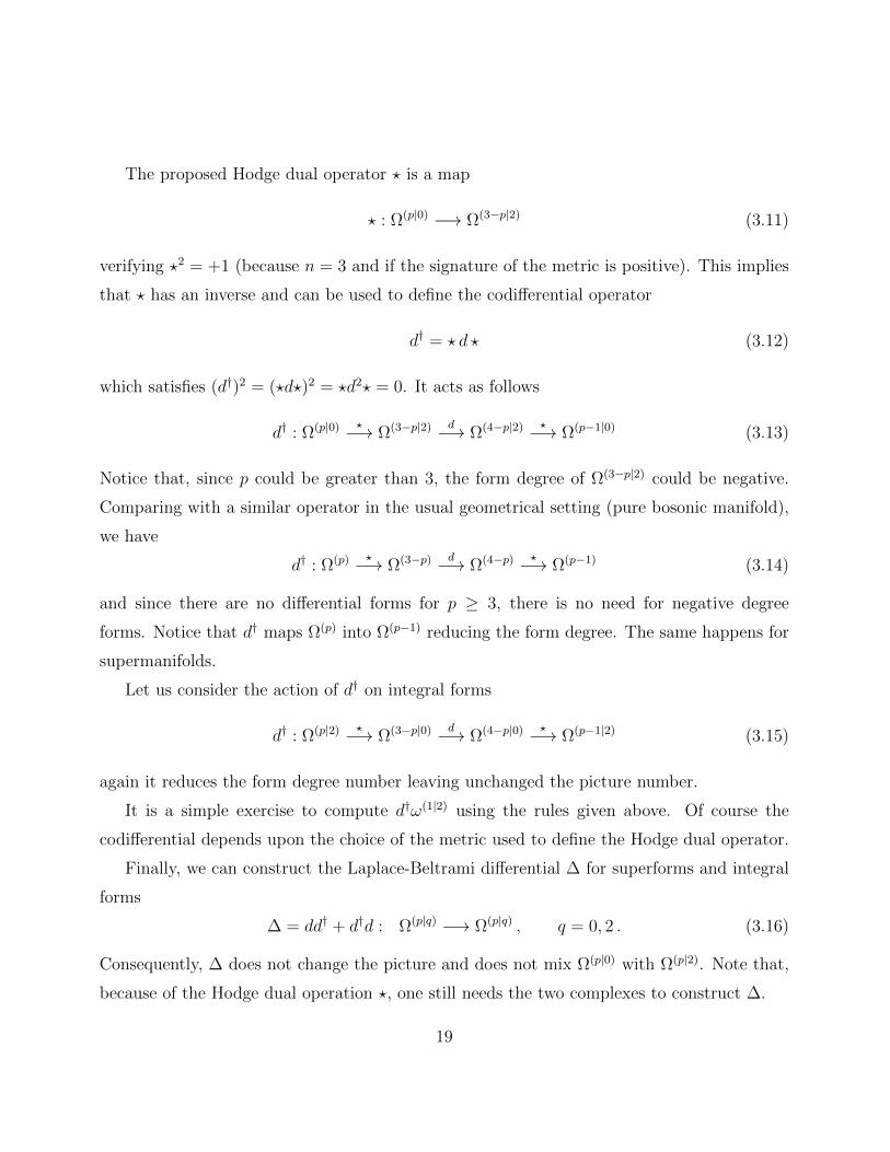
The proposed Hodge dual operator ? is a map

? : Ω(p|0) −→ Ω(3−p|2) (3.11)

verifying ?2 = +1 (because n = 3 and if the signature of the metric is positive). This implies

that ? has an inverse and can be used to define the codifferential operator

d† = ? d ? (3.12)

which satisfies (d†)2 = (?d?)2 = ?d2? = 0. It acts as follows

d† : Ω(p|0) ?−→ Ω(3−p|2) d−→ Ω(4−p|2) ?−→ Ω(p−1|0) (3.13)

Notice that, since p could be greater than 3, the form degree of Ω(3−p|2) could be negative.

Comparing with a similar operator in the usual geometrical setting (pure bosonic manifold),

we have

d† : Ω(p) ?−→ Ω(3−p) d−→ Ω(4−p) ?−→ Ω(p−1) (3.14)

and since there are no differential forms for p ≥ 3, there is no need for negative degree

forms. Notice that d† maps Ω(p) into Ω(p−1) reducing the form degree. The same happens for

supermanifolds.

Let us consider the action of d† on integral forms

d† : Ω(p|2) ?−→ Ω(3−p|0) d−→ Ω(4−p|0) ?−→ Ω(p−1|2) (3.15)

again it reduces the form degree number leaving unchanged the picture number.

It is a simple exercise to compute d†ω(1|2) using the rules given above. Of course the

codifferential depends upon the choice of the metric used to define the Hodge dual operator.

Finally, we can construct the Laplace-Beltrami differential ∆ for superforms and integral

forms

∆ = dd† + d†d : Ω(p|q) −→ Ω(p|q) , q = 0, 2 . (3.16)

Consequently, ∆ does not change the picture and does not mix Ω(p|0) with Ω(p|2). Note that,

because of the Hodge dual operation ?, one still needs the two complexes to construct ∆.

19

Let us construct ∆ for a (0|0)-superform ω(0|0) = Φ(x, θ). We have

∆Φ = (dd† + d†d)Φ = d ? d(

ΦΠ3δ2(dθ))

+ d†(

Πa∂aΦ + dθαDαΦ)

=

= ?d[ √∣∣∣∣detB

detA

∣∣∣∣Aaa′∂aΦεa′b′c′Πb′Πc′δ2(dθ) +

√∣∣∣∣detB

detA

∣∣∣∣Bαα′DαΦΠ3ια′δ2(dθ)

]=

= ?(∂a

(√∣∣∣∣detB

detA

∣∣∣∣Aaa′∂a′Φ)+Dα

(√∣∣∣∣detB

detA

∣∣∣∣Bαα′Dα′Φ

)Π3δ2(dθ)

)=

=

√∣∣∣∣detA

detB

∣∣∣∣(∂a(√∣∣∣∣detB

detA

∣∣∣∣Aaa′∂a′Φ)+Dα

(√∣∣∣∣detB

detA

∣∣∣∣Bαα′Dα′Φ

))(3.17)

which reduces to

∆Φ =(Aaa

′∂a∂a′Φ +Bαα′

DαDα′Φ)

(3.18)

in the case of constant Aaa′

and Bαα′. We remark that the two terms in ∆ are weighted

with two dimensionful matrices in order to take into account the correct dimension of deriva-

tives. As discussed above, this differential operator appears naturally as the differential rep-

resentation of the second order Casimir invariant operator for orthosymplectic and unitary

supergroups.

3.2 Vertical Differentials: Y,Z.

In the present section, we discuss two differential operators relevant in the study of differential

forms in Ω(p|0) and Ω(p|2). They act mapping superforms into integral forms and vice-versa.

The first operator is constructed as follows. Given a constant commuting vector vα we

define the object

Yv = vαθαδ(vβdθ

β) , (3.19)

with the properties

dYv = 0 , Yv 6= dH(−1|1) , δvYv = d(vαθ

αδvβθβδ′(vγdθ

γ)), (3.20)

where H(−1|1) is a pseudoform and δv is a variation of v. Notice that Yv belongs to Ω(0|1) and

by choosing two linear independent vectors v(α), we have

Y =2∏

α=1

Yv(α) = εα1α2θα1θα2εα1α2δ(dθα1)δ(dθα2) = θ2δ2(dθ) . (3.21)

20

which is an integral form of Ω(0|2). The resulting differential operator Y is independent of v’s

since δ(v(1)α dθα)δ(v

(2)β dθβ) = (det(v(1), v(2))−1δ2(dθ) and v

(1)α θα)v

(2)β θβ) = det(v(1), v(2))θ2.

This operator (known as Picture Changing Operator, PCO) changes the picture number

and acts on superforms by the wedge product.

For example, given ω in Ω(p|0) we have

Y : Ω(p|0) −→ Ω(p|2)

ω −→ ω ∧ Y , (3.22)

If dω = 0 then d(ω ∧ Y) = 0 (by applying the Leibniz rule), and if ω 6= dη it follows that

also ω ∧ Y 6= dU where U is an integral form of Ω(p−1|2). In [6], it has been proved that Y is

an element of the de Rham cohomology and is globally defined. So, given an element of the

cohomogy ω ∈ H(p|0)d , the integral form ω ∧ Y is an element of H

(p|2)d .

An important remark: the operator Y being nilpotent Y2 = 0 (because of θαθβθγ = 0 and

because of δ3(dθ) = 0) has a non-trivial kernel; so the operation of raising the picture number

by Y is not an isomorphism between integral and super forms, but only on the cohomologies

therein.

Let us consider again the 2-form F (2|0) = dA(1|0) ∈ Ω(2|0) where A(1|0) = AaΠa + Aαdθ

α ∈Ω(1|0) is a gauge field. Then we can map its field strength F (2|0) into an integral form (which

eventually can be integrated on a (2|2) sub-supermanifold, see [7])

F (2|0) −→ F (2|2) = F (2|0) ∧ Y (3.23)

and satisfies the Bianchi identity dF (2|2) = 0. Using the definition of F (2|0) and using dY = 0,

we have

F (2|2) = d(A(1|0) ∧ Y

)≡ dA(1|2) ,

where A(1|2) = A(1|0) ∧Y is the gauge field at picture number 2. Then, by performing a gauge

transformation on A(1|0), namely δA(1|0) = dλ(0|0), we have

δA(1|2) = d(λ(0|0) ∧ Y

)and therefore λ(0|2) = λ(0|0) ∧ Y is viewed as the gauge parameter at picture number 2.

21

By expanding F (2|0) in components, we have

F (2|0) ∧ Y =(∂aAbΠ

aΠb + · · ·+ (DαAβ + γaαβAa)dθαdθβ

)∧ Y (3.24)

=(∂[aAb](x, 0)θ2

)ΠaΠbδ2(dθ)

where Aa(x, 0) is the lowest component of the superfield Aa appearing in the superconnection

A(1|0). This seems puzzling since we have “killed” the complete superfield (Aa(x, θ), Aα(x, θ))

dependence leaving just the first component Aa(x, 0) = A(0)α (x) as given in (3.3). On the other

side, we have to note that F (2|2) has (3|2) independent superfield components (F a, Fα) while

F (2|0) has (6|6) superfield components (F[ab], Faα, F(αβ)). Analogously, A(1|2) has (6|6) super-

field components (A[ab], Aaα, A(αβ)), while A(1|0) has (3|2) superfield components (Aa, Aα).

To solve this problem we have to modify the definition of picture changing operator given

in (3.19) with a more general construction.

We consider a set of anticommuting superfields Σα(x, θ) such that Σα(x, 0) = 0. They can

be normalised as Σα(x, θ) = θα +Kα(x, θ) with Kα ≈ O(θ2). Then,we define

Y(0|2) =2∏i=1

Σαiδ(dΣαi) =2∏i=1

Σαiδ(

(δαiβ +DβKαi)dθβ + Πa∂aΣ

αi)

(3.25)

=2∏i=1

Σαiδ[(δαiβ +DβK

αi)(dθβ + Πa(1 +DK)−1 β

γ ∂aΣγ)]

=

=1

det(1 +DK)

2∏i=1

Σαiδ[(dθαi + Πa(1 +DK)−1 αi

γ ∂aΣγ)]

where (1 + DK) is a 2 × 2 invertible matrix. Expanding the Dirac delta form and recalling

that the bosonic dimension of the space is 3, we obtain the formula

Y(0|2) = H(x, θ)δ2(dθ) +Kαa (x, θ)Πaιαδ

2(dθ) +

+ La(αβ)(x, θ)εabcΠbΠcιαιβδ

2(dθ) +M (αβγ)(x, θ)Π3ιαιβιγδ2(dθ) , (3.26)

where the superfields H,Kαa , L

a(αβ) and M (αβγ) are easily computed in terms of Σα and its

derivatives. Even if it is not obvious from the final expression in (3.26), Y is closed and not

22

exact from its definition in (3.25). It belongs to Ω(0|2) and it is globally defined; this can be

checked by decomposing the supermanifold in patches and checking that Y is an element of

the Cech cohomology. This was done for example in [6] for super projective varieties. Now, if

we compute the new field strength F (2|2) by (3.23), one sees that the different pieces in (3.26)

from Y pick up different contributions from F (2|0). For instance, the dθα ∧ dθβ is soaked up

from the third piece in (3.26) with the two derivatives acting on Dirac delta function. With

this more general definition of the PCO, all components of F (2|0) appear in the expression of

F (2|0) ∧ Y.

Let us consider now another operator. Taken an odd vector field X = Xa∂a + XαDα

where the coefficients Xa and Xα are fermionic and bosonic, respectively, we define the usual

interior differential (contraction)

ιX = Xαι∂a +XαιDα (3.27)

acting on Ω(p|0) in the conventional way. The anticommuting properties of X imply that

ιXιX 6= 0 (3.28)

which means that ιX is not nilpotent. Therefore, the Cartan calculus has to be modified. A

complete discussion on this point can be found in ref.s [2, 12, 13]. As for the differential dθα,

we need to introduce a distribution-like differential operator to act on δ(dθα) in the same way

as ιa acts on Πb, i.e. ιaΠb = δba (we recall that ιDαdθ

β = δβα, ιadθβ = 0 and ιDαΠb = 0.). We

introduce the operator δ(ιDα) acting as follows

δ(ιDα)δ(dθβ) = δβα . (3.29)

This operator has the property of removing the Dirac delta functions and therefore of changing

the picture by lowering it. To map cohomological classes, we need to modify it in order to be

d closed and not exact. For that we define:

ZX = [d,Θ(ιX)] = δ(ιX)LX +1

2δ′(ιX)ι[X,X] , LX = dιX − ιXd , (3.30)

where Θ(x) is the usual Heaviside (step) function. Again, if we pick up a commuting constant

vector v, we can write the easiest example of ZX by setting X = vα∂α (with X,X = 0) and

23

we have

Zv = δ(ιvα∂α)vα∂α (3.31)

with the properties

dZv = 0 , Zv 6= dH , with H ∈ Ω(−1|2) , δvZv = dη ,with η ∈ Ω(−1|2) (3.32)

Notice that, although Zv can be formally written as d-closed (see eq. (3.30)), Θ(ιX) is not

a Dirac delta form. As in the case of Y, it is convenient to define the product of two Z’s

(defined with two linear independent v’s), to get

Z =2∏i=1

Zv(i) = εαβδ(ια)δ(ιβ)εαβ∂α∂β . (3.33)

where the dependence on v’s drops out. This differential operator acts as follows

Z : Ω(p|2) −→ Ω(p|0)

ω(p|2) −→ Zω(p|2) . (3.34)

As an example, we consider the integral form ω(3|2) = ΦΠ3δ2(dθ) = Φd3xδ2(dθ) (the last

equality is due to the fact that the dependence upon dθ in Π is cancelled because of the

delta’s). Then we find

Z(

Φd3xδ2(dθ))

=(εαβ∂α∂βΦ

)d3x . (3.35)

This example is also useful to show that Z maps cohomologies of H(p|2)d into H

(p|0)d , indeed

since ω(3|2) is automatically closed being a top integral form, we have

d[Z(

Φd3xδ2(dθ))]

= d(εαβ∂α∂βΦ

)d3x = (dxa∂a + dθγ∂γ)

(εαβ∂α∂βΦ

)d3x

= εαβ (∂γ∂α∂βΦ) d3xdθγ = 0 (3.36)

The term of the differential d with the 1-form dxa drops out since the right hand side of (3.35)

is already a three form proportional to d3x and the last equality follows from the fact that

∂α∂β∂γ = 0 since they anticommute. This implies that also Zω(3|2) is closed. In the same way,

for an exact form ω(p|2) = dω(p−1|2), one can show that Zω(0|2) is also exact.

As above, we remark that while Z maps cohomologies into cohomologies, it is not an

isomorphism between integral forms and superforms since it is nilpotent Z2 = 0 (because of

δ3(ιX) = 0 and ∂3 = 0).

24

4 Constraints, Rheonomy and Cohomology

In the present setting, given the complexes of superforms discussed above, we can study the

cohomology of the de Rham operator d and that of d†. The relevant aspect here is that we

can formulate a physical interesting model in two ways, either starting from superforms (as

it has been done so far) or using integral forms. This last procedure might shed new light on

the construction of supersymmetric models.

However, we have to clarify how the cohomology is understood. It is easy to show that

the de Rham cohomology on superforms, by the Poincare lemma coincides with the usual

cohomology

H(d,Ω(n|0)) = Rδn,0 (4.1)

which means that the only closed and not-exact forms are those in the space Ω0|0. However,

in the space of superforms we have the following issue: considering the space of superforms

Ω(1|0), we have two independent sets of superfields Aa(x, θ) and Aα(x, θ), containing several

components. In principle, they could be identified with some physical degrees of freedom,

but, generically, they represent reducible representations of the Lorentz group and therefore

they can be identified with different type of particles. In order to overcome this problem, one

imposes some constraints on the field strength (gauge invariant constraints) in order to reduce

the number of independent components. For example, in the case of A(1|0) (given in 3.2), its

field strength is displayed in (3.4) and denoted by F (2|0). In order to reduce the number of

independent components to the physical ones, the constraint3

ιαιβF(2|0) = (D(αAβ) + γaαβAa) = 0 . (4.2)

must be imposed. Then, by solving with respect to Aa(x, θ), we find that the independent

components are contained in the spinorial part of the connection Aα(x, θ). Condition (4.2) is

an obstruction to the Bianchi identities

dF (2|0) = 0 (4.3)

3In the rheonomic language, this is expressed by the requirement that the component along spinorial “legs”must be expressed in terms of the components along vectorial “legs”. We refer to [14].

25

that can be solved in terms of a single spinorial superfield Wα(x, θ), and we arrive to the final

result (a.k.a. rheonomic parametrisation)

F (2|0) = dA(1|0) = FabΠaΠb + dθγaWΠa ,

dWα = Πa∂aWα − Fab(γabdθ)α + dθαD ,

dD = Πa∂aD + dθγa∂aW . (4.4)

with the relations (obtained by Bianchi’s identities)

∂[aFbc] = 0 ,

∂αFab + (γ[a∂b]W )α = 0 ,

Fab +1

2(γab)

αβDαW

β = 0 ,

DαWα = 0 . (4.5)

The first scalar component of the superfield D is the usual auxiliary field for the off-shell super

gauge fields. Therefore, the constraints (4.2) trasform the Bianchi identities into non-trivial

equations identifying a single field strength Wα and the superfields Aα as the non-trivial

ingredients.

We have to mention the detailed discussion of the cohomology of superforms (based on

the seminal works [15, 11]) provided in [16, 17, 18]. There it is clarified what cohomology

means in the case of superforms and a systematic technique to compute it is provided. This

amounts to fix some of the components of the field strengths to zero and to solve the Bianchi’s

identities. The cohomology is identified as a relative cohomology which is not trivial because

of the additional constraints.

Let us now move to integral forms.4 We have to notice that acting with the differential d,

we move from Ω(p|2) to Ω(p+1|2) increasing the form number and leaving the picture number

4In string theory, the vertex operators needed to construct physical amplitudes are in the BRST cohomologyand they are characterised by two quantum numbers: the ghost number and the picture number. For differentghost number, there are different cohomologies, but at a different picture number (and the same ghost number),there are the same cohomology classes. To be more precise we can choose a representative of the samecohomology class in any picture number. The concept of infinite dimensional complexes of superforms iseasily seen in terms of commuting super ghost fields γ, β.

26

unchanged. However, since the number of independent generators of the spaces Ω(p|2) decreases

as the form number increases, we see that the condition we get by imposing the vanishing

of some field strength components are not enough to reduce to irreducible representations

(usually this consists in finding a single supermultiplet described by a superform). Therefore,

in order to reproduce the relative cohomology of the complex of superforms, we need to use

the new differential d†.

d†A(2|2) = F (1|2) , (4.6)

on which we can finally put the constraints. Notice that the dimension of Ω(2|2) is equal to

the dimension of Ω(1|0), and via the Hodge dual we have a simple mapping of its components

?A(2|2) = Aa ?(εabcΠ

bΠc)δ2(dθ))

+ Aα ?(Π3ιαδ

2(dθ))

=(AaGab + AαGαb

)Πb +

(AaGaβ + AαGαβ

)dθβ . (4.7)

where we have collected all coefficients of the Hodge dual operation as follows

?(εabcΠ

bΠc)δ2(dθ))

= GabΠb + Gaβdθ

β , ?(Π3ιαδ

2(dθ))

= GαbΠb + Gαβdθ

β . (4.8)

At this point we can apply the differential operator d to (4.8) and finally convert it into an

integral form Ω(1|2) by applying again the Hodge dual. The components of d ?F (2|0) are given

by (d ? F (2|0)

)[ab]

= ∂[a(AcG|c|b] + AγGγb]

),(

d ? F (2|0))αb

= ∂a(AcGcα + AγGγα

)−Dα

(AcGca + AγGγa

),(

d ? F (2|0))(αβ)

= D(α

(AcGcβ) + AγG|γ|β)

)+ γaαβ

(AdGda + AγGγa

), (4.9)

Therefore, the constraints needed to select the independent components of the superfield are

given by (d ? F (2|0)

)(αβ)

= 0 . (4.10)

27

4.1 Non-abelian Gauge Fields

Having discussed the constraints to define physical degrees of freedom in terms of a given

superform or integral form, we here discuss how the non-abelian terms are constructed. In

the case of superforms (which we recall are 0-picture forms) the construction is conventional.

Given the superform A(1|0), we consider it with value in a given Lie algebra and we construct

its field strength as follows

F (2|0) = dA(1|0) +1

2[A(1|0), A(1|0)] , (4.11)

where the commutator is taken on the Lie algebra and the two forms are multiplied with the

wedge product. F (2|0) satisfies the Bianchi’s identities

∇AF(2|0) = 0 . (4.12)

where ∇A is the covariant derivative with respect to A(1|0). Notice that multiplying two

0-picture forms, we do not change the global picture. The situation is rather different for

integral forms. Let us consider the 2-picture integral forms A(1|2) with value in a Lie algebra.

We cannot construct the field strength in the usual way since we cannot multiply A(1|2) by

itself (as discussed above). For that we need the PCO Z to reduce the picture first, namely

we consider the 0-picture connection ZA(1|2) and one possible definition is

F (2|2) = dA(1|2) + A(1|2) ∧ ZA(1|2) (4.13)

However, by computing its Bianchi identity, we run into some problems. Indeed, we find

dF (2|2) = dA(1|2) ∧ ZA(1|2) − A(1|2) ∧ dZA(1|2) = dA(1|2) ∧ ZA(1|2) − A(1|2) ∧ ZdA(1|2)

Using the definition (4.13), we get

dF (2|2) =(F (2|2) − A(1|2) ∧ ZA(1|2)) ∧ ZA(1|2) − A(1|2) ∧ Z

(F (2|2) − A(1|2) ∧ ZA(1|2))

= F (2|2) ∧ ZA(1|2) − A(1|2) ∧ ZF (2|2)

− A(1|2) ∧(ZA(1|2) ∧ ZA(1|2) − Z

(A(1|2) ∧ ZA(1|2)

))(4.14)

28

that we can rewrite as

∇ZA(1|2)F (2|2) = ZA(1|2) ∧ F (2|2) − A(1|2) ∧ ZF (2|2)

− A(1|2) ∧(ZA(1|2) ∧ ZA(1|2) − Z

(A(1|2) ∧ ZA(1|2)

))(4.15)

We notice that the first two terms on the right hand side do not cancel since

ZA(1|2) ∧ F (2|2) − A(1|2) ∧ ZF (2|2) 6= 0

which means that Z is not a derivation of the exterior algebra. In addition, notice that

A(1|2) ∧ F (2|2) = 0 by the rule we have established before. For the same reason, we have

ZA(1|2) ∧ ZA(1|2) − Z(A(1|2) ∧ ZA(1|2)

)6= 0 .

A way to solve this problem is to consider the sum of all possible pictures for a 1-form, namely

A = A(1|0) + A(1|1) + A(1|2) where A(1|1) is a pseudo form with a single Dirac delta function.

We have not discussed such an object in the present paper and in the past papers, since they

require some additional studies. In particular, it can be shown that for a given form number

the space of pseudo forms is infinite dimensional. In order to construct A(1|1) we can act on

A(1|2) with a single PCO Zv (introduced in (3.31)) while the relation between A(1|0) and A(1|2)

is obtained by acting with Z which removes both the Dirac delta functions. We construct the

field strength as usual

F = dA+A ∧A =(dA(1|0) + A(1|0) ∧ A(1|0))

+(dA(1|1) + A(1|1) ∧ A(1|0) + A(1|0) ∧ A(1|1))

+(dA(1|2) + A(1|2) ∧ A(1|0) + A(1|1) ∧ A(1|1) + A(1|0) ∧ A(1|2)) , (4.16)

which satisfies by definition to the Bianchi identities

dF (2|0) + F (2|0) ∧ A(1|0) + A(1|0) ∧ F (2|0) = 0 ,

dF (2|1) + F (2|1) ∧ A(1|0) + A(1|0) ∧ F (2|1) + F (2|0) ∧ A(1|1) + A(1|1) ∧ F (2|0) = 0 ,

dF (2|2) + F (2|2) ∧ A(1|0) + F (2|1) ∧ A(1|1) + F (2|0) ∧ A(1|2)

+ A(1|0) ∧ F (2|2) + A(1|1) ∧ F (2|1) + A(1|0) ∧ F (2|2) = 0 . (4.17)

29

The first equation involves only the contribution at zero picture and it is the conventional

expression for the superforms. The other lines invoke the presence of the gauge connection

and of the field strength at different pictures. Notice that for consistency one needs also the

pseudo-forms at picture number equal to one. We conclude that a complete theory of gauge

connections on supermanifolds and non-abelian gauge group is still missing and requires new

methods for dealing with the infinite dimensional spaces of pseudo-forms. This will be studied

in a forthcoming publication.

5 Dualities

Going back to abelian connections, we discuss dualities on supermanifolds. Let us recall what

happens on a bosonic manifold (i.e. R3). We have the complex of differential forms

0d−→ Ω(0) d−→ Ω(1) d−→ Ω(2) d−→ Ω(3) d−→ 0 . (5.1)

Then, if we start with a 0-form A(0), we have the following sequence

A(0) d−→ F (1) = dA(0) ?−→ F (2) = dA(1) (5.2)

We start with a 0-form and we construct its field strength F (1) = dA(0), which obviously

satisfies the Bianchi identity dF (1) = 0. Its field strength is a 1-form. Now, we consider

its Hodge dual, which in three dimensions corresponds to a 2-form F (2). If we require that

the F (2) is closed, the Poincare lemma implies that F (2) = dA(1). However, the closure of

F (2) implies the co-closure of F (1), namely d ? F (1) = 0. This, combined with the Bianchi

identities, implies d ? dA(0) = 0 which is the Klein-Gordon equation in three dimensions. On

the other side, we have that the Bianchi identities for F (1) imply also that d?F (2) = 0, which,

combined with its Bianchi identities, leads to d ? dA(1) = 0 which is the Maxwell equation

for a vector field. Together with the gauge invariance of A(1), namely δA(1) = dλ(0), we

have that A(1) describes a single propagating degree of freedom for a massless gauge boson in

three dimensions. This is the basic argument for the duality between a scalar field in three

dimensions and a massless gauge boson.

30

In the same way, one can easily prove that in three dimensions there are no higher p-forms

with propagating degrees of freedom. Indeed, if one starts from a 2-form A(2), its field strength

is a 3-form F (3) and its Hodge dual is a 0-form, implying that there is no propagating degree

of freedom. Notice that this argument works for on-shell fields. This is essential to guarantee

the correct matching of degrees of freedom in each multiplet.

In the case of supermanifolds, there is the problem of the unboundness of the complex of

superforms. Therefore, it is not clear whether additional propagating supermultiplets can be

described by higher rank p-superforms. On the other side, we know that the physical content

of the complex of superforms should be mirrored into the complex of integral forms.

If we start from a (0|0)-form A(0|0), which describes a scalar superfield with (2|2) degrees of

freedom (as can be checked easily by counting the independent coefficients of the θ expansion),

we can build its field strength as above

A(0|0) d−→ F (1|0) = dA(0|0) ?−→ F (2|2) = dA(1|2) (5.3)

The resulting superform F (1|0) = dA(0|0) satisfies the Bianchi identities. Consequently, the

Hodge dual F (2|2) is an integral form and its closure implies its exactness by the Poincare

lemma which is valid in the case of Ω(p|2) with p > 0 . Then, by repeating the same argument

as above, we have that the Bianchi identity on F (2|2) implies the equation

d ? dA(0|0) = 0 , (5.4)

namely, it leads to a modified Klein-Gordon equation (with high derivative terms (see [9]). It

describes a scalar superfield with high derivative terms. On the other hand, we have that the

Bianchi identity on F (1|0) implies the following equation

d ? dA(1|2) = 0 . (5.5)

One finds that it describes an on-shell gauge supermultiplet (made by one bosonic degree of

freedom and one fermionic degree of freedom). The on-shell condition, the supersymmetry and

the gauge symmetry guarantee that indeed we are describing such a supermultiplet. We have

to notice that this is not the usual representation of a gauge supermultiplet (which is normally

31

described by a (1|0) superform A(1|0)) and that it corresponds to the mirror representation in

terms of integral forms of the same multiplets contained in the complex of superforms.

On the other hand, if we start from the conventional superform A(1|0) for a gauge multiplet,

we have the following sequence

A(1|0) d−→ F (2|0) = dA(1|0) ?−→ F (1|2) = dA(0|2) (5.6)

where A(0|2) is a (0|2) integral form. Again, by exploiting the Bianchi identities on both sides

of the Hodge duality, we find the equivalence between the two descriptions.

Finally, let us study what happens if we further increase the form number (which is indeed

possible without any restriction in the case of superforms). We have

A(p|0) d−→ F (p+1|0) = dA(p|0) ?−→ F (2−p|2) = dA(1−p|2) (5.7)

If p ≥ 2, we see that A(1−p|2) belongs to the space of integral forms with negative form degree.

However, this space cannot contain any physical degree of freedom since, by means of the

PCO operators (which map physical degrees of freedom into physical degrees of freedom) we

see that there is no room for any physical content in that space. Thus, we conclude that

higher-rank A(p|0) superforms cannot describe on-shell degrees of freedom consistently in the

bosonic three dimensional case.

This construction resolves the issues of higher rank superforms and the description of dual

superfields.

Summary

We have generalized the construction of the Hodge dual via Fourier transform given in a

previous work. We apply the Hodge dual theory to construct the Laplace-Beltrami differential

and to analise the Hodge dualities in supersymmetric models. We discuss the relation between

superspace constraints for superforms and for integral forms. In addition, we discuss the

relation between integral forms and superforms via PCO’s and, in that framework, we consider

non-abelian gauge fields in the space of integral forms.

32

References

[1] T. Voronov and A. Zorich: “Integral transformations of pseudodifferential forms”, Usp.

Mat. Nauk, 41 (1986) 167-168; T. Voronov and A. Zorich: “Complex of forms on a super-

manifold”, Funktsional. Anal. i Prilozhen., 20 (1986) 58-65; T. Voronov and A. Zorich:

“Theory of bordisms and homotopy properties of supermanifolds”, Funktsional. Anal. i

Prilozhen., 21 (1987) 77-78; T. Voronov and A. Zorich: “Cohomology of supermanifolds

and integral geometry”, Soviet Math. Dokl., 37 (1988) 96-101.

[2] A. Belopolsky, “New geometrical approach to superstrings”, [arXiv:hep-th/9703183].

A. Belopolsky, “Picture changing operators in supergeometry and superstring theory”,

[arXiv:hep-th/9706033].

[3] N. Berkovits, “Multiloop amplitudes and vanishing theorems using the pure spinor for-

malism for the superstring,” JHEP 0409 (2004) 047 [hep-th/0406055].

[4] N. Berkovits and W. Siegel, “Regularizing Cubic Open Neveu-Schwarz String Field The-

ory,” JHEP 0911 (2009) 021 [arXiv:0901.3386 [hep-th]].

[5] R. Catenacci, M. Debernardi, P. A. Grassi and D. Matessi, “Balanced Superprojective

Varieties”, J. Geo. and Phys. Volume 59, Issue 10 (2009) p. 1363-1378. [arXiv:0707.4246

[hep-th]].

[6] R. Catenacci, M. Debernardi, P. A. Grassi and D. Matessi, “Cech and de Rham Coho-

mology of Integral Forms,” J. Geom. Phys. 62 (2012) 890 [arXiv:1003.2506 [math-ph]].

[7] E. Witten, “Notes On Supermanifolds and Integration,” arXiv:1209.2199 [hep-th].

[8] L. Castellani, R. Catenacci and P. A. Grassi, “Supergravity Actions with Integral Forms,”

Nucl. Phys. B 889, 419 (2014) [arXiv:1409.0192 [hep-th]].

[9] L. Castellani, R. Catenacci and P. A. Grassi, “The Geometry of Supermanifolds and New

Supersymmetric Actions,” arXiv:1503.07886 [hep-th].

33

[10] L. Dolan and E. Witten, “Vertex operators for AdS(3) background with Ramond-Ramond

flux,” JHEP 9911, 003 (1999) [hep-th/9910205].

[11] S. J. Gates, M. T. Grisaru, M. Rocek and W. Siegel, “Superspace Or One Thousand and

One Lessons in Supersymmetry,” Front. Phys. 58, 1 (1983) [hep-th/0108200].

[12] P. A. Grassi and G. Policastro, “Super-Chern-Simons theory as superstring theory,” hep-

th/0412272.

[13] P. A. Grassi and M. Marescotti, “Integration of Superforms and Super-Thom Class,”

arXiv:0712.2600 [hep-th].

[14] L. Castellani, R. D’Auria and P. Fre, “Supergravity and superstrings: A Geometric

perspective,” in 3 vol.s, Singapore: World Scientific (1991) 1375-2162;

[15] S. J. Gates, Jr., “Super P Form Gauge Superfields,” Nucl. Phys. B 184, 381 (1981).

[16] W. D. Linch and S. Randall, “Superspace de Rham Complex and Relative Cohomology,”

arXiv:1412.4686 [hep-th].

[17] S. Randall, “The Structure of Superforms,” arXiv:1412.4448 [hep-th].

[18] S. J. Gates, W. D. Linch and S. Randall, “Superforms in Five-Dimensional, N = 1

Superspace,” arXiv:1412.4086 [hep-th].

34