1

HOCKEY STICKS, PRINCIPAL COMPONENTS AND SPURIOUS SIGNIFICANCE

Stephen McIntyre 512-120 Adelaide St. West,

Toronto, Ontario Canada M5H 1T1 stephen.mcintyre@utoronto.ca

Ross McKitrick Department of Economics,

University of Guelph, Guelph Ontario Canada N1G 2W1.

2

HOCKEY STICKS, PRINCIPAL COMPONENTS AND SPURIOUS SIGNIFICANCE

ABSTRACT

The “hockey stick” shaped temperature reconstruction of Mann et al. [1998, 1999] has been widely applied. However it has not been previously noted in print that, prior to their principal components (PCs) analysis on tree ring networks, they carried out an unusual data transformation which strongly affects the resulting PCs. Their method, when tested on persistent red noise, nearly always produces a hockey stick shaped first principal component (PC1) and overstates the first eigenvalue. In the controversial 15th century period, the MBH98 method effectively selects only one species (bristlecone pine) into the critical North American PC1, making it implausible to describe it as the “dominant pattern of variance”. Through Monte Carlo analysis, we show that MBH98 benchmarks for significance of the Reduction of Error (RE) statistic are substantially under-stated and, using a range of cross-validation statistics, we show that the MBH98 15th century reconstruction lacks statistical significance.

3

HOCKEY STICKS, PRINCIPAL COMPONENTS AND SPURIOUS SIGNIFICANCE

1. INTRODUCTION

The term “hockey stick” is often used to describe the shape of the Northern Hemisphere (NH)

mean temperature index introduced in Mann et al. [1998, hereinafter “MBH98”]. For

convenience, we define the “hockey stick index” of a series as the difference between the mean

of the closing sub-segment (here 1902-1980) and the mean of the entire series (typically 1400-

1980 in this discussion) in units of the long-term standard deviation (σ), and a “hockey stick

shaped” series is defined as one having a hockey stick index of at least 1 σ. Such series may be

either upside-up (i.e. the “blade” trends upwards) or upside-down. Our focus here is on the 1400-

1450 step (“AD1400 step”) of MBH98, because of controversy over early 15th century

temperature reconstructions [McIntyre and McKitrick, 2003; Mann et al., 2003]. Our particular

interest in the performance of the Reduction of Error (RE) statistic arises out of that controversy.

We also focus on the North American tree ring network (“NOAMER”), because the first

principal component (“PC1”) of this network has been identified as essential for controversial

periods of the MBH98 temperature reconstruction [Mann et al., 1999, 2003]. MBH98 has

recently been criticized on other grounds in von Storch et al. [2004].

MBH98 used principal components (PCs) to reduce the dimensionality of tree ring networks and

stated that they used “conventional” PC analysis. A conventional PC algorithm centers the data

by subtracting the column means of the underlying series. For the AD1400 step highlighted here,

this would be the full 1400-1980 interval. Instead, MBH98 Fortran code

(ftp://holocene.evsc.edu/pub/MBH98/TREE/ITRDB/NOAMER/pca-noamer) contains an

unusual data transformation prior to PC calculation that has never been reported in print. Each

4

tree ring series was transformed by subtracting the 1902-1980 mean, then dividing by the 1902-

1980 standard deviation and dividing again by the standard deviation of the residuals from fitting

a linear trend in the 1902-1980 period. The PCs were then computed using singular value

decomposition on the transformed data. (The effects reported here would have been partly

mitigated if PCs had been calculated using the covariance or correlation matrix.) This previously

unreported transformation was recently acknowledged in the Supplementary Information to a

Corrigendum to MBH98 [Mann et al. 2004a], where they asserted that it has no effect on the

results, a claim we refute herein.

PCs can be strongly affected by linear transformations of the raw data. Under the MBH98

method, for those series in which the 1902-1980 mean is close to the 1400-1980 mean,

subtraction of the 1902-1980 mean has little impact on weightings for the PC1. But if the 1902-

1980 mean is different than the 1400-1980 mean (i.e. a hockey stick shape), the transformation

translates the “shaft” off a zero mean; the magnitude of the residuals along the shaft is increased,

and the series variance, which grows with the square of each residual, gets inflated. Since PC

algorithms choose weights that maximize variance, the method re-allocates variance so that

hockey stick shaped series get overweighted. In effect, the MBH98 data transformation results in

the PC algorithm mining the data for hockey stick patterns.

In a network of persistent red noise, there will be some series that randomly “trend” up or down

during the ending sub-segment of the series (as well as other sub-segments). In the next section,

we discuss a Monte Carlo experiment to show that these spurious “trends” in a closing segment

are sufficient for the MBH98 method, when applied to a network of red noise, to yield hockey

5

stick PC1s, even though the underlying data generating process has no trend component. We

then examine the effect of this procedure on actual MBH98 weights for the North American

PC1. Finally we use the simulated PC1s to establish benchmarks for the Reduction of Error (RE)

verification statistic used in MBH98, and we discuss R2 and other verification statistics for the

MBH98 reconstruction.

2. MONTE CARLO SIMULATIONS OF HOCKEY STICKS ON TRENDLESS

PERSISTENT SERIES

We generated the red noise network for Monte Carlo simulations as follows. We downloaded

and collated the NOAMER tree ring site chronologies used in MBH98 from M. Mann’s FTP site

and selected the 70 sites used in the AD1400 step. We calculated autocorrelation functions for all

70 series for the 1400-1980 period. For each simulation, we applied the algorithm hosking.sim

[Whitcher, 2003], which applied a method due to Hosking [1984] to simulate trendless red noise

based on the complete auto-correlation function. All simulations and other calculations were

done in R [R Development Core Team, 2004]. Computer scripts used to generate simulations,

figures and statistics are available at <ftp://ftp.agu.org/apend/gl/2004GL021750>, together with

a sample of 100 simulated “hockey sticks” and other supplementary information. We carried out

10,000 simulations, in each case obtaining 70 stationary series of length 581 (corresponding to

the 1400-1980 period). By the very nature of the simulation, there were no 20th century trends,

other than spurious “trends” from persistence. We applied the MBH98 data transformation to

each series in the network: the 1902-1980 mean was subtracted, then the series was divided by

the 1902-1980 standard deviation, then by the 1902-1980 detrended standard deviation. We

6

carried out a singular value decomposition on the 70 transformed series (following MBH98) and

saved the PC1 from each calculation.

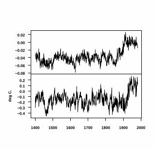
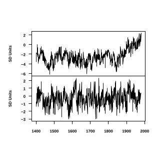
The simulations nearly always yielded PC1s with a hockey stick shape, some of which bore a

quite remarkable similarity to the actual MBH98 temperature reconstruction – as shown by the

example in Figure 1 below. A sharp inflection was regularly observed at the start of the 1902-

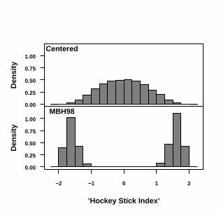
1980 “calibration period”. Figure 2 shows histograms of the hockey stick index of the simulated

PC1s. Without the MBH98 transformation (top panel), a 1 σ hockey stick occurs in the PC1 only

15.3% of the time (1.5 σ - 0.1% ). Using the MBH98 transformation (bottom panel), a 1 σ

hockey stick occurs over 99% of the time, (1.5 σ – 73%; 1.75 σ – 21% and 2σ – 0.2%).

[Figure 1 here]

[Figure 2 here]

The hockey sticks were upside-up about half the time and upside-down half the time, but the

1902-1980 mean is almost never within one σ of the 1400-1980 mean under the MBH98 method.

PC series have no inherent orientation and, since the MBH98 methodology uses proxies

(including the NOAMER PC1) in a regression calculation, the fit of the regression is indifferent

to whether the hockey stick is upside-up or upside-down. In the latter case, the slope coefficient

is negative. In fact, the North American PC1 in Mann et al. [1999] is an upside-down hockey

stick, as shown at

<ftp://ftp.ngdc.noaa.gov/paleo/contributions_by_author/mann1999/proxies/itrdb-namer-

pc1.dat>.

7

The loadings on the first eigenvalues were inflated by the MBH98 method. Without the

transformation, the median fraction of explained variance of the PC1 was only 4.1% (99th

percentile - 5.5%). Under the MBH98 transformation, the median fraction of explained variance

from PC1 was 13% (99th percentile - 23%), often making the PC1 appear to be a “dominant”

signal, even though the network is only noise.

3. THE PC1 IN THE MBH98 NORTH AMERICAN NETWORK

We now show the effect of the MBH98 algorithm on the actual NOAMER network in the

controversial AD1400 step.

Without the data transformation the PC1 is very similar to the unweighted mean of all the series

and, as shown in the top panel of Figure 3, does not have a hockey stick shape. However, under

the MBH98 algorithm, the PC1 has a marked hockey stick shape, as shown in the bottom panel

of Figure 3. The MBH98 method creates a PC1 which is dominated by bristlecone pines and

closely related foxtail pines. (Foxtail pines are located in an adjacent mountain range, interbreed

with bristlecone pines and are included here with bristlecone pines collectively). Out of 70 sites

in the network, 93% of the variance in the MBH98 PC1 is accounted for by only 15 bristlecone

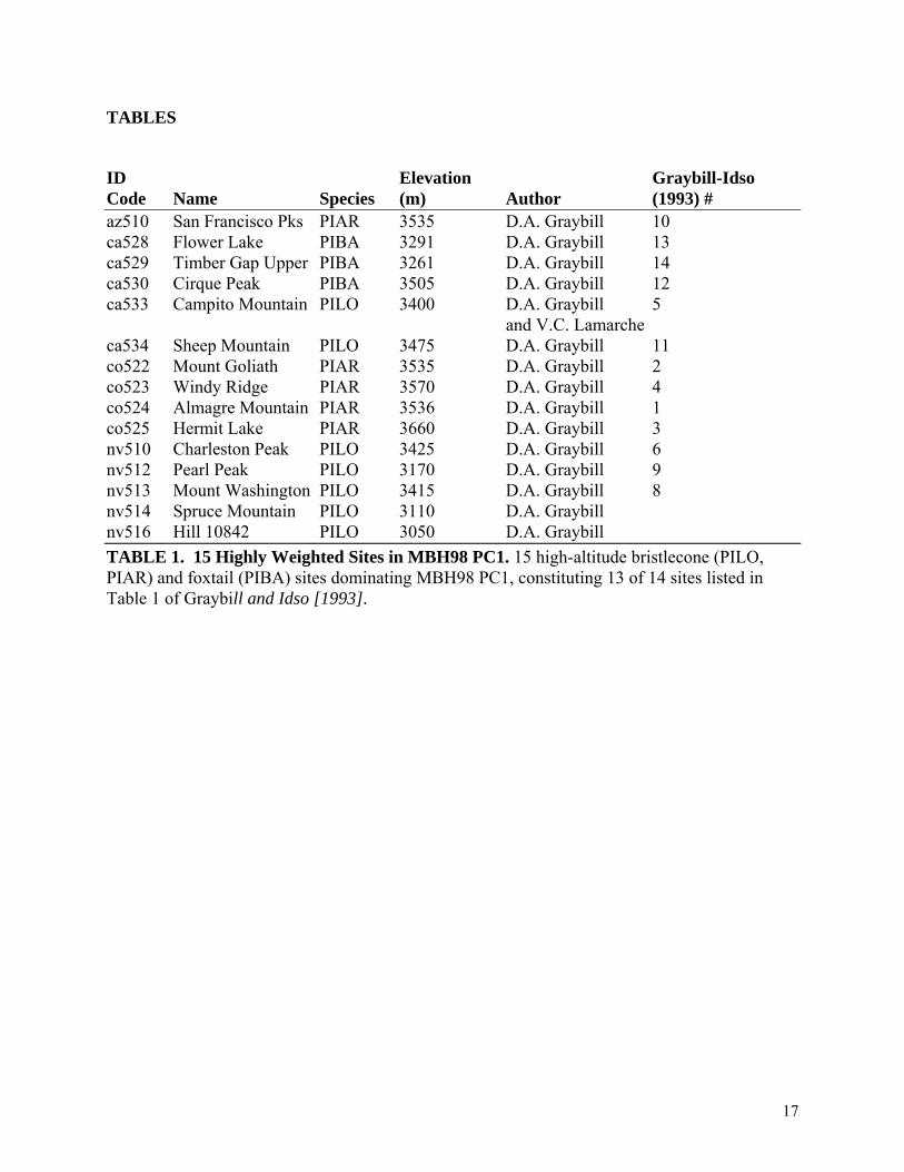
and foxtail pine sites collected by Donald Graybill [Graybill and Idso, 1993; see Table 1]. The

weights in the MBH98 PC1 have a nearly linear relationship to the hockey stick index. The most

heavily weighted site in the MBH98 PC1, Sheep Mountain, is a bristlecone pine site with the

most pronounced hockey stick shape (1.6 σ) in the network; it receives over 390 times the weight

of the least weighted site, Mayberry Slough, whose hockey stick index is near 0.

8

[ Table 1 here]

[Figure 3 here]

Under the MBH98 data transformation, the distinctive contribution of the bristlecone pines is in

the PC1, which has a spuriously high explained variance coefficient of 38% (without the

transformation – 18%). Without the data transformation, the distinctive contribution of the

bristlecones only appears in the PC4, which accounts for less than 8% of the total explained

variance.

This substantially reduced share of explained variance, together with the fact that species other

than bristlecone/foxtail pines are effectively omitted from the MBH98 PC1, argues strongly

against interpreting it as the “dominant component of variance” in the North American network

[Mann et al, 2004b]. In McIntyre and McKitrick [2005, forthcoming], we discuss, inter alia,

problems relating to the interpretation of bristlecone/foxtail pine growth as a temperature proxy,

and we show the impact of using conventional (centered) PC methods on the MBH98 northern

hemisphere temperature index, which has a significant effect on the relative values in the 15th

and 20th centuries.

3. BENCHMARKING THE REDUCTION OF ERROR STATISTIC FOR THE MBH98

ALGORITHM

In most dendroclimatic studies several verification statistics are used. For example, Cook et al.

[1994] describes the Reduction of Error (RE), R2, Coefficient of Efficiency (CE), sign test and

9

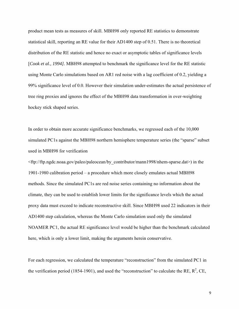
product mean tests as measures of skill. MBH98 only reported RE statistics to demonstrate

statistical skill, reporting an RE value for their AD1400 step of 0.51. There is no theoretical

distribution of the RE statistic and hence no exact or asymptotic tables of significance levels

[Cook et al., 1994]. MBH98 attempted to benchmark the significance level for the RE statistic

using Monte Carlo simulations based on AR1 red noise with a lag coefficient of 0.2, yielding a

99% significance level of 0.0. However their simulation under-estimates the actual persistence of

tree ring proxies and ignores the effect of the MBH98 data transformation in over-weighting

hockey stick shaped series.

In order to obtain more accurate significance benchmarks, we regressed each of the 10,000

simulated PC1s against the MBH98 northern hemisphere temperature series (the “sparse” subset

used in MBH98 for verification

<ftp://ftp.ngdc.noaa.gov/paleo/paleocean/by_contributor/mann1998/nhem-sparse.dat>) in the

1901-1980 calibration period – a procedure which more closely emulates actual MBH98

methods. Since the simulated PC1s are red noise series containing no information about the

climate, they can be used to establish lower limits for the significance levels which the actual

proxy data must exceed to indicate reconstructive skill. Since MBH98 used 22 indicators in their

AD1400 step calculation, whereas the Monte Carlo simulation used only the simulated

NOAMER PC1, the actual RE significance level would be higher than the benchmark calculated

here, which is only a lower limit, making the arguments herein conservative.

For each regression, we calculated the temperature “reconstruction” from the simulated PC1 in

the verification period (1854-1901), and used the “reconstruction” to calculate the RE, R2, CE,

10

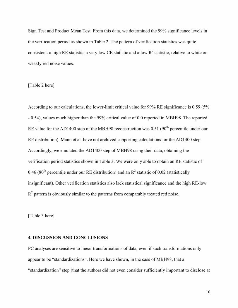
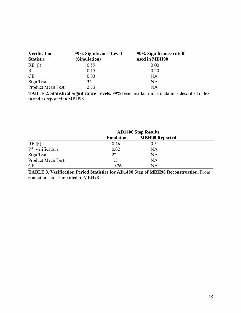
Sign Test and Product Mean Test. From this data, we determined the 99% significance levels in

the verification period as shown in Table 2. The pattern of verification statistics was quite

consistent: a high RE statistic, a very low CE statistic and a low R2 statistic, relative to white or

weakly red noise values.

[Table 2 here]

According to our calculations, the lower-limit critical value for 99% RE significance is 0.59 (5%

- 0.54), values much higher than the 99% critical value of 0.0 reported in MBH98. The reported

RE value for the AD1400 step of the MBH98 reconstruction was 0.51 (90th percentile under our

RE distribution). Mann et al. have not archived supporting calculations for the AD1400 step.

Accordingly, we emulated the AD1400 step of MBH98 using their data, obtaining the

verification period statistics shown in Table 3. We were only able to obtain an RE statistic of

0.46 (80th percentile under our RE distribution) and an R2 statistic of 0.02 (statistically

insignificant). Other verification statistics also lack statistical significance and the high RE-low

R2 pattern is obviously similar to the patterns from comparably treated red noise.

[Table 3 here]

4. DISCUSSION AND CONCLUSIONS

PC analyses are sensitive to linear transformations of data, even if such transformations only

appear to be “standardizations”. Here we have shown, in the case of MBH98, that a

“standardization” step (that the authors did not even consider sufficiently important to disclose at

11

the time of their study) significantly affected the resulting PC series. Indeed, the effect of the

transformation is so strong that a hockey-stick shaped PC1 is nearly always generated from

(trendless) red noise with the persistence properties of the North American tree ring network.

This result is disquieting, given that the NOAMER PC1 has been reported to be essential to the

shape of the MBH98 Northern Hemisphere temperature reconstruction.

For evaluation of statistical skill in paleoclimatic studies, the Reduction of Error (RE) statistic is

widely used, but lacks a theoretical distribution. Practitioners use Monte Carlo models to

establish significance benchmarks. Here we have shown that the benchmarks can be dramatically

affected by the Monte Carlo model itself and that the 99% significance level from a Monte Carlo

model more accurately representing actual MBH98 procedures is 0.59, as compared to the level

of 0.0 reported in the original study. More generally, this example shows that changes in

methodology will generally require new Monte Carlo modeling, that benchmarks carried forward

from one methodology cannot necessarily be applied to a new methodology – even if the method

changes may appear slight, and that great caution is required prior to concluding statistical

significance based on RE statistics.

An obvious guard against spurious RE significance is to examine other cross-validation

statistics, such as the R2 and CE statistics, as recommended, for example, in Cook et al. [1994].

While there are limitations to the R2 statistic, the analysis of statistical “skill” of Murphy [1988]

presupposes that the R2 statistic exceeds the skill statistic and cases where the RE statistic

exceeds the R2 statistic are of particular concern [Cook et al., 1994]. In the case of MBH98,

unfortunately, neither the R2 and other cross-validation statistics nor the underlying construction

12

step have ever been reported for the controversial 15th century period. Our calculations have

indicated that they are statistically insignificant. Timely reporting of these statistics (in the

original article) might have led to an earlier consideration of the discrepancy between the

apparently high RE value and the low values of other statistics, and thus enabled earlier

identification of the underlying data transformation resulting in this problem.

13

Acknowledgments

No funding was sought or received for this work.

14

REFERENCES

Cook, E.R., Briffa, K.R. and Jones, P.D. (1994), Spatial regression methods in dendroclimatology: a review and comparison of two techniques. Int. J. of Climatol., 14, 379-402.

Graybill, D.A., and S.B. Idso (1993), Detecting the aerial fertilization effect of atmospheric CO2 enrichment in tree-ring chronologies, Global Biogeochemical Cycles, 7, 81-95.

Hosking, J. R. M. (1984), Modeling persistence in hydrological time series using fractional differencing, Water Resources Research, 20(12), 1898-1908.

Hughes, M.K. and G. Funkhouser (2003), Frequency-dependent climate signal in upper and lower forest border trees in the mountains of the Great Basin. Climatic Chang, 59, 233-244

Mann, M.E., R.S. Bradley and M.K. Hughes (1998), Global-scale temperature patterns and climate forcing over the past six centuries, Nature, 392, 779-787.

Mann, M.E., R.S. Bradley and M.K. Hughes (1999), Northern Hemisphere temperatures during the past millennium: Inferences, Uncertainties, and Limitations, Geophys. Res. Let., 26, 759-762.

Mann, M.E., R.S. Bradley and M.K. Hughes (2003), Note on Paper by McIntyre and McKitrick in Energy and Environment, ftp://holocene.evsc.virginia.edu/pub/mann/EandEPaperProblem.pdf

Mann, M.E., R.S. Bradley and M.K. Hughes (2004a), Corrigendum: Global-scale temperature patterns and climate forcing over the past six centuries, Nature, 430, 105.

Mann, M.E., R.S. Bradley and M.K. Hughes (2004b), REPLY TO "Global-scale temperature patterns and climate forcings over the past six centuries: A comment" by S. McIntyre and R. McKitrick, Retrieved from website of Stephen Schneider <http://stephenschneider.stanford.edu/Publications/PDF_Papers/MannEtAl2004.pdf>.

McIntyre, S. and R. McKitrick (2003), Corrections to the Mann et. al. (1998) Proxy Data Base and Northern Hemispheric Average Temperature Series, Energy and Environment 14, 751-771.

McIntyre, S. and R. McKitrick (2005), The M&M Critique of the MBH98 Northern Hemisphere Climate Index: Update and Implications, Energy and Environment forthcoming.

Murphy, Allan H. (1988), Skill Scores Based on the Mean Square Error and Their Relationships to the Correlation Coefficient, Monthly Weather Review 116, 2417-2424.

R Development Core Team (2004), R: A language and environment for statistical computing. R Foundation for Statistical Computing, Vienna, Austria. ISBN 3-900051-00-3, <http://www.R-project.org>.

von Storch, H., E. Zorita, J.M. Jones, Y. Dimitriev, F. González-Rouco and S.F.B. Tett (2004), Reconstructing Past Climate from Noisy Data, Science 306, 679-682.

15

Whitcher, Brandon (2003), The waveslim Package: Basic wavelet routines for one-, two- and three-dimensional signal processing, <cran.r-project.org/doc/packages/waveslim.pdf>

16

FIGURE CAPTIONS

FIGURE 1. Simulated and MBH98 Hockey Stick Shaped Series. Top: Sample PC1 from

Monte Carlo simulation using the procedure described in text applying MBH98 data

transformation to persistent trendless red noise; Bottom: MBH98 Northern Hemisphere

temperature index re-construction.

FIGURE 2. Histogram of 'Hockey Stick Index' for PC1s. For the 10,000 simulated PC1s

described in text, the histogram shows the distribution of the difference between the 1902-1980

mean and the 1400-1980 mean, divided by the 1400-1980 standard deviation. Top: Conventional

(centered) calculation; Bottom: with MBH98 data transformation.

FIGURE 3. PC1 for AD1400 North American Tree Ring Network. Top: Result with MBH98

data transformation; Bottom: recalculated on the same data without MBH98 data transformation.

Both standardized to 1902-1980 period.

17

TABLES

ID Elevation Graybill-Idso Code Name Species (m) Author (1993) # az510 San Francisco Pks PIAR 3535 D.A. Graybill 10 ca528 Flower Lake PIBA 3291 D.A. Graybill 13 ca529 Timber Gap Upper PIBA 3261 D.A. Graybill 14 ca530 Cirque Peak PIBA 3505 D.A. Graybill 12 ca533 Campito Mountain PILO 3400 D.A. Graybill 5 and V.C. Lamarche ca534 Sheep Mountain PILO 3475 D.A. Graybill 11 co522 Mount Goliath PIAR 3535 D.A. Graybill 2 co523 Windy Ridge PIAR 3570 D.A. Graybill 4 co524 Almagre Mountain PIAR 3536 D.A. Graybill 1 co525 Hermit Lake PIAR 3660 D.A. Graybill 3 nv510 Charleston Peak PILO 3425 D.A. Graybill 6 nv512 Pearl Peak PILO 3170 D.A. Graybill 9 nv513 Mount Washington PILO 3415 D.A. Graybill 8 nv514 Spruce Mountain PILO 3110 D.A. Graybill nv516 Hill 10842 PILO 3050 D.A. Graybill TABLE 1. 15 Highly Weighted Sites in MBH98 PC1. 15 high-altitude bristlecone (PILO, PIAR) and foxtail (PIBA) sites dominating MBH98 PC1, constituting 13 of 14 sites listed in Table 1 of Graybill and Idso [1993].

18

Verification 99% Significance Level 99% Significance cutoff Statistic (Simulation) used in MBH98 RE (β) 0.59 0.00 R2 0.15 0.20 CE 0.03 NA Sign Test 32 NA Product Mean Test 2.73 NA TABLE 2. Statistical Significance Levels. 99% benchmarks from simulations described in text in and as reported in MBH98.

AD1400 Step Results Emulation MBH98 Reported RE (β) 0.46 0.51 R2- verification 0.02 NA Sign Test 22 NA Product Mean Test 1.54 NA CE -0.26 NA TABLE 3. Verification Period Statistics for AD1400 Step of MBH98 Reconstruction. From emulation and as reported in MBH98.

−0.08

−0.06

−0.04

−0.02

0.00

0.02

deg

C.

−0.4−0.3−0.2−0.1

0.00.10.2

1400 1500 1600 1700 1800 1900 2000

Den

sity

0.00

0.25

0.50

0.75

1.00Centered

’Hockey Stick Index’

Den

sity

−2 −1 0 1 2

0.00

0.25

0.50

0.75

1.00MBH98

SD

Un

its

−6

−4

−2

0

2

SD

Un

its

−3

−2

−1

0

1

2

1400 1500 1600 1700 1800 1900 2000