![Punjabi Pos Tagger: Rule Based and HMM...Sapna Kanwar[7] developed HMM based part of speech tagger for Punjabi. Bi-Gram HMM model was used to build this system. Accuracy of the system](https://static.fdocuments.in/doc/165x107/611945c139acac58f33364c1/punjabi-pos-tagger-rule-based-and-sapna-kanwar7-developed-hmm-based-part.jpg)
HMM - Part 2
34
1 HMM - Part 2 The EM algorithm Continuous density HMM
-
Upload
aimee-william -
Category
Documents
-
view
54 -
download
0
description
HMM - Part 2. The EM algorithm Continuous density HMM. The EM Algorithm. EM: Expectation Maximization Why EM? Simple optimization algorithms for likelihood functions rely on the intermediate variables, called latent data For HMM , the state sequence is the latent data - PowerPoint PPT Presentation
Transcript of HMM - Part 2
1
HMM - Part 2
The EM algorithm Continuous density HMM
2
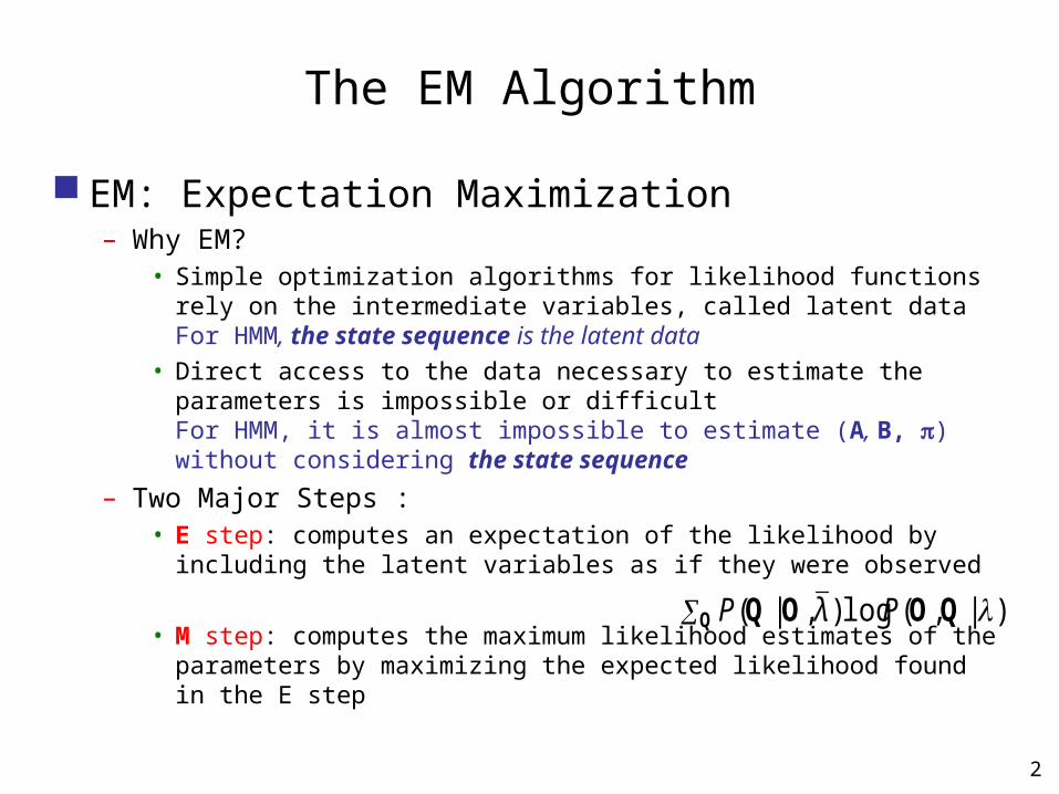
The EM Algorithm
EM: Expectation Maximization– Why EM?
• Simple optimization algorithms for likelihood functions rely on the intermediate variables, called latent dataFor HMM, the state sequence is the latent data
• Direct access to the data necessary to estimate the parameters is impossible or difficultFor HMM, it is almost impossible to estimate (A, B, ) without considering the state sequence
– Two Major Steps :• E step: computes an expectation of the likelihood by including the
latent variables as if they were observed
• M step: computes the maximum likelihood estimates of the parameters by maximizing the expected likelihood found in the E step
Q QOOQ )|,(log),|( PλP
3
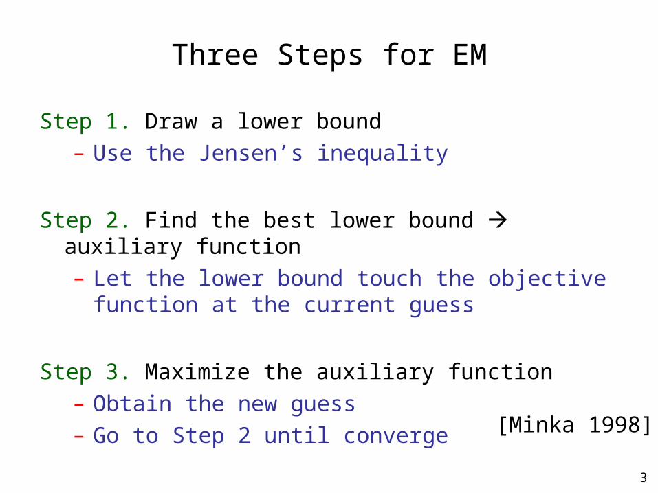
Three Steps for EM
Step 1. Draw a lower bound– Use the Jensen’s inequality
Step 2. Find the best lower bound auxiliary function– Let the lower bound touch the objective function at the
current guess
Step 3. Maximize the auxiliary function– Obtain the new guess– Go to Step 2 until converge
[Minka 1998]
4
)(F
objective function
current guess
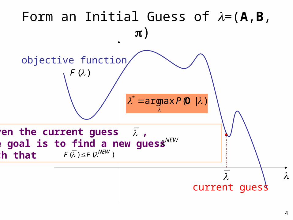
Form an Initial Guess of =(A,B,)
Given the current guess , the goal is to find a new guess such that
NEW
)()( NEWFF
)|(maxarg*
OP
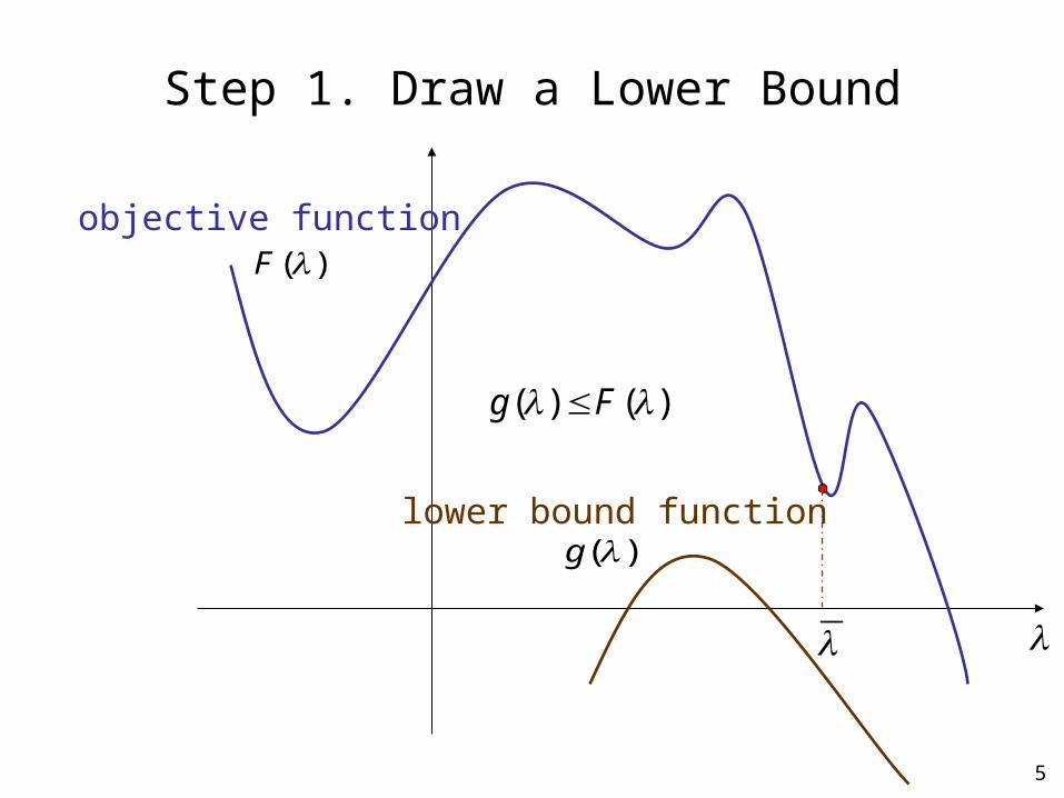
5
)(F
)()( Fg
Step 1. Draw a Lower Bound
)(glower bound function
objective function
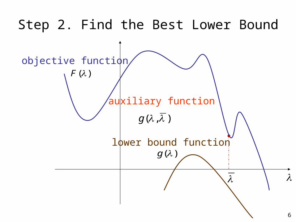
6
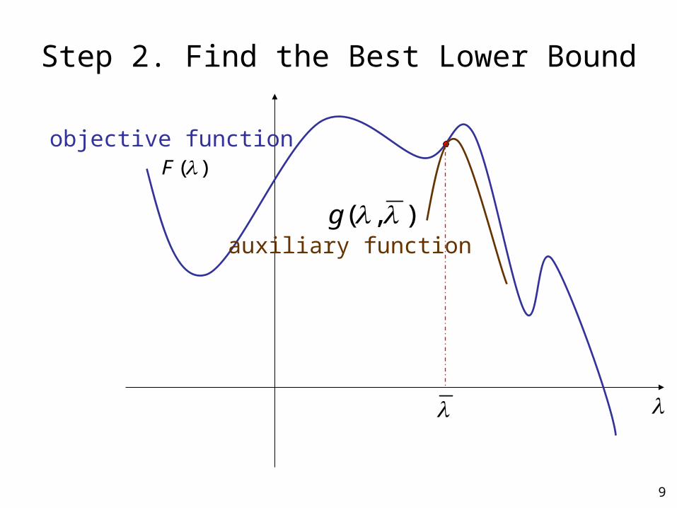
)(F
Step 2. Find the Best Lower Bound
objective function
lower bound function)(g
),( g
auxiliary function
7
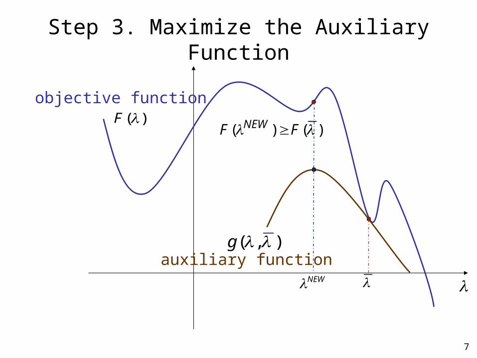
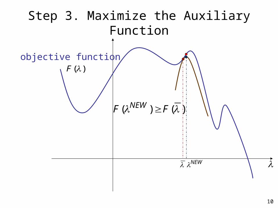
)(F
),( g
Step 3. Maximize the Auxiliary Function
NEW
)()( FF NEW
auxiliary function
objective function
8
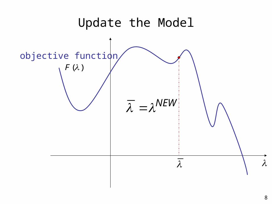
)(F
Update the Model
NEW
objective function
9
)(F
),( g
Step 2. Find the Best Lower Bound
objective function
auxiliary function
10
)(F
NEW
Step 3. Maximize the Auxiliary Function
)()( FF NEW
objective function
11
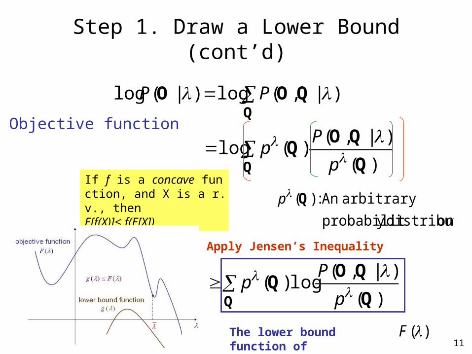
Step 1. Draw a Lower Bound (cont’d)
Q
Q
Q
QOQ
QOO
)(
)|,()(log
)|,(log)|(log
p
Pp
PP
Apply Jensen’s Inequality
The lower bound function of
)(F
ondistributiy probabilit
arbitrary An : )(QpIf f is a concave function, and X is a r.v., thenE[f(X)]≤ f(E[X])
Q Q
QOQ
)(
)|,(log)(
p
Pp
Objective function
12
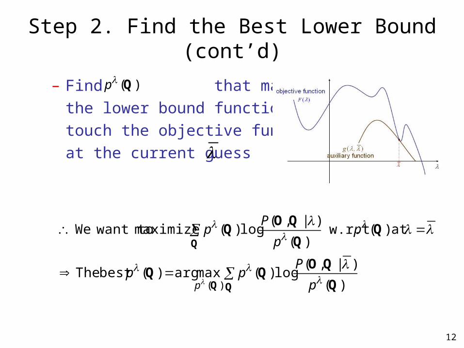
Step 2. Find the Best Lower Bound (cont’d)
– Find that makes
the lower bound function
touch the objective function
at the current guess
Q
Q
QOQQ
QOQ
)(
)|,(log)(maxarg)(best The
at )( w.r.t )(
)|,(log)( maximize want to We
)(
p
Ppp
pp
Pp
p
)(Qp
13
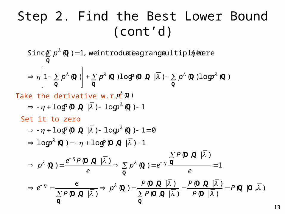
Step 2. Find the Best Lower Bound (cont’d)
),|()|(
)|,(
)|,(
)|,()(
)|,(
1
)|,(
)()|,(
)(
1)|,(log)(log
01)(log)|,(log
1)(log)|,(log
)(log)()|,(log)()(1
here multiplier Lagrange a introduce we,1)( Since
OQO
QO
QO
QOQ
QO
QO
QQO
Q
QOQ
QQO
QQO
QQQOQQ
Q
Q
Q
QQQ
Q
PP
P
P
Pp
P
ee
e
P
epe
Pep
Pp
pP
pP
ppPpp
p
Take the derivative w.r.t )(Qp
Set it to zero
14
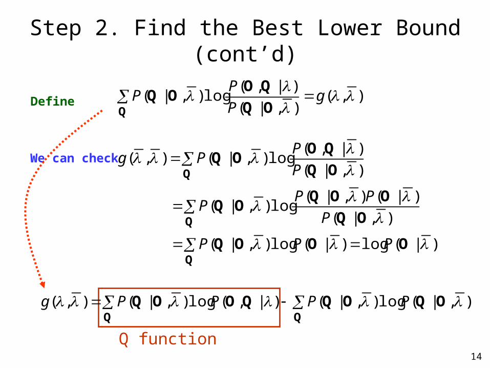
Step 2. Find the Best Lower Bound (cont’d)
Q function
)|(log)|(log),|(
),|(
)|(),|(log),|(
),|(
)|,(log),|(),(
OOOQ
OQ
OOQOQ
OQ
QOOQ
Q
Q
Q
PPP
P
PPP
P
PPg
We can check
),(),|(
)|,(log),|(
g
P
PP
Q OQ
QOOQDefine
OQOQQOOQ ),|(log),|()|,(log),|(),( PPPPg
15
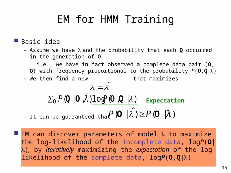
EM for HMM Training
Basic idea– Assume we have and the probability that each Q occurred in the
generation of O
i.e., we have in fact observed a complete data pair (O,Q) with frequency proportional to the probability P(O,Q|)
– We then find a new that maximizes
– It can be guaranteed that
EM can discover parameters of model to maximize the log-likelihood of the incomplete data, logP(O|), by iteratively maximizing the expectation of the log-likelihood of the complete data, logP(O,Q|)
Q QOOQ )|,(log),|( PλP ˆ
)|()ˆ|( λPP OO Expectation
16
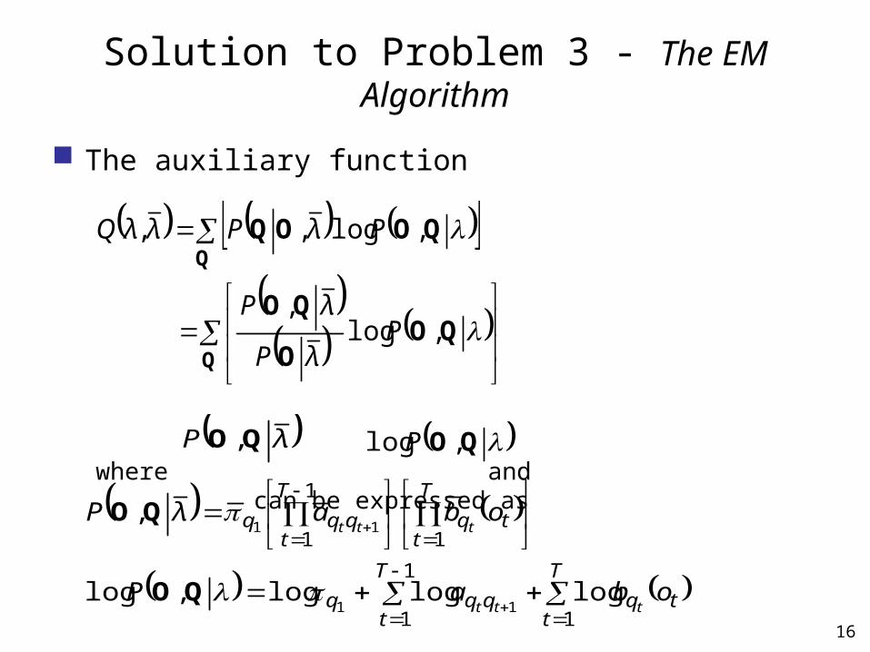
Solution to Problem 3 - The EM Algorithm
The auxiliary function
where and can be expressed as
Q
Q
QOO
QO
QOOQ
,log,
,log,,
PλP
λP
PλPλλQ
T
ttq
T
tqqq
T
ttq
T
tqqq
obaP
obaλP
ttt
ttt
1
1
1
1
1
1
logloglog,log
,
11
11
QO
QO
λP QO, QO,log P
17
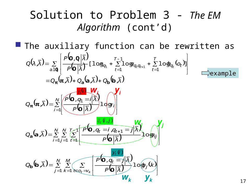
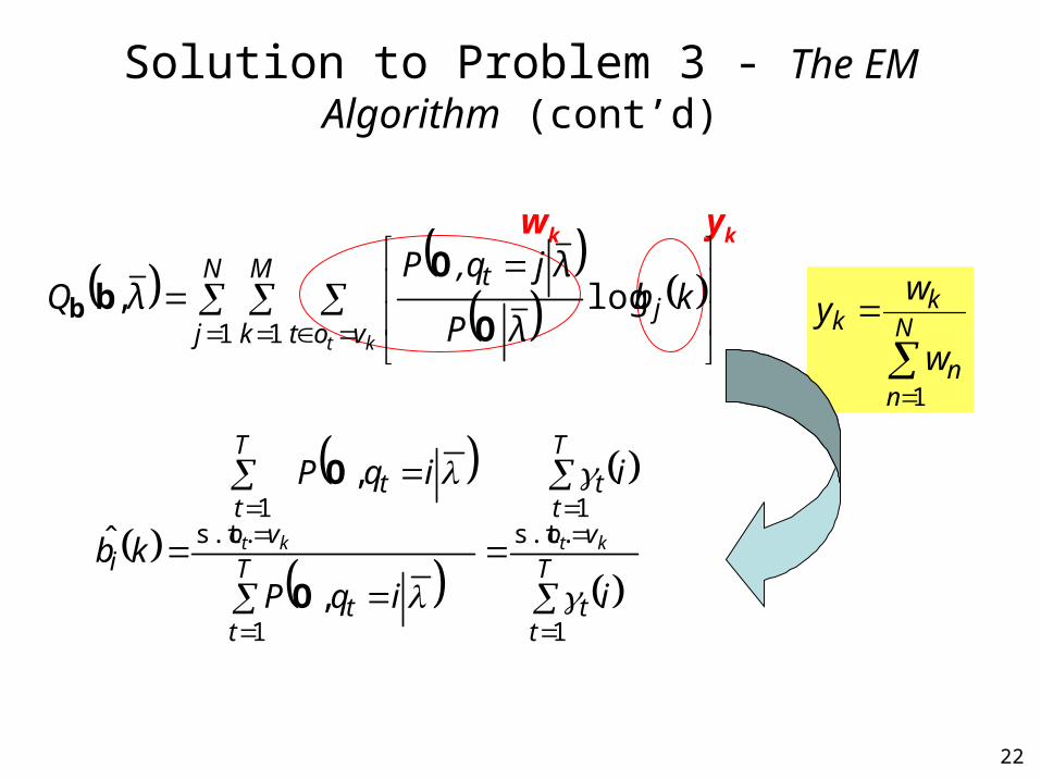
Solution to Problem 3 - The EM Algorithm (cont’d)
The auxiliary function can be rewritten as
wi yi
wj yj
wk yk
N
j
M
k votj
t
N
i
N
j
T
tij
tt
N
ii
kt
kbλP
λj,qPλQ
aλP
λjqi,qPλQ
λP
λi,qPλQ
1 1
1 1
1
1
1
1
1
log,
log,
,
log,
O
Ob
O
Oa
O
Oπ
b
a
π
i1
)(it
),( jit
λQλQλQ
obaλP
λ,PλλQ
T
ttq
T
tqqq ttt
,,,
]loglog[log, all 1
1
111
baπ
O
QO
baπ
Q
example
18
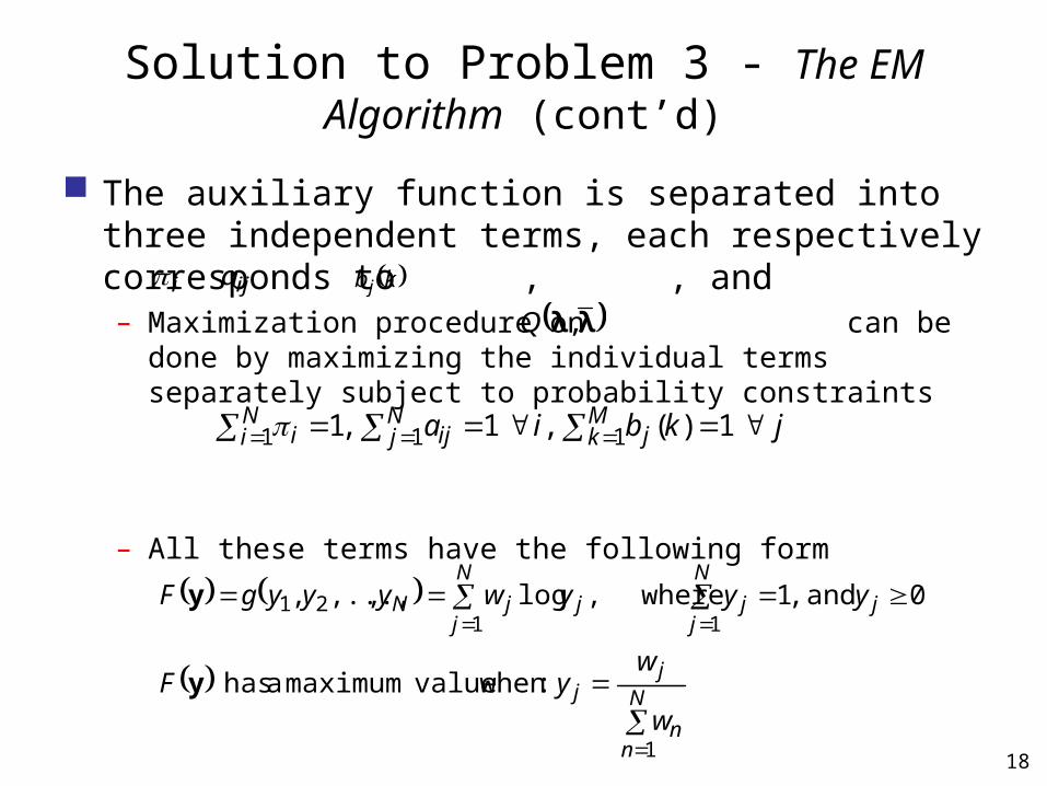
Solution to Problem 3 - The EM Algorithm (cont’d)
The auxiliary function is separated into three independent terms, each respectively corresponds to , , and – Maximization procedure on can be done by maximizing
the individual terms separately subject to probability constraints
– All these terms have the following form
ija kb ji
N
nn
jj
j
N
jj
N
jjjN
w
wyF
yyywyyygF
1
1121
: when valuemaximum a has
0 and ,1 where,log,,...,,
y
y
Mk j
Nj ij
Ni i jkbia 111 1)( , 1 ,1
λλ,Q

19
Solution to Problem 3 - The EM Algorithm (cont’d)
Proof: Apply Lagrange Multiplier
N
nn
jj
N
jj
N
jj
N
jj
N
jj
j
j
j
j
j
N
j
N
jjjj
N
jjj
w
wy
wwyy
jy
w
y
w
y
F
yywywF
1
1111
1 11
0Then
0 Letting
1loglog that Suppose
Multiplier Lagrange applyingBy
Constraint
xe
xxh
x
xhxh
h
xhx
h
xhx
dx
xd
he
hx
xh
xhx
h
h
h
hh
h
h
1ln
1/1lnlim
1
/1lnlim/1lnlim
/lnlim
)ln()ln(lim
ln
...71828.21lim
/
0/
/1/
0
/1
0
00
/1
0
20
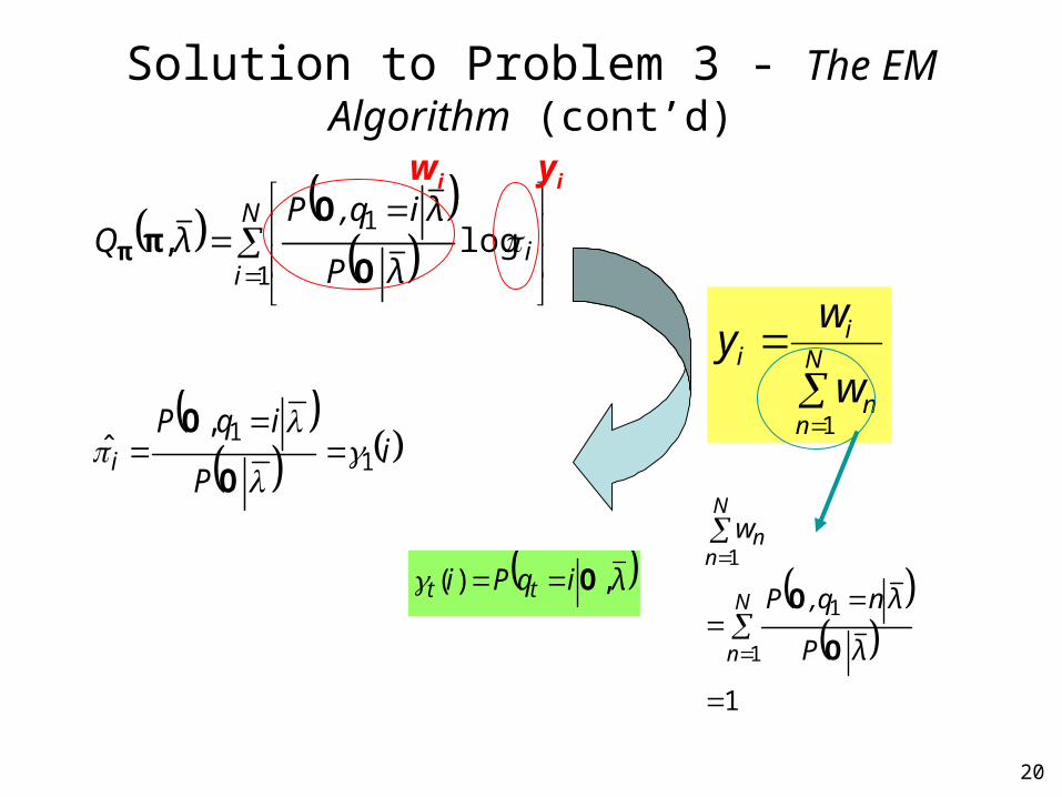
Solution to Problem 3 - The EM Algorithm (cont’d)
N
ii
λP
λi,qPλQ
1
1log,
O
Oππ
wi yi
N
nn
ii
w
wy
1 i
P
iqPi 1
1,ˆ
O
O
λiqPi tt ,)( O
1
1
1
1
N
n
N
nn
λP
λn,qP
w
O
O
21
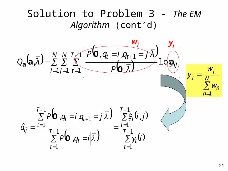
Solution to Problem 3 - The EM Algorithm (cont’d)
N
nn
jj
w
wy
1
1
1
1
11
1
1
11 ,
,
,,ˆ
T
tt
T
tt
T
tt
T
ttt
ij
i
ji
iqP
jqiqPa
O
O
N
i
N
j
T
tij
tta
λP
λjqi,qPλQ
1 1
1
1
1log
,,
O
Oaa
wj yj
22
Solution to Problem 3 - The EM Algorithm (cont’d)
N
nn
kk
w
wy
1
wk yk
T
tt
T
vot
t
T
tt
T
vot
t
i
i
i
iqP
iqP
kb ktkt
1
s.t.1
1
s.t.1
,
,
ˆ
O
O
N
j
M
k votj
t
kt
kbλP
λj,qPλQ
1 1log,
O
Obb
23
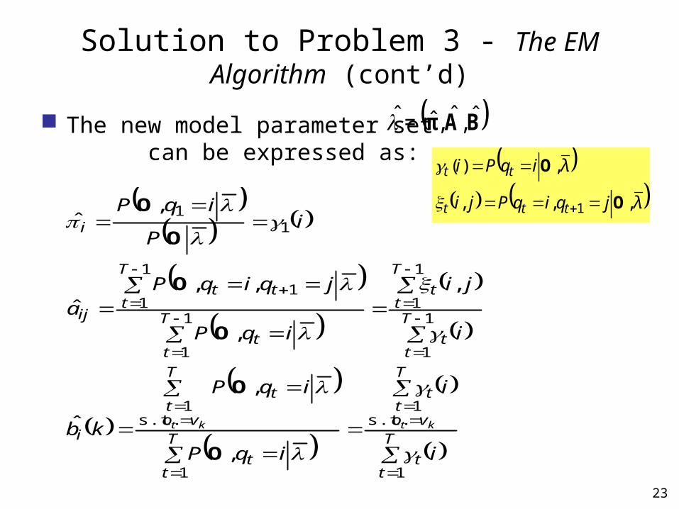
Solution to Problem 3 - The EM Algorithm (cont’d)
The new model parameter set can be expressed as:
BAπ ˆ,ˆ,ˆ=̂
T
tt
T
vot
t
T
tt
T
vot
t
i
T
tt
T
tt
T
tt
T
ttt
ij
i
i
i
iqP
iqP
kb
i
ji
iqP
jqiqPa
iP
iqP
ktkt
1
s.t.1
1
s.t.1
1
1
1
11
1
1
11
11
,
,
ˆ
,
,
,,ˆ
,ˆ
O
O
O
O
O
O
λjqiqPji
λiqPi
ttt
tt
,,,
,)(
1 O
O
24
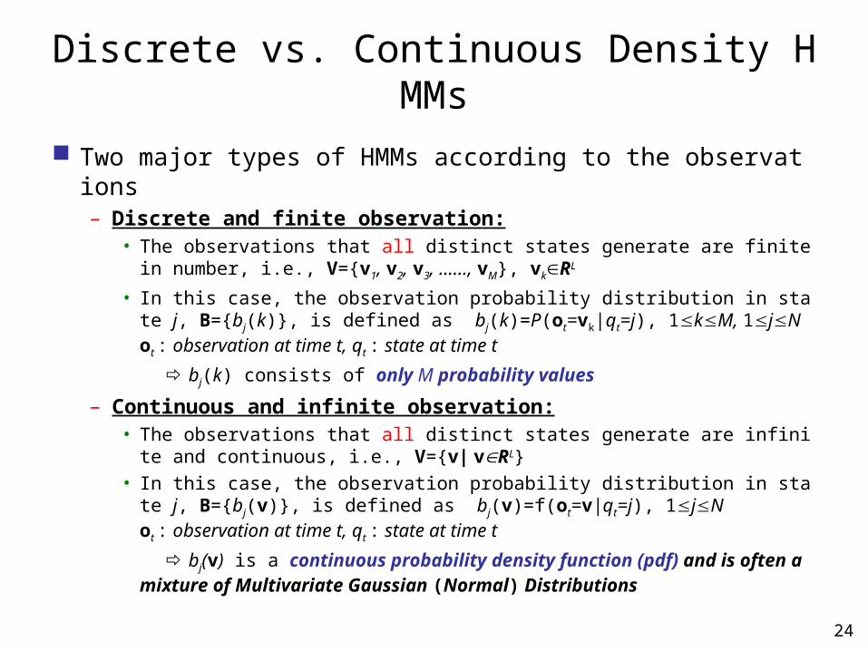
Discrete vs. Continuous Density HMMs
Two major types of HMMs according to the observations– Discrete and finite observation:
• The observations that all distinct states generate are finite in number, i.e., V={v1, v2, v3, ……, vM}, vkRL
• In this case, the observation probability distribution in state j, B={bj(k)}, is defined as bj(k)=P(ot=vk|qt=j), 1kM, 1jNot : observation at time t, qt : state at time t
bj(k) consists of only M probability values
– Continuous and infinite observation:• The observations that all distinct states generate are infinite and contin
uous, i.e., V={v| vRL}
• In this case, the observation probability distribution in state j, B={bj(v)}, is defined as bj(v)=f(ot=v|qt=j), 1jNot : observation at time t, qt : state at time t
bj(v) is a continuous probability density function (pdf) and is often a mixture of Multivariate Gaussian (Normal) Distributions
25
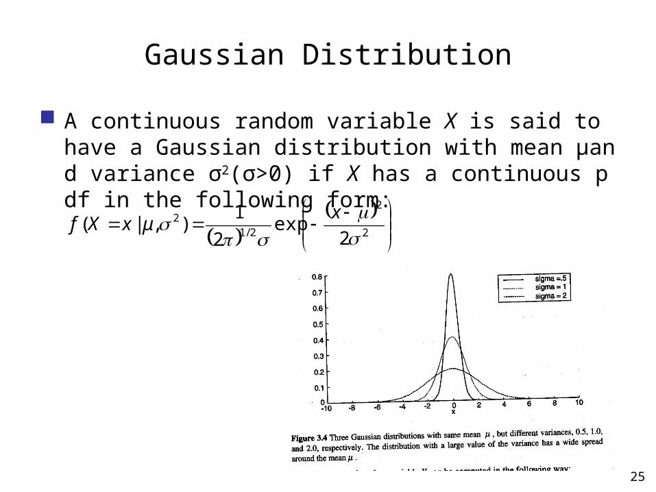
Gaussian Distribution
A continuous random variable X is said to have a Gaussian distribution with mean μand variance σ2(σ>0) if X has a continuous pdf in the following form:
2
2
2/12
2exp
2
1),|(
x
μxXf
26
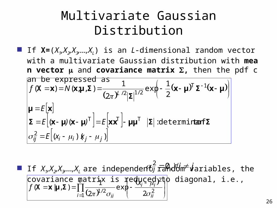
Multivariate Gaussian Distribution
If X=(X1,X2,X3,…,XL) is an L-dimensional random vector with a multivariate Gaussian distribution with mean vector and covariance matrix , then the pdf can be expressed as
If X1,X2,X3,…,XL are independent random variables, the covariance matrix is reduced to diagonal, i.e.,
))((
oft determinan : ((
2
1exp
2
1),;()(
2
TTT
1T2/12/
jjiiij
L
xxE
E))E
E
Nf
ΣΣμμxxμxμxΣ
xμ
μxΣμxΣ
ΣμxxX
jiij ,02
L
i ii
ii
ii
xf
12
2
2/1 2exp
2
1),|(
ΣμxX
27
Multivariate Mixture Gaussian Distribution
An L-dimensional random vector X=(X1,X2,X3,…,XL) is with a multivariate mixture Gaussian distribution if
In CDHMM, bj(v) is a continuous probability density function (pdf) and is often a mixture of multivariate Gaussian distributions
M
kjkjkjk
jkL
jkj cb1
1T2/12/ 2
1exp
2
1μvΣμv
Σv
M
kjkjk cc
1
1and0 Covariance matrix of the kth mixture of the jth state
Mean vectorof the kth mixture of the jth state
Observation vector
wNwfM
kk
M
kkkk 1 ,),;()(
11
Σμxx
28
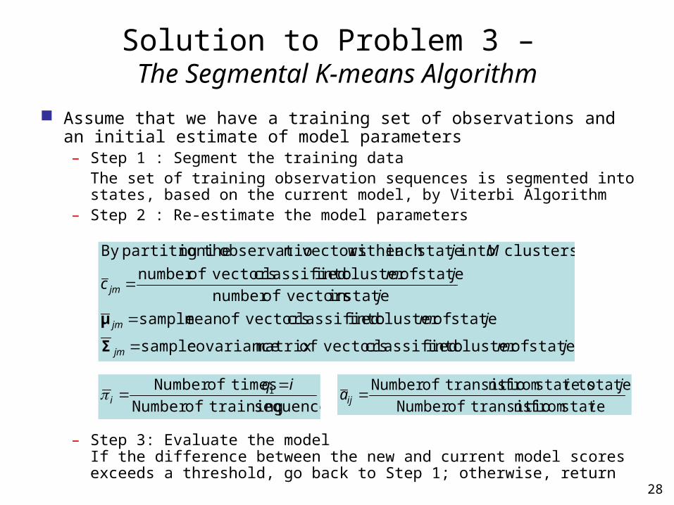
Solution to Problem 3 – The Segmental K-means Algorithm
Assume that we have a training set of observations and an initial estimate of model parameters– Step 1 : Segment the training data
The set of training observation sequences is segmented into states, based on the current model, by Viterbi Algorithm
– Step 2 : Re-estimate the model parameters
– Step 3: Evaluate the model If the difference between the new and current model scores exceeds a threshold, go back to Step 1; otherwise, return
sequences trainingofNumber
timesofNumber 1 iqi
state from ns transitioofNumber
state to state from ns transitioofNumber
i
jiaij
state of cluster into classified vectorsofmatrix covariance sample
state of cluster into classified vectorsofmean sample
statein vectorsofnumber
state of cluster into classified vectorsofnumber
clusters into stateeach within n vectorsobservatio thengpartitioniBy
jm
jm
j
jmc
Mj
jm
jm
jm
Σ
μ
29
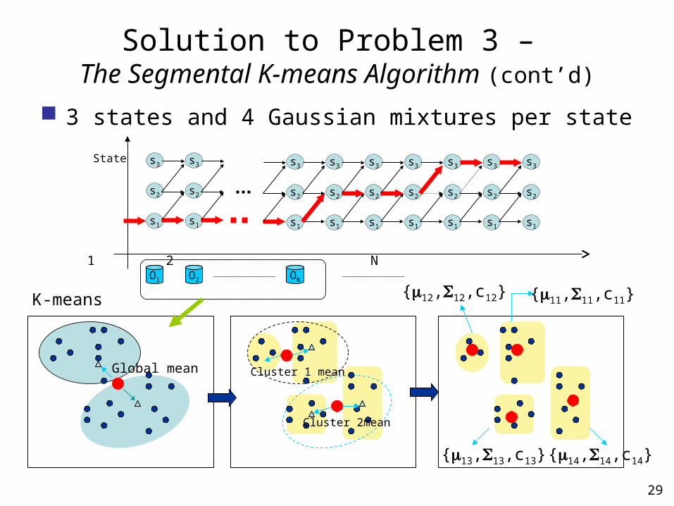
Solution to Problem 3 – The Segmental K-means Algorithm (cont’d)
3 states and 4 Gaussian mixtures per state
O1
State
O2
1 2 NON
s2
s3
s1
s2
s3
s1
s2
s3
s1
s2
s3
s1
s2
s3
s1
s2
s3
s1
s2
s3
s1
s2
s3
s1
s2
s3
s1
Global mean Cluster 1 mean
Cluster 2mean
K-means {11,11,c11}{12,12,c12}
{13,13,c13} {14,14,c14}
30
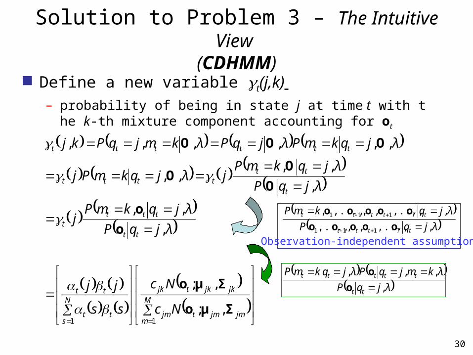
Solution to Problem 3 – The Intuitive View (CDHMM)
Define a new variable t(j,k) – probability of being in state j at time t with the k-th mixture com
ponent accounting for ot
M
mjmjmtjm
jkjktjk
N
stt
tt
tt
tttt
t
tttttt
tttttt
Nc
Nc
ss
jj
λjqP
λjqkmPj
λjqP
λjqkmPjλjqkmPj
λjqkmPλjqPλkmjqPkj
11,;
,;
,
,,
,
,,,,
,,,,,,
Σμo
Σμo
o
o
O
OO
OOO
Observation-independent assumption
λjqP
λjqkmP
tTttt
tTtttt
,,...,,,,...,
,,...,,,,...,,
111
111
ooooo
ooooo
λjqP
λkmjqPλjqkmP
tt
ttttt
,
,,,
o
o
31
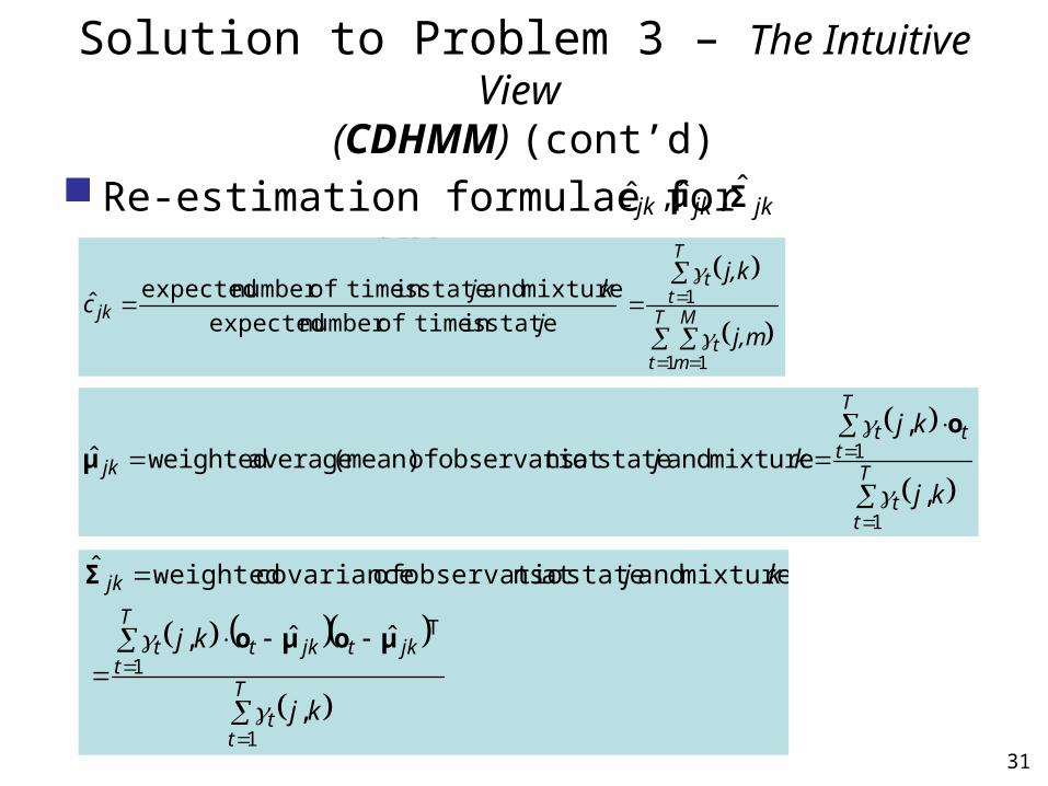
Solution to Problem 3 – The Intuitive View (CDHMM) (cont’d)
Re-estimation formulae for are
T
tt
T
ttt
jk
kj
kjkj
1
1
,
, mixture and stateat nsobservatio of (mean) average weightedˆ
oμ
j,m
j,k
j
kjc
T
t
M
mt
T
tt
jk
1 1
1 statein timesofnumber expected
mixture and statein timesofnumber expectedˆ
T
tt
T
tjktjktt
jk
kj
kj
kj
1
1
T
,
ˆˆ,
mixture and stateat nsobservatio of covariance weightedˆ
μoμo
Σ
jkjkjkc Σμ ˆ ,ˆ ,ˆ
32
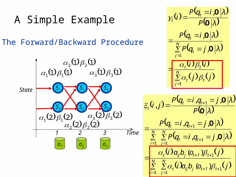
A Simple Example
o1
State
o2 o3
1 2 3 Time
S1
S2
S1
S2
S1
S2
1 1 11
2 2 11 2 2 22
2 2 33
1 1 22 1 1 33
The Forward/Backward Procedure
N
jtt
tt
N
jt
t
tt
jj
ii
λjqP
λiqP
λP
λiqPi
1
1
,
,
,
O
O
O
O
N
jt1tjijt
N
i
t1tjijt
N
jtt
N
i
tt
ttt
jobai
jobai
λjqiqP
λjqiqP
λP
λjqiqPji
11
1
1
11
1
1
1
)(
)(
,,
,,
,,,
O
O
O
O
33
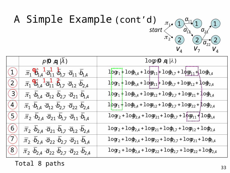
A Simple Example (cont’d) 1
2
1
2
1
2
4v 7v 4v
start1
2
11a
12a
22a
21a
4,1117,1114,11 babab 1 4,1117,1114,11 loglogloglogloglog babab
4,2127,1114,11 babab 2 4,2127,1114,11 loglogloglogloglog babab
4,1217,2124,11 babab 3 4,1217,2124,11 loglogloglogloglog babab
4,2227,2124,11 babab 4 4,2227,2124,11 loglogloglogloglog babab
4,1117,1214,22 babab 5 4,1117,1214,22 loglogloglogloglog babab
4,2127,1214,22 babab 6 4,2127,1214,22 loglogloglogloglog babab
4,1217,2224,22 babab 7 4,1217,2224,22 loglogloglogloglog babab
4,2227,2224,22 babab 8 4,2227,2224,22 loglogloglogloglog babab
)|,(log qOp)|,( λp qO
Total 8 paths
q: 1 1 1
q: 1 1 2
34
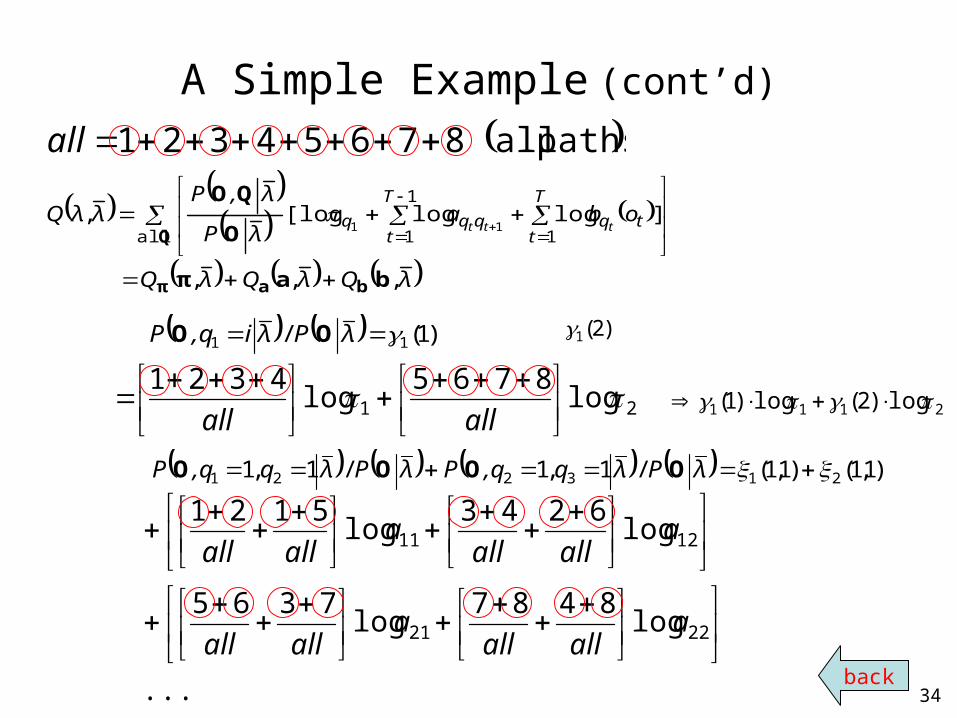
A Simple Example (cont’d)
pathsall 87654321 all
21 log8765
log4321
allall
...
log8487
log7365
log6243
log5121
2221
1211
aallall
aallall
aallall
aallall
back
)1,1()1,1(/1,1/1,1 213221 λPλq,qPλPλq,qP OOOO
λQλQλQ
obaλP
λ,PλλQ
T
ttq
T
tqqq ttt
,,,
]loglog[log, all 1
1
111
baπ
O
QO
baπ
Q
2111 log)2(log)1(
)1(/ 11 λPλi,qP OO )2(1


![SVM-HMM LANDMARK BASED SPEECH RECOGNITIONsborys/borys08.pdf · as their integration with an HMM back end. Part of this work has previously been reported in [58,59]. 2 Background In](https://static.fdocuments.in/doc/165x107/5f0a0e6e7e708231d429cdcc/svm-hmm-landmark-based-speech-sborysborys08pdf-as-their-integration-with-an.jpg)


