HJM Model for Interest Rates and Credit - MIT … 24 HJM Model for Interest Rates and Credit Denis...

Lecture 24

HJM Model for Interest Rates and Credit

Denis Gorokhov

(Executive Director, Morgan Stanley)

Developed for educational use at MIT and for publication through MIT OpenCourseware.

No investment decisions should be made in reliance on this material.

Only Source /

Footnotes below this

line

Guid

e @

4.6

9

2 2

Denis Gorokhov Denis Gorokhov is an Executive Director at Morgan Stanley. During his

9 years at the firm Mr. Gorokhov worked on pricing exotic derivatives with emphasis on credit, counterparty risk, asset-backed securities, inflation, and longevity.

Mr. Gorokhov obtained a number of original analytic results for fixed income pricing problems which are implemented in Morgan Stanley risk management systems. He created a flexible modeling framework used for pricing over 400 different types of exotic derivatives including key transactions in the recent Morgan Stanley history: TARP transaction with US Treasury, purchase of 20% stake in Morgan Stanley by Mitsubishi UFJ Securities, and credit valuation adjustment with monoline insurer MBIA.

Prior to joining Morgan Stanley Mr. Gorokhov worked in the fields of superconductivity and mesoscopic physics and authored 20 papers in leading physics journals. Mr. Gorokhov holds a Ph.D. degree in theoretical physics from ETH-Zurich and spent several years as a post-doctoral researcher at Harvard and Cornell.

Mr. Gorokhov’s comments today are his own, and do not necessarily represent the views of Morgan Stanley or its affiliates, and are not a product of Morgan Stanley Research.



Only Source /


line

Guide @ 2.68

Guide @ 1.64

Guide @ 1.95

Subtitle Guide @ 2.64

Guide @ 2.80

Only Source / Footnotes below this line

Guide @ 0.22

Guid

e @

4.6

9

3

Introduction

HJM (Heath-Jarrow-Morton) model is a very general framework used for

pricing interest rates and credit derivatives.

Big banks trade hundreds, sometimes even thousands, of different types of

derivatives and need to have a modeling/technological framework which can

quickly accommodate new payoffs.

Compare this problem to that in physics. It is relatively straightforward to

solve Schrodinger equation for the hydrogen atom and find energy levels.

But what about energy spectra of complicated molecules or crystals?

Physicists use advanced computational methods in this case, e.g. LDA (local

density approximation).

Similarly, in the world of financial derivatives there is a very general

framework, Monte Carlo simulation, which in principle can be used for

pricing any financial contract.

The HJM model naturally fits into this concept.

Before discussing the HJM model it is very important to understand how the

Monte Carlo method appears in finance. Stock options are the best

example.



Only Source /


line

Guide @ 2.68

Guide @ 1.64

Guide @ 1.95


Guide @ 2.80


Guide @ 0.22

Guid

e @

4.6

9

4

Dynamic Hedging

Dealers are trying to match buy and sell orders from clients. It is not always

possible and they have to hedge the residual positions.

In the example below a dealer sold a call option on a stock, the loss may be

unlimited. To hedge the exposure the dealer takes a position in an

underlying and adjusts it dynamically.

Stock price

Payoff

0

Premium

Strike



Only Source /


line

Guide @ 2.68

Guide @ 1.64

Guide @ 1.95


Guide @ 2.80


Guide @ 0.22

Guid

e @

4.6

9

5

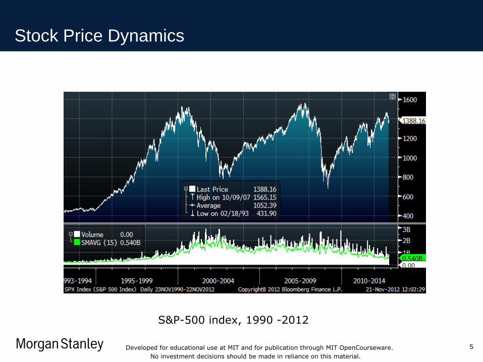
Stock Price Dynamics

S&P-500 index, 1990 -2012



Only Source /


line

Guide @ 2.68

Guide @ 1.64

Guide @ 1.95


Guide @ 2.80


Guide @ 0.22

Guid

e @

4.6

9

6

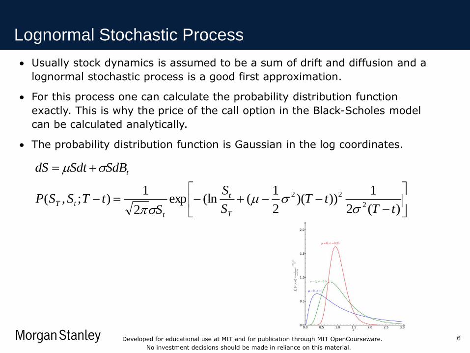
Lognormal Stochastic Process

)(2

1)))(

2

1((lnexp

2

1);,(

2

22

tTtT

S

S

StTSSP

SdBSdtdS

T

t

t

tT

t

Usually stock dynamics is assumed to be a sum of drift and diffusion and a

lognormal stochastic process is a good first approximation.

For this process one can calculate the probability distribution function

exactly. This is why the price of the call option in the Black-Scholes model

can be calculated analytically.

The probability distribution function is Gaussian in the log coordinates.



//upload.wikimedia.org/wikipedia/commons/8/80/Some_log-normal_distributions.svg

Only Source /


line

Guide @ 2.68

Guide @ 1.64

Guide @ 1.95


Guide @ 2.80


Guide @ 0.22

Guid

e @

4.6

9

7

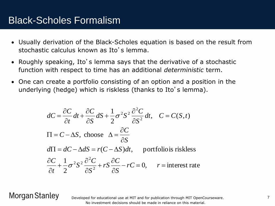
Black-Scholes Formalism

rateinterest ,02

1

riskless is portfolio ,)(

choose ,

),( ,2

1

2

222

2

222

rrCS

CrS

S

CS

t

C

dtSCrdSdCd

S

CSC

tSCCdtS

CSdS

S

Cdt

t

CdC

Usually derivation of the Black-Scholes equation is based on the result from

stochastic calculus known as Ito’s lemma.

Roughly speaking, Ito’s lemma says that the derivative of a stochastic

function with respect to time has an additional deterministic term.

One can create a portfolio consisting of an option and a position in the

underlying (hedge) which is riskless (thanks to Ito’s lemma).



Only Source /


line

Guide @ 2.68

Guide @ 1.64

Guide @ 1.95


Guide @ 2.80


Guide @ 0.22

Guid

e @

4.6

9

8

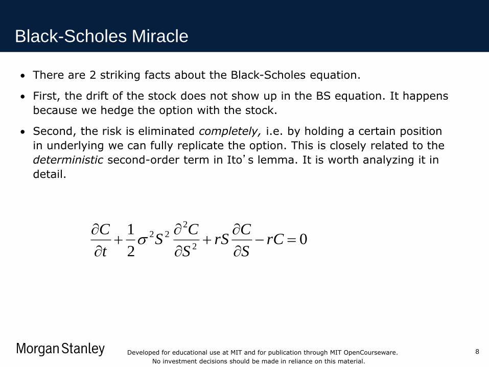
Black-Scholes Miracle

There are 2 striking facts about the Black-Scholes equation.

First, the drift of the stock does not show up in the BS equation. It happens

because we hedge the option with the stock.

Second, the risk is eliminated completely, i.e. by holding a certain position

in underlying we can fully replicate the option. This is closely related to the

deterministic second-order term in Ito’s lemma. It is worth analyzing it in

detail.

02

12

222

rC

S

CrS

S

CS

t

C



Only Source /


line

Guide @ 2.68

Guide @ 1.64


Guide @ 2.80


Guide @ 0.22

Guid

e @

4.6

9

9

Ito’s Lemma under Microscope

0 N N-1 … 1 i i-1 i+1

dt

dt’

'222

2

2

100

'222

2

2

1

'

11

2

12

2

1

'

11

''

1

2

1),(),(),(

2

1),(),(

,1...0 ,2

1),(),(

)1,0(~ ,

dtSS

CSStS

S

Cdt

t

CtSCtSC

dtSS

CSS

S

Cdt

t

CtSCtSC

NiSSS

CSS

S

Cdt

t

CtSCtSC

NdtSdtSSS

i

i

i

iiiiNN

iiiiiii

iiiiiiii

iiiiii

• In the limit N->infinity the sum in the last term of the last equation becomes deterministic and we obtain Ito’s lemma!



Only Source /


line

Guide @ 2.68

Guide @ 1.64

Guide @ 1.95


Guide @ 2.80


Guide @ 0.22

Guid

e @

4.6

9

10

Black-Scholes Miracle - 2

Exercise 1: Prove that )1,0(~ , i

1

2 NN

i

i

is deterministic in the limit N->infinity.

• Exercise 2: Look up a “proof” of Ito’s lemma in Hull’s book (J.C. Hull, Options, Futures, and Other Derivatives) and find an error (pages 232-233 in 5th edition).

We see that complete risk elimination in the Black-Scholes model is due to

the existence of 2 different time scales dt and dt’. One can derive the BS

equation in the limit dt->0, dt’->0, and dt/dt’->infinity.

From the business point of view this means that we hedge on a small time

scale dt’ and the profit/loss noise is finite, however as long as the time

interval increases to dt the profit/loss noise disappears!



Only Source /


line

Guide @ 2.68

Guide @ 1.64

Guide @ 1.95


Guide @ 2.80


Guide @ 0.22

Guid

e @

4.6

9

11

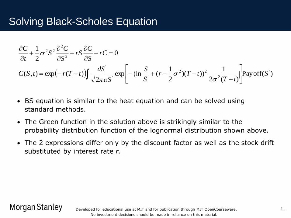
Solving Black-Scholes Equation

)(Payoff)(2

1)))(

2

1((lnexp

2)(exp),(

02

1

'

2

22

''

'

2

222

StT

tTrS

S

S

dStTrtSC

rCS

CrS

S

CS

t

C

BS equation is similar to the heat equation and can be solved using

standard methods.

The Green function in the solution above is strikingly similar to the

probability distribution function of the lognormal distribution shown above.

The 2 expressions differ only by the discount factor as well as the stock drift

substituted by interest rate r.



Only Source /


line

Guide @ 2.68

Guide @ 1.64

Guide @ 1.95


Guide @ 2.80


Guide @ 0.22

Guid

e @

4.6

9

12

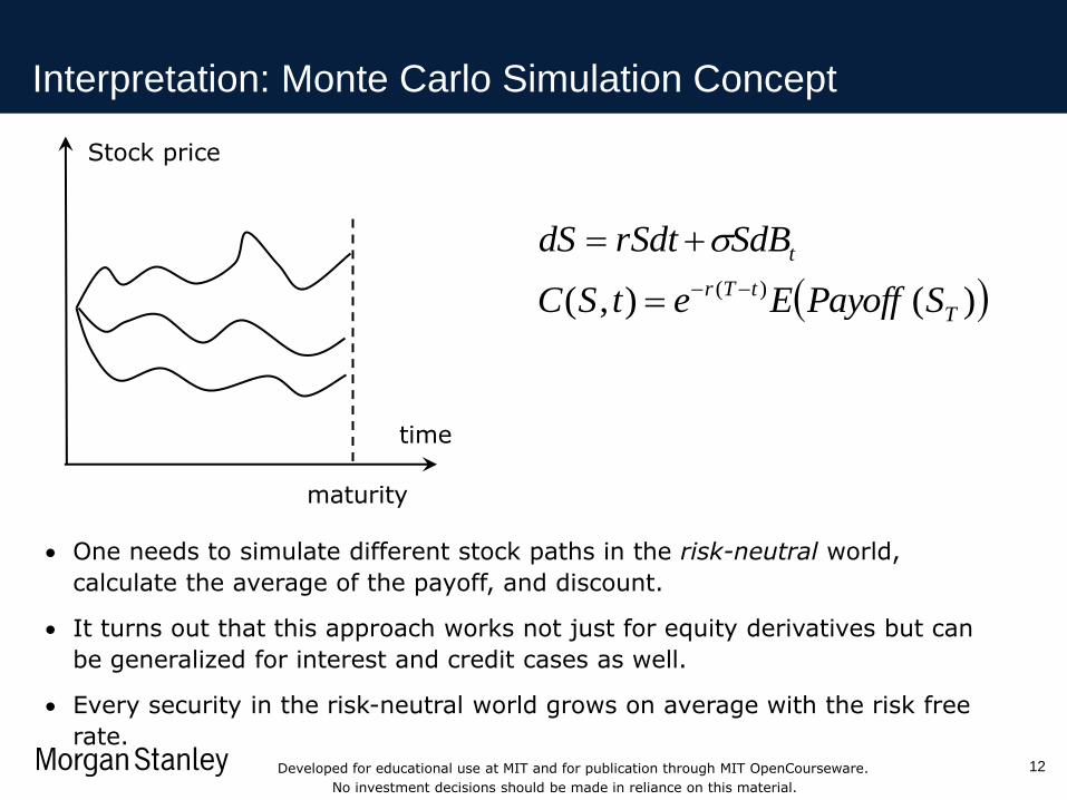
Interpretation: Monte Carlo Simulation Concept

time

Stock price

maturity

)(),( )(

T

tTr

t

SPayoffEetSC

SdBrSdtdS

One needs to simulate different stock paths in the risk-neutral world,

calculate the average of the payoff, and discount.

It turns out that this approach works not just for equity derivatives but can

be generalized for interest and credit cases as well.

Every security in the risk-neutral world grows on average with the risk free

rate.



Only Source /


line

Guide @ 2.68

Guide @ 1.64

Guide @ 1.95


Guide @ 2.80


Guide @ 0.22

Guid

e @

4.6

9

Interest Rates Derivatives: Basic Concepts

13

Businesses borrow money to finance their activity.

As a compensation lenders charge borrowers certain interest.

Interest rates fluctuate with time and, similar to the equity case, there exists a

market of derivatives linked to the level of interest rates.

Time value of money: $1 to be paid in 1 year form now is worth less than $1

paid in 2 years form now. For example, if 1- and 2-year interest rates are both

equal to 5%, then one needs to invest $1/(1+0.05)= $0.95 today to obtain $1

in 1 year form now and $1/(1+0.05)^2=$0.90 to obtain $1 in 2 years form

now.

It is very convenient to describe time value of money using discount factors.

1.0

discount factor

time 0



Only Source /


line

Guide @ 2.68

Guide @ 1.64

Guide @ 1.95


Guide @ 2.80


Guide @ 0.22

Guid

e @

4.6

9

Forward Rates

It is very convenient to express discount factors using forward rates.

Mathematically, the relation between discount factors and forward rates can

be expresses as

T

t

dsstfTtd )),(exp(),(

forward rate

time



Only Source /


line

Guide @ 2.68

Guide @ 1.64

Guide @ 1.95


Guide @ 2.80


Guide @ 0.22

Guid

e @

4.6

9

Yield of 10-year US Treasury Note

Interest rates are extremely low at present.



Only Source /


line

Guide @ 2.68

Guide @ 1.64

Guide @ 1.95



Guide @ 0.22

Guid

e @

4.6

9

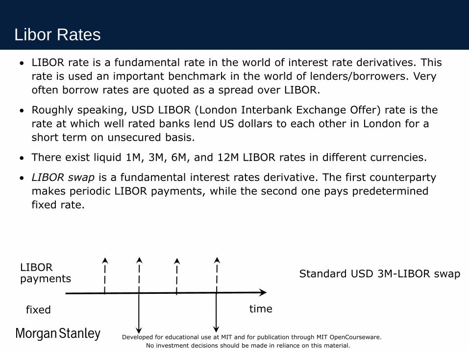
Libor Rates

LIBOR rate is a fundamental rate in the world of interest rate derivatives. This

rate is used an important benchmark in the world of lenders/borrowers. Very

often borrow rates are quoted as a spread over LIBOR.

Roughly speaking, USD LIBOR (London Interbank Exchange Offer) rate is the

rate at which well rated banks lend US dollars to each other in London for a

short term on unsecured basis.

There exist liquid 1M, 3M, 6M, and 12M LIBOR rates in different currencies.

LIBOR swap is a fundamental interest rates derivative. The first counterparty

makes periodic LIBOR payments, while the second one pays predetermined

fixed rate.

time

LIBOR payments

fixed

Standard USD 3M-LIBOR swap



Only Source /


line

Guide @ 2.68

Guide @ 1.64

Guide @ 1.95


Guide @ 2.80


Guide @ 0.22

Guid

e @

4.6

9

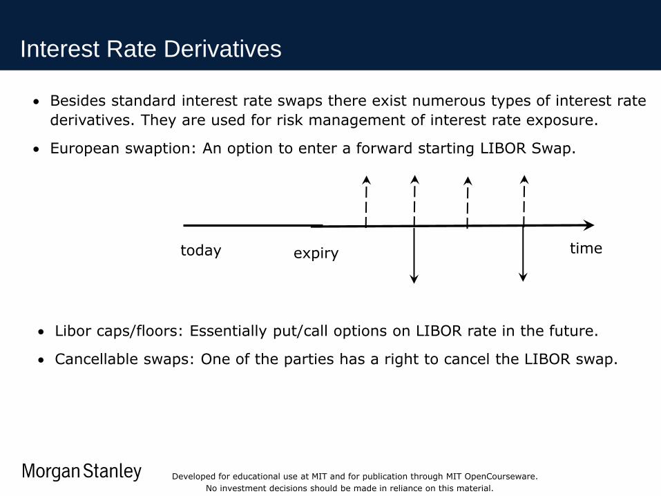
Interest Rate Derivatives

Besides standard interest rate swaps there exist numerous types of interest rate

derivatives. They are used for risk management of interest rate exposure.

European swaption: An option to enter a forward starting LIBOR Swap.

time today expiry

Libor caps/floors: Essentially put/call options on LIBOR rate in the future.

Cancellable swaps: One of the parties has a right to cancel the LIBOR swap.



Only Source /


line

Guide @ 2.68

Guide @ 1.64

Guide @ 1.95


Guide @ 2.80


Guide @ 0.22

Guid

e @

4.6

9

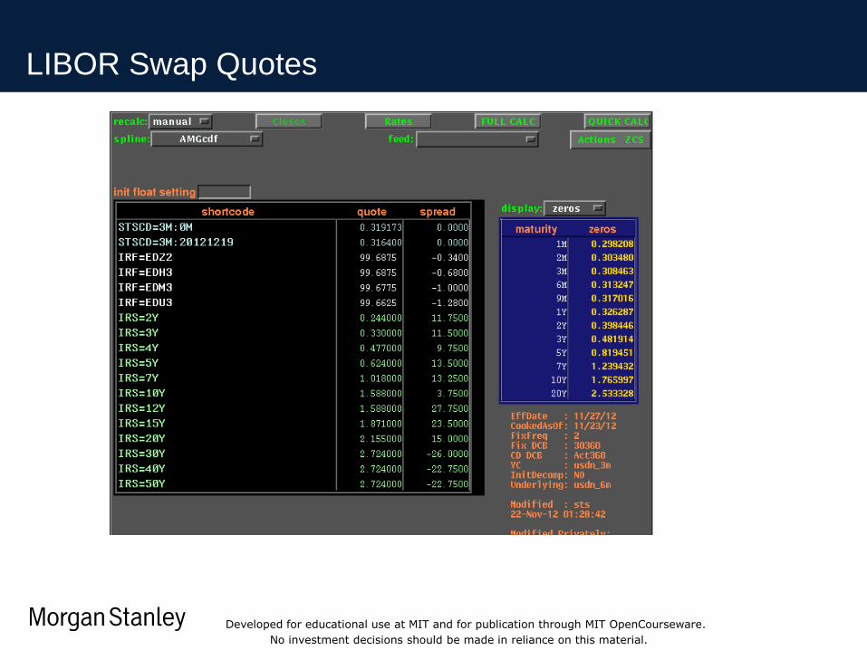
LIBOR Swap Quotes



Only Source /


line

Guide @ 2.68

Guide @ 1.64

Guide @ 1.95


Guide @ 2.80


Guide @ 0.22

Guid

e @

4.6

9

Pricing LIBOR Swaps, Discount Curve Cooking

)(tCdPV fixed

The LIBOR swap consists of 2 streams: fixed and floating ones. They can be

priced if we know the discount factor curve d=d(t).

The present value of a fixed payment C paid at time t is given by

There is a very neat result: present value of the float leg of a LIBOR swap plus a

notional payment at the end is equal to the notional. The PV of the swap

receiving fixed, paying float, and maturing at time T is

NTNdtcNdTPVi

i )()()(

But where from do we know the discount function d(t)? The swap market is very

liquid and we know swap rates corresponding to different maturities. One can

reverse engineer curve d(t) so that the observed swap rates are fair rates, i.e.

for all swaps PV(T)=0.

This procedure is know as discount curve bootstrapping (“cooking”).

Note: Here, we do not take into account OIS discounting.



Only Source /


line

Guide @ 2.68

Guide @ 1.64

Guide @ 1.95


Guide @ 2.80


Guide @ 0.22

Guid

e @

4.6

9

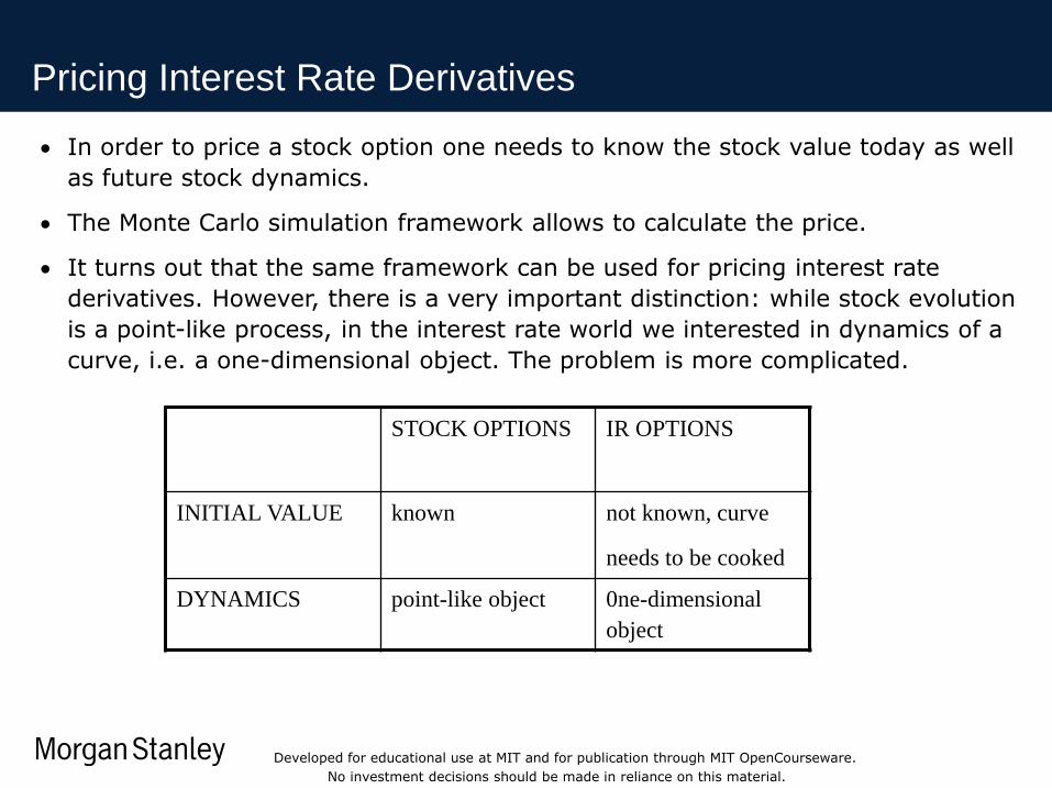
Pricing Interest Rate Derivatives

In order to price a stock option one needs to know the stock value today as well

as future stock dynamics.

The Monte Carlo simulation framework allows to calculate the price.

It turns out that the same framework can be used for pricing interest rate

derivatives. However, there is a very important distinction: while stock evolution

is a point-like process, in the interest rate world we interested in dynamics of a

curve, i.e. a one-dimensional object. The problem is more complicated.

STOCK OPTIONS IR OPTIONS

INITIAL VALUE known not known, curve

needs to be cooked

DYNAMICS point-like object 0ne-dimensional

object



Only Source /


line

Guide @ 2.68

Guide @ 1.64

Guide @ 1.95


Guide @ 2.80


Guide @ 0.22

Guid

e @

4.6

9

Classes of Interest Rates Models

Dynamic interest rates models can be divided into 2 large classes: term structure

models and short rate models.

The first class of models (more general) describes the dynamics of the full forward

curve, while the second class describes the short term rates only. Here is the list of

the most famous short rates models:

dBrdtrdr

dBdtrdr

dBdtdr

tttt

tttt

ttt

)(

)(

Ho-Lee model

Hull-White model

Cox-Ingersoll-Ross (CIR) model

• Note that the short rate and forward rates are related via

ttt fr



Only Source /


line

Guide @ 2.68

Guide @ 1.64

Guide @ 1.95


Guide @ 2.80


Guide @ 0.22

Guid

e @

4.6

9

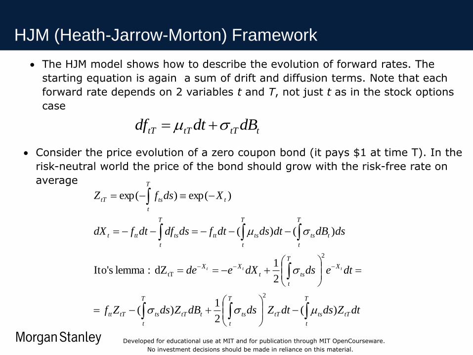
HJM (Heath-Jarrow-Morton) Framework

ttTtTtT dBdtdf

The HJM model shows how to describe the evolution of forward rates. The

starting equation is again a sum of drift and diffusion terms. Note that each

forward rate depends on 2 variables t and T, not just t as in the stock options

case

Consider the price evolution of a zero coupon bond (it pays $1 at time T). In the

risk-neutral world the price of the bond should grow with the risk-free rate on

average

dtZdsdtZdsdBZdsZf

dtedsdXede

dsdBdtdsdtfdsdfdtfdX

XdsfZ

tT

T

t

tstT

T

t

tsttT

T

t

tstTtt

X

T

t

tst

XX

t

T

t

ts

T

t

tstt

T

t

tsttt

t

T

t

tstT

ttt

)(2

1)(

2

1dZ :lemma sIto'

)()(

)exp()exp(

2

2

tT



Only Source /


line

Guide @ 2.68

Guide @ 1.64

Guide @ 1.95


Guide @ 2.80


Guide @ 0.22

Guid

e @

4.6

9

HJM Framework - 2

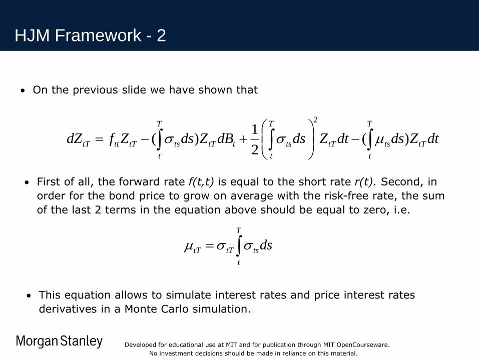
On the previous slide we have shown that

dtZdsdtZdsdBZdsZfdZ tT

T

t

tstT

T

t

tsttT

T

t

tstTtttT )(2

1)(

2

First of all, the forward rate f(t,t) is equal to the short rate r(t). Second, in

order for the bond price to grow on average with the risk-free rate, the sum

of the last 2 terms in the equation above should be equal to zero, i.e.

ds

T

t

tstTtT

This equation allows to simulate interest rates and price interest rates

derivatives in a Monte Carlo simulation.



Only Source /


line

Guide @ 2.68

Guide @ 1.64

Guide @ 1.95


Guide @ 2.80


Guide @ 0.22

Guid

e @

4.6

9

HJM Model Summary: How to Price IR Derivatives

ttT

T

t

tstTtT dBdtdsdf

Take IR swap quotes and bootstrap the discount curve.

Obtain forward rates from the discount curve. This is the starting point of the

simulation.

Specify the volatility of forward rates.

If the volatility is known, the drift can be calculated.

Start the simulation, stop at maturity, and price the derivative value by

averaging and discounting, similar to the stock option case.

IR volatility can be calibrated from the swaptions market.

initial curve f(0,T)

simulated curves at maturity

)(0 tPayoffeEPV

t

ssdsf

t



Only Source /


line

Guide @ 2.68

Guide @ 1.64

Guide @ 1.95


Guide @ 2.80


Guide @ 0.22

Guid

e @

4.6

9

Credit Derivatives: a Quick Introduction

When a borrower issues debt, there is a chance that money will not be returned.

This type of risk is known as credit risk and needs to be taken into account.

The higher the default risk for a particular issuer, the higher interest rate is

charged by the borrowers.

The interest rate can vary a lot among different issuers. For example, for 10-year

debt, the US government pays 1.7%/year (essentially, default-free rate), Morgan

Stanley pays around 5%/year, while the effective yield of bonds issued by

Greece is in the range 25-30%.

There exists a large credit derivatives market. The most important instrument is

credit default swap.

default swap buyer

default swap seller

periodic/upfront payments

payment upon default

In the event of default of a reference entity, seller pays the loss on a bond.



Only Source /


line

Guide @ 2.68

Guide @ 1.64

Guide @ 1.95


Guide @ 2.80


Guide @ 0.22

Guid

e @

4.6

9

Survival Probabilities and Hazard Rates

R

cp

pRNc

NpRcN

11

prob. survival recovery, notional, coupon,upfront

)1)(1(

It is very convenient to describe credit derivatives in terms of implied survival

probabilities. Let us illustrate this using a credit default swap example.

Assume that credit default swap protects against default on a bond with notional

N and recovery R. Assume for simplicity that interest rate is zero.

It is very convenient to parameterize survival probabilities with hazard rates.

Similar to the IR case on can write

T

t

dssthTtp )),(exp(),(



Only Source /


line

Guide @ 2.68

Guide @ 1.64

Guide @ 1.95


Guide @ 2.80


Guide @ 0.22

Guid

e @

4.6

9

Pricing Credit Derivatives

Remember that in the IR case one could price all derivatives using discount curve

d(t) whose meaning is the value of $1 paid at time t form now.

In the world of credit derivatives there is a notion of risky discount factors, i.e.

the value of $1 paid in the future subject to a possible default of a reference

entity.

Similar to the IR case one can “cook” survival probabilities from CDS market.

The present value of a CDS paying a loss on a bond can be written as follows

coupon running a ,)()1()()( 1 i

i

ii

i

ii dppNRtptaNdPV



Only Source /


line

Guide @ 2.68

Guide @ 1.64

Guide @ 1.95


Guide @ 2.80


Guide @ 0.22

Guid

e @

4.6

9

Dynamic Hazard Rate Model

In the case of credit default swaps pricing is relatively simple.

There are credit-linked instruments depending not only on survival probabilities

but also on their volatility, e.g. callable bonds.

Correct modeling of interest rate and credit dynamics allows to make optimal

call decisions.

Here is an example:

$14MM7years* $100MM*2% are savings

refinance, todecidedcompany the

3.0% spread effective 5.00% spread effective

1.50% spreadcredit 3.00% spreadcredit

1.50% rate freerisk 2.00% rate freerisk

changesmarket 3y thein bond $100MM10y a issues Xn corporatio



Only Source /


line

Guide @ 2.68

Guide @ 1.64

Guide @ 1.95


Guide @ 2.80


Guide @ 0.22

Guid

e @

4.6

9

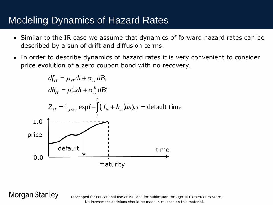
Modeling Dynamics of Hazard Rates

medefault ti),exp(1 }{

dshfZ

dBdtdh

dBdtdf

T

t

tststtT

h

t

h

tT

h

tTtT

ttTtTtT

Similar to the IR case we assume that dynamics of forward hazard rates can be

described by a sun of drift and diffusion terms.

In order to describe dynamics of hazard rates it is very convenient to consider

price evolution of a zero coupon bond with no recovery.

1.0

0.0 maturity

time

price

default



Only Source /


line

Guide @ 2.68

Guide @ 1.64

Guide @ 1.95


Guide @ 2.80


Guide @ 0.22

Guid

e @

4.6

9

Drift Condition for Hazard Rates

Exercise 3: Derive a drfit expression for the credit HJM model.

Hint: Consider dynamics of a zero coupon bond and average over the default

event. The resulting drift in this case should be equal to the risk-free rate. This

leads to a condition for the drift of forward hazard rates.

If there are no correlations between IR and hazard rates, the drift is given by the

equation similar to the IR case.

t

h

tT

T

t

h

tT

h

tTtT dBdsdh In summary, we have shown how to price exotic derivatives using Monte Carlo

simulations. One needs to write stochastic differential equations with the correct

drift (to make sure all assets grow with risk-free rate on average), simulate

equity/IR/credit paths, and (in the European option case) average/discount

payoff



Only Source /


line

Guide @ 2.68

Guide @ 1.64

Guide @ 1.95


Guide @ 2.80


Guide @ 0.22

Guid

e @

4.6

9

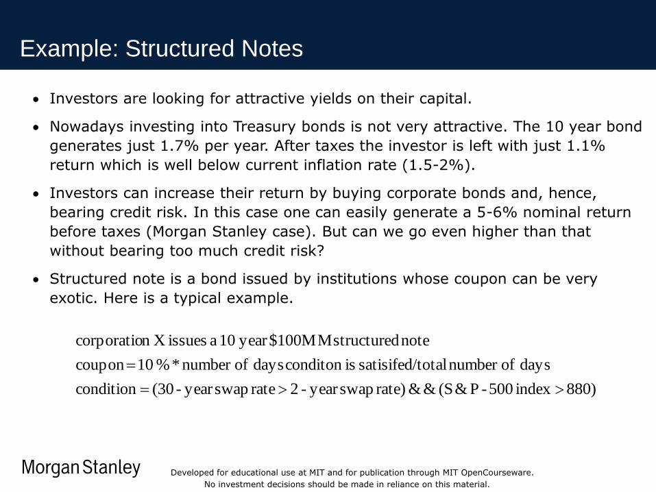
Example: Structured Notes

Investors are looking for attractive yields on their capital.

Nowadays investing into Treasury bonds is not very attractive. The 10 year bond

generates just 1.7% per year. After taxes the investor is left with just 1.1%

return which is well below current inflation rate (1.5-2%).

Investors can increase their return by buying corporate bonds and, hence,

bearing credit risk. In this case one can easily generate a 5-6% nominal return

before taxes (Morgan Stanley case). But can we go even higher than that

without bearing too much credit risk?

Structured note is a bond issued by institutions whose coupon can be very

exotic. Here is a typical example.

880) index 500-P&(S && rate) swapyear - 2 rate swapyear -(30 condition

days ofnumber totalsatisifed/ isconditon days ofnumber * % 10 coupon

note structured $100MMyear 10 a issues Xn corporatio



Only Source /


line

Guide @ 2.68

Guide @ 1.64

Guide @ 1.95


Guide @ 2.80


Guide @ 0.22

Guid

e @

4.6

9

Structured Notes: Coupon Enhancement

The bond holder bears tail risk: The historical probability of events is low but the

market implied probability of them is significant, so that the investor can obtain

a coupon enhancement.

What will the institution who sold the bond do? First, the note is priced using a

Monte Carlo simulation which was described in the presentation. Next, deltas

with respect to equity, rates, and credit will be calculated and the note will be

hedged accordingly.

For the described structured note the breakdown of the condition implies a very

severe recession.



Only Source /


line

Guide @ 2.68

Guide @ 1.64

Guide @ 1.95


Guide @ 2.80


Guide @ 0.22

Guid

e @

4.6

9

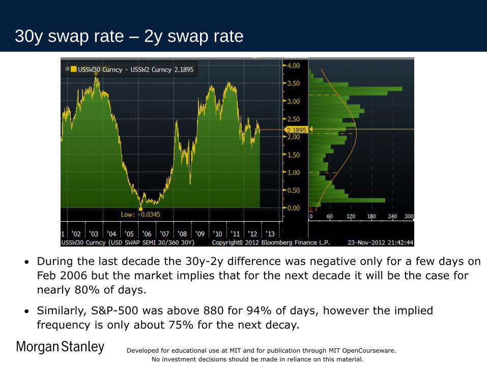
30y swap rate – 2y swap rate

During the last decade the 30y-2y difference was negative only for a few days on

Feb 2006 but the market implies that for the next decade it will be the case for

nearly 80% of days.

Similarly, S&P-500 was above 880 for 94% of days, however the implied

frequency is only about 75% for the next decay.



Only Source /


line

Guide @ 2.68

Guide @ 1.64

Guide @ 1.95


Guide @ 2.80


Guide @ 0.22

Guid

e @

4.6

9

34 34 34

Disclosures

The information herein has been prepared solely for informational purposes and is not an offer to buy or sell or a solicitation of an offer to buy or sell any security or instrument or to participate

in any trading strategy. Any such offer would be made only after a prospective participant had completed its own independent investigation of the securities, instruments or transactions and

received all information it required to make its own investment decision, including, where applicable, a review of any offering circular or memorandum describing such security or instrument,

which would contain material information not contained herein and to which prospective participants are referred. No representation or warranty can be given with respect to the accuracy or

completeness of the information herein, or that any future offer of securities, instruments or transactions will conform to the terms hereof. Morgan Stanley and its affiliates disclaim any and all

liability relating to this information. Morgan Stanley, its affiliates and others associated with it may have positions in, and may effect transactions in, securities and instruments of issuers

mentioned herein and may also perform or seek to perform investment banking services for the issuers of such securities and instruments.

The information herein may contain general, summary discussions of certain tax, regulatory, accounting and/or legal issues relevant to the proposed transaction. Any such discussion is

necessarily generic and may not be applicable to, or complete for, any particular recipient's specific facts and circumstances. Morgan Stanley is not offering and does not purport to offer tax,

regulatory, accounting or legal advice and this information should not be relied upon as such. Prior to entering into any proposed transaction, recipients should determine, in consultation with

their own legal, tax, regulatory and accounting advisors, the economic risks and merits, as well as the legal, tax, regulatory and accounting characteristics and consequences, of the transaction.

Notwithstanding any other express or implied agreement, arrangement, or understanding to the contrary, Morgan Stanley and each recipient hereof are deemed to agree that both Morgan

Stanley and such recipient (and their respective employees, representatives, and other agents) may disclose to any and all persons, without limitation of any kind, the U.S. federal income tax

treatment of the securities, instruments or transactions described herein and any fact relating to the structure of the securities, instruments or transactions that may be relevant to understanding

such tax treatment, and all materials of any kind (including opinions or other tax analyses) that are provided to such person relating to such tax treatment and tax structure, except to the extent

confidentiality is reasonably necessary to comply with securities laws (including, where applicable, confidentiality regarding the identity of an issuer of securities or its affiliates, agents and

advisors).

The projections or other estimates in these materials (if any), including estimates of returns or performance, are forward-looking statements based upon certain assumptions and are preliminary

in nature. Any assumptions used in any such projection or estimate that were provided by a recipient are noted herein. Actual results are difficult to predict and may depend upon events outside

the issuer’s or Morgan Stanley’s control. Actual events may differ from those assumed and changes to any assumptions may have a material impact on any projections or estimates. Other events

not taken into account may occur and may significantly affect the analysis. Certain assumptions may have been made for modeling purposes only to simplify the presentation and/or calculation of

any projections or estimates, and Morgan Stanley does not represent that any such assumptions will reflect actual future events. Accordingly, there can be no assurance that estimated returns or

projections will be realized or that actual returns or performance results will not be materially different than those estimated herein. Any such estimated returns and projections should be viewed

as hypothetical. Recipients should conduct their own analysis, using such assumptions as they deem appropriate, and should fully consider other available information in making a decision

regarding these securities, instruments or transactions. Past performance is not necessarily indicative of future results. Price and availability are subject to change without notice.

The offer or sale of securities, instruments or transactions may be restricted by law. Additionally, transfers of any such securities, instruments or transactions may be limited by law or the terms

thereof. Unless specifically noted herein, neither Morgan Stanley nor any issuer of securities or instruments has taken or will take any action in any jurisdiction that would permit a public

offering of securities or instruments, or possession or distribution of any offering material in relation thereto, in any country or jurisdiction where action for such purpose is required. Recipients

are required to inform themselves of and comply with any legal or contractual restrictions on their purchase, holding, sale, exercise of rights or performance of obligations under any transaction.

Morgan Stanley does not undertake or have any responsibility to notify you of any changes to the attached information.

With respect to any recipient in the U.K., the information herein has been issued by Morgan Stanley & Co. International Limited, regulated by the U.K. Financial Services Authority. THIS

COMMUNICATION IS DIRECTED IN THE UK TO THOSE PERSONS WHO ARE MARKET COUNTERPARTIES OR INTERMEDIATE CUSTOMERS (AS DEFINED IN THE UK

FINANCIAL SERVICES AUTHORITY’S RULES).

ADDITIONAL INFORMATION IS AVAILABLE UPON REQUEST.



MIT OpenCourseWarehttp://ocw.mit.edu

18.S096 Topics in Mathematics with Applications in FinanceFall 2013

For information about citing these materials or our Terms of Use, visit: http://ocw.mit.edu/terms.

http://ocw.mit.edu

http://ocw.mit.edu/terms

HJM Model for Interest Rates and Credit - MIT … 24 HJM Model for Interest Rates and Credit Denis...

Documents

Transcript of HJM Model for Interest Rates and Credit - MIT … 24 HJM Model for Interest Rates and Credit Denis...