HITS: Hurricane Intensity and Track Simulator with North...

HITS: Hurricane Intensity and Track Simulator with North AtlanticOcean Applications for Risk Assessment

J. NAKAMURA

Lamont-Doherty Earth Observatory, Columbia University, Palisades, New York

U. LALL

Columbia University, New York, New York

Y. KUSHNIR

Lamont-Doherty Earth Observatory, Columbia University, Palisades, New York

B. RAJAGOPALAN

University of Colorado Boulder, Boulder, Colorado

(Manuscript received 9 June 2014, in final form 16 March 2015)

ABSTRACT

Anonparametric stochasticmodel is developed and tested for the simulation of tropical cyclone tracks. Tropical

cyclone tracks demonstrate continuity and memory over many time and space steps. Clusters of tracks can be

coherent, and the separation between clusters may be marked by geographical locations where groups of tracks

diverge as a result of the physics of the underlying process. Consequently, their evolutionmay be non-Markovian.

Markovian simulation models, as are often used, may produce tracks that potentially diverge or lose memory

quicker than happens in nature. This is addressed here through a model that simulates tracks by randomly

sampling track segments of varying length, selected from historical tracks. For performance evaluation, a spatial

grid is imposed on the domain of interest. For each grid box, long-term tropical cyclone risk is assessed through the

annual probability distributions of the number of storm hours, landfalls, winds, and other statistics. Total storm

length is determined at birth by local distribution, andmovement to other tropical cyclone segments by distance to

neighbor tracks, comparative vector, and age of track. The model is also applied to the conditional simulation of

hurricane tracks from specific positions for hurricanes that were not included in the model fitting so as to see

whether the probabilistic coverage intervals properly cover the subsequent track. Consequently, tests of both the

long-term probability distributions of hurricane landfall and of event simulations from the model are provided.

1. Introduction

Extreme weather events such as tropical cyclones

occur with low frequency. Because of the low proba-

bility of North Atlantic Ocean tropical cyclone landfall,

landfall statistics are difficult to estimate. Statistical

methods can be employed to resample the historical

data, creating a large number of tracks used to improve

estimates of the probability extremes. These statistics

are useful for insurance companies in determining pre-

miums, and for communities and governments in de-

termining disaster plans and building codes.

Several models have been introduced to estimate tropi-

cal cyclone landfall probabilities. Some directly simulate

tropical cyclone landfall and intensity by Monte Carlo

methods (Clark 1986; Chu andWang 1998), dimensionality

reduction (Buchman et al. 2011), or by fitting a probability

function (Emanuel and Jagger 2010), while others create

sets of simulated tracks (Casson and Coles 2000; Emanuel

et al. 2006; Hall and Jewson 2007; T.M.Hall and S. Jewson

2008, unpublished manuscript, available at http://arxiv.org/

pdf/0801.1013v1.pdf; Hallegate 2007; Rumpf et al. 2007,

2009; Vickery et al. 2000; Yonekura and Hall 2011).

Corresponding author address: Jennifer Nakamura, Ocean and

Climate Physics, 103F Oceanography, Lamont-Doherty Earth Ob-

servatory, P.O. Box 1000/61 Rte. 9W, Palisades, NY 10964-8000.

E-mail: [email protected]

1620 JOURNAL OF APPL IED METEOROLOGY AND CL IMATOLOGY VOLUME 54

DOI: 10.1175/JAMC-D-14-0141.1

� 2015 American Meteorological Society

http://arxiv.org/pdf/0801.1013v1.pdf


mailto:[email protected]

Vickery et al. (2000) used a 58 3 58 box to determine

track heading, speed, and intensity, through a regression

of historical storm data on location attributes, prior time

step storm speed, and direction. Hurricane intensity is

modeled as a function of prior intensity for up to three

time steps and of sea surface temperature at appropriate

locations. A random innovation consistent with the re-

gressionmodel is added to generate the tracks. A number

of other parameters are also estimatedwithin a regression

framework, and landfall probability distributions are es-

timated from the simulations. The variance explained by

their regression models is typically not high, but the

conditional probability distributions derived generally

look plausible. Casson and Coles (2000) simulate tracks

by the shift of a uniform random value less than 100n mi

(1 nmi 5 1.852km) and use a simulated pressure plus

land effects to produce a simulated wind speed. Emanuel

et al. (2006) present a smoothedMarkov chainmodel and

beta and advection model using synthetic flow at 850 and

250hPa. Hallegate (2007) used the later to investigate

landfall and damage probabilities. In our work in the late

1990s, a Markov chain model was initially implemented

to simulate these popular paths with transition proba-

bilities changing from grid box to grid box, but it was

found to be too diffusive. For each grid box, the one-step

transition probability to adjoining grid boxes and to the

grid box (58) itself was estimated. The Markov chain

model was fit to the post–airplane reconnaissance his-

torical record (1944–99) and then track simulations were

generated, seeded by a random selection of historical

track birth positions. A comparison of the historical

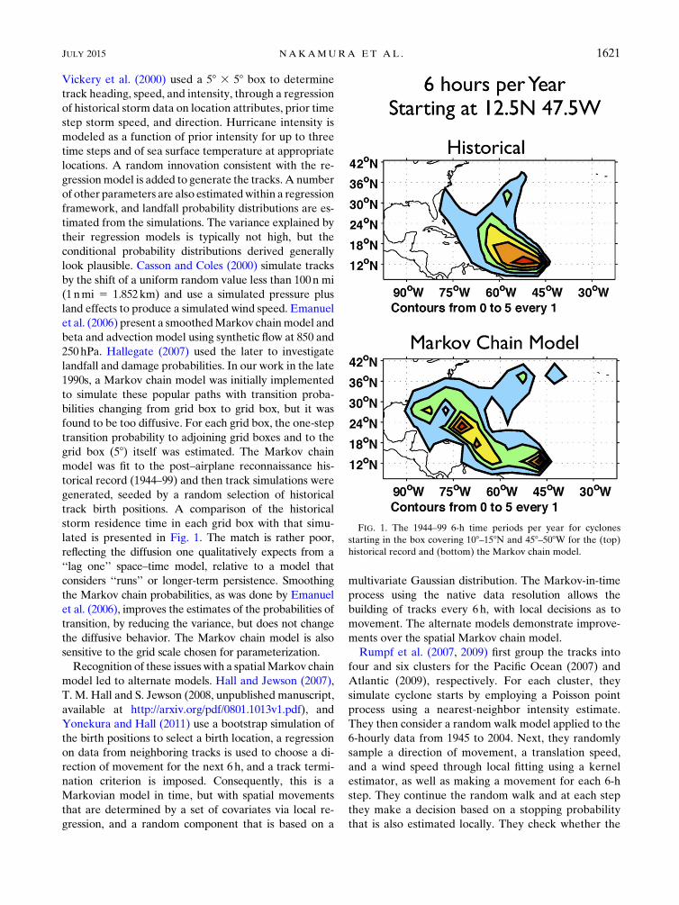
storm residence time in each grid box with that simu-

lated is presented in Fig. 1. The match is rather poor,

reflecting the diffusion one qualitatively expects from a

‘‘lag one’’ space–time model, relative to a model that

considers ‘‘runs’’ or longer-term persistence. Smoothing

the Markov chain probabilities, as was done by Emanuel

et al. (2006), improves the estimates of the probabilities of

transition, by reducing the variance, but does not change

the diffusive behavior. The Markov chain model is also

sensitive to the grid scale chosen for parameterization.

Recognition of these issues with a spatialMarkov chain

model led to alternate models. Hall and Jewson (2007),

T. M. Hall and S. Jewson (2008, unpublished manuscript,

available at http://arxiv.org/pdf/0801.1013v1.pdf), and

Yonekura and Hall (2011) use a bootstrap simulation of

the birth positions to select a birth location, a regression

on data from neighboring tracks is used to choose a di-

rection of movement for the next 6h, and a track termi-

nation criterion is imposed. Consequently, this is a

Markovian model in time, but with spatial movements

that are determined by a set of covariates via local re-

gression, and a random component that is based on a

multivariate Gaussian distribution. The Markov-in-time

process using the native data resolution allows the

building of tracks every 6h, with local decisions as to

movement. The alternate models demonstrate improve-

ments over the spatial Markov chain model.

Rumpf et al. (2007, 2009) first group the tracks into

four and six clusters for the Pacific Ocean (2007) and

Atlantic (2009), respectively. For each cluster, they

simulate cyclone starts by employing a Poisson point

process using a nearest-neighbor intensity estimate.

They then consider a random walk model applied to the

6-hourly data from 1945 to 2004. Next, they randomly

sample a direction of movement, a translation speed,

and a wind speed through local fitting using a kernel

estimator, as well as making a movement for each 6-h

step. They continue the random walk and at each step

they make a decision based on a stopping probability

that is also estimated locally. They check whether the

FIG. 1. The 1944–99 6-h time periods per year for cyclones

starting in the box covering 108–158N and 458–508W for the (top)

historical record and (bottom) the Markov chain model.

JULY 2015 NAKAMURA ET AL . 1621


generated storm conforms to the cluster that it was

generated from and use this to accept or reject the storm

that was generated. Conceptually, their approach is then

similar to that of Hall and Jewson but with a different

implementation where kernel density estimators and

classification do much of the work. In summary, the sim-

ulation models presented in the literature are by and large

Markovian, looking at ways tomarch the track one step (in

time and/or gridded space) at a time based on conditional

probabilities inferred from track and climate attributes.

The more successful models appear to consider transition

probabilities or conditional probability distributions that

changewith spatial location andwith respect to exogenous

attributes, but not with respect to the age of the track, or

the extended past history of the track.

To a first-order approximation, tropical cyclones

move in the direction that the winds (over the depth of

the storm) steer them. In the northern Atlantic, the

northeasterly trade winds move the storms westward

from the African coast. The prevailing flow around the

subtropical high curves them, and other cyclones gen-

erated in the Caribbean Sea and Gulf of Mexico,

northward approaching the North American coast and

then eastward in the middle latitudes. Elsner and Kara

(1999) call this a parabolic sweep. The position and

strength of the subtropical high, the extratropical cir-

culation, and the birth location of the tropical cyclone

varies, allowing variations in the tracks. To reflect the

parabolic sweep, and variations of it, a spatial model is

needed. More ‘‘popular’’ track paths have a higher

probability of occurring than do ‘‘unpopular’’ ones.

Considering higher dependence (e.g., to the two prior

steps) in a Markov model leads to an explosion in the

number of parameters to be estimated for the resulting

transition probability matrix, which is commonly called

the ‘‘curse of dimensionality’’ and is hence not indicated

with the hurricane track dataset. In the time series

modeling literature, the situation is often addressed by

considering a semi-Markov or Markov renewal model

(Bhat and Miller 1972; Çinlar 1969, 1975; Gilbert et al.

1972; Foufoula-Georgiou and Lettenmaier 1987). A di-

rect application of the Markov renewal model to the

tropical cyclone track setting is not obvious at first

glance, since one needs a specification of discrete states

for the system, prior to modeling the conditional distri-

bution of the time to be spent in each future state. In-

spired by the Markov renewal idea, we propose a

modeling strategy where we consider the time ti to be

spent along a candidate track i to be a random variable

and we allow the selection of the candidate track and the

associated ti to depend on location and other attributes.

This provides the basis for the hurricane intensity and

track simulator (HITS) model presented in this paper.

The historical hurricane record is discussed in section 2,

along with 2012 data used for model verification on

novel tracks. Section 3 describes the HITS algorithm

and section 4 presents the results of the comparison to

the historical record using percentiles, and a visual

comparison of distributions with split violin plots. The

last section discusses results, a brief comparison to other

hurricane track models, and plans for future work.

2. Data

The data used for the model are taken from the his-

torical best-track North Atlantic hurricane dataset

(HURDAT; Jarvinen et al. 1984) from 1851 to 2011 with

information on storm position (latitude and longitude)

and wind speed every 6h. The data were obtained from

the National Hurricane Center, and the record contains

‘‘named’’ storms, defined as storms whose maximum

sustained (1-min-averaging period) surface winds ex-

ceeded 18ms21 (34kt, or 39mih21). The primary table of

tropical cyclone data consists of the number of storms in a

year, the catalog storm number, the year, month, day, and

position on the track (6-h time step), the latitude, longi-

tude, andwind speed (kt). A domain of 58–458Nand 1008–258Wwas chosen and segmented by a 58 3 58 grid to give

120 boxes. These grids are used to report model perfor-

mance evaluation, but are not used in model fitting. The

model is built directly using the track data without spatial

discretization. During the 161-yr record, 1465 tropical

cyclones spent all or part of their lifetimes in the domain.

As a result of routine aircraft reconnaissance missions

into tropical cyclones beginning in 1944, details on the

position of the tropical cyclone eye are available. This has

led to greater accuracy in the 6-h position data in storms far

from land or shipping lanes. The storm durations in the

prior period (1851–1943) are shorter than in the sub-

sequent period (1944–2011) as a result of this change in

observing method. The birth location of the storms is

sampled from the post-1944 data. However, all available

track data are used for neighbors tomodel tropical cyclone

movement behavior, following a philosophy of nonideal

data inclusion (Halevy et al. 2009). HITS based on the

historical data was used to simulate tracks of recent storms

(not included in the model-fitting set) to test how well the

conditional simulations from a particular position of a

hurricane provide coverage of the actual hurricane track

from that point on. This is a stronger test of the algorithm

than reported by any of the previous models.

3. HITS conceptual model

Çinlar (1969) provides a formal introduction to the

Markov renewal model. Consider a finite number of


states, for example, wet or dry for rainfall. In a Markov

chain model, state transitions occur at a fixed time step

(e.g., daily), and the parameter of interest is the state

transition probability matrix for that time step. In a

Markov renewal process, the time spent (e.g., wet or dry

spell length) in each state can depend on the time spent

in the prior state. Hence, the key parameter is the con-

ditional probability distribution of the time to spend in

the new state, given the time spent in the previous state

(e.g., the wet spell duration depends on the previous dry

spell duration), or f(tk j tl), where l is the current state, kis the new state, and tl and tk are the corresponding

durations. A generalization of the Markov renewal

model to a nonhomogeneous Markov renewal model

can be obtained if the conditional probability distribu-

tions of the durations in each state are further allowed to

depend on covariates at the time of state transition. For

instance, the covariates could be the calendar month, or

an atmospheric circulation index (for the rainfall ex-

ample) such as the Pacific–North America index. In this

case the conditional probability distribution for the

model is f [tk j tl, u(t)], where u(t) represents a vector of

covariates at the time t, when the transition (l, k) takes

place.

Hurricane tracks are often well organized in a region.

For instance, Nakamura et al. (2009) used the k-means

algorithm with the geometry of hurricane tracks to

identify six clusters associated with Atlantic hurricanes.

One could consider each of these clusters as a state, and

consider the development of a renewal model for the

transition of a hurricane across these clusters. However,

this not led to a conceptually or practically attractive

model for simulating hurricane tracks. At the same time,

we recognize that while a hard clustering model, such as

k-means, would assign each hurricane track to a specific

cluster, a hierarchical clustering model may reveal a dif-

ferent, nested organizational structure for the tracks with

clusters and subclusters, and a probabilistic clustering

model would only assign a probability for each track to

belong to a specific cluster. Further, if we consider state

transitions across clusters, we are essentially considering

tracks that originated in one cluster tomigrate to another

cluster, and so forth. Indeed, in the Atlantic we see this

phenomenon. Tracks that originate in the eastern equa-

torial Atlantic can curve northward, continue to landfall,

or curve southward, as they approach the continental

landmass. From a hierarchical clustering perspective,

these would represent the subclusters of perhaps a lower-

level cluster, and the possibility of transition across these

subclusters exists, especially at certain geographical re-

gions, and/or at certain times into the trajectory.

Given these observations, we consider the following

approach. Instead of explicitly identifying clusters of

hurricane tracks at the outset, we consider the possibility

that the observed hurricane tracks are stochastic re-

alizations of possible tracks that could occur under a

particular state of a hurricane-generating process. These

states are latent or unobserved by us, but intuitively they

correspond to the clusters or subclusters we try to identify

from observed hurricane data. An observed hurricane

track would then be a realization of a sequence of tran-

sitions between these latent states. In other words, a

hurricane track could be born in a state associated with

genesis in the eastern equatorial Atlantic, evolve as per

this state’s dynamics for a certain number of time steps,

and then undergo a state transition to a latent state that

conforms to curving north, curving south, or proceeding to

landfall. This process could then repeat until a complete

track is realized. A similar concept underlies the hidden

Markovmodel (Hughes et al. 1999; Robertson et al. 2004)

that is often used for downscaling precipitation from

climate models. Latent states that govern regional

precipitation dynamics and their transitions on a daily

time step are identified based on the precipitation time

series from multiple stations. The state transition

probability could depend on the geographical location,

as well as other attributes such as the wind shear, the

surface temperature field, the state of ENSO or NAO,

or other covariates. This corresponds to the non-

homogeneous hidden Markov model (Mehrotra and

Sharma 2005; Kwon et al. 2009) for precipitation and,

in our case, a nonhomogeneous hidden Markov re-

newal model (NHMRM).

The practical implementation of this idea into a space–

time simulator for hurricane tracks is described next. A

nonparametric approach based on k-nearest neighbor

density estimation is used to develop the conditional

simulation strategy implied by the NHMRM. Note that

we do not try to formally estimate a parametric model for

the NHMRM, but devise a resampling strategy that al-

lows the construction of new simulated tracks assuming

that each track segment is a realization from a latent state

of the hurricane-generating process, and that the identi-

fication of the next track segment to resample corre-

sponds to sampling from an underlying state transition.

To introduce some notation, laid out in the appendix,

let us consider a latent state i, a current position x*, and a

historical hurricane track C(x*) that passes through x*.

Now consider CB(x*) as the set of all historical hurricane

tracks that pass through a region B(x*) of a certain ra-

dius centered around x*. Each of the tracks in CB(x*)

corresponds to a different latent state associated with

the hurricane process, and based on its proximity is

considered a candidate realization of a transition to that

latent state. Hence, if during the simulation, we

consider a shift from a trackC(x*) to one of the tracks in


the set CB(x*) that would correspond to a transition

from a latent state l to any of the other latent states,

including l, since other tracks can also conform to the

same underlying state. We consider that the probability

of such a transition depends on specific geometrical and

other attributes of each track in the set CB(x*).

Since, we are interested in simulating hurricane tracks

under NHMRM, but not necessarily in identifying the

latent states as part of the process, we can consider a

simulated track C(x) as a random curve, whose pieces

are determined by successive transitions across histori-

cal tracks at a sequence of randomly selected candidate

locations, an example of which is x*. Once a transition

occurs, as per the renewal model, the time to spend,

t[C(x*)], in a realization from that latent state, that is,

along the newly chosen track, C(x*), needs to be sim-

ulated. This defines a new position x* that is t steps

beyond the previous location, and the process is then

repeated. The evolution of C(x) in space and time may

then be represented through a conditional probability

distribution:

ffC(x*), t[C(x*)] j u(x*)g ,

where u(x*) represents a set of covariates at the location

x* that includes attributes of the current state as repre-

sented by the hurricane track arriving at x*. Thus,

given a certain location, the model considers the selec-

tion of a state going forward from that location, and the

time that is to be spent following that track. This permits

one to consider persistence of motion along tracks and

avoids the diffusion associated with the one-step Mar-

kov chain models.

The u(x*) is a set of parameters relevant to the tropical

cyclone process that vary by location. The u(x*) may in-

clude, for instance, the geographical location of x*, the

index and direction vector of the trackC(x*)5 i that was

traveled to reach the location x*, atmospheric variables

that influence track selection, and large-scale climate

variables, such as sea surface temperatures or indices

such as the Niño-3.4 or NAO. The specific choices for

u(x*) made in the application presented here, and the

nonparametric estimation of the conditional probability

density function ffC(x*), t[C(x*)] ju(x*)g, which is used

to simulate the tracks, are discussed below as part of the

algorithm presentation.

The HITS algorithm for simulating tropical cyclone

tracks steps through time in 6-h intervals, making de-

cisions along the path as to which historical track to

follow. This process repeats itself until the lifetime is

met. The total duration of a hurricane is also a model

parameter that is randomly sampled in an initial step. A

schematic of the process is provided in Fig. 2.

HITS algorithm

The implementation of the nonparametric resampling-

based algorithm for the application of the NHMRM to

theAtlantic sector is presented below. The state variables

of the model define the latent states: the time spent in

each state. The latent states are manifest in a realization

as segments of historical hurricane tracks. In addition,

the genesis location of each track simulated, the total life

of each track, and the number of tracks to simulate for

each season are all random variables.

The associated data and the simulation code are

available from the authors. We consider the simulation

of a hurricane season at a time, and can generate as

many hurricane seasons as desired. For each simulated

hurricane season, the following steps are taken:

1) Select the number of storms for the season:

N;U(Nl,Nu) , (1)

where N is the number of storms in a simulated

season, Nl is the lowest number, and Nu is the

highest number of storms during the years 1944–

2011, whileU( ) is a uniform draw, a bootstrap of the

historical counts per year (Efron 1979). This can be

conditioned on the observed or modeled large-scale

climate state to reflect the dependence of number of

tropical cyclone births on ENSO or other climate

FIG. 2. Abbreviated flowchart of the HITS algorithm presenting an

illustration of the steps in the process.


states. However, in the work presented here, we do

not consider such a dependence.

2) For each potential storm, randomly select a birth

location (first track position) pb from all historical

births post-1944 or historical births for years corre-

sponding to a specific condition (El Niño, positionof the Bermuda high, etc.):

pb ;U[G(pb)] , (2)

where G(pb) is a set of all candidate birth loca-

tions (first locations of each post-1944 track in the

HURDAT dataset). In the applications presented

in this paper we choose the birth location uncondi-

tionally from the candidate locations.

3) Sample the simulated track lifetime:

L;U(L1,L2) , (3)

where L is the entire duration of the cyclone in

6-h time steps, and L1 and L2 are the minimum

and maximum total lifetimes of the tracks that lie

in B(pb), where B(pb) is an area with a 2.58 radiusaround pb, Tracks recorded in the years 1944–2011

are considered.

4) Define new position on the chosen track i (selected

in step 2):

pj5 p(tj) , (4)

where pj is the position on the simulated track at

iteration j and tj is the number of 6-h time steps

represented by t[C(x*)], the random amount of

time in this state, to take along chosen track i

moving forward from pb. t[C(x*)];U(t*,L), where

t* is the time elapsed on the current track and L is

the simulated track length in 6-h steps.

5) The multivariate distance criteria u(x*) of the

distance from the track to the current position,

the vector difference in direction of movement

relative to the current track, and the age (step

number) relative to the current track were used to

statistically capture and display the dynamical

behavior differences of tropical cyclones born in dif-

ferent parts of the basin through the conditional pro-

bability density function, ffC(x*), t[C(x*)] ju(x*)g.These variables are in essence surrogates for the

physics of storm movement ensuring that jumps are

made to similar neighbor tracks. Six clusters of

North Atlantic tropical cyclone tracks were iden-

tified that display differing genesis locations,

track shapes, intensities, life spans, landfalls,

seasonal patterns, and trends (Nakamura et al.

2009). The relation of genesis location to life span

(age) and preferred grouped paths (distance from

the current position and the vector difference in

the direction of movement) was considered on

this basis.

Choose a track during the years 1851–2011 by

drawing from ‘‘neighbor’’ tracks using the condi-

tional density function defined through a product

kernel density function as

ffC(x*), t[C(x*)] j u(x*)g} k(u1ij)k(u2ij)k(u3ij) ,

(5a)

where

K(u)5 (12 u2)2 (5b)

is the bisquare kernel function and u1, u2, and u3represent distance measures in terms of different

conditioning variables, as described below.

(i) The distance of a candidate historical track to

the current track is

u1 }D

2. 5(p/180); D# 2. 58 , (5c)

where D is the distance in degrees between

neighbor track points in spherical geometry.

(ii) The orientation of a candidate historical track

relative to the current track is

u2 }V

Max(V); V5 (Vxn2Vxi)

21 (Vyn2Vyi)2,

(5d)

where Max(V) is the maximum wind vector

difference over all tracks in knots, Vx is the

instantaneous storm maximum wind speed in

knots times the cosine of the angle between

the current point and the next point on the

track, Vy is the wind speed in knots times the

sine of the angle, subscript i is the current

track, and subscript n is the neighbor track.

(iii) The age of the candidate historical track

relative to the current track is

u3 }T

Max(T); T5Tn 2Ti , (5e)

where T is age of the neighbor track, in 6-h

steps, minus the age of the current track;

Max(T) is the maximum T in 6-h steps over

all tracks; subscript i refers to the current

track; and subscript n refers to the neighbor

track.

6) The 6-h steps remaining to the simulated storm end

(Rj) are calculated as


Rj 5L2 aj , (6)

where L is the duration selected in step 3 and aj is

the age at iteration j.

7) The 6-h steps to take along chosen track i (Sj) are

found by

Sj ;U(1,Rj) , (7)

where Rj is selected in step 6.

8) The positions in 6-h steps on simulated track at

iteration j are

pj 5 pb 1Sj . (8)

9) If Sj 5 Rj then stop, else repeat steps 5–8.

10) Repeat steps 2–9, N (selected in step 1) times to

complete a simulated season.

A numerical procedure for the efficient sampling and

simulation of tracks was developed. A functional table was

created that recorded the storm number, position on the

track, latitude, longitude, number of time steps to the end

of the track, the comparative vector of the storm direction,

and wind speed. A second lookup table was created that

listed the ‘‘neighbors’’ for all tracks for each position in

each track.Neighbors are all points on other trackswithin a

2.58 radius of the current location with a given probability

basedon thebisquare kernel function [(5b)] tomove to that

location based on distance, comparative vector, and age in

6-h steps as defined in step 5 in (5a)–(5e).

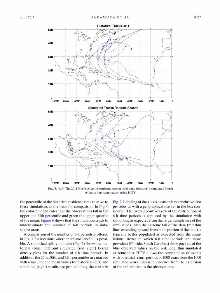
As an example, Fig. 3 shows the actual 2011 North At-

lantic hurricane season tracks (top), and aHITS algorithm

simulation of an arbitrary hurricane season plotted at the

bottom. Figure 3 (bottom panel) shows that the tracks

havemore variation than the historical tracks, but they are

still more coherent than the tracks from theMarkov chain

model in Fig. 1. Figure 3 (bottom panel) also illustrates the

jumps of the simulated tracks as they move to neighbors;

however, the accuracy of the model is assessed on the

binned statistics in section 4 rather than the track paths.

Movement to other tracks is realistic in terms of cyclone

movement as track segments are selected by criteria of

distance [(5c)], direction and speed vector [(5d)], and

similar age [(5e)]. Consider a competing Markov chain

model set up on a 18 3 18 or 2.58 3 2.58 discretization.Clearly, in that sort of a model one would have a jump of

that magnitude in every time step and have highly dis-

continuous trajectories relative to observed trajectories or

to those simulated by HITS.

4. Results

We present results for two types of tests. First, we

present results for the statistics associated with the

simulation of 1000 hurricane seasons. Next, we explore

the conditional simulation of ensembles of tracks from

different starting positions for real hurricanes (Sandy

and Isaac) from 2012 that were not included in the

model-fitting process.

The performance of the simulations for the 1000 seasons

is judged through a variety of performance measures:

(i) comparing the average spatial distribution of the

historical and simulated data,

(ii) comparing percentiles of the residence time in each

grid box,

(iii) landfall statistics, and

(iv) comparing the frequency of 6-h periods of hurricane

strength wind (.64kt).

a. Comparing the average spatial distribution of thehistorical and simulated data

The track points for the post-1944 data at 6-h time steps

are binned into boxes, and the count in each box is

recorded. This number was divided by the total number of

years of data (68) to compute mean annual values. The

observations are heavily clustered along the curve of

the parabolic sweep with a maximum off the coast of the

southern United States (Fig. 4, top panel). Storm starting

locations, being of particular interest, were also binned and

plotted (Fig. 4, bottom panel). Births are clustered pri-

marily in four regions covering approximately eight boxes,

each having as many as 25 births over the 68 seasons.

Figure 5 shows the simulated corresponding figure of

the mean 6-h periods (top panel) and births (bottom

panel). The 6-h periods are slightly overestimated in the

mean below 248N and underestimated above that lati-

tude. Exiting the tropics and entering the extratropics,

cyclones are subjected to strong wind speeds and the 6-h

observations are farther apart. In an alternate run (not

shown), a 58 radius is employed rather than the 2.58threshold. This change decreases the underestimation

above 248N; however, it greatly increases the over-

estimation below that latitude. Mean simulated starts

(Fig. 5, bottom panel) slightly overestimate the tropical

cyclone births off the coast of Africa, which may be the

cause of the slight increase in the number of 6-h periods

found there. Since these are randomly sampled un-

conditionally from the historical set, the difference is

purely due to sampling variations.

b. Comparing percentiles of the residence time in eachgrid box

The spatial structure of the simulated tracks was

assessed through a comparison of the number of 6-h

time steps in each box relative to the historical data.

Since we have 1000 simulations fromHITS, we compute


the percentile of the historical residence time relative to

these simulations as the basis for comparison. In Fig. 6

the color blue indicates that the observations fall in the

upper one-fifth percentile and green the upper quartile

of the mean. Figure 6 shows that the simulation tends to

underestimate the number of 6-h periods in data-

sparse areas.

A comparison of the number of 6-h periods is offered

in Fig. 7 for locations where mainland landfall is possi-

ble. A smoothed split violin plot (Fig. 7) shows the his-

torical (blue, left) and simulated (red, right) kernel

density plots for the number of 6-h time periods. In

addition, the 25th, 50th, and 75th percentiles are marked

with a line, and the mean values for historical (left) and

simulated (right) results are printed along the x axis in

Fig. 7. Labeling of the x-axis location is not inclusive, but

provides us with a geographical marker in the box con-

sidered. The overall positive skew of the distribution of

6-h time periods is captured by the simulation with

smoothing as expected from the larger sample size of the

simulations. Also the extreme tail of the data (red thin

lines extending upward frommain portion of the data) is

typically better populated as expected from the simu-

lations. Boxes in which 6-h time periods are more

prevalent (Florida, South Carolina) show pockets of the

blue observed values on the red, long, thin simulated

extreme tails. HITS allows the computation of events

with potential return periods of 1000 years from the 1000

simulated years. This is in evidence from the extension

of the tail relative to the observations.

FIG. 3. (top) The 2011 North Atlantic hurricane season tracks and (bottom) a simulated North

Atlantic hurricane season using HITS.


The historical distribution is occasionally multi-

modal while the simulated case is unimodal, reflecting

the smoothing from the larger sample size. Differences

in the underlying probability distributions of the his-

torical and simulated results are tested using a two-

sample Kolmogorov–Smirnov (KS) and Cramer–von

Mises (CM) tests. Both the KS and CM tests are non-

parametric and compare the location and shape of the

empirical cumulative distribution functions of the two

samples. All but one of the boxes (Virginia) pass the

KS and CM tests at the 5% significance level indicating

the same underlying probability distributions. Mean

values of historical and simulated distributions along

the y axis are similar, along with their distribution

shapes. However, the median historical values fall

between the 25th and 75th percentiles of the HITS

simulations in all cases except for the low-populated

Texas box.

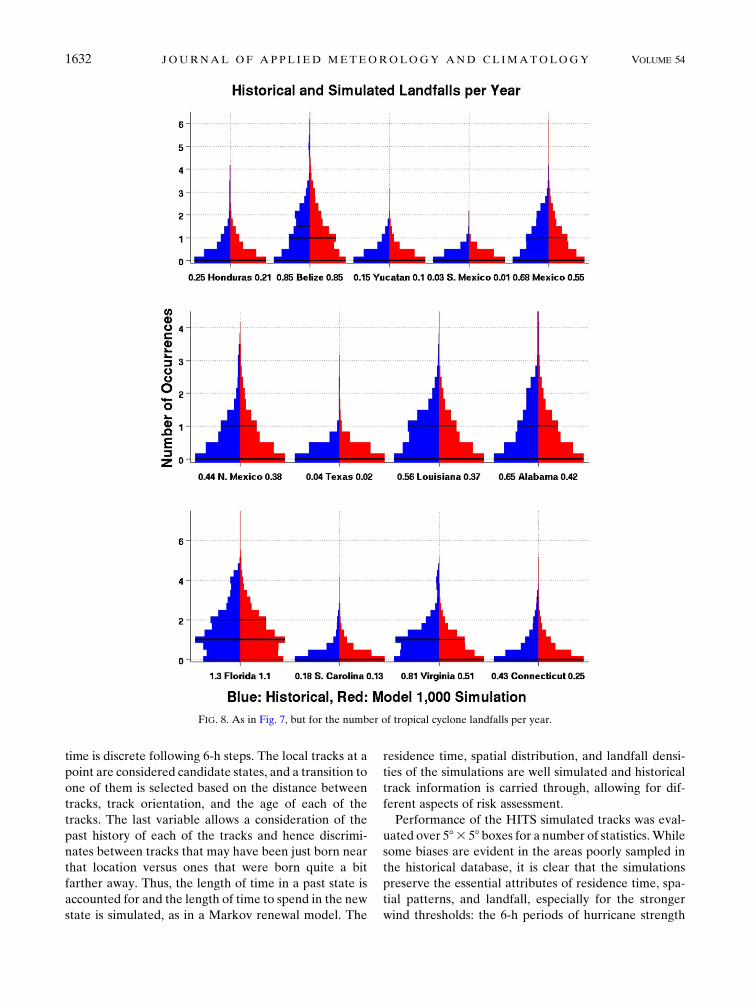
c. Landfall statistics

A land–sea mask was created to indicate which boxes

in the domain are considered mainland and which are

ocean. From that it was possible to count the storms

(both historical and simulated) as they crossed from

ocean to the mainland, and vice versa. A smoothed split

violin plot of historical (blue, left) and simulated (red,

right) distributions of mainland landfalls is shown in

Fig. 8. The width of the histogram is normalized to a

maximum width equal to 0.9; the 25th, 50th, and 75th

percentiles are marked with a line; and the mean values

for historical (left) and simulated (right) results are

printed along the x axis of Fig. 8. Distributions of land-

falls are remarkably similar between the historical and

simulated datasets. In a majority of the boxes the simu-

lated extreme tail extends beyond the historical (Belize,

Yucatan, Mexico, Louisiana, Florida, South Carolina,

FIG. 4. (top) Average number of historical (1944–2011) hurricane 6-h time periods per year

binned into 58 3 58 grid boxes and (bottom) number of historical tropical cyclone starts per box.


and Connecticut). The remaining landfall boxes are

matched by the historical extreme value, except in Texas,

where the result is underestimated. The Texas box ap-

pears in Fig. 6 as an area in which the low density of

historical tracks leads to an underestimation of simulated

tracks in those regions (median of the historical is above

the 75th percentile of the simulation). As in the 6-h-per-

year violin (Fig. 7), all but one of the boxes (Virginia)

passes the KS and CM tests at the 5% significance level,

indicating that the underlying probability distributions of

the historical and simulated datasets are the same.

d. Comparing frequency of 6-h periods of hurricanestrength wind (.64kt)

Wind speed information (as well as any other track

information in the HURDAT dataset) associated with

the historical tracks is retained in the simulated tracks.

For 6-h time periods of hurricane strength (33m s21,

64 kt, or 74mi h21) and above, a smoothed split violin

plot (Fig. 9) shows the historical (left, blue) and simulated

(right, red) distributions in mainland landfall areas. The

hurricane strength statistic is a subset of the 6-h time

periods per year (Fig. 7), but the distribution of counts is

different for the two: smoother and shorter simulation

tails. The historical and simulated means are closer in

value for the hurricane-strength cases (Fig. 9) than for the

results for the 6-h time periods per year (Fig. 7), although

the overall numbers of occurrences are reduced. All

boxes pass the KS and CM tests at the 5% significance

level indicating that the underlying probability distribu-

tions of the historical and simulated results are the same.

e. 2012 hurricanes

Since HITS was fit using the HURDAT dataset of

1851–2011, an ‘‘out of’’ sample of HITS on 2012 tracks

was made by selecting different positions on a hurricane

FIG. 5. (top) Average number of simulated hurricane 6-h time periods per year binned into

58 3 58 grid boxes and (bottom) number of historical tropical cyclone starts per box times 68 to

match the historical record of 1944–2011.


track from which to simulate. This is a different way of

applying the same model. Instead of looking at long-

term simulations, one looks at a given hurricane track

at a particular stage and, using the conditional distri-

bution of trajectory and intensity given a position on the

track, generates forward simulations. This was applied

to several historical hurricanes with similar results.

Here, we present the comparisons for two recent hur-

ricanes: Isaac and Sandy from 2012. In each case, dif-

ferent starting positions for the conditional simulation

were considered prior to landfall, and 1000 simulations

were performed for each starting position. These are

compared with the NOAA hurricane forecasts from the

same locations.

Text files of latitude, longitude, and wind speed

measurements every 6 h, as in the HURDAT dataset,

were taken from the Atlantic Hurricane Track Map and

Images Internet page of The Johns Hopkins University

(http://fermi.jhuapl.edu/hurr/index.html). The 5-day track

forecast, uncertainty cone, and watch/warning images

were obtained from National Weather Service’s Na-

tional Hurricane Center, while the near-surface daily

wind speed over land and ocean were taken from the

NCEP–NCAR reanalysis dataset’s (Kistler et al. 2001)

0.9950 sigma level.

1) SANDY

Sandy was a devastating storm in 2012, making land-

fall in Jamaica as a category 1 storm on the Saffir–

Simpson hurricane wind scale, in Cuba as a category 3,

and in southern New Jersey as a post–tropical cyclone,

with a significant storm surge in themid-Atlantic andNew

England states (Blake et al. 2013). Figures 10a–d show,

respectively, the HITS hurricane wind strength area in

6-h time periods per year, the maximum sustained winds

from 26 to 31 October 2012, the simulated mainland

landfalls, and the watch/warning images from the Na-

tional Hurricane Center (d) for at 1700 eastern daylight

time (EDT) on 26 October 2012. Black circles in

Figs. 10a–c mark the actual path of Hurricane Sandy

with the large black X in each of the panels indicating

where the simulation was started.

On 26October, 3 days before landfall in southernNew

Jersey, Sandy was off the Florida coast with HITS

showing high values of hurricane strength 6-h time pe-

riods and mainland landfalls along the eastern coast.

The actual path of Sandy in Fig. 10a is within the HITS

hurricane strength wind area over the ocean. The solid

contour in Fig. 10b indicates Sandy’s maximum sus-

tained hurricane strength winds and is similar to the size

and shape of the simulated hurricane wind area in

Fig. 10a. HITSmainland landfalls in Fig. 10c have bull’s-

eyes on Florida and the mid-Atlantic. On 27 October

(not shown), HITS no longer has the maximum landfall

occurring in Florida, as the hurricane is farther north

and east by then. The NHC forecast in Fig. 10d shows

landfall in Delaware, south of the eventual landfall

location.

2) ISAAC

Hurricane Isaac passed over the Lesser Antilles,

Haiti, and eastern Cuba as a tropical storm, and in-

tensified to a category 1 hurricane before making land-

fall in southeastern Louisiana, causing storm surge and

inland flooding across southeastern Louisiana and

southern Mississippi (Berg 2013). Figures 11a–d show,

respectively, the HITS hurricane wind strength area in

6-h time periods per year, the maximum sustained winds

from 25 to 30 Aug 2012, the simulated mainland land-

falls, and the watch/warning imagery from the National

Hurricane Center at 0500 EDT 25 August 2012. Black

circles in Figs. 11a–c mark the actual path of Hurricane

Isaac with the large black X in each of the panels in-

dicating where the simulation was started.

On 25 August, Isaac was over Cuba and the actual

path in Fig. 11a was within the HITS hurricane strength

wind area over the ocean. The solid contour in Fig. 11b

indicates Isaacs’s maximum sustained hurricane

strength winds and is similar to the size and shape of the

simulated hurricane wind area in Fig. 11a. HITS main-

land landfalls in Fig. 11c have a large value over Florida

with smaller ones along the Gulf Coast, the East Coast,

and even over Central America. On 27 August (not

shown), HITS has a greater probability of landfall on the

FIG. 6. The spatial structure of the 1000 simulated tracks shown

by the percentiles of the count of 6-h time steps in each box com-

pared to the historical record (1944–2011). The color blue implies

that the observations fall in the upper one-fifth percentile, and

green indicates the upper quartile.


http://fermi.jhuapl.edu/hurr/index.html

Gulf Coast as it moves into the Gulf of Mexico. The

NHC forecast in Fig. 11d shows landfall in western

Florida, east of the actual Louisiana landfall.

5. Summary and discussion

A new, nonparametric tropical cyclone track simula-

tor that is motivated by the observation that Markovian

models tend to be diffusive relative to historical obser-

vations was presented. The basic idea, inspired by a

nonhomogeneous hidden Markov renewal model for-

mulation, considers conditional distributions of latent

states that generate hurricane tracks, through resampling

along a track using a kernel density function with

k-nearest neighbor bandwidth, applied to selected track

attributes. Samples from this nonparametric conditional

distribution function lead to the transition to a new latent

state that is realized as a shift to historical hurricane track

at each transition location. Formodel development, space

is considered to be continuous, with no gridding, while

FIG. 7. Kernel density estimation split violin plot of observed (blue) and simulated (red) 6-h

time periods per year for landfall areas. Mean values for observed and simulated results are

located along the x axis.


time is discrete following 6-h steps. The local tracks at a

point are considered candidate states, and a transition to

one of them is selected based on the distance between

tracks, track orientation, and the age of each of the

tracks. The last variable allows a consideration of the

past history of each of the tracks and hence discrimi-

nates between tracks that may have been just born near

that location versus ones that were born quite a bit

farther away. Thus, the length of time in a past state is

accounted for and the length of time to spend in the new

state is simulated, as in a Markov renewal model. The

residence time, spatial distribution, and landfall densi-

ties of the simulations are well simulated and historical

track information is carried through, allowing for dif-

ferent aspects of risk assessment.

Performance of the HITS simulated tracks was eval-

uated over 58 3 58 boxes for a number of statistics.While

some biases are evident in the areas poorly sampled in

the historical database, it is clear that the simulations

preserve the essential attributes of residence time, spa-

tial patterns, and landfall, especially for the stronger

wind thresholds: the 6-h periods of hurricane strength

FIG. 8. As in Fig. 7, but for the number of tropical cyclone landfalls per year.


winds for all mainland landfall boxes passed the KS and

CM tests at the 5% significance level, indicating that the

historical and simulated results were from the same

distribution. Even though the model is based directly on

the historical record and is nonparametric, an extension

of the tail probability distribution and smoothing of the

probability distribution of the statistics of interest is seen

relative to the historical data. Similarly, conditional

simulations of historical tracks showed propagation

dynamics that, relative to the point from which they are

started, have performance similar to those produced by

dynamical models that are in use for near-real-time

tropical cyclone forecasts. We do not suggest HITS as a

forecast model since none of the essential physics is

modeled at all. However, it seems that the information

contained in the historical tracks does contain enough of

the location-relevant physics such that the model that

simulates tracks based on geometrical similarity criteria

is able to do a conditional simulation of the tracks from

different locations. The ability of HITS to simulate in-

dividual tracks that are based on historical tracks is a

novel feature of this model.

FIG. 9. As in Fig. 7, but for hurricane strength winds.


Several track simulationmodelers have divided up the

Gulf and U.S. coasts and compared their model landfall

results with the historical HURDAT dataset [Figs. 4 and

5 and Table 1 in Hallegatte (2007), Fig. 18 in Hall and

Jewson (2007), Fig. 3 in Vickery et al. (2000), and Table 1

in Rumpf et al. (2009)], The areas are different for all

models, so they cannot be compared directly. They all use

different statistical tools to judge the ‘‘goodness’’ of the fit.

Hall and Jewson (2007) also use the number of 6-h

tropical cyclone positions per area in their Fig. 15. Em-

ulating the ‘‘Z score’’ (normalized probability of his-

torical minus simulated mean divided by historical) in

their Fig. 15d, all of the HITS boxes were between 21

and 11 except for those where historical and simulated

counts were zero, leaving an undefined value. The mean

normalized probability was 0.063. Although it is im-

portant to compare the mean (or median) of simulated

and historical data, this analysis emphasized comparing

the shape of the entire distribution as extreme events

appear on the tail end. Research has shown that not only

do tropical cyclone distributions display a heavy tail

(Figs. 7–9), but hurricane damage is also heavily tailed

(Katz 2002).

In sensitivity testing of the HITS model, the following

approaches were examined:

d A 58 radius of neighbor points was tried rather than

the 2.58 (given as D). This larger radius sampled

among unlike populations of tracks in the tropics

and was abandoned.d Several ways of computing the direction vector were

attempted: with previous, current, or future points, as

vector differences, or as distance angle vectors. Com-

puting both angles and distances with future points

(distance or angle needed to jump to next track

segment) gave the best results.d The median of track lifetimes was used rather than

random draw (given as L). Simulated track length was

unrealistic using the median, as shorter and longer

tracks were not represented.

FIG. 10. For Hurricane Sandy, (a) simulated hurricane wind strength area in 6-h time periods per year,

(b) maximum sustained winds from 26 Oct to 31 Oct 2012, (c) simulated mainland landfalls, and (d) watch/warning

image from the National Hurricane Center at 1700 EDT 26 Oct 2012. Black circles in (a)–(c) indicate the actual path

of Hurricane Sandy and a large black X indicates where the simulation was started.


d Use of only post-1944 data was explored. The best

results came from using all available data. If the

quality of the data is a concern, selection of those

tracks can be down weighted. Behavior of a system

with determinism like the paths of North Atlantic

hurricanes is best studied with all available informa-

tion on past behavior.

Our future work plan includes running the model

backward to determine where all landfalling storms in a

particular box started. We also plan to explicitly con-

sider conditioning on large-scale climate variables to see

if interannual variability in hurricane counts and tracks

can be properly simulated. As clustering results of North

Atlantic hurricane tracks have shown groupings that

display differing genesis locations, track shapes, in-

tensities, life spans, landfalls, seasonal patterns, and

trends (Nakamura et al. 2009), selecting the birth loca-

tion based on climate state would also impact the re-

sulting tracks and probabilities.

Acknowledgments. Our work was supported by NSF

Grant AGS-1003417. Research by YK and UL on this

project was partially funded by the National Oceanic

and Atmospheric Administration’s RISA Program,

Award NA10OAR4310212, for the ‘‘Consortium for

ClimateRisk in theUrbanNortheast (CCRUN).’’ Analysis

wasmade possible by Suzana Camargo’sMatlab-converted

HURDAT dataset.

APPENDIX

Alphabetical List of Terms in the HITS ConceptualModel

b Subscript indicating first recorded location of track

B Circular area of 2.58 around the first recorded

location of the selected track

C Track or curve

FIG. 11. ForHurricane Isaac, (a) simulated hurricane wind strength area in 6-h time periods per year, (b) maximum

sustained winds from 25 to 30 Aug 2012, (c) simulated mainland landfalls, and (d) watch/warning image from the

National Hurricane Center at 0500 EDT 25 Aug 2012. Black circles in (a)–(c) indicate the actual path of Hurricane

Isaac and a large black X indicates where the simulation was started.


D Distance between neighbor tracks in spherical

geometry

f( ) Indicates function of ( )

G Set of all recorded track locations within B

i Subscript of position on the historical track

j Subscript of position of the simulated track

k, l Indices of latent states

K( ) Kernel function

L Simulated track lifetime

n Subscript of position of neighbor track

N Number of tracks in the simulated season

p Position on the simulated track as number of

6-h steps

R Number of 6-h steps remaining until simulated

storm end

S Number of 6-h steps to take along the historical

track

t(x*) Time spent in a latent state at a transition from x*

u(x*) Vector of covariates for state transition from x*

T Relative age of the neighbor track

V Wind vector difference

x* Position at state transition location

x Location vector on a track

REFERENCES

Berg, R. J., 2013: Hurricane Isaac, 21 August–1 September 2012.

NOAA/NationalWeather Service/National Hurricane Center

Tropical Cyclone Rep. AL092012, 78 pp. [Available online at

http://www.nhc.noaa.gov/data/tcr/AL09012_Isaac.pdf.]

Bhat, U. N., and G. K. Miller, 1972:Elements of Applied Stochastic

Processes. J. Wiley, 414 pp.

Blake, E. S., T. B. Kimberlain, R. J. Berg, J. P. Cangialosi, and J. L.

Beven II, 2013: Hurricane Sandy, 22–29 October 2012.

NOAA/NationalWeather Service/National Hurricane Center

Tropical CycloneRep. AL182012, 157 pp. [Available online at

http://www.nhc.noaa.gov/data/tcr/AL182012_Sandy.pdf.]

Buchman, S. M., A. B. Lee, and C. M. Schafer, 2011: High-

dimensional density estimation via SCA: An example of mod-

elling of hurricane tracks. Stat. Methodol., 8, 18–30, doi:10.1016/j.stamet.2009.07.002.

Casson, E., and S. Coles, 2000: Simulation and extremal analysis of hur-

ricane events.Appl. Stat., 49, 227–245, doi:10.1111/1467-9876.00189.Chu, P.-S., and J. Wang, 1998: Modeling return periods of tropical cy-

clone intensities in the vicinity ofHawaii. J. Appl.Meteor., 37, 951–

960, doi:10.1175/1520-0450(1998)037,0951:MRPOTC.2.0.CO;2.

Çinlar, E., 1969: Markov renewal theory. Adv. Appl. Probab., 1,123–187, doi:10.2307/1426216.

——, 1975: Exceptional paper—Markov renewal theory: A survey.

Manage. Sci., 21, 727–752, doi:10.1287/mnsc.21.7.727.

Clark, K.M., 1986: A formal approach to catastrophe risk assessment

and management. Proc. Casualty Actuarial Soc., 73, 69–92.

Efron, B., 1979: Bootstrap methods: Another look at the jackknife.

Ann. Stat., 7, 1–26, doi:10.1214/aos/1176344552.Elsner, J. B., and A. B. Kara, 1999: Hurricanes of the North At-

lantic: Climate and Society. Oxford University Press, 512 pp.

Emanuel, K., andT. Jagger, 2010:Onestimating return periods. J.Appl.

Meteor. Climatol., 49, 837–844, doi:10.1175/2009JAMC2236.1.

——, S. Ravela, E. Vivant, and C. Risi, 2006: A statistical de-

terministic approach to hurricane risk assessment.Bull. Amer.

Meteor. Soc., 87, 299–314, doi:10.1175/BAMS-87-3-299.

Foufoula-Georgiou, E., and D. P. Lettenmaier, 1987: A Markov

renewalmodel for rainfall occurrences.Water Resour. Res., 23,

875–884, doi:10.1029/WR023i005p00875.

Gilbert, G., G. L. Peterson, and J. L. Schofer, 1972: Markov re-

newal model of linked trip travel behavior. J. Transp. Eng.

Div., 98, 691–704.

Halevy, A., P. Norvig, and F. Pereira, 2009: The unreasonable ef-

fectiveness of data. IEEE Intell. Syst., 24, 8–12, doi:10.1109/

MIS.2009.36.

Hall, T. M., and S. Jewson, 2007: Statistical modelling of North

Atlantic tropical cyclone tracks. Tellus, 59A, 486–498,

doi:10.1111/j.1600-0870.2007.00240.x.

Hallegatte, S., 2007: The use of synthetic hurricane tracks in

risk analysis and climate change damage assessment.

J. Appl. Meteor. Climatol., 46, 1956–1966, doi:10.1175/

2007JAMC1532.1.

Hughes, J. P., P. Guttorp, and S. P. Charles, 1999: A non-

homogeneous hidden Markov model for precipitation

occurrence. J. Roy. Stat. Soc., 48C, 15–30, doi:10.1111/

1467-9876.00136.

Jarvinen, B. R., C. J. Neumann, and M. A. S. Davis, 1984: A tropical

cyclone data tape for the North Atlantic basin, 1886–1983: Con-

tents, limitations, and uses. NOAATech.Memo. NHC 22, 21 pp.

Katz, R.W., 2002: Stochasticmodeling of hurricanedamage. J.Appl.

Meteor., 41, 754–762, doi:10.1175/1520-0450(2002)041,0754:

SMOHD.2.0.CO;2.

Kistler, R., and Coauthors, 2001: The NCEP–NCAR 50-Year

Reanalysis: Monthly means CD–ROM and documenta-

tion. Bull. Amer. Meteor. Soc., 82, 247–267, doi:10.1175/

1520-0477(2001)082,0247:TNNYRM.2.3.CO;2.

Kwon, H. H., U. Lall, and J. Obeysekera, 2009: Simulation of daily

rainfall scenarios with interannual and multidecadal climate

cycles for south Florida. Stochastic Environ. Res. Risk Assess.,

23, 879–896, doi:10.1007/s00477-008-0270-2.

Mehrotra, R., and A. Sharma, 2005: A nonparametric non-

homogeneous hidden Markov model for downscaling of

multisite daily rainfall occurrences. J. Geophys. Res., 110,

D16108, doi:10.1029/2004JD005677.

Nakamura, J., U. Lall, Y. Kushnir, and S. J. Camargo, 2009: Clas-

sifying North Atlantic tropical cyclone tracks by mass mo-

ments. J. Climate, 22, 5481–5494, doi:10.1175/2009JCLI2828.1.

Robertson,A.W., S.Kirshner, andP. Smyth, 2004:Downscalingof daily

rainfall occurrence over northeast Brazil using a hidden Markov

model. J. Climate, 17, 4407–4424, doi:10.1175/JCLI-3216.1.Rumpf, J., H. Weindl, P. Höppe, E. Rauch, and V. Schmidt, 2007:

Stochastic modelling of tropical cyclone tracks.Math. Methods

Oper. Res., 66, 475–490, doi:10.1007/s00186-007-0168-7.——, ——, ——, ——, and ——, 2009: Tropical cyclone hazard

assessment using model-based track simulation.Nat. Hazards,

48, 383–398, doi:10.1007/s11069-008-9268-9.

Vickery, P. J., P. F. Skerlj, and L. A. Twisdale Jr., 2000: Simulation of

hurricane risk in theU.S. using an empirical trackmodel. J. Struct.

Eng., 126, 1222–1237, doi:10.1061/(ASCE)0733-9445(2000)126:

10(1222).

Yonekura, E., and T. M. Hall, 2011: A statistical model of tropical

cyclone tracks in the western North Pacific with ENSO-

dependent cyclogenesis. J. Appl. Meteor. Climatol., 50, 1725–

1739, doi:10.1175/2011JAMC2617.1.


http://www.nhc.noaa.gov/data/tcr/AL09012_Isaac.pdf

http://www.nhc.noaa.gov/data/tcr/AL182012_Sandy.pdf

http://dx.doi.org/10.1016/j.stamet.2009.07.002

http://dx.doi.org/10.1016/j.stamet.2009.07.002

http://dx.doi.org/10.1111/1467-9876.00189

http://dx.doi.org/10.1175/1520-0450(1998)037<0951:MRPOTC>2.0.CO;2

http://dx.doi.org/10.2307/1426216

http://dx.doi.org/10.1287/mnsc.21.7.727

http://dx.doi.org/10.1214/aos/1176344552

http://dx.doi.org/10.1175/2009JAMC2236.1

http://dx.doi.org/10.1175/BAMS-87-3-299

http://dx.doi.org/10.1029/WR023i005p00875

http://dx.doi.org/10.1109/MIS.2009.36

http://dx.doi.org/10.1109/MIS.2009.36

http://dx.doi.org/10.1111/j.1600-0870.2007.00240.x



http://dx.doi.org/10.1111/1467-9876.00136

http://dx.doi.org/10.1111/1467-9876.00136

http://dx.doi.org/10.1175/1520-0450(2002)041<0754:SMOHD>2.0.CO;2

http://dx.doi.org/10.1175/1520-0450(2002)041<0754:SMOHD>2.0.CO;2

http://dx.doi.org/10.1175/1520-0477(2001)082<0247:TNNYRM>2.3.CO;2

http://dx.doi.org/10.1175/1520-0477(2001)082<0247:TNNYRM>2.3.CO;2

http://dx.doi.org/10.1007/s00477-008-0270-2

http://dx.doi.org/10.1029/2004JD005677

http://dx.doi.org/10.1175/2009JCLI2828.1

http://dx.doi.org/10.1175/JCLI-3216.1

http://dx.doi.org/10.1007/s00186-007-0168-7

http://dx.doi.org/10.1007/s11069-008-9268-9

http://dx.doi.org/10.1061/(ASCE)0733-9445(2000)126:10(1222)

http://dx.doi.org/10.1061/(ASCE)0733-9445(2000)126:10(1222)


HITS: Hurricane Intensity and Track Simulator with North...

Documents

Transcript of HITS: Hurricane Intensity and Track Simulator with North...