1

1

2

3

4

5

6

7

8

9

10

11

12

13

14

15

16

17

18

19

20

Historical change and future scenarios of sea level rise in

Macau and the adjacent waters

Wang Lin1, Huang Gang2, Zhou Wen3, Chen Wen4

1 Key Laboratory of Regional Climate-Environment for Temperature East Asia,

Institute of Atmospheric Physics, Chinese Academy of Sciences, Beijing 100029

2 State Key Laboratory of Numerical Modeling for Atmospheric Sciences and

Geophysical Fluid Dynamics, Institute of Atmospheric Physics, Chinese Academy of

Sciences, Beijing 100029, China

3 Guy Carpenter Asia-Pacific Climate Impact Centre, School of Energy and

Environment, City University of Hong Kong, Hong Kong, China

4 Center for Monsoon System Research, Institute of Atmospheric Physics, Chinese

Academy of Sciences, Beijing 100190, China

Revised 26 May 2015, Special Issue of Advances in Atmospheric Sciences

Correspondence to:

Gang Huang, Institute of Atmospheric Physics, Chinese Academy of Sciences, P.O.

Box 9804, Beijing 100029, China. E-mail: hg@mail.iap.ac.cn

2

21

22

23

24

25

26

27

28

29

30

31

32

33

34

35

36

37

38

39

40

41

Abstract

Under the background of climate change, Macau is very exposed to sea level rise

because of its low elevation, small size, and ongoing land reclamation. Therefore, we

evaluate sea level changes in Macau, both historical and, especially, possible future

scenarios, aiming to provide knowledge and a framework to help accommodate and

protect against future sea level rise. Sea level in Macau is now rising at an accelerated

rate, 1.35 mm/year over 1925–2010 and jumping to 4.2 mm/year over 1970–2010,

which outpaces the rise in global mean sea level. In addition, vertical land movement

in Macau contributes little to local sea level change. In the future, the rate of sea level

rise in Macau will be about 20% higher than the global average, as a consequence of a

greater local warming tendency and strengthened northward winds. Specifically, the

sea level is projected to rise 8–12, 22–51, and 35–118 cm by 2020, 2060, and 2100,

respectively, depending on the emission scenario and climate sensitivity. Under

RCP8.5 the increase in sea level by 2100 will reach 53–98 cm, and it will double that

under RCP2.6. Moreover, the sea level rise will accelerate under RCP6.0 and RCP8.5,

while remaining at a moderate and steady rate under RCP4.5 and RCP2.6. The key

source of uncertainty stems from the emission scenario and climate sensitivity, among

which the discrepancies in sea level rise are small during the first half of the 21st

century but begin to diverge thereafter.

Keywords: Macau, sea level rise, emission scenario, climate sensitivity, vertical land

movement, uncertainty

3

43

44

45

46

47

48

49

50

51

52

53

54

55

56

57

58

59

60

61

1 Introduction 42

Macau (22°10′N 113°33′E), a special administrative region of China, is located on

the southern coast of China, on the South China Sea (Figure 1). Its territory consists

of Macau Peninsula and the islands of Taipa and Coloane, totaling 30.3 km2 up to

2014. In fact, the total area of Macau was only 2.78 km2 in the 17th century, but it has

been enlarged by 50% since 1912 because of land reclamation efforts. Currently, land

reclamation in Macau is still ongoing. In addition, Macau has generally flat terrain,

with the lowest point being 0 m. Due to its low-lying elevation and significant coastal

development, Macau faces huge risks from sea level rise (SLR).

As reported by Church and White (2006) and Nerem et al. (2010), global mean sea

level has been rising at a rate of 1.7±0.3 mm/year over the last century, while during

the last 20 years it has risen to 3.3±0.4 mm/year, suggesting that SLR is accelerating.

SLR due to global warming is a serious global threat, especially for Macau, where a

large population, economic activity, and important cultural features are situated.

Generally, SLR has a far-reaching and pronounced impact on coastal assets through

increased coastal erosion, higher surge flooding, landward intrusion of seawater, and

more extensive coastal inundation. As indicated by Nicholls and Cazenave (2010),

furthermore, the future of China’s coastlines appears to be highly threatened by SLR.

To reduce the risk of current and future SLR, great effort has been expended in

studying it at both global and local scales. Here, we focus on sea level change at the

4

62

63

64

65

66

67

68

69

70

71

72

73

74

75

76

77

78

79

80

81

82

local level, which has particular relevance for local policy making. Several research

teams have conducted assessments of sea level change associated with a given city:

for example, Chen and Omstedt (2005) discussed the climate-induced sea level

variation in Stockholm from 1873 to 1995; Moron and Ullmann (2005) investigated

the relationship between sea level pressure and sea level height in Camargue; and

Stephens and Bell (2009) reviewed the coastal inundation and SLR in Nelson, New

Zealand. Regarding coastal cities in China, Ding et al. (2001), Baki Iz (2000), Li and

Mok (2011), and Wong et al. (2003) all examined the long-term sea level change in

Hong Kong, the other special administrative region of China; and He et al. (2014)

estimated regional sea level change in the Pearl River Delta. Despite significant sea

level research, there are no studies dealing specifically with sea level change in

Macau. Moreover, few studies have emphasized future changes in sea level, which is

crucial to advance planning for adaptive strategies.

Generally, the rise of sea level not only has tremendous impact on Macau, but

affects any coastal lowland. Nevertheless, compared to other port cities along coastal

margin of China, Macau is most susceptible to sea level rise-induced hazards. On the

one hand, because of limited land areas, the landward migration of coastal assets and

communities will be much more constrained. On the other hand, Macau has the

largest land reclamation programs in China, which in turn exacerbates the threats

from sea level rise. Hence, Macau is most concerned about the potential sea level rise

in future brought by climate change and mitigation strategies to deal with associated

5

83

84

85

86

87

88

89

90

91

92

93

94

97

98

99

100

101

102

103

detrimental consequences. In the light of high priority addressing sea level related

issue in Macau, we carry out a comprehensive evaluation of historical and future

possible changes in Macau. Meanwhile, although concentrating on the Macau region,

this study is expanded to encompass the neighboring corridor along the coasts of

Southern China (SC).

This paper is structured as follows: The tide gauge, satellite, and model-based data

are described in Section 2. Section 3 presents the detailed methodology for

constructing a relative sea level scenario. The historical change of sea level in Macau

and adjacent waters is demonstrated in Section 4, followed by projected future

scenarios in Section 5. Finally, Section 6 summarizes the key conclusions with some

discussion of related issues.

2 Data 95

2.1 Tide gauge measurements 96

Hourly tidal data in Macau are elaborated by the Macau Meteorological and

Geophysical Bureau for the period of 1925 to 2010. To remove short-term fluctuation,

such as diurnal and semidiurnal oscillations, the monthly mean sea levels are

computed from hourly tidal records. Note that tide gauges measure the sea level

relative to a fixed benchmark on nearby land, so tide gauge observations consist of

signals from both sea level change and vertical land motion. Therefore, tide gauges

measure relative sea level (RSL) change.

6

104

105

106

107

108

109

110

111

112

113

114

115

116

117

118

119

121

122

123

124

To detect how global change influence local sea level in Macau, the global mean

sea level (GMSL) dataset of the same time span is retrieved from Commonwealth

Scientific and Industrial Research Organisation, available at

http://www.cmar.csiro.au/sealevel/sl_data_cmar.html. The reconstruction product is

developed by Church and White (2011) based on in-situ sea level data from coastal

tide gauges worldwide.

Historical tide gauge observations other than Macau along the SC are obtained

from the Permanent Service for Mean Sea Level (PSMSL) databank

(http://www.psmsl.org/). Established in 1933, the PSMSL has been responsible for the

collection, publication, analysis and interpretation of sea level data from the global

network of tide gauges. The time series of tidal measurements produced by the

PSMSL have been adjusted to a common datum, called Revised Local Reference

(RLR), which is defined to be approximately 7000mm below the mean sea level. Only

stations with sufficient records that span at least 30 years are considered for this study.

The names, geographic distribution and data length of the three selected stations are

shown in Table 1 and Figure 1.

2.2 Satellite altimetry data 120

Gridded satellite data of sea level anomalies are obtained from AVISO (Archiving,

Validation and Interpretation of Satellite Oceanographic Data) (Dibarboure et al.,

2014), which is a merged product based on altimetry data from Topex/Poseidon,

Jason-1, ERS-1 and ERS-2, and EnviSat. The near-global sea level anomaly data are

7

125

126

127

128

129

130

131

132

134

135

136

137

138

139

140

141

142

143

144

145

available on a 0.25°× 0.25° latitude-longitude grid from 1993 to 2012 at monthly

intervals. In addition, the AVISO data are provided in the form of anomalies

compared to the 20-year mean from 1993 to 2012. Relevant information about the

altimetry data and detailed procedures used in the generation of AVISO can be found

at http://www.aviso.altimetry.fr. In contrast to tide gauge observations, satellite

altimetry measurements are carried out in a geocentric reference frame, in other words

relative to the center of the Earth. Therefore, satellite altimetry measures absolute sea

level (ASL) change.

2.3 CMIP5 multimodel outputs 133

To assess potential future changes in sea level, data from 24 coupled climate

models are downloaded from the Coupled Model Intercomparison Project Phase 5

(CMIP5) (Taylor et al., 2012). Table 2 summarizes information about the models used

in this study and their associated organizations. Thanks to SimCLIM software, the sea

level data have been processed with a pattern scaling technique and subsequently

downscaled to a common 0.5°× 0.5° latitude-longitude grid. Therefore, we employ the

refined data provided by the SimCLIM software rather than the raw model output. To

encompass a broad range of scenarios in expected sea level change, a full suite of

emission levels, including RCP2.6, RCP4.5, RCP6.0, and RCP8.5 (RCP:

representative concentration pathway) (Moss et al., 2010), is used. Besides

model-based sea level data, forcing scenarios of relevant variables including Ocean

Heat Content (OHC) for total column, meridional wind under RCP4.5 and RCP8.5 are

8

146

147

also investigated, in order to gain better insight into sea level issues. OHC in this

study is defined as the vertical average of ocean potential temperature from the

surface to the sea floor, according to equation in which is the

potential temperature and 0 and

148

represent sea surface and sea floor depth. Note that

the definition of OHC here differs from classical one, but they have essentially the

same physical sense. Following the latest progress by the Intergovernmental Panel on

Climate Change (IPCC), in addition, the 30-year period from 1986 to 2005 is chosen

for the baseline climate.

149

150

151

152

153

154

157

158

159

161

162

164

165

166

3 Methodology 155

3.1 Components of relative sea level change 156

It is relative rather than absolute SLR that requires planning in a given region. In

general, relative sea level change for a specific site can be attributed to a combination

of three main components (Nicholls et al., 2011):

(1) Global mean sea level (GMSL) rise. This reflects the change in the global volume 160

of the ocean, which is primarily due to thermal expansion of the ocean as it warms

and the melting of glaciers and ice sheets.

(2) Departures from global average. This is caused by nonuniform distributions of 163

temperature change, along with spatially varying responses of atmospheric and

oceanic circulation to climate change. The regional departures can be as much as

50%–100% from the global average.

9

168

169

170

171

172

173

174

175

176

177

178

179

180

181

182

183

184

185

186

187

(3) Vertical land movement (VLM). In general, VLM occurs owing to various natural 167

and anthropogenic geological processes. The former include tectonic activity,

glacial isostatic adjustment, and earthquakes, while the latter involve groundwater

extraction and drainage. The inclusion of VLM is critical to the determination of

relative sea level change, since its magnitude could be appreciable in its effects on

SLR itself. A landmass can rise, subside, or remain stable. The subsidence of land

exacerbates the adverse impact of SLR, while uplift processes alleviate it. For

example, the sea level at Stockholm is falling by a few mm per year because of

land emergence in response to the disappearance of ice during the last deglaciation;

in contrast, Manila has experienced considerable land settlement induced by

intensive ground pumping, which enhances the local SLR.

Direct monitoring of VLM is accomplished through the continuous Global

Positioning System (GPS). Unfortunately, there is no such measurement at Macau.

Nevertheless, an alternative and indirect approach is still available to recover the

VLM. Because altimetry and tide gauges measure ASL and RSL, respectively, and

ASL, RSL, and VLM are interrelated by RSL=ASL–VLM, on the one hand, sea

level difference between altimetry and tide gauge data is dominated by VLM. On

the other hand, geological processes are so slow that they are usually considered

linear on a time scale of a few centuries (Chen and Omstedt, 2005). Consequently,

the linear trend of sea level difference (altimetry minus tide gauge) is the proxy of

the local rate of VLM. This method has been extensively explored and validated

10

188

189

190

191

in many works, e.g., Cazenave et al. (1999), García et al. (2007), and Ray et al.

(2010).

In short, regional RSL rise can be readily derived by integrating the above three

components of sea level change using the following expression:

192 (1)

where is the change in relative sea level for a given site, is the

change in global mean sea level,

193

is the regional deviation in sea level from the

global average, and

194

is 195

197

198

199

200

201

202

203

204

205

206

207

208

the change in local vertical land motion.

3.2 SimCLIM software 196

SimCLIM is an integrated software designed for impact and adaptation assessment

related to climate change and variability (Warrick et al., 2005). It is one of the tools

recommended by the United Nations Framework Convention on Climate Change

(UNFCCC) in the area of impact and vulnerability analyses. Currently, SimCLIM

runs on the latest CMIP5 datasets and supports four RCP emission scenarios (RCP2.6,

RCP4.5, RCP6.0, and RCP8.0). One of the major features of SimCLIM is a sea level

scenario generator. For generating future projected sea level changes, SimCLIM

adopts a “pattern scaling” method that involves the use of spatial output from

complex coupled atmosphere-ocean circulation models in conjunction with

projections of global-mean climate changes deduced from a simple climate model.

The “pattern scaling” method was initiated by Santer et al. (1990) and has received

widespread use in the construction of climate scenarios (Mitchell, 2003; Walsh, 1998).

11

209

210

211

212

213

214

215

216

217

218

219

220

222

223

224

225

226

227

228

This technique is based on the theory that a simple climate model is capable of

representing a global climate response, even when the response is nonlinear and a

wide range of climatic variables are a linear function of the amount of global warming.

To derive the scaling pattern, the spatial sea level change, produced by a coupled

climate model, is divided by the corresponding global mean obtained from a simple

climate model. The ratio, also called the scaling factor, in each grid is interpreted as

the local change with respect to the per unit change in the global mean. Therefore, the

scaling factor indicates whether the local SLR will be equal to (scaling factor = 1),

greater than (> 1), or less than (< 1) the global average value. For example, if the local

ratio is 1.25, then for every centimeter rise of global mean sea level, the local rise will

be 1.25 cm.

4 Historical sea level change and estimate of vertical land 221

movement

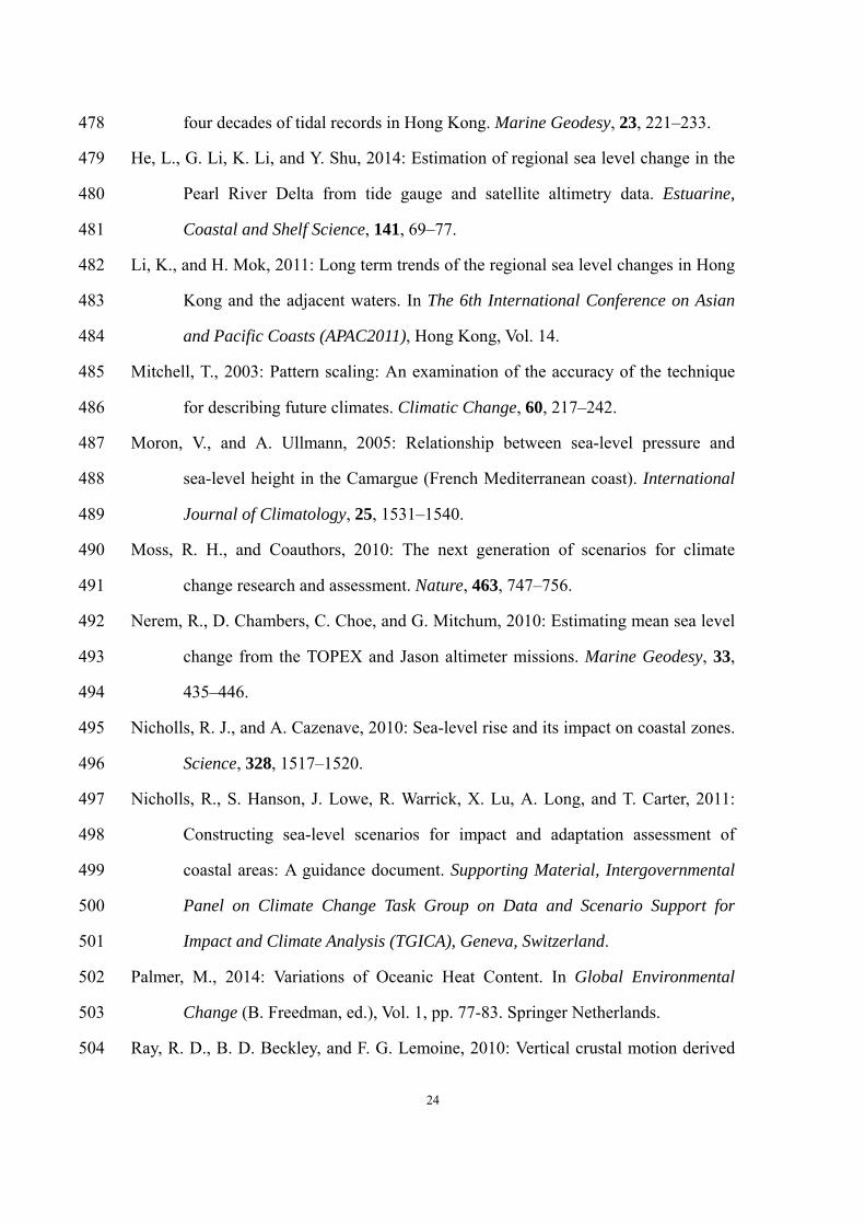
The monthly mean sea level at Macau relative to the local Chart Datum is given in

Figure 2. The Chart Datum in Macau is defined to be 1.8 m and 2.34 m below mean

sea level for the periods 1925–1966 and 1967–present, respectively. To remove the

datum discontinuity, the monthly means have been reduced to a common datum, 2.34

m below mean sea level. An overall upward trend of RSL is revealed at a rate of 1.35

mm/year. However, the rising trend is not monotonic but dominated by multidecadal

12

229

230

231

232

233

234

235

236

237

238

239

240

241

242

243

244

245

246

247

248

249

variability. From mid-1950s to 1970s, the sea level generally falls, with a linear trend

of -9.6 mm/year. Since the 1970s, the sea level in Macau has risen significantly, at a

rate of 4.2 mm/year.

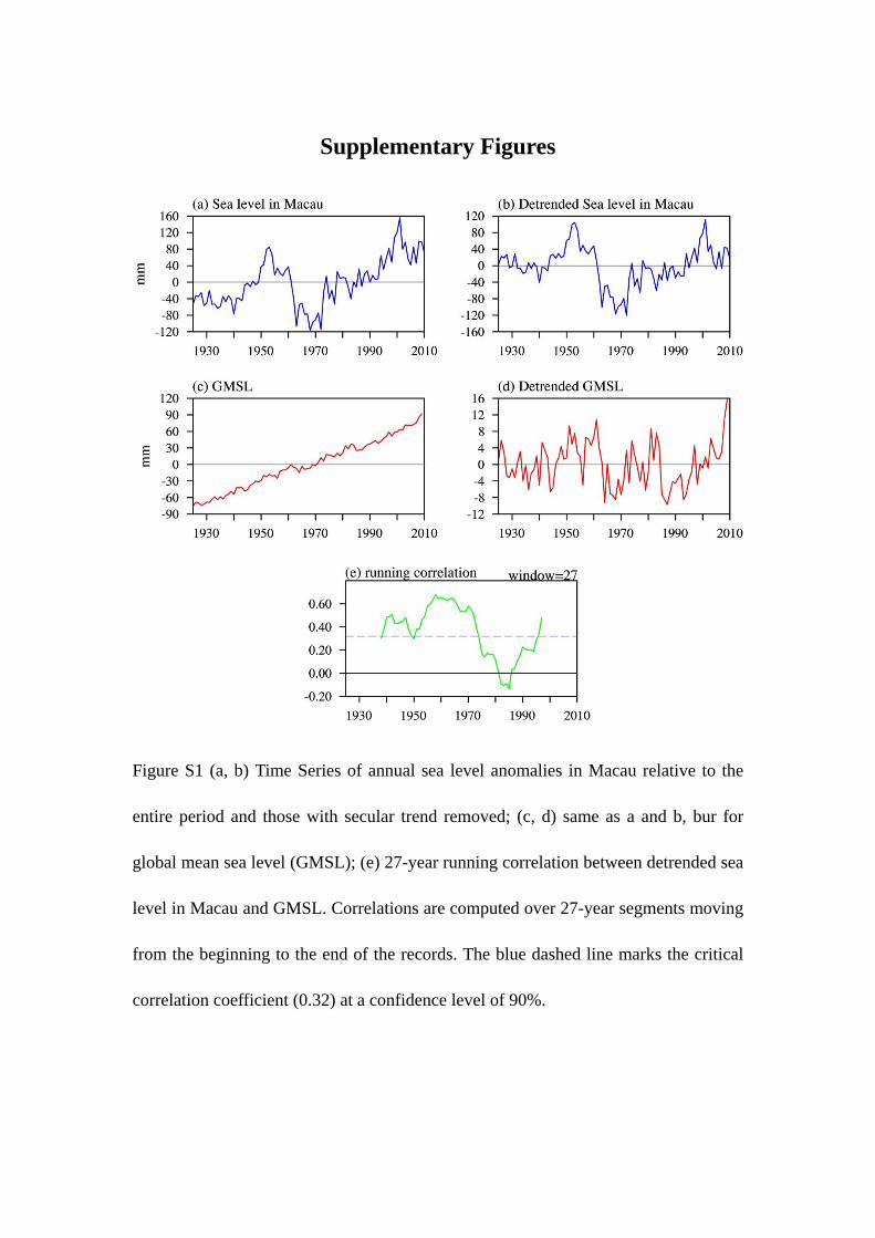
Additional Figure S1 in the supplement illuminates the possible links between sea

level changes in Macau and GMSL. Although seemingly close to linear, the evolution

of GMSL does contain decadal scale fluctuation, as illustrated in Figure S1d. It is

noticeable that the GMSL also experienced similar regime shift from the 1950s to the

early 1970s, but with weak amplitude. Further, 27-year sliding correlation shown in

Figure S1e confirms temporally consistency between detrended sea level in Macau

and GMSL before mid-1970s, suggesting that global-scale change may play a crucial

role in shaping sea level in Macau prior to mid-1970s. However, such an association

tends to break down since 1970, implying that the sea level change due to local and

regional factors dominates from mid-1970s onward. These conjectures need to be

proven through extensive diagnoses and experimentation, but it is beyond the scope of

this study to go into details.

The historical perspectives of sea water levels adjacent to Macau are next examined.

Figure S2 demonstrated the evolution of annual sea level with long-term

climatological mean removed at ZHAPO, TAI PO KAU and NORTH POINT

QUARRY BAY, which have record lengths of more than 30 years. It is noticeable that

the temporal pattern of sea level observed at ZHAPO, TAI PO KAU and NORTH

POINT QUARRY BAY are remarkably similar to that over Macau, with a rapid

13

250

251

252

253

254

255

256

257

258

259

260

261

262

263

264

265

266

267

268

269

270

declince from 1950 to around 1970 followed by general upward trend since then. The

sea levels at the three tide gauge sites are highly correlated with that for the Macau,

with correlation coefficients of 0.79, 0.69 and 0.73, respectively. Also, the sea level at

these three tide gauges rose at a rate of 2.6, 2.5 and 2 mm/year for the period 1993 to

2012, significant at 95% confidence level. On the whole, the sea level oscillations in

historical perspective are found to exhibit region-scale spatially coherent signals

across the shoreline band of SC.

From the perspective of satellite altimetry, as shown in Figure 3 (also reported by

IPCC AR5), sea level has not risen uniformly worldwide during the satellite era

(1993–2012). In some regions such as the eastern Pacific, rates of sea level change are

slower than the global average or even negative. However, the western Pacific is

characterized by pronounced greater-than-average sea level rise. This is also the case

for Macau, whose rate of SLR since 1993 amounts to 3.2 mm/year, higher than the

global mean rate of about 2.9 mm/year. Moreover, we will see in Section 5 that the

sea level at Macau will continue to rise faster than the global mean in the future.

Since VLM is essential to the local effects of SLR, the most important task is to

estimate the VLM at Macau following the procedure outlined in Section 3.1. The

monthly sea level difference, altimetry minus tide gauge, is calculated over

1993–2010. Figure 4(a) displays the monthly altimetry and tide gauge sea level at

Macau. These two time series are highly coherent, with a correlation coefficient of

0.83. The sequence of altimeter minus gauge differences is shown in Figure 4(b), with

14

271

272

273

274

275

276

277

278

280

281

282

283

284

285

286

287

288

289

290

the linear fit imposed. As indicated by the linear trend, the rate of VLM at Macau is

estimated at –0.153 mm/year, accumulating only 1.53 cm of subsidence over a span of

one century. An identical outcome can also be achieved if we rely on the annual

average time series (figure not shown). Consequently, it can be concluded that Macau

has virtually no vertical motion. Finally, it is necessary to emphasize that the tendency

of VLM is computed indirectly; if geodetic measures from GPS are launched in the

future, VLM will be estimated more accurately.

5 Future scenarios of sea level rise 279

Prior to model projections of future sea level in Macau and adjacent waters, it is

necessary to test model performance. Essentially, the state-of-art climate simulations

indeed reflect the part of variability due to long-term signals, but do not account for

interannual/decadal variability. Thus, it is more relevant to evaluate the skill of

climate models to simulate trends. Unfortunately, the downscaled outputs of historical

simulations offered by SimCLIM cover a short time span starting from 1995. With

readily available data, it is found that the observed trend for 1995-2010 falls within

the models’ range, approaching the upper bound exactly (Figure not shown), which

demonstrates their ability to capture present climate tendency during the given period.

Despite uncertainties in simulations, models are unanimous in their prediction of

substantial sea level rise at Macau under greenhouse gas increases, as we will see

15

291

292

293

294

295

296

297

298

299

300

301

302

303

304

305

306

307

308

309

310

311

below.

As clarified in Section 3.1, regional sea level change contains three contributions:

GMSL change, departures from GMSL, and VLM. First, the future projected GMSL

relative to 1986–2005 under four emission scenarios is shown in Figure 5. For each

scenario, low, medium, and high climate sensitivity projections are provided.

Generally, climate sensitivity refers to the equilibrium change in surface air

temperature following a unit change in radiative forcing. Since different GCMs

produce different results for the same greenhouse gas (GHG) emission scenarios,

GCMs have different climate sensitivities. The GMSL is expected to rise for all

emission scenarios and climate sensitivities. Furthermore, the highest sea level rise is

projected under the RCP8.5 scenario, and the lowest under the RCP2.6 scenario,

which corresponds to the highest and lowest global warming in the future. In

particular, the ranges of global SLR in 2100 are 28–61 cm, 36–71 cm, 38–73 cm, and

53–98 cm under RCP2.6, RCP4.5, RCP6.0, and RCP8.5, respectively. If we combine

emission uncertainty and climate sensitivity uncertainty, the plausible GMSL change

by 2100 ranges from 28 to 98 cm. Table 3 reports details of the GMSL changes,

including the central estimate and likely range, for 2020, 2060, and 2100. At the

beginning of this century, the magnitude of change in GMSL among different

emission scenarios is fundamentally identical, indicating the limited effect of

greenhouse gas (GHG) concentration on the response of GMSL. However, the

discrepancies in GMSL rise among different RCP scenarios become more and more

16

312

313

314

315

316

317

318

319

320

321

322

323

324

325

326

327

328

329

330

331

332

noticeable as time progresses, especially at the end of the 21st century. Finally, it is

noteworthy that the results yielded here are quite consistent with the IPCC AR5

(Church et al., 2013).

Second, regional departure from the GMSL in the scenario period is subsequently

examined. The projected scaling factors in Macau for all climate models and their

average are given in Figure 6. There is a clear consensus among models (probability >

85%) that sea level in Macau is likely to rise more rapidly than the global average,

with the maximum scaling factor of 1.76 being recorded by CNRM-CM5. The scaling

factors from HadGEM2-CC, HadGEM2-ES, and MIROC5, although less than 1, are

very close to 1. Based on the multimodel ensemble mean, the ratio of local sea level

change to the global average is 1.23, suggesting that the rate of SLR in Macau is 20%

higher than the GMSL. In addition, as indicated by Figure S3, faster sea level rise

than the ocean as a whole occupies not only just Macau but indeed all over coastal

areas along SC, with a high degree of intermodel consistency. Subsequently, what are

the driving forces behind the greater-than-average sea level rise in Macau? To address

this problem, regional thermal conditions and dynamic processes that influence

regional sea level are illuminated. Regarding local thermal conditions, Figure 7 shows

the departures of local full depth OHC changes from the global average. The ocean

along China’s coastline appears to be warming more quickly than the global average,

indicating an enhanced thermal expansion effect and thus higher sea level. In

particular, the area adjacent to Macau is characterized by much stronger intermodel

17

333

334

335

336

337

338

339

340

341

342

343

344

345

346

347

348

349

350

351

352

353

agreement, which persists through the 21st century. The inhomogeneous spatial pattern

of projected oceanic heat gain is primarily respond to changes in air-sea fluxes and

ocean circulation (Palmer et al., 2014). The downward net surface heat flux, a sum of

shortwave radiation, longwave radiation, sensible heat flux and latent heat flux,

around Macau-adjacent seawaters exhibits an evident positive trend, indicating

increased heat penetrating into the ocean (Figure not shown). Apart from the influence

of non-uniform increases in OHC, changes in regional atmospheric circulation also

play an important role in generating in situ sea level response through physical

forcing of the wind. Based on the projected meridional wind signatures shown in

Figure 8, intensified southerlies with high intermodel coherence prevail over South

China and the surrounding region, which causes future sea level rise in Macau to be

higher than the global average via the piling up of local water. Why does southerly

wind tend to strengthen in future? With the global warming, the temperature increase

over land will be more rapid than that over the oceans, and the continental-scale

land-sea thermal contrast will become larger in summer and smaller in winter.

Therefore, it follows that the summer monsoon will be stronger and the winter

monsoon weaker in the future, promoting intensified southerly anomalies (Ding et al.,

2010). In short, faster sea level rise in Macau is connected with a stronger thermal

expansion of local sea water and strengthened southerlies in the future.

The last component essential to creating an RSL rise scenario is the VLM-related

trends. In Macau, however, the VLM makes little contribution to RSL change. Figure

18

354

355

356

357

358

359

360

361

362

363

364

365

366

367

368

369

370

371

372

373

374

9 and Figure 10 illuminate the projected change in ASL and RSL (ASL combined with

VLM), respectively. There is obviously high agreement between ASL and RSL, so in

the following investigation we focus mainly on RSL (Figure 10), which is the ultimate

objective in this study. Despite the sea level in Macau tracking close to the global

average (Figure 5) throughout the entire 21st century, its amplitude is stronger. If we

consider the worst-case RCP8.5 together with high climate sensitivity, for instance,

sea level in Macau will rise by 118 cm, 20 cm above the global mean. The values

associated with the projected SLR in Macau are shown in Table 4. Based on Figure 10

and Table 4, three basic characteristics can be identified: (1) The higher emission

scenario leads to a more remarkable sea level rise than the lower emission scenario:

90 cm under RCP8.5 versus 54 cm under RCP4.5 by 2100, for example, as a

consequence of stronger ocean thermal expansion and loss of mass from glaciers and

ice sheets due to more rapid warming. Moreover, under RCP8.5 the linear trends for

the periods 2020–2060 and 2060–2100 are 0.75 mm/year and 1.25 mm/year,

respectively, highlighting the accelerating SLR in the future, which is also the case for

RCP6.0. However, under RCP2.6 and RCP4.5, the SLR will remain at a moderate and

steady rate. (2) The different emission scenarios do not lead to dramatically different

sea level responses during the beginning of the 21st century, but thereafter the

projections begin to diverge. As shown in Table 4, all emission scenarios predict a sea

level rise of 10 cm, with a probable range from 8 cm to 12 cm, by 2020; however, by

2100 the projected sea levels under RCP8.5 reach 53–98 cm, double those under

19

375

376

377

378

379

380

381

382

383

384

385

386

387

389

390

391

392

393

394

RCP2.6. (3) The climate-sensitivity-related uncertainty tends to broaden with time,

since the full ranges for 2020, 2060, and 2100 under RCP4.5 are 4 cm, 19 cm, and 42

cm, respectively. In contrast, given the same climate sensitivity, the random

uncertainty bounds are rather narrow, as indicated by the shading in Figure 10.

Consequently, the majority of the uncertainty originates from poor knowledge of

climate sensitivity along with emission level, whereas other factors are likely to be

secondary.

In short, the SLR in Macau by 2100 will span between a minimum of 35 cm and a

maximum of 118 cm, depending on the emission scenario and climate sensitivity. In

addition, CMIP5 simulations give analogous patterns and magnitudes of future sea

level rise along the entire SC coasts compared to the changes in Macau, and will not

be detailed here.

6 Conclusions 388

Global warming–related SLR constitutes a substantial threat to Macau, due to its

low elevation, small size, and ongoing land reclamation. This study is devised to

determine the long-term variation of sea level change in Macau, as well as to develop

future scenarios based on tide gauge and satellite data and GCM simulations, aiming

to provide knowledge for SLR mitigation and adaptation.

Based on local tide gauge records, the rate of SLR shifts from about 1.35 mm/year

20

395

396

397

398

399

400

401

402

403

404

405

406

407

408

409

410

411

412

413

414

415

over 1925–2010 to 4.2 mm/year over 1970–2010, reflecting an apparent acceleration

of SLR. Despite the overall upward trend, the sea level in Macau also exhibits decadal

variability. Satellite altimetry data furthermore reveal that the sea level near Macau is

rising 10% faster than the global mean during the period from 1993 to 2012. Since the

local sea level could be significantly adjusted by the rate of vertical land movement,

we subsequently derive it by calculating the linear trend of sea level difference

between satellite altimetry and tide gauge measurement. The result indicates that there

is almost no rising or sinking of the landmass in Macau. However, complementary

measurements based on high-accuracy GPS equipment co-located with the tide gauge

at Macau should be implemented in the future to better monitor the rate of VLM.

As projected by a suite of climate models, the Macau SLR deviates positively from

the global average by about 20%, indicating a 1.2 m SLR in Macau, corresponding to

a unit increase of global average SLR. This is induced primarily by a

greater-than-average rate of oceanic thermal expansion in Macau, together with

enhanced southerly anomalies that lead to a piling up of sea water. Specifically,

relative sea levels with the local rate of VLM added indicate a rise of 8–12, 22–51,

and 35–118 cm by 2020, 2060, and 2100 with respect to the 1986–2005 baseline

climatology, respectively, with the amount of rise dependent on the emission scenario

and climate sensitivity. If we consider the medium emission scenario RCP4.5 along

with medium climate sensitivity, Macau can expect to experience a SLR of 10, 34,

and 65 cm by 2020, 2060, and 2100; if the worst case happens (RCP8.5 plus high

21

416

417

418

419

420

421

422

423

424

425

426

427

428

429

430

431

432

433

434

435

436

climate sensitivity), the SLR will be far higher than that in the medium case, namely

13, 51, and 118 cm by 2020, 2060, and 2100. The SLR under the lower emission

scenario is expected to be less severe than that under higher emission scenarios: by

2100, an SLR of 53–98 cm in Macau, almost twice as fast as that under RCP2.6.

Moreover, the SLR will accelerate under RCP6.0 and RCP8.5, while remaining at a

moderate and steady rate under RCP4.5 and RCP2.6. The GHG forcing scenario has

virtually no influence on the projected change during the beginning of this century,

but its impact on divergent sea level responses becomes noticeable after midcentury.

The majority of the projection uncertainty comes from the emission scenario and poor

knowledge of climate sensitivity. By 2020, the uncertainty range is only 4 cm, yet by

2100 the range will be increased to 83 cm. Moreover, the sea level changes in the past

and future over the whole of SC to a large extent resemble that in Macau.

This study concerns scenario development, which is only the first step in the whole

process. Additional problems need to be addressed, as follows: (1) Given the large

uncertainties in future projections, the obvious question is how to select appropriate

SLR values. Consequently, continuous monitoring of actual SLR, and understanding

of which emission scenario and climate sensitivity is the most realistic, are essential to

the scenario choice. (2) Extreme high-water events (short-term phenomena) in Macau

are not examined in this study, but they must be recognized in impact analysis.

Although rising sea level will increase the probability of storm surges and waves,

quantitative assessments of such risks are inevitable in the future. (3) Last but not

22

437

438

439

440

441

442

443

444

445

446

447

448

449

450

least, what are the most suitable adaptation policies and planning objectives in Macau?

In general, we need to combine the consequences of SLR and the potential costs

incurred in future adaptations. Therefore, feasible mitigation and adaptation strategies

should be initiated to address SLR.

Acknowledgement

We thank the Working Group on Coupled Modeling of the World Climate Research

Program for sponsoring CMIP5 and the climate modeling groups for producing and

making the model output available, and we acknowledge CLIMsystems for providing

SimCLIM software. This work was supported by National Basic Research Program of

China 2012CB955600 (2012CB955601 ， 2012CB955602 ， 2012CB955603 ，

2012CB955604) and National Science Fund for Distinguished Young Scholars

41425019.

23

452

453

454

455

456

457

458

459

460

461

462

463

464

465

466

467

468

469

470

471

472

473

474

475

476

477

7 References 451

Cazenave, A., K. Dominh, F. Ponchaut, L. Soudarin, J. F. Cretaux, and C. Le Provost,

1999: Sea level changes from Topex-Poseidon altimetry and tide gauges, and

vertical crustal motions from DORIS. Geophysical Research Letters, 26,

2077–2080.

Chen, D., and A. Omstedt, 2005: Climate-induced variability of sea level in

Stockholm: Influence of air temperature and atmospheric circulation.

Advances in Atmospheric Sciences, 22, 655–664.

Church, J. A., and N. J. White, 2006: A 20th century acceleration in global sea-level

rise. Geophysical Research Letters, 33, L01602.

Church, J. A., and N. White, 2011: Sea-level rise from the late 19th to the rarly 21st

century. Surveys in geophysics, 32, 585-602.

Church, J.A., and Coauthors, 2013: Sea Level Change. In: Stocker, T.F., and

Coauthors (eds.), Climate Change 2013: The Physical Science Basis.

Contribution of Working Group I to the Fifth Assessment Report of the

Intergovernmental Panel on Climate Change. Cambridge University Press,

Cambridge, United Kingdom and New York, NY, USA.

Dibarboure, G., O. Lauret, F. Mertz, V. Rosmorduc, and C. Maheu, 2014:

SSALTO/DUACS user handbook: (M) SLA and (M) ADT near-real time and

delayed time products. Rep. CLS‐DOS‐NT, 6, 39.

Ding, X., D. Zheng, Y. Chen, J. Chao, and Z. Li, 2001: Sea level change in Hong

Kong from tide gauge measurements of 1954–1999. Journal of Geodesy, 74,

683–689.

García, D., I. Vigo, B. F. Chao, and M. C. Martínez, 2007: Vertical crustal motion

along the Mediterranean and Black Sea coast derived from ocean altimetry

and tide gauge data. Pure and Applied Geophysics, 164, 851–863.

Baki Iz H., C. K. Shum, 2000: Mean sea level variation in the South China Sea from

24

478

479

480

481

482

483

484

485

486

487

488

489

490

491

492

493

494

495

496

497

498

499

500

501

502

503

504

four decades of tidal records in Hong Kong. Marine Geodesy, 23, 221–233.

He, L., G. Li, K. Li, and Y. Shu, 2014: Estimation of regional sea level change in the

Pearl River Delta from tide gauge and satellite altimetry data. Estuarine,

Coastal and Shelf Science, 141, 69–77.

Li, K., and H. Mok, 2011: Long term trends of the regional sea level changes in Hong

Kong and the adjacent waters. In The 6th International Conference on Asian

and Pacific Coasts (APAC2011), Hong Kong, Vol. 14.

Mitchell, T., 2003: Pattern scaling: An examination of the accuracy of the technique

for describing future climates. Climatic Change, 60, 217–242.

Moron, V., and A. Ullmann, 2005: Relationship between sea-level pressure and

sea-level height in the Camargue (French Mediterranean coast). International

Journal of Climatology, 25, 1531–1540.

Moss, R. H., and Coauthors, 2010: The next generation of scenarios for climate

change research and assessment. Nature, 463, 747–756.

Nerem, R., D. Chambers, C. Choe, and G. Mitchum, 2010: Estimating mean sea level

change from the TOPEX and Jason altimeter missions. Marine Geodesy, 33,

435–446.

Nicholls, R. J., and A. Cazenave, 2010: Sea-level rise and its impact on coastal zones.

Science, 328, 1517–1520.

Nicholls, R., S. Hanson, J. Lowe, R. Warrick, X. Lu, A. Long, and T. Carter, 2011:

Constructing sea-level scenarios for impact and adaptation assessment of

coastal areas: A guidance document. Supporting Material, Intergovernmental

Panel on Climate Change Task Group on Data and Scenario Support for

Impact and Climate Analysis (TGICA), Geneva, Switzerland.

Palmer, M., 2014: Variations of Oceanic Heat Content. In Global Environmental

Change (B. Freedman, ed.), Vol. 1, pp. 77-83. Springer Netherlands.

Ray, R. D., B. D. Beckley, and F. G. Lemoine, 2010: Vertical crustal motion derived

25

505

506

507

508

509

510

511

512

513

514

515

516

517

518

519

520

521

522

523

524

525

526

527

528

529

from satellite altimetry and tide gauges, and comparisons with DORIS

measurements. Advances in Space Research, 45, 1510–1522.

Santer, B. D., T. M. L. Wigley, M. E. Schlesinger, and J. F. B. Mitchell, 1990:

Developing climate scenarios from equilibrium GCM results. MPI report

number 47, Hamburg.

Stephens, S. A., and R. G. Bell, 2009: Review of Nelson City minimum ground level

requirements in relation to coastal inundation and sea-level rise.

HAM2009-124, National Institute of Water and Atmospheric Research. 58 pp

Sun, Y., and Y. Ding, 2010: A projection of future changes in summer precipitation

and monsoon in East Asia. Science China Earth Sciences, 53, 284-300.

Taylor, K. E., R. J. Stouffer, and G. A. Meehl, 2012: An overiew of CMIP5 and the

experiment design. Bulletin of the American Meteorological Society, 93,

485–498.

Walsh, K., 1998: Global warming and sea level rise on the Gold Coast. Report

Prepared for the Gold Coast City Council, Mordialloc, Australia, CSIRO

Atmospheric Research. 34pp.

Warrick, R. A., W. Ye, P. Kouwenhoven, J. Hay, and C. Cheatham, 2005: New

developments of the SimCLIM model for simulating adaptation to risks

arising from climate variability and change. In Zerger, A. and R. M. ARGENT,

(Eds.) MODSIM 2005. Proceedings of the International Congress on

Modelling and Simulation. Canberra, Australia; Modelling and Simulation

Society of Australia and New Zealand. 170-176.

Wong, W., K. Li, and K. Yeung, 2003: Long term sea level change in Hong Kong.

Hong Kong Meteorological Society Bulletin, 13, 24–40.

26

530

531

Table 1 Tide gauge stations along the SC used for this study, their latitude- longitude

location and record periods.

Station Name Latitude(°N)

Longitude(°E)record period Data Source

Macau 22.2

113.55 1925-2010

Macau

Meteorological

and Geophysical

Bureau

ZHAPO 21.583

111.817 1959 – 2014 PSMSL

TAI PO KAU 22.443

114.184 1963 – 2013 PSMSL

NORTH POINT/QUARRY BAY 22.291

114.213 1950 – 2013 PSMSL

532

533

534

535

27

536 Table 2 Summary of 24 climate models from CMIP5 used in this study

Model Modeling Center

bcc-csm1-1 Beijing Climate Center, China Meteorological

Administration bcc-csm1-1-m

CanESM2 Canadian Centre for Climate Modelling and Analysis

CCSM4 National Center for Atmospheric Research

CMCC-CMS Centro Euro-Mediterraneo per i Cambiamenti Climatici

CMCC-CM

CNRM-CM5

Centre National de Recherches Météorologiques / Centre

Européen de Recherche et Formation Avancée en Calcul

Scientifique

CSIRO-Mk3-6-0

Commonwealth Scientific and Industrial Research

Organization in collaboration with Queensland Climate

Change Centre of Excellence

GFDL-CM3

NOAA Geophysical Fluid Dynamics Laboratory GFDL-ESM2G

GFDL-ESM2M

GISS-E2-R-CC NASA Goddard Institute for Space Studies

GISS-E2-R

HadGEM2-CC Met Office Hadley Centre (additional HadGEM2-ES

28

realizations contributed by Instituto Nacional de Pesquisas

Espaciais)

HadGEM2-ES

inmcm4 Institute for Numerical Mathematics

MIROC5

Atmosphere and Ocean Research Institute (The University

of Tokyo), National Institute for Environmental Studies,

and Japan Agency for Marine-Earth Science and

Technology

MIROC-ESM Japan Agency for Marine-Earth Science and Technology,

Atmosphere and Ocean Research Institute (The University

of Tokyo), and National Institute for Environmental StudiesMIROC-ESM-CHEM

MPI-ESM-LR Max-Planck-Institut für Meteorologie (Max Planck Institute

for Meteorology) MPI-ESM-MR

MRI-CGCM3 Meteorological Research Institute

NorESM1-M Norwegian Climate Centre

NorESM1-ME

537

538

539

29

540

541

Table 3 Central estimate and range of GMSL change (cm) relative to 1986–2005

climatology under four emission scenarios (RCP2.6, RCP4.5, RCP6.0, and RCP8.5)*

2020 2060 2100

RCP2.6 8 (6-10) 26 (18-35) 44 (28-61)

RCP4.5 8 (6-10) 28 (21-37) 53 (36-71)

RCP6.0 8 (6-10) 27 (19-35) 55 (38-73)

RCP8.5 8 (6-11) 33 (24-42) 74 (53-98)

* Results are presented for each emission scenario. Values are the central estimate

with the range in the parentheses. The projected changes in the case of medium, low,

and high climate sensitivities are adopted as the central estimate, lower, and upper

bounds of the range.

542

543

544

545

546

547

30

548 Table 4 The same as Table 3, but for Macau (unit: cm)

2020 2060 2100

RCP2.6 10 (8-12) 32 (22-43) 54 (35-74)

RCP4.5 10 (8-12) 34 (26-45) 65 (44-86)

RCP6.0 10 (8-12) 33 (24-43) 67 (47-88)

RCP8.5 10 (8-13) 40 (30-51) 90 (65-118)

549

550

Figure 1 Geographical location of Macau (red dot) along with ZHAPO, TAI PO

KAU and North Point/Quarry Bay (NPQB) (brown dots) in China

31

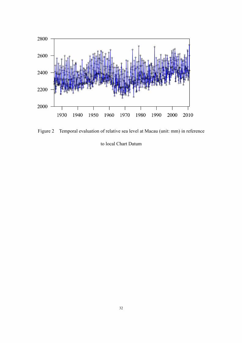
Figure 2 Temporal evaluation of relative sea level at Macau (unit: mm) in reference

to local Chart Datum

32

Figure 3 Spatial pattern in sea level trends (unit: mm/year) for the period 1993 to

2012 based on AVISO

33

Figure 4 (Top) altimetric (blue dashes) and tide gauge (red solid) sea level

anomalies at Macau from 1993 to 2010 at monthly intervals, and (bottom) their

difference (green dots) along with the fitted linear regression (blue line).

34

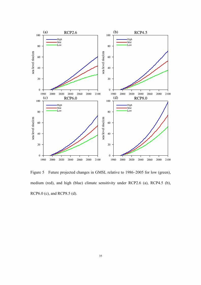
Figure 5 Future projected changes in GMSL relative to 1986–2005 for low (green),

medium (red), and high (blue) climate sensitivity under RCP2.6 (a), RCP4.5 (b),

RCP6.0 (c), and RCP8.5 (d).

35

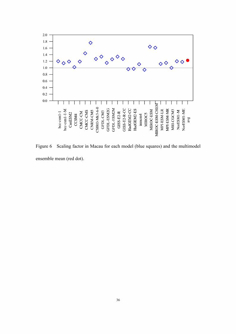
Figure 6 Scaling factor in Macau for each model (blue squares) and the multimodel

ensemble mean (red dot).

36

Figure 7 Spatial pattern of the departure of local OHC change from the global

average (unit: °C) for 2010–2039 (top row), 2040–2069 (middle row), and 2070–2099

(bottom row) under RCP4.5 (left column) and RCP8.5 (right column). Stippling

indicates where at least 75% of all GCMs agree on the sign. Red implies a faster rate

of OHC increase compared to the global average, while blue denotes the opposite.

37

38

Figure 8 Spatial pattern of meridional wind change at 1000 hPa (unit: m/s) from the

reference period (1986–2005) to 2010–2039 (top row), 2040–2069 (middle row), and

2070–2099 (bottom row) under RCP4.5 (left column) and RCP8.5 (right column).

Stippling indicates where at least 75% of all GCMs agree on the sign. Cyan indicates

39

southerly anomalies, while brown indicates the opposite.

Figure 9 The same as Figure 5, but for absolute sea level rise at Macau. Shading

denotes the interquartile range across all climate models.

40

Figure 10 The same as Figure 9, but for relative sea level rise (incorporating VLM)

at Macau.

41

Supplementary Figures

Figure S1 (a, b) Time Series of annual sea level anomalies in Macau relative to the

entire period and those with secular trend removed; (c, d) same as a and b, bur for

global mean sea level (GMSL); (e) 27-year running correlation between detrended sea

level in Macau and GMSL. Correlations are computed over 27-year segments moving

from the beginning to the end of the records. The blue dashed line marks the critical

correlation coefficient (0.32) at a confidence level of 90%.

Figure S2 Annual sea level anomalies at ZHAPO(a), TAI PO KAU(b), NORTH

POINT QUARRY BAY(c) from 1950 to 2014. Red dashed line denotes the linear

trend over the period of 1993 to 2012.

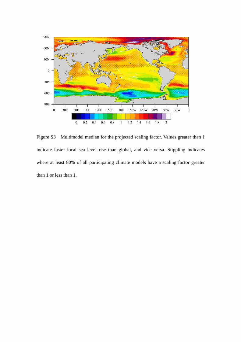
Figure S3 Multimodel median for the projected scaling factor. Values greater than 1

indicate faster local sea level rise than global, and vice versa. Stippling indicates

where at least 80% of all participating climate models have a scaling factor greater

than 1 or less than 1.