Hiring insiders or outsiders to the firm and its effect on ...
25
Hiring insiders or outsiders to the firm and its effect on accounting system choice November 2019 preliminary comments are welcome Barbara Schöndube-Pirchegger Otto-von-Guericke-University Magdeburg Faculty of Economics and Management PO-Box 4120 D - 39016 Magdeburg [email protected] phone:+49-391-67-58728 Abstract: In this paper we investigate whether it is more favorable for a firm to offer an open management position to an insider or to hire someone from outside the firm. The insider is assumed to hold private information about the working environment, such as specific characteristics and challenges of the job. An applicant from outside the firm, in contrast, does not hold any superior knowledge. Rather, he possesses the same information and holds the same expectations as the principal in charge of hiring. On top of the hiring choice, the firm has some discretion with regard to the accounting system to be implemented. The more rigid the system the more expensive earnings management/window dressing activities become for the manager. We analyze both choice problems individually as well as possible interrelations. We find that it is optimal for the principal to hire a manager from outside the firm when alternative working environments are not too distinct. Otherwise, he would prefer an insider. With regard to the accounting system effect, our analysis shows that a more rigid system is always preferred to a less rigid one if an outsider is hired. If the firm hires an insider, however, this is no longer the case. Our results show that opting for a more rigid accounting system can be both, favorable or detrimental, depending on the specifics of the agency problems in place.
Transcript of Hiring insiders or outsiders to the firm and its effect on ...
Hiringinsidersoroutsiderstothefirmanditseffectonaccountingsystemchoice
November 2019
preliminary
comments are welcome
Barbara Schöndube-Pirchegger
Otto-von-Guericke-University Magdeburg Faculty of Economics and Management PO-Box 4120 D - 39016 Magdeburg [email protected] phone:+49-391-67-58728
Abstract:
In this paper we investigate whether it is more favorable for a firm to offer an open management position to an
insider or to hire someone from outside the firm. The insider is assumed to hold private information about the
working environment, such as specific characteristics and challenges of the job. An applicant from outside the
firm, in contrast, does not hold any superior knowledge. Rather, he possesses the same information and holds
the same expectations as the principal in charge of hiring.
On top of the hiring choice, the firm has some discretion with regard to the accounting system to be
implemented. The more rigid the system the more expensive earnings management/window dressing activities
become for the manager.
We analyze both choice problems individually as well as possible interrelations.
We find that it is optimal for the principal to hire a manager from outside the firm when alternative working
environments are not too distinct. Otherwise, he would prefer an insider. With regard to the accounting system
effect, our analysis shows that a more rigid system is always preferred to a less rigid one if an outsider is hired.
If the firm hires an insider, however, this is no longer the case. Our results show that opting for a more rigid
accounting system can be both, favorable or detrimental, depending on the specifics of the agency problems in
place.
2
1. Introduction
When a management position needs to be filled, firms in general face two alternatives. They can
promote an ambitious candidate from inside the firm or they can offer the job to an external applicant.
Both alternatives are commonly used in firms. With regard to the special case of US CEO appointments,
it seems that outside appointments became more popular over time. As reported in Murphy (2013)
the percentage of outside appointments increased from 15% in the 1970s to roughly a third at the end
of the century.1
Even though external versus internal hiring is likely to differ with respect to various aspects, an
important one is different information endowment of the applicants. A candidate that already holds a
position within the firm is probably well informed about the firm’s processes, the work climate, the
firm’s specifics, latest developments, and what to expect from the new position. Such information is
not available to an external candidate nor to (external) directors or compensation committee members
in charge of hiring a manager.
We focus on these differences in information endowment when analyzing whether it benefits the
principal to hire an outsider or an insider. Obviously, the insider holds private information that
facilitates decision making. However, he can exploit this knowledge for his private benefit and at the
expense of the principal. In contrast, an uninformed manager cannot exploit any informational
advantage, but suffers from poorer choices due to lack of information.
In terms of the model we use, hiring an outside manager results in a moral hazard problem. Ex ante
both parties to the contract, principal and agent, are symmetrically informed but the agent performs
a private work effort in our model. If, in contrast, an internal applicant is hired, an adverse selection
problem and moral hazard problem are present simultaneously. The agent holds private pre contract
information and can use them to extract rents from the principal.
Along with the hiring choice, we model some discretion with regard to the accounting system to be
implemented within the firm. Keeping the model simple, we assume that accounting systems that are
more rigid increase the manager’s cost related to a window dressing activity. We investigate which
accounting system to choose and whether this choice is related to the hiring decision. Implementation
costs as well as costs of operating the system are neglected throughout the analysis.
We find that the choice of hiring an outsider versus an insider critically depends on the degree of
uncertainty present with regard to the type of working environment within the firm. If possible working
environments are no too distinct, the principal prefers to hire an uninformed outside manager. Beyond
some threshold hiring an insider becomes the better choice.
With regard to the accounting system it turns out that once an outsider is hired, a more rigid
accounting system is always preferred to a less rigid one. As a consequence, the principal goes for the
most rigid system available. If an insider is hired, this is not necessarily the case but depends on the
magnitude of the adverse selection problem. If the adverse selection problem is sufficiently strong, a
more rigid accounting system decreases the principal’s welfare as compared to a less rigid one, in
general or at least within some range.
1 See Murphy (2013), p.331f.
3
2. Relatedliterature
Our paper studies whether a principal benefits mostly from hiring an informed or an uninformed
manager. Formally, we juxtapose a moral hazard type agency problem and one of joint moral hazard
and adverse selection. In both settings, the agent performs two unobservable efforts, a productive one
and a window dressing activity. The cost of the latter is affected by the accounting system in place.
Given these inputs, our model somewhat builds on the classical literature on moral hazard, e.g.
Holmström (1979), Grossmann and Hart (1983), and Holmström and Milgrom (1991), and on the
literature on multi‐task problems such as Feltham and Xie (1994). It is also related to the adverse
selection literature e.g. Laffont and Tirole (1993) and Rajan and Saouma (2006), and the joint moral
hazard and adverse selection literature, e.g. Sappington (1984) and Melumad and Reichelstein (1989).
As the manager performs a window dressing activity that is restricted by a rigid accounting system,
further ties exist to the literature on earnings management, e.g. Dye (1988), Demski (1998) and Arya,
Glover, and Sunder (1998), and on effects of tighter accounting standards, e.g. Ewert and Wagenhofer
(2005).
A paper that is closely related to our work is Rajan and Saouma (2006). In their paper a manager
performs several tasks that affect the principal’s payoffs. Different types of risk neutral managers differ
in disutility related to performing each task as in our model. Rather than to learn his type, however,
the manager in Rajan/Saouma receives a signal that is informative about his type before he signs the
contract and chooses his effort. They allow for a continuum of informational states ranging from
perfectly informative to perfectly uninformative. Moreover, in their paper the principal’s payoff is
contractible and used as a performance measure. As a consequence, the congruity problem arising in
our paper is absent in Rajan/Saouma. They find that the principal’s expected net payoff is decreasing
and convex in the extent of information asymmetry. It follows that either a perfectly informed manager
or a perfectly uninformed manager is optimal. If the agent’s types are not very distinct an uninformed
manager is preferred. This result somewhat resembles the one we obtain in our two‐type setting.
Also close to our model is the paper by Beyer, Guttman, and Marinovic (2014). They consider a joint
adverse selection and moral hazard problem where an agent performs a productive effort and a
window dressing activity. Firm value is non‐contractible and earnings is the only performance measure
available for contracting. The agent is privately informed about his type. Types differ with regard to
their disutility of effort. Thus, they use a very similar model setup as we do in our paper. Even a pure
moral hazard problem is analyzed in their paper to serve as a benchmark. In contrast to our paper,
however, both, the principal and the agent are assumed to know the agent’s type in this benchmark
setting. The moral hazard problem therefore is coupled with superior information in their paper but
comes along with reduced information in ours. Consequently, and in contrast to our results, their moral
hazard setting is preferable in terms of the principal’s payoffs to the joint problem. Moreover, Beyer
et al focus on a research question quite different from ours as they are interested in the shape of the
optimal compensation contract and the effects that the agent’s ability to manipulate earnings
has on this shape.
Finally, the paper by Marinovic and Povel (2017) is related to our work as it studies the
contracting choice of a principal in a joint moral hazard and adverse selection setting which
allows for misreporting. The main distinction from our paper is that Marinovic/Povel assume
that firms compete for talented managers. They find that competition results in increased

4
incentives. Therefore, it corrects inefficiently low incentives resulting in adverse selection
settings due to downward distorted incentives for bad types. However, in the presence of
misreporting, competition may also lead to severe over‐incentives. Marinovic/Povel juxtapose the
inefficiencies related to the agency problem with and without competition and identify conditions
under which competition for talent either benefits or harms the principal.
3. The model
We consider a one shot game between a principal and an agent. The principal aims at maximizing firm
value. In order to motivate the agent to work hard, he offers an incentive contract at the beginning of
the game. We assume, however, that firm value itself is un‐contractible and thus the principal has to
revert to a contractible performance measure. This measure is affected by two types of efforts, each
performed privately by the agent. The first effort is a productive effort in the sense that it increases
firm value along with the performance measure. The second effort, in contrast, increases the
performance measure only and can be referred to as a window dressing activity.2 If the agent accepts
the contract, he provides both efforts and is paid according to his contract at the end of the game.
The performance measure y is defined as follows:
refers to the productive effort and is window dressing. , 1,2 depict the sensitivity of the performance measure with regard to both efforts.
For simplicity, we assume that firm value increases in at a similar rate as does, such that
.
Both, the principal and the agent are risk neutral.
The agent maximizes expected pay less disutility from working hard. We assume that two scenarios
exist with regard to the amount of disutility from effort the agent suffers from.
If the working environment at the firm is good, the agent faces a relatively low disutility when providing
effort. With regard to the productive effort, disutility in the presence of the good environment is
characterized by , and 0. In the bad environment, in contrast, disutility is higher and denoted
and ∆ with ∆ 0.
The agent’s disutility on the window dressing activity, however, is not only affected by the working
environment, characterized by , , , but also by the accounting system in place. To reflect that,
we presume that a rigid system imposes an extra cost on the window dressing activity that is absent
for productive effort. The extra cost possibly differs, however, depending on the type of environment.
If the working environment the agent faces is good, disutility from the window dressing effort equals
. In a bad environment, it equals ∆
. To achieve increased disutility for window
2 See e.g. Feltham/Xie (1994) or Goldman/Slezak (2006) for a similar interpretation.

5
dressing as opposed to productive effort we assume that 1and 1. We do not
predetermine, however, whether > or v.v.
Note that the presence of a good and bad environment can be interpreted in terms of two different
types of agents. The good type faces a lower disutility and the bad type a higher one. We will use this
interpretation interchangeably with the good and bad environment whenever convenient in what
follows.
Summing up, total disutility in each environment is characterized by
in the good setting and
∆ ∆
in the bad one.
The underlying rationale for the above expressions is as follows: reflects a basic effect the
accounting system has on the cost of window dressing that is common in each environment. , in
contrast, depicts an “extra” cost effect that aggravates the additional disutility the agent faces in a bad
environment. Note that this setup is carefully chosen in order to ensure several properties we consider
important: First, it makes sure that the presence of a rigid accounting system renders window dressing
more expensive no matter which environment is present. Second, disutility in the bad environment is
always larger than in the good environment. Third, in the extreme case where both our settings
integrate into a single one, disutility becomes identical as well. In other words if ∆→ 0, the disutility is the same in both expressions as it should be.
With the above specifications in place, we are ready to model the consequences of internal versus
external hiring. As stated above, we assume that both alternatives differ with regard to the information
endowment of the agent.
If an external applicant is hired, we assume that the agent does not know whether the working
environment at the firm is good or bad when he signs the contract. Thus, private information of the
agent is limited to post contract information about effort choice. With regard to the working
environment, we assume that both, agent and principal, share a common probability distribution for
each environment to be present. We denote the probability for a good working environment to be
present as and thus a bad one occurs with probability 1 .The agency problem at hand is a
(pure) moral hazard problem.
If an insider is hired instead, we assume that he is aware of the type of environment he faces when he
accepts the contract. The principal does not have such knowledge. Thus, pre‐ and post‐contracting
information asymmetry is present simultaneously, tantamount to an adverse selection problem on top
of the moral hazard problem described above.
In what follows we analyze the hiring choice problem and consider a particular accounting system as
unique to the two settings and given. We begin analyzing the poorer informational setting. The
principal hires an uninformed manager resulting in a pure moral hazard problem. In section 5 solutions
to the joint moral hazard and adverse selection setting are derived.

6
4. Optimalcontractsifanuninformedmanagerishired
In this setting, the principal hires an outsider. Neither the principal nor the agent know which working
environment is present. The principal offers an incentive contract that specifies some
performance level to be achieved by the agent. If the agent reaches the required performance level,
he receives a payment. Otherwise, he endures negative consequences .
∗ ∗
can be regarded as some kind of penalty or even dismissal due to failure. It is assumed to be
sufficiently unattractive to ensure that the manager always prefers to perform and to obtain ∗ ,
rather than . Given this contract, the agent chooses his efforts minimizing expected costs for
achieving the required performance measure value ∗.
As the agent does not know the type of working environment, expected disutility equals
,
with 1 and 1 ∆
and the agent’s optimization problem can be stated as follows.
min,
s.t. ∗.
Solving the problem we obtain ∗∗
and ∗∗
.
Given the agent’s conditionally optimal choice of effort, the principal chooses in order to maximize
his objective function
max∗
∗
s.t. ∗ 0
∗
∗
Solving the problem results in ∗
7
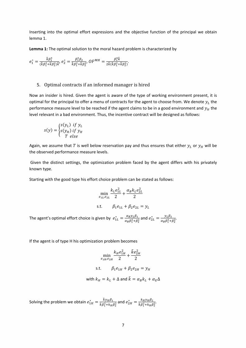
Inserting into the optimal effort expressions and the objective function of the principal we obtain
lemma 1.
Lemma 1: The optimal solution to the moral hazard problem is characterized by
∗ , ∗ , .
5. Optimalcontractsifaninformedmanagerishired
Now an insider is hired. Given the agent is aware of the type of working environment present, it is
optimal for the principal to offer a menu of contracts for the agent to choose from. We denote the
performance measure level to be reached if the agent claims to be in a good environment and the
level relevant in a bad environment. Thus, the incentive contract will be designed as follows:
Again, we assume that is well below reservation pay and thus ensures that either or will be
the observed performance measure levels.
Given the distinct settings, the optimization problem faced by the agent differs with his privately
known type.
Starting with the good type his effort choice problem can be stated as follows:
min, 2 2
s.t.
The agent’s optimal effort choice is given by ∗ and ∗ .
If the agent is of type H his optimization problem becomes
min, 2 2
s.t.
with ∆ and ∆
Solving the problem we obtain ∗ and ∗ .
8
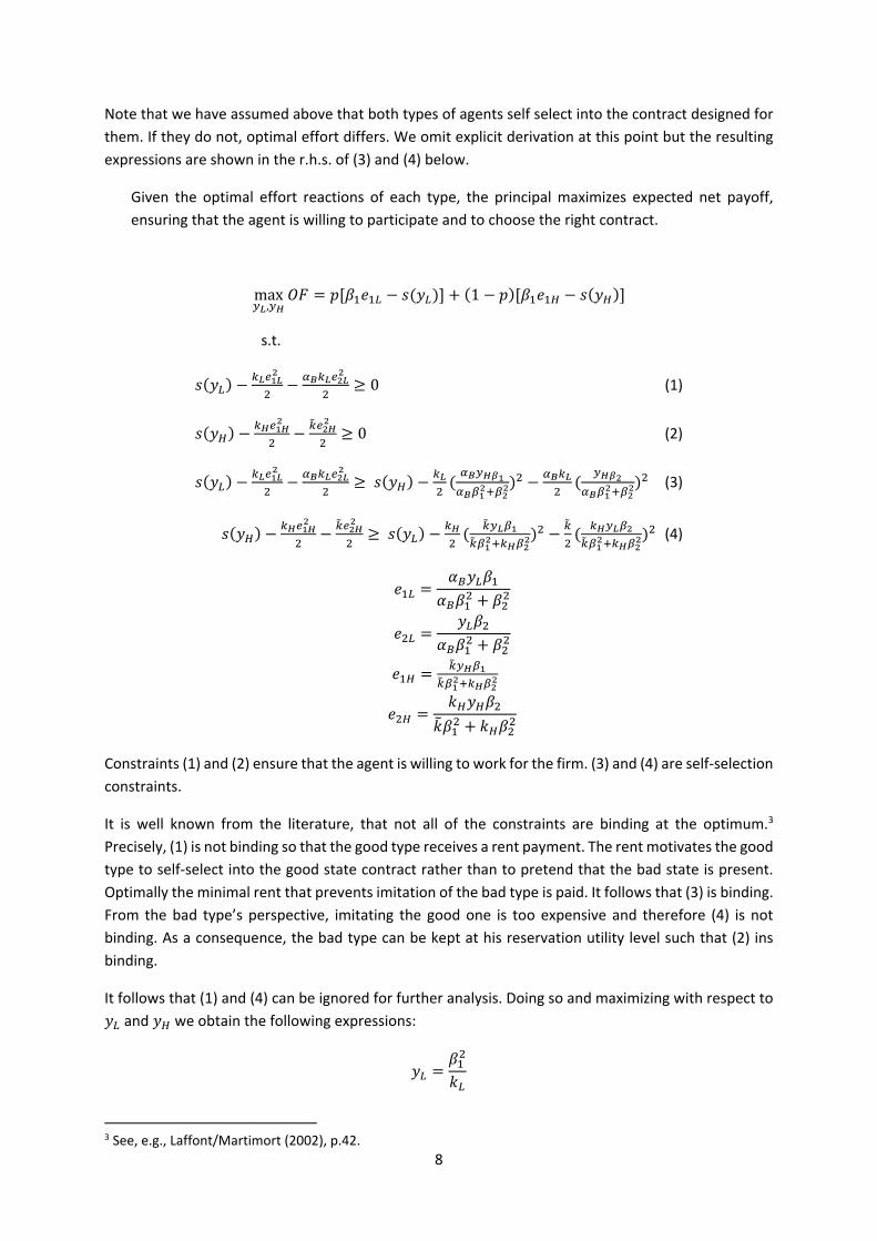
Note that we have assumed above that both types of agents self select into the contract designed for
them. If they do not, optimal effort differs. We omit explicit derivation at this point but the resulting
expressions are shown in the r.h.s. of (3) and (4) below.
Given the optimal effort reactions of each type, the principal maximizes expected net payoff,
ensuring that the agent is willing to participate and to choose the right contract.
max,
1
s.t.
0 (1)
0 (2)
(3)
(4)
Constraints (1) and (2) ensure that the agent is willing to work for the firm. (3) and (4) are self‐selection
constraints.
It is well known from the literature, that not all of the constraints are binding at the optimum.3
Precisely, (1) is not binding so that the good type receives a rent payment. The rent motivates the good
type to self‐select into the good state contract rather than to pretend that the bad state is present.
Optimally the minimal rent that prevents imitation of the bad type is paid. It follows that (3) is binding.
From the bad type’s perspective, imitating the good one is too expensive and therefore (4) is not
binding. As a consequence, the bad type can be kept at his reservation utility level such that (2) ins
binding.
It follows that (1) and (4) can be ignored for further analysis. Doing so and maximizing with respect to
and we obtain the following expressions:
3 See, e.g., Laffont/Martimort (2002), p.42.
9
with ∆
Note that only , but not , is a function of , , and .
Inserting once again into the optimal effort expressions and the objective function of the principal we
obtain the results stated in lemma 2.
Lemma 2: The optimal solution to the joint moral hazard and adverse selection problem is
characterized by
∗
∗
∗
∗
∆ ∆
∆ ∆.
6. SimplifiedSettingsA‐C
In order to be able to interpret the above results properly we will proceed looking at several simplified
settings bevor we tackle the full model.
An overview of the results is presented in the table below and each setting is discussed in detail in
sections 6.1‐6.3.

10
∆∗
∆1
21
∆∆
1
∆∗
∆1
21
∆∆
1
∆∗
∆1
2∆1
∆1
∗
2
∆1
2
2
1
∆2
1∆
2
1
∆2
1∆
∗
∗
∗
∗
∆1
∗
∗
∗
∆1
∗
∗
∆1
∗
∗0
∗∗
0
∗
∗
∗
11
∆
∗
∗
∗
11
∆
∗
∗
∗
∗1
∆1
∗
∗
∗
11
∆
∗
∗
∗
11
∆
Type of
agen
cy
problem
MH
MHAS
MH
MHAS
MH
MHAS
Setting n
A.
0
B.
1
C.
==
1
Table 1: Results from simplified settings.

11
6.1 SettingA
As a first step, and to provide the most basic insights into the trade‐off between moral hazard and the
joint setting, we assume 0. This implies that only the productive effort enters the performance
measure. Performing a window dressing activity therefore is of no value for the agent. Accordingly,
0 is optimal and introducing an accounting system that renders window dressing activities more
costly is of no effect and useless for the principal.
If a pure moral hazard problem is present, the first best solution can be implemented. All the risk,
which is entirely related to the unknown actual disutility of effort, is transferred to the agent. As the
agent is risk neutral, this is without costs. The result thus resembles a “selling the shop to the agent”
type of solution. Choosing ∗ appropriately allows the principal to induce the first best effort at first
best cost.
Given an adverse selection problem is present on top, first best can no longer be achieved. Rather,
agency costs occur due to incentives of the good type to imitate the bad type. Incentives of the bad
type are downward distorted in equilibrium in order to reduce rent payments to the good type at the
cost of sacrificing effort incentives for the bad type. At the same time, incentives for the good type
remain undistorted, a result known from the literature as “no distortion at the top”. It is reflected in
our model by ∗ ∗ along with ∗ ∗ .
Achieving first best in the moral hazard setting while achieving second best in the joint setting,
however, by no means implies that pure moral hazard is generally preferred to joint moral hazard and
adverse selection. This shows if we compare objective function values in both settings and leads to
proposition 1.
Proposition 1: The principal prefers to hire an informed agent, if ∆ is greater than .
Otherwise, he prefers to hire an uninformed manager.
Inspecting the difference in setting A,
∆
∆ ∆∆
we observe that it is composed of a difference ∆ multiplied by a positive factor.4 It follows that
the difference in objective function values is positive, whenever ∆2 is positive. is a factor that puts some weight on the disutility of effort the agent suffers
from. If the weights are sufficiently different depending on the working environment, the adverse
selection/moral hazard setting is preferred to the pure moral hazard setting.
In a pure moral hazard setting the manager is uninformed. This keeps him from exploiting private
knowledge to the detriment of the principal. It also keeps him, however, from fine‐tuning his effort to
the situation at hand. If the states of nature, tantamount to the working environments, are not too
distinct, costs related to the lack of fine‐tuning are lower than costs from exploiting private knowledge.
Hiring an uninformed manager is preferred. If, in contrast, the states of nature become more distinct,
private knowledge and fine‐tuning of effort becomes more valuable and related benefits beat the cost
resulting from asymmetric information. It becomes preferable for the principal to hire an informed
4 We assume at this point that ∆ 0 and 1, such that two distinct types exist at all.
12
manager, even though this involves a rent payment if working conditions are good along with
downward distorted incentives for the agent in the bad environment.
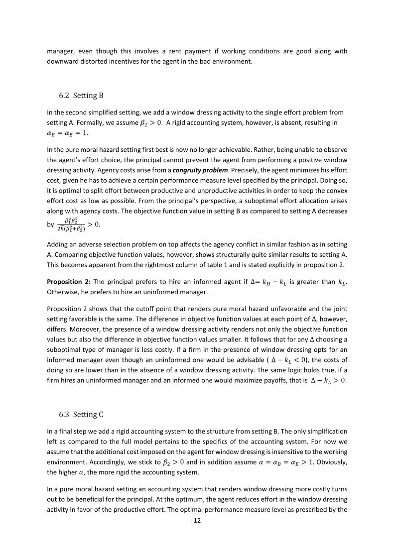
6.2 SettingB
In the second simplified setting, we add a window dressing activity to the single effort problem from
setting A. Formally, we assume 0. A rigid accounting system, however, is absent, resulting in
1.
In the pure moral hazard setting first best is now no longer achievable. Rather, being unable to observe
the agent’s effort choice, the principal cannot prevent the agent from performing a positive window
dressing activity. Agency costs arise from a congruity problem. Precisely, the agent minimizes his effort
cost, given he has to achieve a certain performance measure level specified by the principal. Doing so,
it is optimal to split effort between productive and unproductive activities in order to keep the convex
effort cost as low as possible. From the principal’s perspective, a suboptimal effort allocation arises
along with agency costs. The objective function value in setting B as compared to setting A decreases
by 0.
Adding an adverse selection problem on top affects the agency conflict in similar fashion as in setting
A. Comparing objective function values, however, shows structurally quite similar results to setting A.
This becomes apparent from the rightmost column of table 1 and is stated explicitly in proposition 2.
Proposition 2: The principal prefers to hire an informed agent if ∆ is greater than .
Otherwise, he prefers to hire an uninformed manager.
Proposition 2 shows that the cutoff point that renders pure moral hazard unfavorable and the joint
setting favorable is the same. The difference in objective function values at each point of ∆, however, differs. Moreover, the presence of a window dressing activity renders not only the objective function
values but also the difference in objective function values smaller. It follows that for any ∆ choosing a suboptimal type of manager is less costly. If a firm in the presence of window dressing opts for an
informed manager even though an uninformed one would be advisable ( ∆ 0), the costs of doing so are lower than in the absence of a window dressing activity. The same logic holds true, if a
firm hires an uninformed manager and an informed one would maximize payoffs, that is ∆ 0.
6.3 SettingC
In a final step we add a rigid accounting system to the structure from setting B. The only simplification
left as compared to the full model pertains to the specifics of the accounting system. For now we
assume that the additional cost imposed on the agent for window dressing is insensitive to the working
environment. Accordingly, we stick to 0 and in addition assume 1. Obviously, the higher , the more rigid the accounting system.
In a pure moral hazard setting an accounting system that renders window dressing more costly turns
out to be beneficial for the principal. At the optimum, the agent reduces effort in the window dressing
activity in favor of the productive effort. The optimal performance measure level as prescribed by the

13
principal, ∗, remains unaffected. A stricter accounting system thus helps to mitigate the congruity
problem and increases the principal’s objective function. The effect is stronger the higher .
The identified effects remain if an adverse selection problem is added. A stricter accounting system
increases productive effort, decreases window dressing and increases the principal’s objective function
value for any given .The optimal performance measure values are still independent of , too.
Proposition 3: The principal again prefers to hire an informed agent, if ∆ is greater than .
Otherwise, he prefers to hire an uninformed manager.
Proposition 3 shows that the solutions are structurally similar to both the previous settings. The cutoff
point is once more the same. The difference in objective function values at each point of ∆ again differs. As compared to the setting with 1 differences are larger for each ∆ and thus it becomes more
costly again if the wrong type of manager is chosen.
In all scenarios, however, we find that it is optimal to hire an uninformed manager if ∆ is sufficiently low and an informed manager if it becomes sufficiently high. There is only a single point of indifference
beyond the one when ∆→ 0. When ∆ increases, objective function values obtained from hiring either
type of manager are decreasing. To the left hand side of the point of indifference, the objective
function value from the joint setting decreases at a higher rate. On the right hand side of the point of
indifference, the objective function value obtained in the pure moral hazard setting decreases at a
higher rate.
To demonstrate the general pattern we use a numerical example and plot the optimal objective
function values varying ∆.
Numerical example 1: 1,5; 2; 1,5; 0.6; 1,2
Figure 1: Change in objective function values in , example 1.
.
0.5 1.0 1.5 2.0 2.5 3.0
0.6
0.7
0.8
0.9
1.0
1.1
1.2

14
7. Backtothefullmodel
Now we not only allow for a window dressing activity that is restricted by an accounting system but
also for the basic cost factor to differ from the extra one, .
Inspecting the differences in objective function values again, we find that several characteristics from
the simplified settings above continue to hold in this setting. We formalize them again in proposition
4 i), ii) and iv). Proposition 4 iii), however, identifies a structural difference that will be discussed
below.
Proposition4:
i) Both objective function values coincide in the lower limit, that is lim∆→
lim∆→
.
ii) If ∆ approaches infinity always holds.
iii) Arbitrarily close to zero the objective function value under pure moral hazard decreases
at a higher rate or increases at a lower rate than the objective function value in the joint
setting, that is ∆
0∆
0 always holds.
iv) There is a single point of indifference where .
Given i) to iv), it follows that there is always a lower range of ∆ in which the objective function value is higher in the pure moral hazard setting and an upper range in which the joint setting results in higher
objective function values. To that extent the results are structurally similar to the ones derived in the
simplified settings A‐C. A difference worth looking into, however, is that objective function values are
not necessarily continuously decreasing in ∆ anymore as stated in iii). Rather, there might be an
increase in objective function values for sufficiently low ∆, and a decrease after a maximum is reached.
Possible (additional) shapes are depicted for two numerical examples.
In the first example objective function values in both settings are increasing in ∆ if ∆ is small. We used
the following parameter values for numerical example 2: 1,5, 15; 2; 1,5;0.1; 1,2.
Figure 2: Change in objective function values in , example 2.
0.5 1.0 1.5 2.0 2.5 3.0
0.6
0.8
1.0
1.2

15
In the second example increases for ∆ sufficiently small, reaches a maximum and then
decreases. In the joint setting, in contrast, is strictly decreasing over the feasible range.
Parameters used in numerical example 3 are : 1,5, 15; 2; 1,5; 0.6; 1,2.
Figure 3: Change in objective function values in , example 3.
The distinct shapes, that is the existence of an inner maximum of objective function values in some
settings, result from our model assumptions with respect to disutility of both types. Recall that we
assume the disutility of effort for the good type equals and it is ∆ ∆
for the bad type.
As argued above already, disutility of both types becomes identical if the types vanish, that is ∆→ 0. All our graphs start from that very point, ∆ 0. At this point the cost factor is of no effect and the
amount of window dressing depends on only. Once ∆ becomes positive, however, gets
relevant. If is sufficiently high ( note in example 2 and 3 we assume 15 along with 1.5), even a small increase in ∆ results in extraordinary costs of window dressing and in turn leads to a strong decrease of window dressing and a shift towards productive effort. This is what drives the
increase in the objective function value for a lower range of ∆. Once the difference in types increases further, however, costs of disutility still increase but the already small amount of window dressing
declines with limited cost effects. Rather, costs from a lack of fine‐tuning due to missing information
(MH) and costs from the threat of imitation (MHAS) become predominant again and after reaching a
maximum, objective function value starts to decrease.
Differences in the objective function shape in both settings as shown in figure 3, result from distinct
effects of ex ante probability for the good and the bad type, . In the pure moral hazard setting the
agent does not know his own type. Even if the probability for a good environment is relatively high,
0,6 in example 3, there is still a 0,4 probability to suffer extreme disutility from window dressing.
As a result, the agent refrains strongly from window dressing and the positive effect on the objective
function value as described above arises. In the joint setting, in contrast, with ex ante probability of
0.5 1.0 1.5 2.0 2.5 3.0
0.8
0.9
1.0
1.1
1.2
16
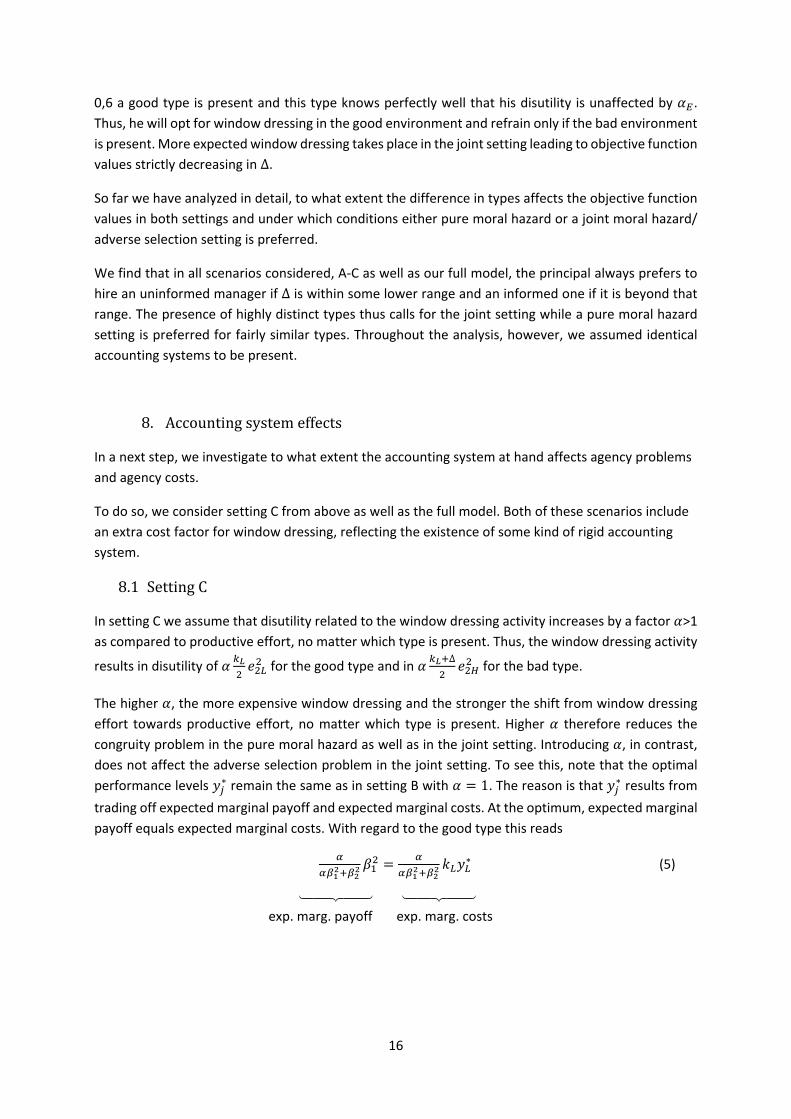
0,6 a good type is present and this type knows perfectly well that his disutility is unaffected by .
Thus, he will opt for window dressing in the good environment and refrain only if the bad environment
is present. More expected window dressing takes place in the joint setting leading to objective function
values strictly decreasing in ∆.
So far we have analyzed in detail, to what extent the difference in types affects the objective function
values in both settings and under which conditions either pure moral hazard or a joint moral hazard/
adverse selection setting is preferred.
We find that in all scenarios considered, A‐C as well as our full model, the principal always prefers to
hire an uninformed manager if ∆ is within some lower range and an informed one if it is beyond that
range. The presence of highly distinct types thus calls for the joint setting while a pure moral hazard
setting is preferred for fairly similar types. Throughout the analysis, however, we assumed identical
accounting systems to be present.
8. Accountingsystemeffects
In a next step, we investigate to what extent the accounting system at hand affects agency problems
and agency costs.
To do so, we consider setting C from above as well as the full model. Both of these scenarios include
an extra cost factor for window dressing, reflecting the existence of some kind of rigid accounting
system.
8.1 SettingC
In setting C we assume that disutility related to the window dressing activity increases by a factor >1
as compared to productive effort, no matter which type is present. Thus, the window dressing activity
results in disutility of for the good type and in ∆
for the bad type.
The higher , the more expensive window dressing and the stronger the shift from window dressing
effort towards productive effort, no matter which type is present. Higher therefore reduces the
congruity problem in the pure moral hazard as well as in the joint setting. Introducing , in contrast,
does not affect the adverse selection problem in the joint setting. To see this, note that the optimal
performance levels ∗ remain the same as in setting B with 1. The reason is that ∗ results from
trading off expected marginal payoff and expected marginal costs. At the optimum, expected marginal
payoff equals expected marginal costs. With regard to the good type this reads
∗ (5)
exp. marg. payoff exp. marg. costs
17
Likewise, for the bad type we get
1 ∗ 1 ∆ (6)
exp. marg. payoff exp. marg. costs
Note that for the good type marginal costs equals marginal disutility from efforts while for the bad
type an extra cost factor captures marginal costs from rent payments, that is ∗ ∆. More important,
however, we observe that always is part of a common multiplicative factor on both sides of the
equations. Thus, any increase of affects marg. payoff and marg. costs in identical fashion and leaves ∗ the same. It follows that the downward distortion of the bad type’s performance level remains the
same as in setting B and so are agency costs related to the adverse selection problem. It follows that
the objective function values in both settings increase in . Summing this up results in proposition 5.
Proposition 5:
In a pure moral hazard setting we find that
∗
0, ∗
0, ∗
0,and ∗
0
It is optimal to choose → ∞, or, alternatively, as large as possible.
In the joint setting we find
∗
0, ∗
0, ∗
0, ∗
0, ∗
0, ∗
0,and ∗
0.
It is optimal to choose → ∞, or, alternatively, as large as possible.
It follows directly from proposition 5 that in both settings, pure moral hazard and joint setting, any
accounting system that exhibits higher is preferred to one with lower .
8.2 Full model
Considering the full model that allows for , we find that results in the pure moral hazard
setting are structurally identical to those from setting C. Higher factors and shift effort from the
window dressing activity towards the productive activity in equilibrium. Increasing and reduces
the congruity problem and in turn increases the objective function value for the principal. This will be
stated formally in proposition 6 a) below.
In the joint setting, the effects of and on the congruity problem remain unchanged as compared
to setting C (and the pure moral hazard problem in this section) as well, as is shown in proposition 6 b)
below.

18
The effects on the adverse selection problem, in contrast, are fundamentally different. With respect
to the good type, ∗ is still independent of any increase in s. It is independent from changes in
as the good type by definition is unaffected by the extra cost. Recall his disutility has been defined
. Moreover, it is independent from as the expected marginal payoffs and costs
resemble those from (5) if we replace by . The common factor argument remains valid.
For the bad type, in contrast, this is no longer true. Different from (6) there is no longer a common
factor that affects marginal payoff and costs in similar fashion if . Rather, the bad type’s performance level becomes a function of both, and and equals
∗∆
.
Note that in the absence of any incentive to imitate, the performance level for the bad type chosen by
the principal would be . In settings A‐C a unique level of downward distortion of this
performance level has been identified as ∗∆ < . It follows that agency costs from adverse
selection have been present already in settings A‐C. The distortion factor, ∆, can be regarded as a
measure of the strengths of the adverse selection problem.
Now, in the full model, the downward distortion factor is . It can be larger or smaller than ∆. The
distortion is larger (smaller) in the full model if as >(<) ∆
if . It is
therefore not clear whether the adverse selection problem is more or less severe in the full model as
in the simplified ones. We can identify, however, a combination of and that minimizes . It holds
that ∆. This is presented in proposition 6 b) ii) below.
Proposition6:
a) In a pure moral hazard setting
∗
0, ∗
0,∗
0, ∗
0, ∗
0, ∗
0, and ∗
0,∗
0.
It is optimal to choose each of → ∞ with , , or, alternatively, as large as possible.
b) In the joint setting
i) the congruity problem is minimized for → ∞ with , .
ii) the downward distortion in ∗ , is minimized if distortion factor is minimal. This is
achieved for → 1 and → 1.
It follows from proposition 6 that it is not necessarily optimal any longer to choose and as large
as possible in the joint setting. Doing so reduces the congruity problem but may increase the adverse
selection problem. As shown in proposition 6b) ii), the distortion factor is minimized when is
chosen as small as possible and an inner solution is obtained for . To see the economic rationale of
19
this result, note that the adverse selection problem becomes stronger if the types become more
distinct. As the types in our model differ in their disutility, an increase in increases the badtype’sdisutility from effort relative to the good type’s. Both types drift apart and in turn the adverse selection
problem becomes harder.
The optimal results from trading off costs from the congruity problem and costs from the adverse
selection problem. We find that the optimal critically depends on the probability for a good or bad
environment to be present. If the probability for a good type is smaller than for a bad one, that is
0.5, the adverse selection problem is sufficiently small to be dominated by the congruity problem. Any
increase in increases the objective function value for any given . If, in contrast, the good type is
more likely, the adverse selection problem becomes more important. The principal’s objective function
is strictly decreasing in or it decreases in lower ranges of , reaches a minimum, and then
increases. Both is shown in proposition 7 and also illustrated in figure 4 and figure 5 below.
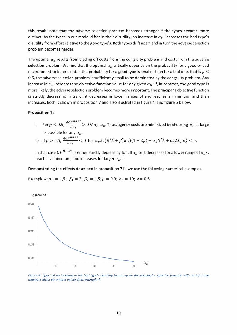
Proposition 7:
i) For 0.5, 0∀ , . Thus, agency costs are minimized by choosing as large
as possible for any .
ii) If 0.5, 0 for 1 2 ∆ 0.
In that case is either strictly decreasing for all or it decreases for a lower range of ,
reaches a minimum, and increases for larger .
Demonstrating the effects described in proposition 7 ii) we use the following numerical examples.
Example 4: 1,5; 2; 1,5; 0.9; 10;∆ 0,5.
Figure 4: Effect of an increase in the bad type’s disutility factor on the principal’s objective function with an informed manager given parameter values from example 4.
10 20 30 40 50
0.137
0.138
0.139
0.140
0.141

20
Example 5: 1,5; 2; 1,5; 0.9; 10;∆ 5.
Figure 5: Effect of an increase in the bad type’s disutility factor on the principal’s objective function with an informed manager given parameter values from example 5.
To summarize, we find that the choice of hiring an uninformed manager versus an informed manager
and the choice of an appropriate accounting system are interrelated. If an uninformed manager is
hired, it is always favorable to implement an accounting system that increases the manager’s disutility
from window dressing by any amount. The most favorable system is the one that increases costs as
much as possible. If an informed manager is hired, in contrast, it can be detrimental to replace an
accounting system that exposes the bad type to a low cost factor of disutility, , by one that exhibits
a higher cost factor. Two scenarios are possible. In the first one any accounting system that increases
is detrimental. In the second, it might be detrimental to increase by a small amount but
beneficial to increase it by a sufficiently large amount.
9. Conclusion
In this paper we analyze, under which conditions a principal benefits from hiring an outside manager
as opposed to an inside manager. We find that the principal prefers to hire an outside manager if the
manager’s types, reflected in the disutility related to effort, are not too distinct.
Intuitively the principal trades off costs and benefits from private managerial pre‐contract information.
An outside manager has no such information. He cannot fine‐tune his effort choice nor can he exploit
his private knowledge to extract rents from the principal. An insider, in contrast, has both these
options. If the types are quite similar, costs related to suboptimal effort choice are lower than costs
from rent extraction. It follows that the principal optimally hires an outsider. For very distinct types,
costs related to a lack of fine tuning in effort choice increase and exceed costs from rent extraction. In
such a setting the principal is better off, hiring an insider. Given an identical accounting system in place,
0 10 20 30 40 50
0.13324
0.13325
0.13326
0.13327
0.13328

21
no matter which hiring choice is made by the principal, we identify some critical type difference at
which the principal is indifferent with respect to his hiring choice in all our settings.
Analyzing the effect of a more or less rigid accounting system in both, a moral hazard and a joint moral
hazard and adverse selection setting separately, we find that a more restrictive system is always
preferred with moral hazard. In the joint setting this is no longer the case. Rather, the principal’s payoff
may decrease if the accounting system becomes more rigid. This is the case when the system renders
the types of managers more distinct and thus amplifies the adverse selection problem.
While we have interpreted the distinct information endowment of managers as due to “inside” versus
“outside” applicants to the firm, this is certainly not the only possible story to be told. Alternatively,
we could assume that information asymmetry arises if one applicant is an insider to the industry but
not the firm, while another one is an outsider to the industry. Another interpretation could be that
private information results from work experience in management positions in general while a rookie
manager does not possess this type of information.
10. Literature
Arya, A., Glover, J., Sunder, S. (1998) Earnings Management and the Revelation Principle, Review of
Accounting Studies, 3, (1‐2), 7‐34.
Beyer, A., Guttman, I., Marinovic, I. (2014) Optimal Contracts with Performance Manipulation,
Journal of Accounting Research, 52 (4), 817‐847.
Demski, J. (1998) Performance Measure Manipulation, Contemporary Accounting Review 15, 261‐
285.
Dye, R. (1988) Earnings Management in an Overlapping Generations Model, Journal of Accounting
Research 26, 195‐235.
Ewert, R., Wagenhofer, A. (2005) Economic Effects of Tightening Accounting Standards to Restrict
Earnings Management, The Accounting Review 80 (4), 1101‐1124.
Feltham, G., Xie, J. (1994) Performance Measure Congruity and Diversity in Multi‐Task
Principal/Agent Relations, The Accounting Review 69 (3), 429‐453.
Goldmann, E., Slezak, S. (2006) An Equilibrium Model of Incentive Contracts in the Presence of
Information Manipulation, Journal of Financial Economics, 603‐626.
Grossmann, S. Hart, O. (1983) An Analysis of the Principal‐Agent Problem, Econometrica 51, 7‐45.
Holmström, B. (1979) Moral Hazard and Observability, The Bell Journal of Economics 10, 74‐91.
Holmström, B., Milgrom, P. (1991) Multitask Principal‐Agent Analyses: Incentive Contracts, Asset
Ownership, and Job Design, Journal of Law, Economics and Organization 7, 24‐52.
Laffont, J., Martimort, D. (2002) The Theory of Incentives, Princeton University Press.
22
Laffont, J., Tirole, J. (1993) A Theory of Incentives in Procurement and Regulation, Massachusetts
Institute of Technology.
Marinovic, I., Povel, P. (2017) Competition for Talent under Performance Manipulation, Journal of
Accounting and Economics 64 (1), 1‐14.
Melumad, N., Reichelstein, S. (1989) Value of Communication in Agencies, Journal of Economic
Theory 47, 334‐368.
Murphy, K. (2013) Executive Compensation: Where we are, and how we got there, in:
Constantinides, C., Harris, M., Stulz, R., eds, Handbook of the Economics of Finance, Vol. 2, Elsevier
Science North Holland, 211‐356.
Rajan, M., Saouma, R. (2006) Optimal Information Asymmetry, The Accounting Review, 81 (3), 677‐
712.
Sappington, D. (1984) Incentive Contracting with Asymmetric and Imperfect Precontractual
Knowledge, Journal of Economic Theory, 52‐70.
Appendix
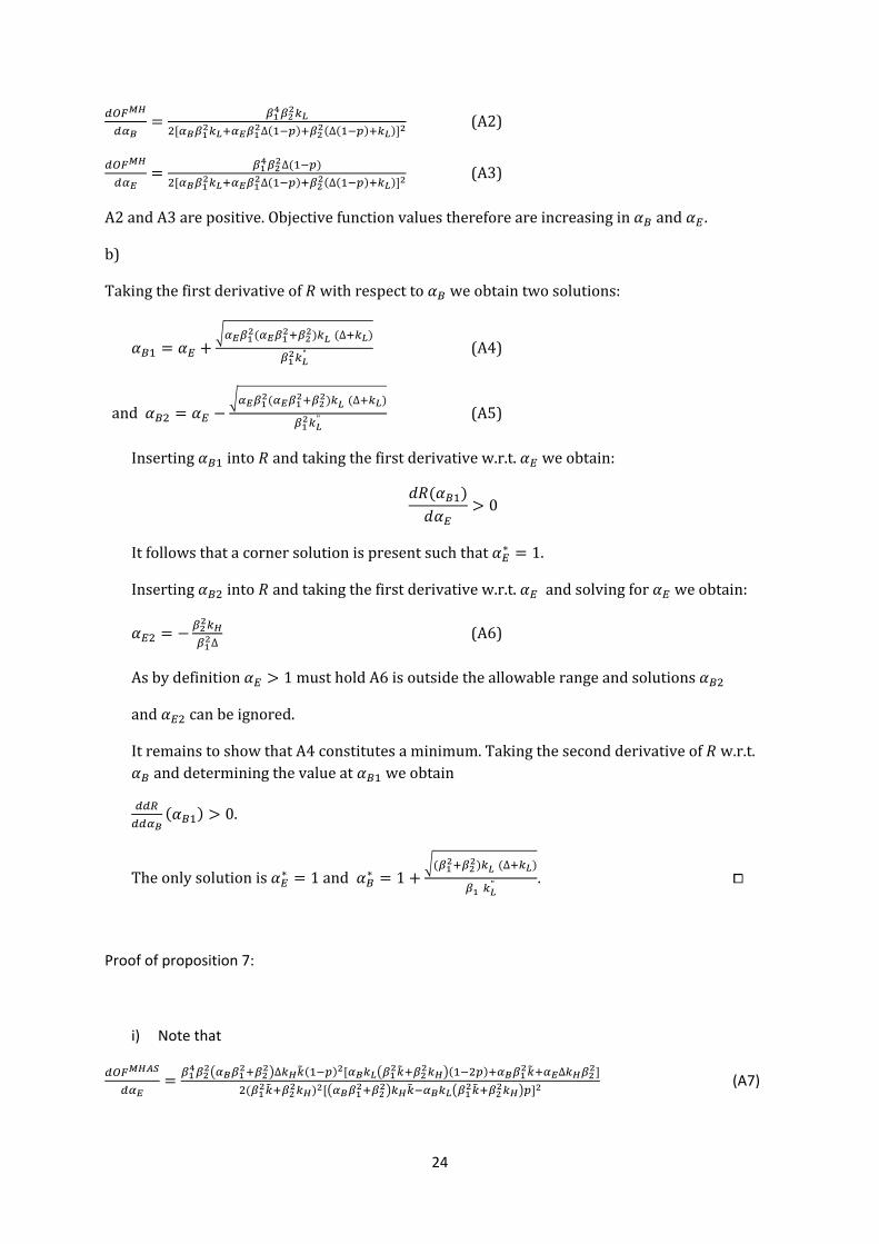
Proof of proposition 4:
i) lim∆→
lim∆→
.
ii) lim∆→
0, lim∆→
iii) Firstorderconditionforamaximumof equals:
∆
0
Solvingfor∆weobtain:
∆1 1
10
∆1 1
10
Itfollowsthataninnerextremevalueexistsifandonlyif∆ 0.Otherwise,noinnerextremevalueexists.Therecannotbemorethanoneinnerextremevalueas∆ isnotintheallowablerange.

23
Usingthesameprocedurewithregardto weobtainsimilarresults:
Solvingfor∆weobtain:∆ 0and∆ 0.Again,oneinnerextremevalueexistsifandonlyif∆ 0.Otherwisenoinnerextremevalueexists.
Ifaninnerextremevalueexists,ithastobeamaximum.Toseethis,recallfromi)andii)that
lim∆→
> lim∆→
0.Inadditionlim∆→
lim∆→
.Bothobjectivefunctionvaluesaredecreasingoverall.Iftheextreme
valuewasaminimum,someobjectivefunctionvaluesbelow lim∆→
0andlim∆→
wouldhavetoexist.This,however,isnotthecaseas 0and
forall∆.
Itfollowsthattheobjectivefunctionvaluesinbothsettingscaneitherbedecreasingin∆ortheycanbeincreasingforsmall∆,reachamaximum,anddecreasebeyond.
Define∆
0∆
0 .
0 (A1)
FromtheabovefindingsandA1itfollowsthatarbitrarily close to zero the objective function value under pure moral hazard decreases at a higher rate or increases at a lower rate than the objective
function value in the joint setting.
iv) Becauseofiii)itcaneitherbethecasethat
∆0 0and
∆0 0,thatisbothobjectivefunctionsaredecreasingin∆andno
innermaximumexistsineithersetting,or
∆0 0and
∆0 0,thatisbothobjectivefunctionsareincreasingfor
sufficientlysmall∆anddecreasebeyondamaximuminbothsettings,or
∆0 0and
∆0 0,thatisinthemoralhazardsettingtheobjectivefunction
valueincreasesandreachesamaximumbeforedecreasingin∆.Inthejointsetting,theobjectivefunctionvaluedecreasesforall∆.
Nomatterwhichoftheabovescenariosispresent,giventheconditionsidentifiedini),ii)andiii)therecanbeonlyasinglepointofindifference.Forvaluessmaller(greater)thanacritical∆,
. ⧠
Proofofproposition6:
a)
24
∆ ∆ (A2)
∆
∆ ∆ (A3)
A2andA3arepositive.Objectivefunctionvaluesthereforeareincreasingin and .
b)
Takingthefirstderivativeof withrespectto weobtaintwosolutions:
∆
" (A4)
and∆
" (A5)
Inserting into andtakingthefirstderivativew.r.t. weobtain:
0
Itfollowsthatacornersolutionispresentsuchthat ∗ 1.
Inserting into andtakingthefirstderivativew.r.t. andsolvingfor weobtain:
∆ (A6)
Asbydefinition 1mustholdA6isoutsidetheallowablerangeandsolutions
and canbeignored.
ItremainstoshowthatA4constitutesaminimum.Takingthesecondderivativeof w.r.t.anddeterminingthevalueat weobtain
0.
Theonlysolutionis ∗ 1and ∗ 1∆
" . ⧠
Proof of proposition 7:
i) Note that
∆ ∆ (A7)

25
The denominator of A7 is positive. The numerator is always positive if 1 2 0, that is 0.5.
In that case 0 ∀ , .
ii) With 0.5 the numerator of A7 can be positive or negative. Solving the optimality
condition 0 for we get a single solution that might be in the allowable range of
1.
∗ 2 1 2 1 ∆
∆ ∆ 1 2
Taking the second derivative of and evaluate at ∗ we obtain
∗ ∆ 1 ∆ 1 20
It follows that any extreme value that might exist constitutes a minimum.
Note that 0 if 1 2 ∆ 0.
If this condition holds for all 1, is strictly decreasing. If ∗ is in the allowable
range, is decreasing for low , reaches a minimum at ∗ and increases for larger .
⧠