Hinze, R., & Wu, N. (2016). Unifying Structured Recursion ...
48
Hinze, R., & Wu, N. (2016). Unifying Structured Recursion Schemes. Journal of Functional Programming, 26, [e1]. DOI: 10.1017/S0956796815000258 Peer reviewed version Link to published version (if available): 10.1017/S0956796815000258 Link to publication record in Explore Bristol Research PDF-document University of Bristol - Explore Bristol Research General rights This document is made available in accordance with publisher policies. Please cite only the published version using the reference above. Full terms of use are available: http://www.bristol.ac.uk/pure/about/ebr-terms.html brought to you by CORE View metadata, citation and similar papers at core.ac.uk provided by Explore Bristol Research
Transcript of Hinze, R., & Wu, N. (2016). Unifying Structured Recursion ...
Hinze, R., & Wu, N. (2016). Unifying Structured Recursion Schemes.Journal of Functional Programming, 26, [e1]. DOI:10.1017/S0956796815000258
Peer reviewed version
Link to published version (if available):10.1017/S0956796815000258
Link to publication record in Explore Bristol ResearchPDF-document
University of Bristol - Explore Bristol ResearchGeneral rights
This document is made available in accordance with publisher policies. Please cite only the publishedversion using the reference above. Full terms of use are available:http://www.bristol.ac.uk/pure/about/ebr-terms.html
brought to you by COREView metadata, citation and similar papers at core.ac.uk
provided by Explore Bristol Research

ZU064-05-FPR URS 15 September 2015 9:20
Under consideration for publication in J. Functional Programming 1
Unifying Structured Recursion SchemesAn Extended Study
RALF HINZEDepartment of Computer Science, University of Oxford
NICOLAS WUDepartment of Computer Science, University of Bristol
(e-mail: [email protected], [email protected])
Abstract
Folds and unfolds have been understood as fundamental building blocks for total programming, andhave been extended to form an entire zoo of specialised structured recursion schemes. A great numberof these schemes were unified by the introduction of adjoint folds, but more exotic beasts such asrecursion schemes from comonads proved to be elusive. In this paper, we show how the two canonicalderivations of adjunctions from (co)monads yield recursion schemes of significant computationalimportance: monadic catamorphisms come from the Kleisli construction, and more astonishingly, theelusive recursion schemes from comonads come from the Eilenberg-Moore construction. Thus wedemonstrate that adjoint folds are more unifying than previously believed.
1 Introduction
Functional programmers have long realised that the full expressive power of recursion isuntamable, and so intensive research has been carried out into the identification of an entirezoo of structured recursion schemes that are well-behaved and more amenable to programcomprehension and analysis (Meijer et al., 1991).
The foundational structured recursion operators are catamorphisms or folds and anamor-phisms or unfolds (Hagino, 1987; Malcolm, 1990b): they make termination or progressmanifest, and enjoy many useful calculational properties which would otherwise have to beestablished afresh for each new application.
However, catamorphisms and anamorphisms are relatively restricted. There are manyother structured patterns of recursion, equally well behaved and worth capturing, that donot quite fit the scheme. Variations on catamorphisms that have been proposed in the pastinclude folds with parameters and accumulating folds (Pardo, 2002), which may dependon constant or varying additional arguments; mutumorphisms (Fokkinga, 1990), which arepairs of mutually recursive functions; zygomorphisms (Malcolm, 1990a), which consist of amain recursive function and an auxiliary one on which it depends; paramorphisms (Meertens,1992), in which the body of structural recursion has access to immediate subterms as wellas to their images under the recursion; histomorphisms (Uustalu & Vene, 1999b), in whichthe body has access to the recursive images of all subterms, not just the immediate ones;

ZU064-05-FPR URS 15 September 2015 9:20
2 R. Hinze and N. Wu
and so-called generalised folds (Bird & Paterson, 1999), which use polymorphic recursionto handle nested datatypes.
As variations on anamorphisms, there are apomorphisms (Vene & Uustalu, 1998), whichmay generate subterms monolithically rather than step by step; futumorphisms (Uustalu &Vene, 1999b), which may generate multiple levels of a subterm in a single step, rather thanjust one; and many other anonymous schemes that dualize better known inductive patternsof recursion.
The many divergent generalisations of catamorphisms can be bewildering to the unini-tiated, and there have been attempts to unify them. One approach is the identification ofrecursion schemes from comonads (Uustalu et al., 2001) which we call ‘rsfcs’ for short.Comonads capture the general idea of ‘evaluation in context’ (Uustalu & Vene, 2008),and rsfcs make contextual information available to the body of the recursion. This patternsubsumes zygomorphisms and histomorphisms.
A more recent attempt (Hinze, 2013) uses adjunctions as the common thread. Adjointfolds arise by inserting a left adjoint functor into the recursive characterisation, therebyadapting the form of the recursion; they subsume accumulating folds, mutumorphisms(and hence zygomorphisms), and generalised folds. Dually, adjoint unfolds involve a rightadjoint, and capture the production of a data structure in context; they subsume all the abovevariations on anamorphisms.
Given that adjoint folds and rsfcs cover some of the same examples, it seems reasonableto suspect a deeper relationship between them. That suspicion is strengthened by theobservation that every adjunction induces a comonad, and every comonad can be factoredinto adjoint functors. And indeed, the suspicion turns out to be well founded. In this paper,we show that rsfcs are subsumed by adjoint folds. Moreover, although the converse does nothold, we identify those adjoint folds that correspond to rsfcs.
This article is an extended and revised version of (Hinze et al., 2013), which in turn drawson material from (Hinze, 2013), although the technical presentation is quite different, makingessential use of liftings, distributive laws, and conjugates. Our technical contributions are asfollows, where the new material in this extended study is indicated by an open bullet point:
• We provide a fresh account of adjoint folds, making essential use of liftings andconjugates. Very briefly, adjoint folds are parametrised by an adjunction L a R and adistributive law σ : L◦D→̇C◦L that connects a data structure to a control structure.◦ We show that monadic catamorphisms (Fokkinga, 1994) are an instance of adjoint
folds using the Kleisli adjunction.• We show that rsfcs (Uustalu et al., 2001) are an instance of adjoint folds using the
(co)Eilenberg-Moore adjunction.• We state precisely the relationship to the (type) fusion rule of categorical fixed-
point calculus (Backhouse et al., 1995). In essence, type fusion allows us to fuse anapplication of a left adjoint with an initial algebra to form another initial algebra,L (µC)∼= µD, under the stronger assumption that σ is an isomorphism.
• We prove that adjoint folds can be framed as rsfcs, if σ is a distributive isomorphism.◦ We explore the calculational properties of adjoint folds, and show how the well-
established properties of other structured recursion schemes are instances of this moregeneral theory.

ZU064-05-FPR URS 15 September 2015 9:20
Unifying Structured Recursion Schemes 3
◦ We demonstrate the dual notion of adjoint unfolds, where a distributive law τ : D◦R→̇R◦Cconnects a decision structure to a codata structure.
We give three different definitions of adjoint folds: one in terms of Mendler-style folds,and one in terms of conjugates which leads to a canonical definition. The conjugate-based definition makes the proofs of uniqueness of schemes easier, where we dissect mostof the proofs into two parts: first, we establish a bijection between certain arrows andhomomorphisms; second, we instantiate the bijections to initial or free algebras.
The unified approach to recursion schemes is based on adjoint folds, folds and unfolds, sono new theory is needed. The message of this paper is that the existing theory is more generalthan we anticipated. The unification is more than merely an intellectual curiosity: it promisesconcrete returns, too—for example, through general techniques for combining differentrecursion schemes (most functions actually use a combination of recursion schemes).In addition, the unification also brings together the different calculational properties ofrecursion schemes under one umbrella, thus vastly reducing the number of laws requiredfor calculation.
The paper is organised as follows: Section 2 presents a smörgåsbord of Haskell examples,which are picked up later; Section 3 summarises some of the theoretical background;Section 4 discusses mutumorphisms as a basic example of our unifying theory of adjointfolds, which is set out in Section 5; Section 6 relates the discussion to zygomorphisms.Section 7 shows that all rsfcs are adjoint folds, and Section 8 identifies those adjointfolds that are rsfcs; we explore the Kleisli adjunction and its relationship to monadiccatamorphisms in Section 9; Section 10 discusses the calculational properties of adjointfolds; Section 11 shows the construction of adjoint unfolds; and finally, Section 12 discussesrelated work, and Section 13 concludes and points out directions for future work.
2 A Zoo of Morphisms
In this section we exhibit a number of specimens from the zoo of morphisms, which willserve to illustrate the theory that follows. We use Haskell as a widely appreciated linguafranca for codifying our categorical constructions as programs. Although Haskell conflatesinductive and coinductive types, our categorical development will be careful to distinguishbetween the two.
Catamorphism The most basic recursion scheme is the catamorphism, known morecolloquially as the fold of a data structure. A catamorphism decomposes an inductivelydefined structure, replacing each of the constructors with a provided function. An exampleof this pattern is to compute the depth of a binary tree.
data Tree = Empty | Node Tree N Tree
depth :: Tree→ Ndepth (Empty) = 0depth (Node l a r) = 1+(depth l ‘max‘ depth r)

ZU064-05-FPR URS 15 September 2015 9:20
4 R. Hinze and N. Wu
Folds with parameters Folds with constant parameters take an additional argument, onwhich results may depend. List concatenation is a canonical example:
cat :: ([a], [a ])→ [a]cat ([ ], ys) = yscat (x : xs,ys) = x : cat (xs,ys) .
Here, the second component of the input pair is the parameter; cat is not a fold because thepair argument is not of an inductive type.
In folds with accumulating parameters, the additional argument may vary in recursivecalls. Haskell’s foldl is an example. More interesting examples are provided by downwardsaccumulations on trees (Gibbons, 2000); for example, replacing every element with a labelof its depth (if the accumulator is initialised to 0):
depths :: (Tree,N)→ Treedepths (Empty, n) = Emptydepths (Node l a r,n) = Node (depths (l,n+1)) n (depths (r,n+1)) .
This is a rather simple example; in general, the accumulating parameter will vary in differentways in different branches.
Paramorphism The paramorphism models primitive recursion: the body has access notonly to the results of recursive calls, but also to the substructures on which these calls aremade. An example of a paramorphism is counting the words in a string:
wc :: [Char]→ Intwc [ ] = 0wc (c : cs)| ¬ (isSpace c) ∧ (null cs ∨ isSpace (head cs)) = wc cs+1| otherwise = wc cs .
Note that in the clause for non-empty lists, the result depends not only on a recursive callwc cs on the substructure, but also on the substructure cs itself.
Zygomorphism A variation is the zygomorphism, where the recursion is aided by anauxiliary function that is defined independently.
perfect :: Tree→ Bperfect Empty = Trueperfect (Node l a r) = perfect l ∧ perfect r ∧ (depth l depth r) .
The function perfect is not a simple fold, since it relies on an auxiliary traversal of the treestructure using depth.
Mutumorphism A mutumorphism generalises the idea of a zygomorphism, allowing therecursive functions to rely mutually on one another. For example, consider the odd and evenfunctions:
odd :: N→ B even :: N→ Bodd 0 = False even 0 = Trueodd (n+1) = even n even (n+1) = odd n .

ZU064-05-FPR URS 15 September 2015 9:20
Unifying Structured Recursion Schemes 5
Here, the functions work as a pair in tandem as they recurse through the structure of naturalnumbers.
Nested datatypes Functions over nested datatypes such as perfect trees or random-accesslists involve polymorphic recursion. For example, consider summing a perfect tree ofnumbers:
data Perfect a = Zero a | Succ (Perfect (a,a))
instance Functor Perfect wherefmap f (Zero a) = Zero (f a)fmap f (Succ p) = Succ (fmap (λ (x,y)→ (f x, f y)) p)
total :: Perfect N→ Ntotal (Zero n) = ntotal (Succ p) = total (fmap (λ (a,b)→ a+b) p) .
This is not a straightforward fold, because the recursive call of total is not applied directlyto a subterm—indeed, it cannot be so applied, because the subterm p of Succ p has typePerfect (N,N) rather than Perfect N.
Anamorphism The dual of a catamorphism is an anamorphism, or unfold. This corecursionscheme builds a structure from a single seed, one level at a time.
from :: Int→ [Int]from x = x : from (x+1)
This example builds an infinite stream of increasing integers starting from a given number.
Apomorphism An apomorphism can immediately return a subterm in its result, rather thanhaving to generate each part of the output structure through corecursion. An example is aninsertion into a sorted tree structure, where elements in left branches are less than or equalto the value in a node, and values in right branches are greater.
insert :: N→ Tree→ Treeinsert a Empty = Node Empty a Emptyinsert a (Node l b r) | a 6 b = Node (insert a l) b r
| otherwise = Node l b (insert a r)
This behaves like the unfolding of a tree in one branch, growing a new tree from the elementto be inserted and an existing tree, but in the other branch it immediately grafts a result.
Histomorphism Histomorphisms capture tabulation, as used in dynamic programming.For example, consider the unbounded knapsack problem: a knapsack of some fixed capacityis to be filled with items of varying weight and value. The goal is to maximise the total valueof the items contained in the knapsack. Suppose there is an infinite supply of items whoseweight and value can be drawn from the following list: [(12,4),(1,2),(2,2),(1,1),(4,10)].A knapsack with a capacity of 15 can be filled to a maximum value of 36 using three copieseach of the second and fifth items.

ZU064-05-FPR URS 15 September 2015 9:20
6 R. Hinze and N. Wu
The naive recursive solution takes exponential time (we suppose here that the maximumvalue of the empty list of candidate solutions is zero):
knapsack :: [(N,R)]→ N→ Rknapsack wvs c
= maximum0 [v+ knapsack wvs (c−w) | (w,v)← wvs,w 6 c] .
However, by tabulating the results for each capacity in 0 . .c, one can compute the answer inpseudo-polynomial time:
knapsack wvs c = table !! c wheretable = [ks i | i← [0 . .c ]]ks i = maximum0 [v+ table !! (i−w) | (w,v)← wvs,w 6 i ] .
Lazy evaluation works out the data dependencies automatically. However, each element ofthe table depends only on elements with lower indices, so even without lazy evaluation itsuffices to fill the table in index order.
Monadic catamorphism Monadic catamorphisms allow a monadic computation to bethreaded through the catamorphic traversal of a recursive structure. For example, thefunction accumulate takes a list of monadic actions and executes them each in turn, andreturns a list of their results in the monadic context.
accumulate :: Monad m⇒ [m a ]→ m [a ]accumulate [ ] = return [ ]
accumulate (mx : mxs) = mx>>=λx→ accumulate mxs>>=λxs→ return (x : xs)
When the input list is empty, we simply return the empty list in a monadic context. Otherwise,we run the monadic computation at the head of the list, and return the result of appending itto the accumulation of executed values in the tail.
Now, the general question is whether the recursion equations above have unique solutions?The answer is yes for all of them. However, up to now the proofs in the literature haveinvolved two seemingly incompatible techniques: most of the examples can be identified asadjoint folds; some of them (in particular knapsack) are subsumed by recursion schemesfrom comonads. Before we show how to unify the two approaches, we first need to introducea bit of theory.
3 Background
This paper assumes at least a basic knowledge of category theory, in that the reader shouldbe familiar with the notions of functors, natural transformations, as well as product andfunctor categories. In this section we fix the notation and establish categorical concepts thatwill be used in the remainder of the paper. For the most part this material is standard andcan safely be glossed over on an initial reading. An exception is perhaps the material onfunctor squares and conjugates, which will need particular attention.
ZU064-05-FPR URS 15 September 2015 9:20
Unifying Structured Recursion Schemes 7
3.1 Functor Squares and Distributive Laws
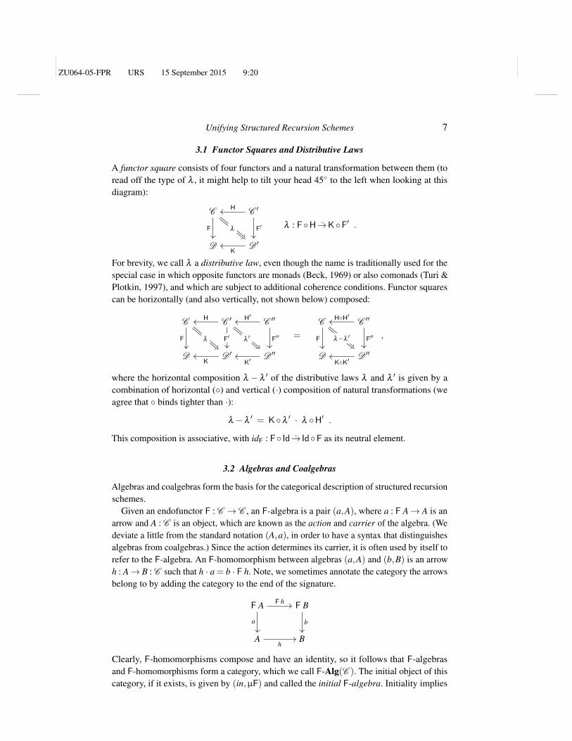
A functor square consists of four functors and a natural transformation between them (toread off the type of λ , it might help to tilt your head 45◦ to the left when looking at thisdiagram):
C C ′
D D ′
λF
H
F′
K
λ : F◦H→̇K◦F′ .
For brevity, we call λ a distributive law, even though the name is traditionally used for thespecial case in which opposite functors are monads (Beck, 1969) or also comonads (Turi &Plotkin, 1997), and which are subject to additional coherence conditions. Functor squarescan be horizontally (and also vertically, not shown below) composed:
C C ′ C ′′
D D ′ D ′′
λF λ ′
H
F′
H′
F′′
K K′
=
C C ′′
D D ′′
λ−λ ′F
H◦H′
F′′
K◦K′
,
where the horizontal composition λ −λ ′ of the distributive laws λ and λ ′ is given by acombination of horizontal (◦) and vertical (·) composition of natural transformations (weagree that ◦ binds tighter than ·):
λ −λ′ = K◦λ
′ · λ ◦H′ .
This composition is associative, with idF : F◦ Id→̇ Id◦F as its neutral element.
3.2 Algebras and Coalgebras
Algebras and coalgebras form the basis for the categorical description of structured recursionschemes.
Given an endofunctor F : C → C , an F-algebra is a pair (a,A), where a : F A→ A is anarrow and A : C is an object, which are known as the action and carrier of the algebra. (Wedeviate a little from the standard notation (A,a), in order to have a syntax that distinguishesalgebras from coalgebras.) Since the action determines its carrier, it is often used by itself torefer to the F-algebra. An F-homomorphism between algebras (a,A) and (b,B) is an arrowh : A→ B : C such that h · a = b · F h. Note, we sometimes annotate the category the arrowsbelong to by adding the category to the end of the signature.
F A F B
A B
a
F h
b
h
Clearly, F-homomorphisms compose and have an identity, so it follows that F-algebrasand F-homomorphisms form a category, which we call F-Alg(C ). The initial object of thiscategory, if it exists, is given by (in,µF) and called the initial F-algebra. Initiality implies

ZU064-05-FPR URS 15 September 2015 9:20
8 R. Hinze and N. Wu
that to each F-algebra, (a,A), there exists a unique F-homomorphism, a : (in,µF)→ (a,A),called a fold. The algebra in is, in fact, an isomorphism, so µF is a fixed-point of F (the leastfixed-point), a fact known as Lambek’s lemma.
Example 3.1The semantics of the inductive datatype Tree is given by the initial algebra µTree, wherethe so-called base functor
data Tree tree = Empty | Node tree N tree
abstracts away from the recursive occurrences of Tree. The Haskell rendering of theisomorphism in, the action of the initial algebra,
in ::Tree Tree→ Treein (Empty) = Emptyin (Node l a r) = Node l a r
amounts to a simple renaming of constructors.
Dually, given an endofunctor G : C → C , a G-coalgebra is a pair (C,c), where C : C isthe carrier and c : C→ G C is the action of the coalgebra. A G-homomorphism betweencoalgebras (C,c) and (D,d) is an arrow h : C→ D : C that satisfies G h · c = d · h. Just asbefore, a category G-Coalg(C ) can be formed from G-coalgebras and G-homomorphisms.The final object of this category, if it exists, is given by (νG,out) and called the final G-coalgebra. The unique morphism to each other G-algebra (C,c), called an unfold, is writtenc : (C,c)→ (νG,out).
The category F-Alg(C ) has more structure than C . The forgetful or underlying functorUF : F-Alg(C )→ C forgets about the additional structure: UF (a,A) = A and UF h = h. Ananalogous functor can be defined for coalgebras: UG : G-Coalg(C )→ C .
Liftings and coliftings A functor H : F-Alg(C )→ G-Alg(D) is called a lifting of thefunctor H : C →D iff H◦UF = UG ◦H. Given a distributive law λ : H◦F←̇G◦H, we candefine a lifting as follows:
Hλ (a,A) = (H a · λ A,H A) , (3.1a)
Hλ h = H h . (3.1b)
For liftings, the action on the carrier and on homomorphisms is fixed; the action on thealgebra is determined by the distributive law. Liftings of the identity functor, that is, H= Id
and λ = α : F ←̇G, are often written as α-Alg(C ) : F-Alg(C )→ G-Alg(C ). Liftingscompose in an attractive way: Hλ ◦H′λ ′ = (H◦H′)λ−λ ′ .
Since we use the action of an algebra to refer to the algebra itself, we often abbreviateH a · λ A by Hλ a.
Dually, H : F-Coalg(C )→ G-Coalg(D) is a colifting of H : C →D iff UG ◦H= H◦UF.Given λ : H◦F→̇G◦H we can define a colifting as follows:
Hλ (C,c) = (H C,λ C · H c) , (3.2a)
Hλ h = H h . (3.2b)

ZU064-05-FPR URS 15 September 2015 9:20
Unifying Structured Recursion Schemes 9
3.3 Adjunctions
Adjunctions were introduced by Kan (1958) and are so pervasive in the study of categorytheory that Mac Lane (1998, p.vii) noted “Adjoint functors arise everywhere.” Our worksupports this view: adjunctions provide a unified framework for program transformation.
Given categories C ,D , we say that functors L : C ← D and R : C → D form anadjunction, written L a R : C ⇀ D or
C D⊥R
L
,
iff there is a bijection between the sets of arrows
b−c : C (L A,B)∼= D(A,R B) : d−e ,
that is natural both in A and B. We say that L is a left adjoint for R, and R a right adjointfor L; the isomorphism b−c is called the left adjunct, and its inverse d−e the right adjunct.The arrows bfc and dge are also called the transposes of f and g.
That the adjuncts b−c and d−e are mutually inverse can be captured using an equivalence:
f = dge ⇐⇒ bfc= g , (3.3)
for all f : L A→ B : C and g : A→ R B : D . The naturality properties of the adjuncts can beexpressed as fusion laws.
R k · bfc · h = bk · f · L hc (3.4a)
k · dge · L h = dR k · g · he (3.4b)
These equations imply that the adjuncts are uniquely defined by their actions on the identity:R k · bidc= bkc and dide · L h = dhe. An alternative definition of adjunctions is based on thetwo natural transformations ε= dide and η= bidc, which are called the counit ε : L◦R→̇ Id
and the unit η : Id→̇R◦L of the adjunction. The units must satisfy the so-called triangleidentities:
(ε◦L) · (L◦η) = L , (3.5a)
(R◦ε) · (η◦R) = R . (3.5b)
The equivalence (3.3) can also be framed in terms of the units:
f = ε B · L g ⇐⇒ R f · η A = g . (3.6)
We explicitly instantiate a natural transformation to its component morphism by supplyingthe relevant object as a parameter, rather than as a subscript. Hence, ε B is the componentof ε at the object B.
Adjunctions satisfy a wealth of properties. An important property is that adjoint functorsare uniquely defined up to isomorphism: if L1 a R1 and L2 a R2, then
L2 ∼= L1 ⇐⇒ R1 ∼= R2 . (3.7)
This equivalence can be used as a reasoning principle: often one isomorphism is trivial andcan be used to establish the other.

ZU064-05-FPR URS 15 September 2015 9:20
10 R. Hinze and N. Wu
Left adjoints preserve initial objects, and dually, right adjoints preserve final objects:
L 0∼= 0 , (3.8a)
R 1∼= 1 . (3.8b)
In general, left adjoints preserve colimits (LAPC) and right adjoints preserve limits (RAPL).
Example 3.2Coproducts and products arise as left and right adjoints (+) a ∆ a (×) of the diagonalfunctor ∆ : C → C ×C defined by ∆ A = (A,A) and ∆ f = (f, f).
C C ×C⊥∆
(+)
C ×C C⊥(×)
∆
The bijections express that pairs of arrows with the same source (respectively, target) are inone-to-one correspondence with arrows to a product (respectively, from a coproduct). In thecase of products, the left adjunct b(f1, f2)c= f1 M f2 is known as the ‘split’ combinator andthe counit ε= (outl,outr) arises from the projections. The split combinator should not beconfused with diagonal functor, which is also denoted by a triangle.
Example 3.3Perhaps the best-known example of an adjunction is currying: a function of two argumentscan be treated as a function of the first argument whose values are functions of the second.
C C⊥(−)P
−×P
The right adjoint of pairing with P is the exponential from P.
Example 3.4For a signature expressed as a functor F, the terms involving variables of type A constitutethe free F-algebra FreeF A on A. The functor FreeF : C → F-Alg(C ) arises as the left adjointof the forgetful functor UF. Dually, the cofree G-coalgebra arises as the right adjoint of UG.
F-Alg(C ) C⊥UF
FreeF
C G-Coalg(C )⊥CofreeG
UG
These adjunctions correspond to the following bijections:
F-Alg(C )(UF A,B)∼= C (A,FreeF B) , (3.9a)
C (CofreeG A,B)∼= G-Coalg(C )(A,UG B) . (3.9b)
The first bijection expresses that the compositional evaluation of a term is uniquelydetermined by the action on variables. Initial algebras and final coalgebras arise as specialcases (LAPC and RAPL): (in,µF)∼= FreeF 0 (closed terms as open terms where the variablesare drawn from 0) and (νG,out)∼= CofreeG 1.
Adjunctions can be lifted to functor categories: L a R implies both L ◦− a R ◦− and−◦R a−◦L. The latter adjunctions capture the following bijections between sets of natural

ZU064-05-FPR URS 15 September 2015 9:20
Unifying Structured Recursion Schemes 11
transformations:
C X (L◦F,G)∼= DX (F,R◦G) , (3.10a)
X C (F◦R,G)∼= X D(F,G◦L) . (3.10b)
Conjugates Next we introduce a concept that will be at the heart of our framework. Just asnatural transformations relate functors, conjugates relate adjoint pairs of functors. Given theadjunctions LaR : C ⇀D and L′ aR′ : C ′⇀D ′, and functors H : C →C ′ and K : D→D ′,the distributive laws σ : L′ ◦K→̇H◦L and τ : K◦R→̇R′ ◦H are conjugates, written σ a τ,if one of the following conditions holds
bH f · σ Ac′ = τ B · K bfc , (3.11a)
H dge · σ A = dτ B · K ge′ , (3.11b)
for all f : L A→ B : C and g : A→ R B : D . The equivalence of the two conditions is aconsequence of (3.10). In fact, each natural transformation uniquely determines the other:
σ A = dτ (L A) · K (η A)e′ , (3.12a)
τ B = bH (ε B) · σ (R B)c′ . (3.12b)
We obtain two distributive laws for the price of one; this fact will be used a lot. The followingdiagrams record the types.
D ′ D
C ′ C
σL′
K
L
H
aC C ′
D D ′
R
H
R′
K
τ
(As an aside, the data—the functors H and K and the laws σ and τ—are also called anadjoint square, a pair of functor squares, from L a R to L′ a R′. Above, we have taken thefirst steps towards defining the double category of adjoint squares (Palmquist, 1971).)
Example 3.5A lifting H provides an important example of a conjugate between categories of algebraswhere the second transformation τ : H◦UF = UG ◦H is manifestly the identity.
Adjunctions and Monads Huber (1961) discovered that an adjunction (ε,L a R,η) in-duces a comonad (L ◦R,ε,L ◦η ◦R) and a monad (R ◦L,η,R ◦ε ◦L). For example, theadjunction FreeF a UF induces the so-called free monad F∗ = UF ◦FreeF, the carrier of thefree F-algebra, representing first-order terms with variables. (The comonad that arisesis less interesting.) Dually, the adjunction UG a CofreeG induces the cofree comonadG∞ = UG ◦CofreeG. This can be seen as the type of generalised streams of observations—‘generalised’ because the ‘tail’ is a G-structure of ‘streams’ rather than just a single one; weobtain streams for G= Id. (Now the monad is less interesting.)
4 Warm-up: Mutumorphisms from Product Categories
Before we introduce the unified framework, it is instructive to walk through a specificinstance. In Section 2 we mentioned that functions defined by mutual recursion, mutumor-

ZU064-05-FPR URS 15 September 2015 9:20
12 R. Hinze and N. Wu
phisms, are not simple folds. They are, however, in one-to-one correspondence with folds.Mutumorphisms are captured by the following scheme:
x1 · in = b1 · D (x1 M x2) and x2 · in = b2 · D (x1 M x2) .
The split combinator makes the results of both recursive calls available to the ‘algebras’bi : D (B1×B2)→ Bi. Think of xi : µD→ Bi as unknowns; we aim to show that they areuniquely determined by the two equations. We proceed in two steps:
First, we abstract away from the initial algebra (in,µD), generalising to an arbitraryD-algebra (a,A), and turn the two equations into a form we can work with. Productcategories provide a natural setting, simply because we have two equations. (Recall thatsplit M is the left adjunct of ∆ a (×), see Example 3.2.)
x1 · a = b1 · D (x1 M x2) and x2 · a = b2 · D (x1 M x2)
⇐⇒ { product category C ×C }(x1,x2) · (a,a) = (b1,b2) · (D (x1 M x2),D (x1 M x2))
⇐⇒ { definition of ∆ and definition of b−c= M }(x1,x2) · ∆ a = (b1,b2) · ∆ (D b(x1,x2)c)
⇐⇒ { set x :=(x1,x2) and b :=(b1,b2) }x · ∆ a = b · ∆ (D bxc)
We obtain a single equation, where the algebra a is wrapped in a left adjoint. From here, ashort calculation demonstrates that the transpose of x is a homomorphism:
x · ∆ a = b · ∆ (D bxc) : ∆ (D A)→ B⇐⇒ { b−c and d−e are isomorphisms (3.3) }
bx · ∆ ac= bb · ∆ (D bxc)c⇐⇒ { b−c is natural (3.4a) }
bxc · a = bbc · D bxc : D A→ (×) B .
Thus, bxc is a D-homomorphism, and so x is the transpose of a D-homomorphism. Further-more, b is the transpose of a D-algebra—this is an important observation. Let us record thecorrespondence we have just calculated by expressing it as a diagram.
∆ (D A) ∆ (D ((×) B))
∆ A B
∆ a
∆ (D bxc)
b
x
⇐⇒
D A D ((×) B)
A (×) B
a
D bxc
bbc
bxc
Note that B is an object of C ×C , that is, a pair of objects in C , and recall that bxc= x1Mx2.Second, we instantiate (a,A) to the initial algebra (in,µD). The solution of the original
pair of equations is then given by
x1 M x2 = b1 Mb2 ,
which is Fokkinga’s mutu-CHARN law (Fokkinga, 1992).Several special cases are worth singling out. If x2 does not depend on x1, we obtain
zygomorphisms (i.e. b2 := b2 · D outr and consequently x2 := b2 ). Further, when x2 isthe identity, the zygomorphism specialises to a paramorphism (i.e. b2 := in · D outr and

ZU064-05-FPR URS 15 September 2015 9:20
Unifying Structured Recursion Schemes 13
consequently x2 := in = id). Pushing this to the extreme, if we have two independenthomomorphisms (i.e. b1 :=b1 ·D outl and b2 :=b2 ·D outr and consequently x1 = b1 andx2 = b2 ), we derive the banana-split law (Bird & de Moor, 1997), an important programoptimisation that replaces a double tree traversal by a single one.
b1 M b2 = b1 · D outlMb2 · D outr (4.1)
The law can also be justified in a different way: b1 M b2 is the unique homomorphismto a product algebra:
(b1,B1)× (b2,B2) = (b1 · D outlMb2 · D outr,B1×B2) .
We shall see later that this is not just a lucky coincidence.
5 A Unified Framework for Recursion Schemes
This section introduces the promised unifying theory for recursion schemes. As noted inthe introduction, the unifying concept, called generalised iteration in (Matthes & Uustalu,2004) and adjoint fold in (Hinze, 2013), is not new. What is novel is the presentation, whichmakes essential use of conjugate pairs of distributive laws and liftings, rendering the proofsconcise and elegant. Before we embark on our unification, we first take a short detour andexplain some of the background that will help to connect the abstract concepts to concreteprograms.
5.1 Background: Mendler-style Folds
Mendler-style folds (Mendler, 1991; Uustalu & Vene, 1999a) arise from taking a logical(specifically, second-order simply-typed lambda calculus) rather than an algebraic approachto inductive datatypes. As such, they provide a smooth transition path from explicit recursionto the use of recursion schemes. To illustrate, the semantics of depth is roughly the fixed-point of the so-called base function depth
depth depth (Empty) = 0depth depth (Node l a r) = 1+(depth l ‘max‘ depth r) ,
which abstracts away from the recursive calls. There is an additional twist: we have replacedthe Tree constructors by the corresponding Tree constructors, which results in a rank-1 type:
depth ::∀tree . (tree→ N)→ (Tree tree→ N) .
The polymorphic type ensures that the original recursion equation, depth · in = depth depthhas a unique solution—this is only ‘roughly’ the fixed point because of the occurrence of in.
Translated into category theory, Mendler-style folds are solutions in an unknown functionx : µD→ B to recursion equations of the form
x · in = Ψ (µD) x , (5.1)
where the base function Ψ is a natural transformation of type C (−,B)→̇C (D−,B). Ourexample is the special case where x = depth, when Ψ = depth.

ZU064-05-FPR URS 15 September 2015 9:20
14 R. Hinze and N. Wu
Very briefly, the Yoneda lemma (Mac Lane, 1998) shows that the space of base functionssuch as Ψ is isomorphic to the space of D-algebras. Thus, Mendler-style folds are inone-to-one correspondence with standard folds of the form
x · in = b · D x .
Conversely, a standard fold is a Mendler-style fold, as the right-hand side as a function in xsatisfies the naturality requirement. We therefore overload the notation for folds, where theunique solution to Equation (5.1) is written Ψ .
5.2 Background: Mendler-style Adjoint Folds
We have noted in Section 2 that many functions do not quite fit the pattern of simplefolds: depths, for instance, uses an accumulating parameter. However, to provide a precisesemantics we can take a similar approach as in the previous section. We define a basefunction that additionally replaces the Tree constructors on the left-hand side (and onlythose) by the corresponding Tree constructors.
depths ::∀tree . ((tree,N)→ Tree)→ ((Tree tree,N)→ Tree)depths depths (Empty, n) = Emptydepths depths (Node l a r,n) = Node (depths (l,n+1)) n (depths (r,n+1))
The type of the base function is similar to what we had before, except that tree and Tree treeare wrapped in a left adjoint: (−,N) or, categorically speaking, −×N. Nonetheless, onecan show that depths · (in×N) = depths depths has a unique solution.
This motivates the following generalisation of Mendler-style folds. Given an adjunctionL a R, an Mendler-style adjoint fold x : L (µD)→ B is the unique solution to the recursionequation
x · L in = Ψ (µD) x , (5.2)
where the base function Ψ : C (L−,B)→̇C (L (D−),B) is again a natural transformation.This time, our example is the special case where x = depths, when Ψ = depths.
The main difficulty in translating the examples of Section 2 into adjoint folds is to identifythe left adjoint. For some examples this is obvious, for instance, in depths we use the curryadjunction −×N a (−)N; for others it is less obvious, for instance, for total the left adjointis type application (applying a functor to a constant object), which has a right adjoint undersome mild conditions (Hinze, 2013).
5.3 Adjoint Folds
Standard folds are restricted to the case that the control structure of a function ever followsthe structure of its input data. Mendler-style adjoint folds loosen this tight coupling. Thecontrol structure is given implicitly through the adjunction, but it can also be made explicitby introducing a ‘control functor’ C.
Definition 5.1 (Adjoint recursion equation)Given an adjunction L a R : C ⇀D , functors C : C → C and D : D→D , a distributive lawσ : L◦D→̇C◦L, and an algebra b : C B→ B, an adjoint recursion equation in the unknown

ZU064-05-FPR URS 15 September 2015 9:20
Unifying Structured Recursion Schemes 15
x : L (µD)→ B has the form
x · L in = b · C x · σ (µD) . (5.3)
The functor C is called a control functor because it governs the recursive call structure. Thediagram below displays the functors involved (D as in data functor, C as in control functor).
C D⊥R
C
L
D (5.4)
The distributive law σ : L ◦D →̇C ◦L serves as an impedance matcher relating data andcontrol functors. To show that (5.3) has a unique solution, we proceed in two steps, followingthe pattern set out in Section 4.
First, we abstract away from the initial algebra (in,µD), generalising to an arbitraryD-algebra (a,A), and establish a bijection between arrows x : L A→ B satisfying
x · L a = b · C x · σ A , (5.5)
and D-algebra homomorphisms. The key step in the calculation below is the penultimateone, which replaces the distributive law σ : L◦D→̇C◦L by its conjugate τ : D◦R→̇R◦C,effectively shifting the recursive call to the right.
x · L a = b · C x · σ A : L (D A)→ B⇐⇒ { b−c and d−e are isomorphisms (3.3) }
bx · L ac= bb · C x · σ Ac⇐⇒ { b−c is natural (3.4a) }
bxc · a = R b · bC x · σ Ac⇐⇒ { σ a τ conjugates (3.11a) }
bxc · a = R b · τ B · D bxc⇐⇒ { definition of lifting (3.1a) }
bxc · a = Rτ b · D bxc : D A→ R B
Voilà: the transpose bxc : (a,A)→ Rτ (b,B) is a D-homomorphism between a and a liftingof b. To fix some terminology, we call x a transposed homomorphism, or traho for short.
L (D A) C (L A) C B
L A B
L a
σ A C x
b
x
⇐⇒D A D (R B)
A R B
a
D bxc
Rτ b
bxc
(5.6)
Second, if we instantiate (a,A) to the initial algebra (in,µD), we obtain the following
Theorem 5.2 (Adjoint folds)Given an adjunction L a R : C ⇀ D , functors C : C → C and D : D → D , a distributivelaw σ : L◦D→̇C◦L with conjugate τ : D◦R→̇R◦C, and an algebra b : C B→ B, then theadjoint recursion equation (5.3) in the unknown x : L (µD)→ B is
x · L in = b · C x · σ (µD) ,
and has the unique solution x = d Rτ b e. The arrow x is called an adjoint fold.

ZU064-05-FPR URS 15 September 2015 9:20
16 R. Hinze and N. Wu
ProofThis is an immediate consequence of initiality.
x · L in = b · C x · σ (µD)
⇐⇒ { see above }bxc · in = Rτ b · D bxc
⇐⇒ { (in,µD) initial }bxc= Rτ b
⇐⇒ { b−c and d−e are isomorphisms (3.3) }x = d Rτ b e
So an adjoint fold is a traho from the initial algebra. Using the bijection (5.6) we can easilygeneralise from initial to free algebras. Then bxc can be seen as evaluating a first-order term,and is uniquely determined by an evaluation function for variables.
There is an interesting observation to be made. Adjoint folds arise out of a situation thatis not symmetric. The distributive law τ allows us to lift the right adjoint R to categories ofalgebras:
C-Alg(C ) D-Alg(D)
C D
Rτ
UC UD
⊥R
C
L
D
σ : L◦D→̇C◦L a τ : D◦R→̇R◦C .
(5.7)
Alas, we cannot lift the left adjoint L with the data at hand: a lifting of L requires adistributive law of type C◦L→̇L◦D. The asymmetry can be traced back to the definitionof algebras. Consider the type of an action, a : D A→ A; the base functor D only appearsto the left of the arrow, in a contravariant position. Symmetry can be restored if σ is anisomorphism, an important special case, which we explore in the Section 5.6. But first, letus look at an example.
Example 5.3 (Mutumorphisms)Mutumorphisms are an instance of adjoint folds where the adjunction involved is ∆ a (×),the control functor is ∆◦D◦ (×), and σ= ∆◦D◦η.
D2 D⊥(×)
∆◦D◦(×)∆
D
The conjugate of σ is τ= η◦D◦ (×) (3.12b) and thus
(×)τ (b1,b2) = b1 Mb2 .
Note that the lifted product functor (×)τ is just the left adjunct. Looking more closely, onemight notice that once the adjunction was established, very few choices needed to be made:the choice of control functor and its associated conjugates were all deeply connected. Thismotivates the introduction of a canonical adjoint fold in the next section.

ZU064-05-FPR URS 15 September 2015 9:20
Unifying Structured Recursion Schemes 17
5.4 Canonical Adjoint Folds
Adjoint folds involve several pieces of data: an adjunction, an algebra, and a control functorequipped with a conjugate pair of distributive laws. A canonical choice for the controlstructure is C= L◦D◦R—we simply go round in a loop (5.4). Using this definition, thetype of σ expands to L◦D→̇L◦D◦R◦L, which suggests defining a canonical choice forthe conjugate too:
σ= L◦D◦η : L◦D→̇C◦L a τ= η◦D◦R : D◦R→̇R◦C .
For this case the development of adjoint folds in Section 5.3 can be simplified.The proof of uniqueness then boils down to a two-stepper (this is the proof of Section 4,
more abstractly):
x · L a = b · L (D bxc) : L (D A)→ B⇐⇒ { b−c and d−e are isomorphisms (3.3) }
bx · L ac= bb · L (D bxc)c⇐⇒ { b−c is natural (3.4a) }
bxc · a = bbc · D bxc : D A→ R B .
This is indeed an instance of the previous development: some easy calculations show thatbbc= Rτ b and L (D bxc) = C x · σ A.
L (D A) L (D (R B))
L A B
L a
L (D bxc)
b
x
⇐⇒D A D (R B)
A R B
a
D bxc
bbc
bxc
(5.8)
Now, if (a,A) is initial, then x = d bbc e. This gives us the following definition.
Definition 5.4 (Canonical adjoint recursion equation)
Given an adjunction L aR : C ⇀D , a functor D : D→D , and an algebra b : (L◦D◦R) B→B, a canonical adjoint recursion equation in the unknown x : L (µD)→ B has the form
x · L in = b · (L◦D◦R) x · (L◦D◦η) (µD) . (5.9)
The adjective ‘canonical’ needs some justification. We show that every other choice ofcontrol functor and conjugates can be reduced to the canonical one. Assume that we haveanother control functor C′, and a pair of conjugate distributive laws
σ′ : L◦D→̇C′ ◦L a τ′ : D◦R→̇R◦C′ .
Using bijection (3.10b), the distributive law σ′ gives rise to a natural transformationγ : L◦D◦R→̇C′ = C→̇C′, namely γ = C′ ◦ε · σ′ ◦R. This natural transformation inturn induces the lifting γ-Alg(C ), which maps C′-algebras to C-algebras. Since it is a liftingof the identity functor, γ-Alg(C ) is faithful. Moreover, we have the following commutative

ZU064-05-FPR URS 15 September 2015 9:20
18 R. Hinze and N. Wu
diagrams of functors.
C-Alg(C ) D-Alg(D)
C′-Alg(C ) D-Alg(D)
Rτ
γ-Alg(C )
Rτ′
(5.10)
We first note that γ relates σ a τ and σ′ a τ′ in the following way (the proofs are routine butuninstructive).
σ′ = γ◦L · σ (5.11a)
τ′ = R◦γ · τ (5.11b)
For the proof of (5.10) it suffices to concentrate on the algebras:
Rτ (γ-Alg(C ) a) = R (a · γ A) · τ A = R a · τ′ A = Rτ′ a .
Furthermore, every traho can be translated into a traho that uses the canonical controlfunctor:
x · L a = b · C′ x · σ′ A⇐⇒ { (5.11a) }
x · L a = b · C′ x · γ (L A) · σ A⇐⇒ { γ is natural and x : L A→ B }
x · L a = b · γ B · C x · σ A⇐⇒ { definition of lifting (3.1b) }
x · L a = γ-Alg(C ) b · C x · σ A .
This result tells us that we only need a canonical adjoint fold, and that uniqueness followsfrom this alone.
5.5 From Mendler-style to Canonical Adjoint Folds
Recursive Haskell programs are easily framed as Mendler-style adjoint folds (5.2). Adjointfolds (5.3) are, however, preferable for the theoretical development as they avoid sophistica-tions such as natural transformations between hom-functors. Nevertheless, Mendler-styleadjoint folds are useful in their own right: they make the translation from definitions withexplicit recursion relatively simple. To illustrate the difference between the two styles, letus consider how depths, which we defined with a Mendler-style adjoint fold in Section 5.2might be rendered using a canonical adjoint fold.
The adjunction has already been identified as−×Na (−)N, which is the curry adjunction.Thus, using a canonical adjoint fold, we choose the control functor to be−×N◦Tree◦(−)N,we need only supply an algebra depths:
depths :: (Tree (N→ Tree),N)→ Treedepths (Empty,n) = Emptydepths (Node l a r,n) = Node (l (n+1)) n (r (n+1))
Showing that this results in the definition of depths, however, requires us to work with thedistributive law, as well as the action of the canonical functor on the recursion equation. In

ZU064-05-FPR URS 15 September 2015 9:20
Unifying Structured Recursion Schemes 19
this case, we have η= pair, where pair x y = (x,y), and we recall that the actions on arrowsfor our functors are (−)N f = (f ·) and (−×N) f = f× id. Putting this together, we have:
depths · (in× id) = depths · (−×N◦Tree) ((−)N depths · pair)= depths · (Tree ((depths ·) · pair)× id)
By doing case analysis, we do indeed recover the original definition: the Empty case fallsout almost immediately, and we can calculate the case for Node:
depths (Node l a r,n) = depths (Node (((depths ·) · pair) l) a (((depths ·) · pair) r),n)= Node (((depths ·) · pair) l (n+1)) n (((depths ·) · pair) r (n+1))= Node (depths (l,n+1)) n (depths (r,n+1)
While we have successfully retrieved the definition of depths, even for this simple examplethe process is not as straight-forward as the Mendler-style adjoint fold we saw in Section 5.2.
As in the vanilla case, Mendler-style adjoint folds (5.2) and adjoint folds (5.3) areinterchangeable. Every adjoint fold is a Mendler-style one, since the right-hand side of (5.3)as a function in x satisfies the naturality requirement. The other direction is more interesting:
Given a base function Ψ : C (L −,B)→̇C (L (D −),B), we have to construct a controlfunctor C, a distributive law σ : L◦D→̇C◦L and a C-algebra b : C B→ B. Since we havean adjunction at our disposal, we can choose the canonical control functor and distributivelaw. All that is left is the C-algebra, which we can derived from the base function: b =
Ψ (R B) (ε B) : L (D (R B))→ B. To prove that Ψ X x = b · C x · σ X we reason as follows:
b · C x · σ X= { definition of b, C, and σ X }
Ψ (R B) (ε B) · L (D (R x)) · L (D (η X))= { functoriality of L and D }
Ψ (R B) (ε B) · L (D (R x · η X))= { naturality of Ψ }
Ψ X (ε B · L (R x · η X))= { functoriality of L }
Ψ X (ε B · L (R x) · L (η X))= { naturality of ε }
Ψ X (x · ε (L X) · L (η X))= { triangle identity (3.5a) }
Ψ X x
On the surface, the canonical control functor and its associated conjugates are rathermysterious, especially if we try to link the Haskell programs in Section 2 directly to therecursion scheme of adjoint folds (5.3). This calculation shows how canonical adjoint foldsconnect directly to the more familiar Mendler-style equations.
5.6 Restoring Symmetry
Let us now assume that the distributive law σ is an isomorphism. When this is the casewe can continue the first calculation of Section 5.3 ‘in the opposite direction’. We start

ZU064-05-FPR URS 15 September 2015 9:20
20 R. Hinze and N. Wu
with (5.5) and reason
x · L a = b · C x · σ A : L (D A)→ B⇐⇒ { σ is an isomorphism, with inverse σ◦ }
x · L a · σ◦ A = b · C x⇐⇒ { definition of lifting (3.1a) }
x · Lσ◦ a = b · C x : C (L A)→ B .
Overall, we have established the following one-to-one correspondence between algebrahomomorphisms.
C (L A) C B
L A B
Lσ◦
a
C x
b
x
σ iso⇐⇒D A D (R B)
A R B
a
D bxc
Rτ b
bxc
(5.12)
In other words, jointly with L we have lifted the entire adjunction L a R to an adjunctionLσ◦ a Rτ between categories of algebras.
C-Alg(C )(Lσ◦(a,A),(b,B))∼= D-Alg(D)((a,A),Rτ (b,B))
We arrive at a situation that is perfectly symmetric. Trahos appear at some intermediate stage,at the point where we apply the assumption that the distributive law σ is an isomorphism.
We can now complete (5.7) with the missing left adjoints.
C-Alg(C ) D-Alg(D)
C D
⊥Rτ
UCa ∼=
Lσ◦
UDa
⊥R
C
FreeC
L
D
FreeD
σ : L◦D∼= C◦L a τ : D◦R→̇R◦C
(5.13)
Overall, we have four (!) adjunctions, which form a commuting square of adjunctions. Theproof of this fact makes use of the high-level reasoning principle (3.7). If we instantiate (3.7)to the compositions of left and right adjoints (note that left adjoints are composed in theopposite order) we obtain:
Lσ◦ ◦FreeD ∼= FreeC ◦L σ iso⇐⇒ UD ◦Rτ ∼= R◦UC .
Since Rτ is a lifting, the isomorphism on the right is valid—indeed, it is even an equality.Consequently, the compositions of left adjoints are isomorphic, as well. We record thefollowing
Theorem 5.5Let L a R : C ⇀ D be an adjunction, and let C : C → C and D : D →D be functors.
L◦D∼= C◦L =⇒ L◦D∗ ∼= C∗ ◦L ,
where F∗ is the free monad for an endofunctor F, defined at the end of Section 3.3.

ZU064-05-FPR URS 15 September 2015 9:20
Unifying Structured Recursion Schemes 21
ProofPlugging in the definitions, F∗ = UF ◦FreeF, we conclude
L◦UD ◦FreeD = UC ◦Lσ◦ ◦FreeD ∼= UC ◦FreeC ◦L .
As a corollary (using µF∼= F∗ 0 and L 0∼= 0) we obtain the fusion rule of Backhouse et al.(1995)’s categorical fixed-point calculus.
Corollary 5.6 (Type fusion)Let L a R : C ⇀ D be an adjunction, and let C : C → C and D : D →D be functors.
L◦D∼= C◦L =⇒ L (µD)∼= µC .
Example 5.7The diagonal functor ∆ satisfies a simple property: ∆◦D= D2 ◦∆. Since ∆ is a left adjoint,Corollary 5.6 implies
∆ (µD)∼= µD2 .
The initial algebra of D2, a functor over a product category, consists of two copies of µD—we will later need this simple fact. The conjugate of the distributive law id : ∆◦D= D2 ◦∆
is τ= D outlMD outr (3.12b) and thus
(×)τ (b1,b2) = b1 · D outlMb2 · D outr .
Instantiating Diagram (5.13) we can see the global picture.
D-Alg(D)2 ∼= D2-Alg(D2) D-Alg(D)
D2 D
⊥(×)τ
UD2
∆id
UD
⊥(×)
D2∆
D
Since D2-Alg(D2) ∼= D-Alg(D)2, we obtain that (×)τ modulo the isomorphism is theproduct functor for D-Alg(D), which gives us the entire infrastructure for products: outl,outr and M. (This also provides us with another proof of the banana-split law (4.1))
Example 5.8We have now encountered two control functors associated with the adjunction ∆ a (×):mutumorphisms are based on the canonical control functor C= ∆◦D◦ (×); banana-splitemploys the ‘perfect’ control functor D2. In Section 4 we noted that the banana-splitlaw (4.1) arises as an extreme case of mutumorphisms. We can relate the two by showingthe appropriate lifting.
The lifting γ-Alg(C 2) : D2-Alg(C 2)→ C-Alg(C 2) induced by γ = (D outl,D outr) :C→ D2 serves as the adaptor, translating D2-algebras into C-algebras.

ZU064-05-FPR URS 15 September 2015 9:20
22 R. Hinze and N. Wu
6 Detour: Zygomorphisms from Slice Categories
In Section 4, we saw that zygomorphisms can be expressed as a special case of mutumor-phisms. However, we can also express zygomorphisms directly in terms of an adjoint foldusing the adjunction that exists in the construction of slice categories.
A zygomorphism is essentially a recursion equation that depends on some auxiliaryrecursion equation over the same data structure. A slice category adorns objects in its basecategory with an arrow that points to some object of interest. In our setting, this allows us tocarry around information about the auxiliary function. In fact, this technique of using a slicecategory has been used to give a semantics to generic functions by the authors in (Hinze &Wu, 2011); much of the background required is identical, and we repeat it here.
6.1 Background: Slice Categories
Slice categories are a construction that involve the objects and arrows of some base category.The fact that they resemble categories of coalgebras should be no surprise, since they are aspecial case where the functor is constant.
Slice Categories Let C be a category and let Y : C be an object of C . An object of theslice category C ↓Y is a pair (A,a) where A : C is an object and a : A→ Y : C is an arrow.An arrow f : (A,a)→ (B,b) : C ↓Y of the slice category is an arrow f : A→ B : C of theunderlying category such that a = b · f.
A
Y
a
A B
Y
a
f
b
B
Y
b
In short, objects are arrows and arrows are commuting triangles. Identity and compositionare inherited from the base category C . Clearly, idA serves as the identity on (A,a) asa = a · idA. The diagram below shows that composition takes commuting triangles tocommuting triangles: b = c · g and a = b · f imply a = c · g · f.
A A
Y
idA
a a
A B C
Y
f
a
g
b c
A slice category adds structure on top of a base category. In such a situation, thereis a functor that forgets about the extra structure. The forgetful or underlying functorUY : C ↓Y→ C forgets about the base object Y and the arrows into Y:
UY (A,a) = A ,
UY f = f .
ZU064-05-FPR URS 15 September 2015 9:20
Unifying Structured Recursion Schemes 23
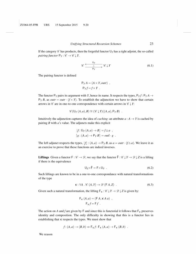
If the category C has products, then the forgetful functor UY has a right adjoint, the so-calledpairing functor PY : C → C ↓Y.
C C ↓Y⊥PY
UY
(6.1)
The pairing functor is defined
PY A = (A×Y,outr) ,
PY f = f×Y .
The functor PY pairs its argument with Y, hence its name. It respects the types, PY f : PY A→PY B, as outr = outr · (f× Y). To establish the adjunction we have to show that certainarrows in C are in one-to-one correspondence with certain arrows in C ↓Y:
C (UY (A,a),B)∼= (C ↓Y)((A,a),PY B) .
Intuitively the adjunction captures the idea of caching: an attribute a : A→ Y is cached bypairing B with a’s value. The adjuncts make this explicit
bf : UY (A,a)→ Bc= fMa ,
dg : (A,a)→ PY Be= outl · g .
The left adjunct respects the types, bfc : (A,a)→ PY B, as a = outr · (fMa). We leave it asan exercise to prove that these functions are indeed inverses.
Liftings Given a functor F : C →D , we say that the functor F̄ : C ↓Y→D ↓Z is a liftingif there is the equivalence
UZ ◦ F̄= F◦UY . (6.2)
Such liftings are known to be in a one-to-one correspondance with natural transformationsof the type
κ : ∀A . C (A,Y)→D (F A,Z) . (6.3)
Given such a natural transformation, the lifting Fκ : C ↓Y→D ↓Z is given by:
Fκ (A,a) = (F A,κ A a) ,
Fκ f = F f .
The action on A and f are given by F and since this is functorial it follows that Fκ preservesidentity and composition. The only difficulty in showing that this is a functor lies inestablishing that κ respects the types. We must show that
f : (A,a)→ (B,b)⇒ Fκ f : Fκ (A,a)→ Fκ (B,b) .
We reason

ZU064-05-FPR URS 15 September 2015 9:20
24 R. Hinze and N. Wu
κ B b · F f= { κ is natural }
κ A (b · f)= { assuming f : (A,a)→ (B,b) }
κ A a .
The fact that Fκ is a lifting follows directly from the definition. On objects we have:
UZ (Fκ (A,a)) = UZ (F A,κ A a) = F A = F (UZ (A,a)) ,
and on arrows:
UZ (Fκ f) = UZ (F f) = F f = F (UZ f) .
6.2 Zygomorphisms Revisited
A zygomorphism is a pair of morphisms x1 :µF→B1 and x2 :µF→B2, where the definitionof x1 depends on x2. The equations rely on algebras b1 : F (B1×B2)→B1 and b2 : FB2→B2,and are the solution to the following pair of equations:
x1 · in = b1 · F (x1 M x2) and x2 · in = b2 · F x2 . (6.4)
Our task is to show how we can express these two equations as a catamorphism in the slicecategory.
The definition of x1 relies on the existence of x2, and so intuitively we will needinformation to recover x2. The definition of x2 can be depicted by the following commutingtriangle:
F (µF) µF
B2
b2·F x2
in
x2
This motivates us to work with the slice category C ↓B2. The underlying functor that wehave to start with is F : C → C and we will lift this to a functor on the slice category whereF̄ :=Fκ is given by a natural transformation κ : ∀A . C (A,B2)→ C (F A,B2). Since wehave b2 at our disposal, the following suggests itself:
κ A (h : A→ B2) = b2 · F h . (6.5)
This definition conveniently gives us the equality
F̄ (µF,x2) = (F (µF),b2 · F x2) , (6.6)
and this corresponds to the left-hand-side of the commuting triangle above.

ZU064-05-FPR URS 15 September 2015 9:20
Unifying Structured Recursion Schemes 25
Now we can investigate the result of applying the canonical adjoint fold to the functor F̄.Instantiating Equation (5.8) with this data gives us:
UB2 (F̄ (µF,x2)) UB2 (F̄ (PB2 B))
UB2 ((µF,x2)) B
UB2 in
UB2 (F̄ bxc)
b1
x
⇐⇒F̄ (µF,x2) F̄ (PB2 B)
(µF,x2) PB2 B
in
F̄ bxc
bb1c
bxc
(6.7)
The diagram on the right is a catamorphism in the slice category. On the left hand side,we can unpack the definitions to reveal that x · in = b1 · F (xM x2) and this is precisely thedefining equation for the zygomorphism x1.
7 Unifying Recursion Schemes from Comonads
Recursion schemes from comonads (Uustalu et al., 2001), rsfcs for short, form a generalrecursion principle that makes use of a comonad N to provide ‘contextual information’ tothe algebra. This scheme covers a wide range of different morphisms from the zoo, but notall of them: nested datatypes are an example. In this section we will show how rsfcs are infact an instance of adjoint folds.
First, we introduce the relevant background to understand the construction of an rsfcin Section 7.1. The formal definition of an rsfc is then given in Section 7.2. We introduceEilenberg-Moore categories in Section 7.3, and bialgebras in Section 7.4 since these conceptswill be required to prove that rsfcs have a unique solution. This uniqueness is shown inSection 7.5 where an adjunction to the Eilenberg-Moore category is used to instantiate anadjoint fold.
7.1 Background: Comonads and Distributive Laws
Recursion schemes from monads make use of two concepts: comonads and distributive lawsover comonads. These concepts are presented in this section.
Comonads Functional programmers have embraced monads, and to a lesser extent, comon-ads, to capture effectful and context-sensitive computations. A comonad is a functorN : C → C equipped with natural transformations ε : N →̇ Id (counit), that extracts avalue from a context, and δ : N→̇N◦N (comultiplication), that duplicates a context, suchthat the following laws hold:
ε◦N · δ = N , (7.1a)
N◦ε · δ = N , (7.1b)
δ◦N · δ = N◦δ · δ . (7.1c)
The first two properties, the counit laws, state that duplicating a context and then discardinga duplicate is the same as doing nothing. The third property, the coassociative law, equatesthe two ways of duplicating a context twice. Monads (M,η,µ) are dual to comonads,with transformations η : Id→̇M (unit) and µ : M◦M→̇M (multiplication) that obey dualproperties.

ZU064-05-FPR URS 15 September 2015 9:20
26 R. Hinze and N. Wu
Distributive laws over comonads A distributive law λ : F◦N→̇N◦F of an endofunctor Fover a comonad N is a natural transformation satisfying the two coherence conditions:
ε◦F · λ = F◦ε , (7.2a)
δ◦F · λ = N◦λ · λ ◦N · F◦δ . (7.2b)
Distributing the comonad outside the functor and focusing is the same as focusing insidethe functor. Distributing the comonad outside the functor and duplicating is the same asduplicating inside the functor, and then distributing.
7.2 Recursion schemes from comonads
Just as with an adjoint fold, an rsfc is ‘doubly generic’: it is parametric in a datatype µF, andin a comonad N. As a particularly nice example, histomorphisms, the Squiggol renderingof course-of-values recursion, employ the cofree comonad, which makes available theresults of recursive calls on all subterms. (An even better choice is the cofree recursivecomonad (Uustalu & Vene, 2011), but this is outside the scope of this paper.) To this end itmakes use of a coalgebra fan : µF→ N (µF) that embeds a subterm in a context. For thecofree comonad, fan maps a term to the cotree of all subterms. The coalgebra can be definedgenerically in terms of a distributive law λ : F◦N→̇N◦F as detailed below.
Definition 7.1 (Comonadic recursion equation)Given a functor F, a comonad (N,ε,δ), a distributive law λ : F◦N→̇N◦F, and an algebrab : F (N B)→ B, a comonadic recursion equation in the unknown f : µF→ B has the form
f · in = b · F (N f · fan) , (7.3)
where fan = N in · λ (µF) : µF→ N (µF).
The composition N f · fan creates a context that makes the results of ‘recursive calls’ availableto the algebra b, which is a context-sensitive algebra—an (F◦N)-algebra, rather than merelyan F-algebra. Uustalu et al. (2001) showed the following
Theorem 7.2 (Rsfcs)The comonadic recursion equation (7.3) has the unique solution
f = ε B · N b · λ (N B) · F (δ B) .
A couple of remarks are in order. The recursion scheme involves both algebras andcoalgebras, and combines them in an interesting way. We noted above that fan is a coalgebra,but it is actually a bit more: it is a coalgebra for the comonad N. Furthermore, the algebra inand the coalgebra fan go hand-in-hand. They are related by the distributive law λ andform what is known as a λ -bialgebra, a combination of an algebra and a coalgebra with acommon carrier.
We postpone our proof of Theorem 7.2 to Section 7.5, after we have provided thenecessary background in Sections 7.3 and 7.4, which can be skipped by those alreadyfamiliar with the material.
When the cofree comonad is used to provide the contextual information for an rsfc, theensuing recursion scheme is a histomorphism (Uustalu et al., 2001). In Haskell, we can

ZU064-05-FPR URS 15 September 2015 9:20
Unifying Structured Recursion Schemes 27
represent the cofree comonad for a functor as:
data G∞ a = Cons∞ {head∞ :: a, tail∞ ::G (G∞ a)}
For the definition of the counit, we simply have ε = head∞. The comultiplication canbe given in terms of the so-called trace function, written - . This uses a coalgebra tocorecursively build a new level of the structure from a seed.
- :: Functor G⇒ (c→ G c)→ c→ G∞ cc = h where h = cons∞ · (idM fmap h · c)
A given seed is used to both populate the outer level of the structure, and as an argument tothe coalgebra that unpacks a new level of seeds, to which the trace is corecursively applied.We make use of cons∞, the uncurried version of Cons∞ to assemble these two parts. In effect,this is the fan that corresponds to a cofree comonad. The comultiplication is then simplyδ= tail∞ , where the seed is a cofree comonad, and the tail of its structure is recursivelyembedded. The trace can also be used to define a distributive law:
λ :: Functor G⇒ G (G∞ a)→ G∞ (G a)λ = fmap (fmap head∞) · fmap tail∞
This gives us all the ingredients we need to construct a histomorphism from an rsfc.
Example 7.3The knapsack function is an example of a histomorphism, where the underlying functor isNat, with constructors Zero and Succ. The algebra is given by knapsack, where we assumethat wvs :: [(N,R)] is implicitly supplied.
knapsack ::Nat (Nat∞ R)→ Rknapsack Zero = 0knapsack (Succ table) =
maximum0 [v+u | (w+1,v)← wvs,Just u← [lookup∞ table w ]]
This makes use of an auxiliary function lookup∞ that takes a table of type Nat∞ a of valuesindexed by natural numbers.
lookup∞ ::Nat∞ a→ N→Maybe alookup∞ (Cons∞ a m) 0 = Just alookup∞ (Cons∞ a Zero) (n+1) = Nothinglookup∞ (Cons∞ a (Succ table)) (n+1) = lookup∞ table n
This definition is given by induction on the naturals. In the base case, we simply retrievethe value at the head of table. Otherwise, we look deeper into the table: if the tail is empty,then the result is Nothing, since there are no more values to look up, otherwise, we recursedeeper into the table.
Putting the pieces together, we can obtain the following definition of knapsack:
knapsack :: N→ Rknapsack = head∞ · fmap knapsack · λ · fmap tail∞
While this construction corresponds to the interpretation of a histomorphism as an rsfc, itsuffers from the fact that the body of the fold involves applying the algebra to the result of a

ZU064-05-FPR URS 15 September 2015 9:20
28 R. Hinze and N. Wu
trace: its behaviour is quadratic. A little more work is required to derive a linear version,but the details are beyond the scope of this paper and covered fully by Hinze & Wu (2013).In short, we can collapse this into a fold that invokes the algebra only once per level.
7.3 Background: Eilenberg-Moore Categories
Coalgebras for a comonad A coalgebra for a comonad N is an N-coalgebra (C,c) thatrespects ε and δ:
ε C · c = idC , (7.4a)
δ C · c = N c · c . (7.4b)
If we first create a context and then focus, we obtain the original value. Creating a nestedcontext is the same as first creating a context and then duplicating it. For example, theso-called cofree coalgebra (N C,δ C) is respectful, which follows directly from (7.1b) and(7.1c). The second law (7.4b) also enjoys an alternative reading: c is a homomorphismof type (C,c) → (N C,δ C). This observation is at the heart of the Eilenberg-Mooreconstruction, which we discuss below. Coalgebras that respect ε and δ, and coalgebrahomomorphisms between them, form a category, known as the (co)-Eilenberg-Moorecategory and denoted CN. Eilenberg-Moore categories generalise categories of coalgebras:G-Coalg(C )∼= CN where N= G∞ is the cofree comonad.
Distributive laws and liftings We can use λ to colift F to the category CN. The coherenceconditions guarantee that Fλ : CN→ CN preserves respect for ε and δ. Dually, λ inducesthe lifting Nλ : F-Alg(C )→ F-Alg(C ). Now, the coherence conditions ensure that Nλ is acomonad with εa,A = ε A and δa,A = δ A. In particular, the lifted transformations ε : Nλ →̇ Id
and δ : Nλ →̇Nλ ◦Nλ are F-algebra homomorphisms.
Eilenberg-Moore construction As noted above, every adjunction generates a comonad.The converse is also true: every comonad N induces an adjunction that generates N—infact, in two canonical ways. One construction was discovered by Kleisli (1965), the otherby Eilenberg & Moore (1965). Here we need the latter, which constructs a right adjoint tothe forgetful functor UN : CN→ C .
C CN⊥CofreeN
UN
The functor CofreeN maps an object to the cofree coalgebra for N:
CofreeN B = (N B,δ B) , (7.5a)
CofreeN f = N f . (7.5b)
The counit ε : UN ◦CofreeN →̇ Id of the adjunction UN a CofreeN is the counit of N; the unitη : Id→̇CofreeN ◦UN, defined η (C,c) = c, extracts the action of a coalgebra, which is anN-coalgebra homomorphism of type (C,c)→ (N C,δ C) (7.4b). The bijection framed interms of the units reads:
f = ε B · UN h ⇐⇒ CofreeN f · η (C,c) = h ,

ZU064-05-FPR URS 15 September 2015 9:20
Unifying Structured Recursion Schemes 29
for all f : UN (C,c)→ B and h : (C,c)→ CofreeN B. The adjunction UN a CofreeN indeedgenerates the comonad N: we have UN ◦CofreeN = N and δ= UN ◦η◦CofreeN. Since UN
is faithful, we can simplify the bijection slightly:
f = ε B · h ⇐⇒ N f · c = h , (7.6)
for all f : C→ B and homomorphisms h : (C,c)→ (N B,δ B). Have we seen an arrow of theform N f · c before?
7.4 Background: Bialgebras
A bialgebra combines an algebra and a coalgebra with a common carrier. Bialgebras comein many flavours; we need the variant that combines F-algebras and coalgebras for acomonad N. The two functors have to interact coherently, described by a distributive law.
Bialgebras Let λ : F ◦N →̇N ◦ F be a distributive law for the endofunctor F over thecomonad N. A λ -bialgebra (a,X,c) consists of an F-algebra (a,X) and a coalgebra (X,c)for the comonad N such that the pentagonal law holds:
c · a = N a · λ X · F c . (7.7)
Loosely speaking, the law allows us to swap the algebra a and the coalgebra c. A λ -bialgebrahomomorphism is both an F-algebra and an N-coalgebra homomorphism. λ -bialgebras andtheir homomorphisms form a category, denoted λ -Bialg(C ).
The pentagonal law (7.7) also has two asymmetric renderings, which relate it to liftingsand coliftings.
F X F (N X)
X N X
a
F c
Nλ a
c
F X
F (N X)
X
N (F X)
N X
a
F c
λ X
c
N a
X F X
N X N (F X)
c
a
Fλ c
N a
(7.8)
The diagram on the left shows that c : (a,X)→ Nλ (a,X) is an F-algebra homomorphism.Dually, the diagram on the right identifies a : Fλ (X,c)→ (X,c) as an N-coalgebra homo-morphism. Thus, we can interpret the bialgebra (a,X,c) both as an algebra over a coalgebra(a,(X,c)), or as a coalgebra over an algebra ((a,X),c). Formally, we have the followingisomorphisms of categories:
Fλ -Alg(CN)∼= λ -Bialg(C )∼= (F-Alg(C ))Nλ . (7.9)
The alternative interpretations are useful to determine initial and final objects in λ -Bialg(C ).To determine the initial object, we use the ‘coalgebra over algebra’ view, as categories ofG-coalgebras have a trivial initial object: (0,0 G 0), where 0 is the initial object in theunderlying category and 0 G 0 the unique arrow from it. Consequently, (in,µF, fan) withfan = Nλ in is indeed initial.

ZU064-05-FPR URS 15 September 2015 9:20
30 R. Hinze and N. Wu
7.5 Recursion Schemes from Comonads are Adjoint Folds
We now return to the proof of Theorem 7.2 using our new vocabulary to derive the uniquesolution. Somewhat surprisingly, as an immediate consequence of this proof, it turns out thatrsfcs are an instance of adjoint folds, when previously, the two frameworks were thought ofas being orthogonal (Hinze, 2013). Of course, the derivation is not strictly necessary, but ithelps to relate the present development to prior work (Uustalu et al., 2001), and it hopefullyhelps to understand why rsfcs are an instance of adjoint folds. The development will followthe pattern we have already established.
First, we abstract away from the initial object (in,µF, fan), generalising to an arbitraryλ -bialgebra (a,A,c). The goal is to establish a bijection between arrows f : A→ B satisfyingf · a = b · F (N f · c) and λ -bialgebra homomorphisms h : (a,A,c)→ (b],N B,δ B), whereb] is a to-be-determined F-algebra. Now, we already know that arrows of type f : A→ B andN-coalgebra homomorphisms h : (A,c)→ (N B,δ B) are in one-to-one correspondence (7.6).So we identify N f · c as the transpose of f and simplify f’s equation to f · a = b · F h. Itremains to show that h is an F-algebra homomorphism of type (a,A)→ (b],N B).
F A F (N B)
A B
F h
a b
f
⇐⇒F A F (N B)
A N B
F h
a b]
h
(7.10)
The strategy for the proof is clear: we have to transmogrify f into N f · c. Thus, we apply N
to both sides of f · a = b · F h and then ‘swap’ a and c using the pentagonal law (7.7).
f · a = b · F h=⇒ { N functor }
N f · N a = N b · N (F h)=⇒ { Leibniz }
N f · N a · Fλ c = N b · N (F h) · Fλ c⇐⇒ { a : Fλ (A,c)→ (A,c) is an N-coalgebra homomorphism (7.8) }
N f · c · a = N b · N (F h) · Fλ c⇐⇒ { N f · c = h }
h · a = N b · N (F h) · Fλ c⇐⇒ { F h = Fλ h : Fλ (A,c)→ Fλ (N B,δ B) is an N-coalgebra homomorphism (7.8) }
h · a = N b · Fλ (δ B) · F h
The proof makes essential use of the pentagonal law (7.7), the fact that a and h are N-coalgebra homomorphisms, and that Fλ preserves N-coalgebra homomorphisms. Along theway, we have derived a formula for b]:
b] = N b · Fλ (δ B) = N b · λ (N B) · F (δ B) . (7.11)
We have to show that (b],N B,δ B) is a λ -bialgebra. Since Fλ (N B,δ B) is a coalgebra forthe comonad N, we can conclude using (7.6) that b] is a coalgebra homomorphism of typeFλ (N B,δ B)→ (N B,δ B), which establishes the desired result. Furthermore b = ε B · b],

ZU064-05-FPR URS 15 September 2015 9:20
Unifying Structured Recursion Schemes 31
which allows us to complete the proof.
h · a = b] · F h=⇒ { Leibniz }
ε B · h · a = ε B · b] · F h⇐⇒ { f = ε B · h and b = ε B · b] }
f · a = b · F h
We have discovered an important fact: b and b] are also related by the Eilenberg-Mooreadjunction UN a CofreeN since b] = bbc! Using the notation for adjuncts, the right-handside of (7.10) reads bfc · a = bbc · F bfc. This looks suspiciously like the right-hand sideof (5.8), which relates trahos (adjoint folds) and homomorphisms. However, the originalequation for f does not seem to fit into the picture. This is because it omits the forgetfulfunctor UN. If we make it explicit, we obtain the following bijection, which is indeed aninstance of (5.8).
UN (Fλ (A,c)) UN (Fλ (CofreeN B))
UN (A,c) B
UN a
UN (Fλ bfc)
b
f
⇐⇒
Fλ (A,c) Fλ (CofreeN B)
(A,c) CofreeN B
a
Fλ bfc
bbc
bfc
If we simplify the composition of functors using UN ◦Fλ = F◦UN and UN ◦Fλ ◦CofreeN =
F◦UN ◦CofreeN = F◦N, we obtain the original equivalence (7.10). The somewhat pedanticdiagrams above explicate all the information that is implicit. For example, we can read offthat a is an N-coalgebra homomorphism.
The second step should be routine by now. If we instantiate (a,A,c) to the initial λ -bialgebra (in,µF, fan), we obtain that the unique solution of the original equation (7.3) isf = d bbc e or, expressed using the vocabulary of (Uustalu et al., 2001), f = ε B · b] . Werecord
Theorem 7.4
Let N : C → C and F : C → C be endofunctors. A recursion scheme from the comonad N
and the distributive law λ : F◦N→̇N◦F can be framed as a canonical adjoint fold basedon the Eilenberg-Moore adjunction UN a CofreeN. The data functor for the adjoint fold isFλ : CN→ CN, the canonical control functor is UN ◦Fλ ◦CofreeN = F◦N, and the algebraremains b : F (N B)→ B.
C CN⊥CofreeN
F◦NUN
Fλ
Let us conclude the section by investigating an alternative control functor: since UN◦Fλ =
F◦UN, the functor F itself can be used as the control! For this case the distributive law σ isan isomorphism, even an identity, so we can invoke the machinery of Section 5.6 and lift theadjunction UN a CofreeN to an adjunction between categories of algebras. The conjugateof σ= id is just λ , we have UN ◦τ= λ . (The coherence condition (7.2b) shows that λ is an
ZU064-05-FPR URS 15 September 2015 9:20
32 R. Hinze and N. Wu
N-coalgebra homomorphism of type Fλ ◦CofreeN →̇CofreeN ◦F.)
F-Alg(C ) Fλ -Alg(CN)
C CN
⊥CofreeτN
UFa ∼=
UidN
UFλa
⊥CofreeN
F
FreeF
UN
Fλ
FreeFλ
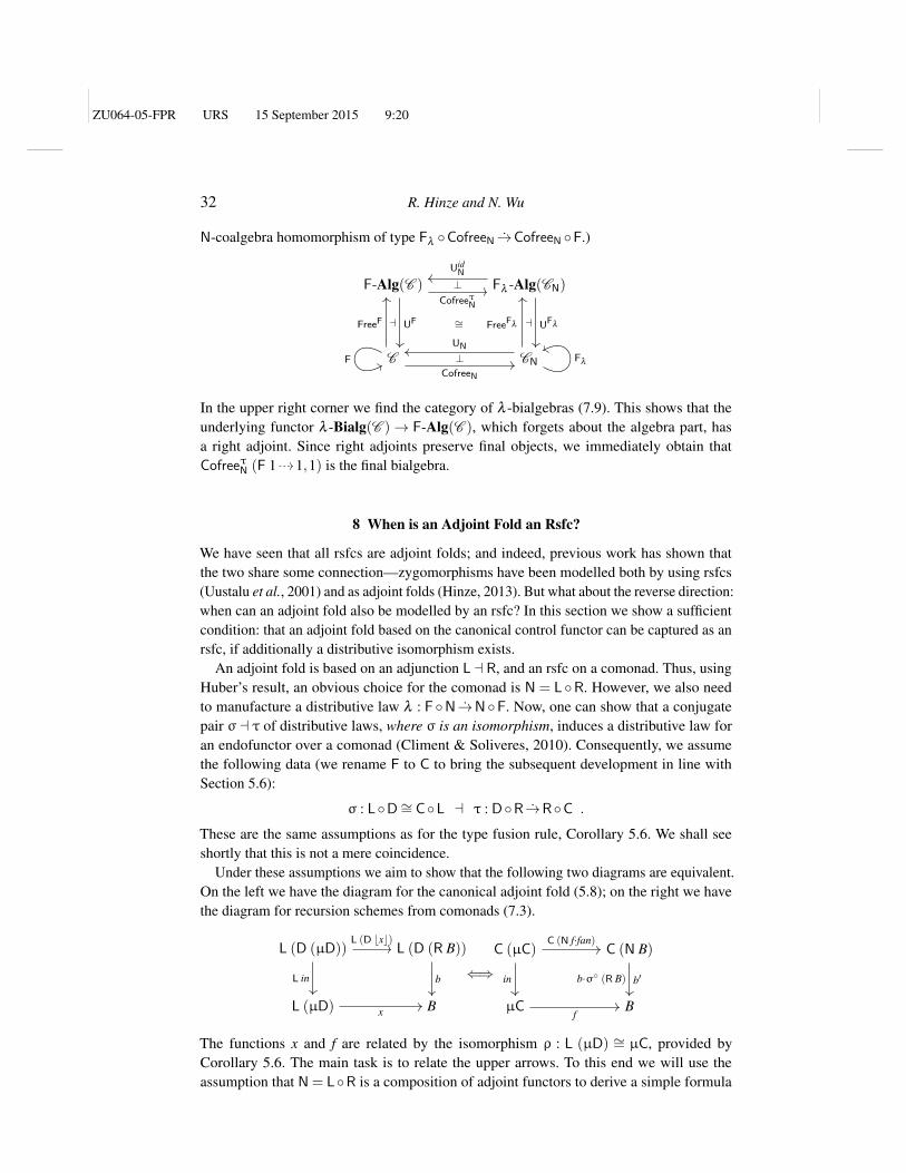
In the upper right corner we find the category of λ -bialgebras (7.9). This shows that theunderlying functor λ -Bialg(C )→ F-Alg(C ), which forgets about the algebra part, hasa right adjoint. Since right adjoints preserve final objects, we immediately obtain thatCofreeτN (F 1 1,1) is the final bialgebra.
8 When is an Adjoint Fold an Rsfc?
We have seen that all rsfcs are adjoint folds; and indeed, previous work has shown thatthe two share some connection—zygomorphisms have been modelled both by using rsfcs(Uustalu et al., 2001) and as adjoint folds (Hinze, 2013). But what about the reverse direction:when can an adjoint fold also be modelled by an rsfc? In this section we show a sufficientcondition: that an adjoint fold based on the canonical control functor can be captured as anrsfc, if additionally a distributive isomorphism exists.
An adjoint fold is based on an adjunction L a R, and an rsfc on a comonad. Thus, usingHuber’s result, an obvious choice for the comonad is N = L ◦R. However, we also needto manufacture a distributive law λ : F◦N→̇N◦F. Now, one can show that a conjugatepair σ a τ of distributive laws, where σ is an isomorphism, induces a distributive law foran endofunctor over a comonad (Climent & Soliveres, 2010). Consequently, we assumethe following data (we rename F to C to bring the subsequent development in line withSection 5.6):
σ : L◦D∼= C◦L a τ : D◦R→̇R◦C .
These are the same assumptions as for the type fusion rule, Corollary 5.6. We shall seeshortly that this is not a mere coincidence.
Under these assumptions we aim to show that the following two diagrams are equivalent.On the left we have the diagram for the canonical adjoint fold (5.8); on the right we havethe diagram for recursion schemes from comonads (7.3).
L (D (µD)) L (D (R B))
L (µD) B
L in
L (D bxc)
b
x
⇐⇒C (µC) C (N B)
µC B
C (N f·fan)
in b′b·σ◦ (R B)
f
The functions x and f are related by the isomorphism ρ : L (µD) ∼= µC, provided byCorollary 5.6. The main task is to relate the upper arrows. To this end we will use theassumption that N= L◦R is a composition of adjoint functors to derive a simple formula

ZU064-05-FPR URS 15 September 2015 9:20
Unifying Structured Recursion Schemes 33
for fan : µC→ N (µC) by working instead with fan′ : L (µD)→ N (L (µD)), related byfan = N ρ · fan′ · ρ◦.
But first, we have to set up the infrastructure. From the data above we can generate twodistributive laws (Climent & Soliveres, 2010):
α = τ−σ◦ = R◦σ◦ · τ◦L : D◦M→̇M◦D , (8.1a)
γ = σ◦−τ = L◦τ · σ◦ ◦R : C◦N→̇N◦C . (8.1b)
The distributive law γ satisfies the two requirements for λ (7.2) (note that Nγ = Lσ◦ ◦Rτ);
the distributive law α of an endofunctor over a monad enjoys analogous conditions:
α · D◦η = η◦D , (8.2a)
α · D◦µ = µ◦D · M◦α · α◦M . (8.2b)
Next we construct an initial γ-bialgebra. Since Lσ◦
: D-Alg(D)→ C-Alg(C ) is leftadjoint (5.13), and left adjoints preserve initial objects (3.8a), we know that Lσ
◦(in,µD) =
(Lσ◦
in,L (µD)) is initial in C-Alg(C ). To determine a formula for fan′, the correspondingcoalgebra part, we have to delve a bit deeper into the theory. The Eilenberg-Moore adjunctionUN a CofreeN has an important property: it is the largest adjunction that generates N, inthe sense that for every adjunction L a R there is a unique adjoint square from L a R toUN a CofreeN, depicted in the diagram below. (Since the distributive laws of the adjointsquare are identities, it is actually a so-called map of adjunctions.)
C C
D CN
Ra CofreeNa
E
L UN
The so-called comparison functor E : D → CN is defined
E A = (L A,L (η A)) , (8.3a)
E f = L f . (8.3b)
Since the distributive laws of the adjoint square are identities, we have UN ◦E= Id◦L andE◦R= CofreeN ◦ Id.
Note that the carrier of E A is L A, which suggests that the coalgebra part of the initialγ-bialgebra is perhaps just L (η (µD)). Then it remains to verify that Lσ
◦in and L (η (µD))
satisfy the pentagonal law. We prove, in fact, a slightly more general result: we show that(Lσ
◦a,L A,L (η A)) is a γ-bialgebra, where (a,A) : D-Alg(D) is an arbitrary D-algebra, by
lifting the comparison functor E to categories of algebras with a distributive law, as in thediagram below.
D-Alg(D) Cγ-Alg(CN)
D CN
Eθ
UD UCγ
E

ZU064-05-FPR URS 15 September 2015 9:20
34 R. Hinze and N. Wu
To this end, we need a distributive law θ : E◦D←̇Cγ ◦E. We claim that σ◦ itself fits thebill: UN ◦θ = σ◦. (Note that UN ◦E ◦D ←̇UN ◦Cγ ◦E = L ◦D ←̇C ◦L). In other words,we have to show that σ◦ is a natural N-coalgebra homomorphism of type E◦D←̇Cγ ◦E.Plugging in the definitions, we reason
L◦η◦D · σ◦
= { α respects η (8.2a) }L◦α · L◦D◦η · σ◦
= { σ◦ is natural }L◦α · σ◦ ◦M · C◦L◦η
= { σ◦−α= σ◦−τ−σ◦ = γ−σ◦ }N◦σ◦ · γ◦L · C◦L◦η .
We have established that fan′ = L (η (µD)), and so an attractive definition of fan emerges:
fan = N ρ · L (η (µD)) · ρ◦ , (8.4)
which is in most cases a much more efficient implementation than N in · λ (µF) .We are now ready to show that adjoint folds are recursion schemes from comonads,
provided that a distributive isomorphism σ : L◦D∼= C◦L exists. Here is the diagram forrsfcs with applications of the isomorphism σ made explicit.
L (D (µD)) C (L (µD)) C (N B) L (D (R B))
L (µD) L (µD) B B
σ (µD)
L in
C (N x·fan′)
Lσ◦
in b·σ◦ (R B)
σ◦ (R B)
b
x
Thus, it remains to show that L bxc= N x · fan′.
L bxc= { b−c expressed in terms of η; (3.4a) with k, f,h := x, id, id }
L (R x · η (µD))
= { L functor }L (R x) · L (η (µD))
= { definition of N and fan′ (8.4) }N x · fan′
We record the result in the following
Theorem 8.1Let x : L (µD)→ B be a canonical adjoint fold based on the adjunction L a R : C ⇀ D withconjugates σ a τ where σ is an isomorphism, a data functor D : D →D , a control functorC : C →C , and an algebra b :C B→ B. Since σ is an isomorphism we have ρ : L (µD)∼=µC.The adjoint fold x can be framed in terms of a recursion scheme f : µC→ B for the comonadN= L◦R, where x = f · ρ. The distributive law for the rsfc is λ = σ◦−τ : C◦N→̇N◦C,and its algebra is b · σ◦ (R B) : C (N B)→ B.

ZU064-05-FPR URS 15 September 2015 9:20
Unifying Structured Recursion Schemes 35
Example 8.2Mutumorphisms are an instance of rsfcs using σ = id : ∆ ◦D = D2 ◦∆, see Example 5.7.Since the isomorphism is an identity, we can transform the diagram for adjoints folds almostdirectly into a corresponding diagram for rsfcs (A :=µD).
∆ (D A) ∆ (D ((×) B))
∆ A B
∆ in
∆ (D bxc)
b
x
⇐⇒D2 (∆ A)) D2 (∆ ((×) B))
∆ A B
∆ in
D2 (∆ bxc)
b
x
In the upper right corner we discover the comonad N= ∆◦ (×), which works over a productcategory. As fan′ = ∆ (idM id), we have ∆ bxc = ∆ ((×) x · (idM id)) = N x · fan′. If weidentify ∆ (µD) and µD2 so that ∆ in = in, the diagram for rsfcs emerges.
We have seen in the previous section that an rsfc (based on a comonad N and a distributivelaw λ : F◦N→̇N◦F) can be framed as an adjoint fold using the Eilenberg-Moore adjunctionUN a CofreeN. Now, what happens if we go round in a circle, instantiating the developmentabove to D= Fλ , C= F, and id : UN ◦Fλ = F◦UN? Recall that UN ◦τ= λ ; consequently,
γ = σ◦−τ = UN ◦τ · id◦ ◦CofreeN = λ .
Hence, we obtain back the original rsfc!We have seen that mutumorphisms based on ∆ a (×) can be modelled by using an rsfc.
Of course, this does not work for every adjunction. As an example, consider the curryadjunction. One would need a control functor C such that:
σ : (−×P)◦D∼= C◦ (−×P) .
Such a control functor is not guaranteed to exist for all datatypes.
9 Monadic Catamorphisms
So far we have devoted our attention to the (co)Eilenberg-Moore adjunction, since itsconstruction on comonads has allowed us to relate adjoint folds to rsfcs. A connected lineof work is to investigate the Kleisli adjunction. Its construction on monads allows us torelate adjoint folds to yet another recursion scheme: monadic catamorphisms (Fokkinga,1994). This scheme allows monadic computations to be threaded through the traversal of arecursive structure. But first we review the construction of the Kleisli adjunction.
9.1 Background: Kleisli Categories
The Kleisli category Given a category C and a monad M : C → C , we can construct theKleisli category, written CM. This category imposes further structure on C by incorporatinga monadic value to the target of every arrow. The objects in CM are the same as those in C ,but the arrows differ. A Kleisli arrow A→ B : CM is a C -arrow of type A→M B : C . Theidentity arrow of an object X : CM is the component η X : X→M X of the unit of the monad.The composition of arrows f : A→M B : C and g : B→M C : C in the Kleisli category isgiven by g / f : A→M C : C , where g / f = µ C ·M g · f.

ZU064-05-FPR URS 15 September 2015 9:20
36 R. Hinze and N. Wu
The Kleisli adjunction It is easy to show that the categories C and CM are related by anadjoint pair of functors LM and RM:
CM C⊥RM
LM
.
The functor LM promotes arrows of the base category to “pure” Kleisli arrows:
LM A = A , (9.1a)
LM f = η B · f , (9.1b)
where f : A→ B : C .The functor RM maps objects in the Kleisli category to monadic objects in the underlying
category:
RM A =M A , (9.2a)
RM f = µ B ·M f , (9.2b)
where the arrow f : A→M B : C is first lifted so that its source matches the expected object,and then ‘rebalanced’ by the multiplication µ : M◦M→̇M of the monad.
The unit η : Id→̇RM ◦LM of this adjunction is simply the unit of the monad M, and thecounit ε : LM ◦RM →̇ Id is the identity idM. A rather curious property of this adjunction isthat the adjuncts merely cast arrows between the categories, where bfc= f and dge= g, ascan be easily verified.
Liftings A lifting of the functor F : C → C is a functor F̄ : CM→ CM such that
LM ◦F= F̄◦LM . (9.3)
Recall that a distributive law λ : F◦M→̇M◦F of an endofunctor F over a monad M is anatural transformation satisfying the two coherence conditions described by Equations (8.2a)and (8.2b). We can use such a distributive law to produce the lifting Fλ : CM→ CM:
Fλ A = F A , (9.4a)
Fλ f = λ B · F f , (9.4b)
where f : A→M B : C . Beware that this notation overlaps with that of coliftings to functorsover coalgebras, which we will not use in this section.
The proof that this is a lifting makes use of the distributive law:
LM (F f)= { definition of LM (9.1b) }
η (F B) · F f= { distributive law (8.2a) }
λ B · F (η B) · F f= { F functor and definition of Fλ (9.4b) }
Fλ (η B · f)= { definition of LM (9.1b) }
Fλ (LM f)

ZU064-05-FPR URS 15 September 2015 9:20
Unifying Structured Recursion Schemes 37
The lifting induces the conjugate id : LM ◦ F ∼= Fλ ◦ LM, such that id a τ. Using Equa-tion (3.12b) we can show that λ = τ ◦LM. Since LM is the identity on objects these twonatural transformations have the same components.
9.2 Monadic catamorphisms are adjoint folds
A monadic catamorphism threads a computation through some recursive structure. Moreformally, the scheme is defined by the following equation:
Definition 9.1 (Monadic catamorphism equation)Given a functor F : C → C , a monad (M,η,µ), a distributive law λ : F◦M→̇M◦F, andan algebra b : F B→ B : CM, a monadic catamorphism in the unknown x : LM (in,µF)→LM (b,B) has the form
x / LM in = b / Fλ x , (9.5)
where the functor Fλ : CM→ CM is the lifting of F by λ .
The machinery we have set up earlier on in this section allows us to show how thisdefinition corresponds to an adjoint fold. We have the following situation:
CM C⊥RM
Fλ
LMF ,
where Fλ is the lifting of F using a given distributive law λ : F◦M→̇M◦F.Given an algebra b : Fλ B→ B, we can apply our definitions to Equation (5.12) to yield:
Fλ (LM (µF)) Fλ B
LM (µF) B
Lid◦M in
Fλ x
b
x
⇐⇒F (µF) F (RM B)
µF RM B
in
F bxc
RτM b
bxc
The diagram on the left is in the Kleisli category, and corresponds directly to Equation (9.5).The diagram on the right is a fold f = bxc : µF→M B that involves only the base categoryC . Some calculation gives us a clearer implementation:
f · in = RτM b · F f
⇐⇒ { definition of lifting (3.1a) }f · in = RM b · τ B · F f
⇐⇒ { definition of RM b (9.2b) }f · in = µ B ·M b · τ B · F f
This is precisely the characterization given by Fokkinga (1994).
Example 9.2The function accumulate from Section 2 is a monadic fold where the underlying functor isList and the distributive law is λ : List◦M→̇M◦List, for an arbitrary monad M. In Haskell,

ZU064-05-FPR URS 15 September 2015 9:20
38 R. Hinze and N. Wu
we can implement this law as:
λ :: (Functor m,Monad m)⇒ List a (m x)→ m (List a x)λ Nil = return Nilλ (Cons a mx) = mx>>=λx→ return (Cons a x)
The proof that this law respects the unit and multiplication of the monad is a simple exercise.We are in a position to give a definition that matches the structure of a monadic fold,
bearing in mind that τ and λ agree on their components:
accumulate :: (Functor m,Monad m)⇒ [m x ]→ m [x]accumulate = join · fmap b · λ
where b Nil = return [ ]
b (Cons mx xs) = mx>>=λx→ return (x : xs)
On non-empty input, the algebra b ::List (m x) [x]→ m [x] appends the tail of results to thehead of the list within a monadic context.
10 Calculational Properties
The calculational properties of adjoint folds were studied at depth in (Hinze, 2013). Giventhat rsfcs are an instance of adjoint folds, a natural question to ask is how this correspondsto the properties introduced alongside recursion schemes from comonads (Uustalu et al.,2001). We start by listing the properties of adjoint folds.
Uniqueness Property The uniqueness property underpins many of the other laws, andintroduces the notation b L to represent the unique solution to the adjoint fold equationgiven by Theorem 5.2.
x = b L ⇐⇒ x · L in = b · C x · σ (µD) . (10.1)
Computation Law An immediate consequence of the uniqueness property is the compu-tation law, which simply arises by substituting the unique solution b L into the definingequation for adjoint folds:
b L · L in = b · C b L · σ (µD) . (10.2)
Reflection Law The reflection law arises when we substitute id for x in the uniquenessproperty:
id = b L ⇐⇒ L in = b · σ (µD) . (10.3)
Example 10.1 (Catamorphisms)We can bring these properties back to familiar territory by instantiating Equation (10.1) tothe adjunction Id a Id, since this gives rise to standard folds, where the canonical controlfunctor is C= Id◦D◦ Id=D, and σ is simply the identity. In this setting, the uniquenesslaw is rendered:
x = b ⇐⇒ x · in = b · x .

ZU064-05-FPR URS 15 September 2015 9:20
Unifying Structured Recursion Schemes 39
The computation law becomes the following, which is sometimes also referred to ascancellation:
b · in = b · D b (10.4)
The standard reflection law arises out of substituting the right hand side into the left:
id = b ⇐⇒ in = b
Example 10.2 (Recursion schemes from comonads)
We have already seen that recursion schemes from comonads are an instance of adjointfolds where the adjunction is UG a CofreeG, the data functor is Fλ , and the control functoris the canonical one. As can be expected, specializing the calculational properties aboveleads to the properties of rsfcs introduced by Uustalu et al. (2001).
For example, we can show that the computation law is in fact a generalized versionof what was originally called the cancellation law. This is a simple case of plugging indefinitions when the computation law for the canonical control functor is used:
b UN· UN in = b · UN (Fλ (CofreeN b UN
· η (µFλ )))
⇐⇒ { definition of UN }b UN
· in = b · Fλ (CofreeN b UN· η (µFλ ))
⇐⇒ { definition of Fλ (3.2b) }b UN
· in = b · F (CofreeN b UN· η (µFλ ))
⇐⇒ { definition of CofreeN (7.5b) }b UN
· in = b · F (N b UN· η (µFλ ))
⇐⇒ { definition of fan (8.4) }b UN
· in = b · F (N b UN· fan)
Thus we have arrived at the comonadic recursion equation (7.3), and shown that it is solveduniquely by b UN
.We can also reason that folding with the algebra b = in · F (ε (µF)) is the identity, which
follows by showing that the right hand side of the reflection law is true.
id = in · (F◦ε) (µF) UN
⇐⇒ { reflection law (10.3) }UN in = in · (F◦ε) (µF) · (UN ◦Fλ ◦η) (µFλ )
⇐⇒ { definition of UN and µFλ = (µF, in) }UN in = UN in · (F◦ε◦UN) (µFλ ) · (UN ◦Fλ ◦η) (µFλ )
⇐⇒ { Fλ is a colifting }UN in = UN in · (F◦ε◦UN) (µFλ ) · (F◦UN ◦η) (µFλ )
⇐⇒ { functoriality of F }UN in = UN in · F ((ε◦UN) (µFλ ) · (UN ◦η) (µFλ ))
⇐⇒ { triangle identity (3.5a) }UN in = UN in
Example 10.3 (Catamorphisms as recursion schemes from comonads)

ZU064-05-FPR URS 15 September 2015 9:20
40 R. Hinze and N. Wu
Using the uniqueness property for rsfcs, we can show how to express catamorphisms asrsfcs.
b Id = b · F (ε B) UN
⇐⇒ { uniqueness property (10.1) }b Id · UN in = b · F (ε B) · (UN ◦Fλ ◦CofreeN) b Id · (UN ◦Fλ ◦η) (µFλ )
⇐⇒ { Fλ is a colifting }b Id · UN in = b · F (ε B) · (F◦UN ◦CofreeN) b Id · (F◦UN ◦η) (µFλ )
⇐⇒ { functoriality of F }b Id · UN in = b · F (ε B · (UN ◦CofreeN) b Id · (UN ◦η) (µFλ ))
⇐⇒ { naturality of ε }b Id · UN in = b · F ( b Id · ε (µF) · (UN ◦η) (µFλ ))
⇐⇒ { definition of UN }b Id · in = b · F ( b Id · (ε◦UN) (µFλ ) · (UN ◦η) (µFλ ))
⇐⇒ { triangle identity (3.5a) }b Id · in = b · F b Id
This shows that every catamorphism is an rsfc. Or else, we can view this as a simple programoptimization: an rsfc whose algebra ignores the comonadic context and merely extracts avalue can be simplified to become a catamorphism.
10.1 Fusion
A useful set of laws involve the fusion of a fold with some arrow to produce a different fold.
Fusion Law The simplest instance of fusion, which we simply call the fusion law, givesthe conditions required to fuse an arrow that follows after an adjoint fold.
Given an adjoint fold a L : C (L (µD),A), and an arrow h : C (A,B), we can form a newadjoint fold b L : C (L (µD) B) under certain conditions, which we can calculate:
h · a L = b L
⇐⇒ { uniqueness property (10.1) }h · a L · L in = b · C (h · a L · σ (µD)
⇐⇒ { computation (10.2) }h · a · C a L · σ (µD) = b · C (h · a L) · σ (µD)
⇐⇒ { functoriality of C }h · a · C a L · σ (µD) = b · C h · C a L · σ (µD)
⇐= { Leibniz law }h · a = b · C h
Summarizing, we can state the fusion law as follows:
h · a L = b L ⇐= h · a = b · C h . (10.5)
The arrow is required to be a C-homomorphism.
Conjugate Fusion Law The fusion law focuses on creating a new fold whose codomain isa modification of the original. Another form of fusion of interest is the so-called conjugate

ZU064-05-FPR URS 15 September 2015 9:20
Unifying Structured Recursion Schemes 41
fusion law, which focuses instead on generating a fold whose domain differs. This time, weprecompose the fold b′ L by a conjugate α : L→̇L′. It is instructive to derive the conditionsrequired for this situation:
b L′ · α (µD) = b L
⇐⇒ { uniqueness property (10.1) }b L′ · α (µD) · L in = b · C ( b L′ · α (µD)) · σ (µD)
⇐⇒ { naturality of α : L→̇L′ }b L′ · L
′ in · α (D (µD)) = b · C ( b L′ · α (µD)) · σ (µD)
⇐⇒ { computation law (10.2) }b · C b L′ · σ
′ (µD) · α (D (µD)) = b · C ( b L′ · α (µD)) · σ (µD)
⇐⇒ { functoriality of C }b · C b L′ · σ
′ (µD) · α (D (µD)) = b · C b L′ · C (α (µD)) · σ (µD)
⇐= { Leibniz law }σ′ (µD) · α (D (µD)) = C (α (µD)) · σ (µD)
We have shown that the precomposition of α with fold yields another, so long as theconjugates of the fold are related by α:
b L′ · α (µD) = b L ⇐= σ′ · α◦D= C◦α · σ . (10.6)
A natural transformation that satisfies the property on the right is sometimes called atransformation of conjugates.
General Fusion The previous two laws are an instance of a more general fusion lawwhere we transform both domain and codomain at once using a natural transformationα : C (L−,B)→̇C ′ (L′ −,B′). We can calculate the required conditions as follows:
α (µD) b L = b′ L′
⇐⇒ { uniqueness property (10.1) }α (µD) b L · L
′ in = b′ · C′ (α (µD) b L) · σ′ (µD)
⇐⇒ { naturality of α }α (D (µD)) ( b L · L in) = b′ · C′ (α (µD) b L) · σ
′ (µD)
⇐⇒ { computation law (10.2) }α (D (µD)) (b · C b L · σ (µD)) = b′ · C′ (α (µD) b L) · σ
′ (µD)
⇐= { abstraction }α (D X) · (λx . b · C x · σ X) = (λx . b′ · C′ x · σ′ X) · α X
We can recover the fusion law by applying a transformation that postcomposes withh : C (A,B), which is natural in its domain: h · − : C (L−,A)→̇C (L−,B). Instantiatingthis to the general fusion law gives:
(h · −) (D X) · (λx . a · C x · σ X) = (λx . b · C x · σ X) · (h · −) X⇐⇒ { extensionality }
∀x . h · a · C x · σ X = b · C (h · x) · σ X⇐⇒ { functoriality of C }
∀x . h · a · C x · σ X = b · C h · C x · σ X⇐= { Leibniz }
h · a = b · C h
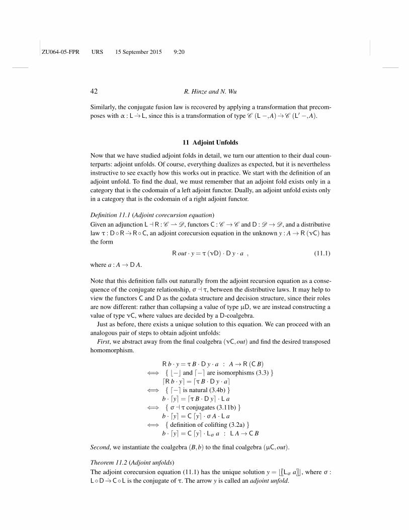
ZU064-05-FPR URS 15 September 2015 9:20
42 R. Hinze and N. Wu
Similarly, the conjugate fusion law is recovered by applying a transformation that precom-poses with α : L→̇L, since this is a transformation of type C (L−,A)→̇C (L′ −,A).
11 Adjoint Unfolds
Now that we have studied adjoint folds in detail, we turn our attention to their dual coun-terparts: adjoint unfolds. Of course, everything dualizes as expected, but it is neverthelessinstructive to see exactly how this works out in practice. We start with the definition of anadjoint unfold. To find the dual, we must remember that an adjoint fold exists only in acategory that is the codomain of a left adjoint functor. Dually, an adjoint unfold exists onlyin a category that is the codomain of a right adjoint functor.
Definition 11.1 (Adjoint corecursion equation)Given an adjunction L a R : C ⇀D , functors C : C → C and D : D→D , and a distributivelaw τ : D◦R→̇R◦C, an adjoint corecursion equation in the unknown y : A→ R (νC) hasthe form
R out · y = τ (νD) · D y · a , (11.1)
where a : A→ D A.
Note that this definition falls out naturally from the adjoint recursion equation as a conse-quence of the conjugate relationship, σ a τ, between the distributive laws. It may help toview the functors C and D as the codata structure and decision structure, since their rolesare now different: rather than collapsing a value of type µD, we are instead constructing avalue of type νC, where values are decided by a D-coalgebra.
Just as before, there exists a unique solution to this equation. We can proceed with ananalogous pair of steps to obtain adjoint unfolds:
First, we abstract away from the final coalgebra (νC,out) and find the desired transposedhomomorphism.
R b · y = τ B · D y · a : A→ R (C B)⇐⇒ { b−c and d−e are isomorphisms (3.3) }
dR b · ye= dτ B · D y · ae⇐⇒ { d−e is natural (3.4b) }
b · dye= dτ B · D ye · L a⇐⇒ { σ a τ conjugates (3.11b) }
b · dye= C dye · σ A · L a⇐⇒ { definition of colifting (3.2a) }
b · dye= C dye · Lσ a : L A→ C B
Second, we instantiate the coalgebra (B,b) to the final coalgebra (µC,out).
Theorem 11.2 (Adjoint unfolds)The adjoint corecursion equation (11.1) has the unique solution y = b Lσ a c, where σ :L◦D→̇C◦L is the conjugate of τ. The arrow y is called an adjoint unfold.

ZU064-05-FPR URS 15 September 2015 9:20
Unifying Structured Recursion Schemes 43
(a) catamorphism (Hagino, 1987; Malcolm, 1990b) Id a Id depthmutumorphism (Fokkinga, 1990) ∆ a (×) even/odd
special case: zygomorphism (Malcolm, 1990a) UY a PY perfectspecial case: paramorphism (Meertens, 1992) wc
fold with a parameter (Pardo, 2002) −×P a (−)P cat, depthsgeneralised fold (Bird & Paterson, 1999) (−◦F) a RanF totalrecursion scheme from a comonad (Uustalu et al., 2001) UN a CofreeN
special case: histomorphism (Uustalu & Vene, 1999b) knapsackmonadic catamorphism (Fokkinga, 1994) LM a RM accumulate
(b) anamorphism (Hagino, 1987; Malcolm, 1990b) Id a Id from(mutumorphism) (+) a ∆
special case: apomorphism (Vene & Uustalu, 1998) insert(generalised unfold) LanF a (−◦F)λ -coiteration (Bartels, 2003) FreeM a UM
special case: futumorphism (Uustalu & Vene, 1999b)
Table 1. Adjoint folds (a) and unfolds (b); LanP and RanP are left and right Kan extensions,FreeM a UM is the Eilenberg-Moore adjunction, and LM a RM is the Kleisli adjunction.
ProofThis is an immediate consequence of finality.
R out · y = τ (νD) · D y · a⇐⇒ { see above }
out · dye= C dye · Lσ a⇐⇒ { (νC,out) final }
dye= Lσ a⇐⇒ { b−c and d−e are isomorphisms (3.3) }
x = b Lσ a c
The adjoint unfolds formulation allows us to bring all of the corecursive schemes mentionedin Section 2 into a single framework. The procedure is much the same as for the recursivecounterparts we have covered: the hard part is identifying the adjunction that needs to beinstantiated. We do not go through the details in this paper, but a summary of the adjointunfolds and their corresponding instantiations are to be found in Table 1.
12 Related Work
Adjoint folds Mendler-style adjoint folds first appeared in a paper by Bird & Paterson(1999), where they were used to show that generalised folds are uniquely defined. (Somewhatironically, adjoint folds were only used in the proofs, not as a general recursion principle.)The algebraic variant of adjoint folds that we have employed throughout was introducedby Matthes & Uustalu (2004) under the name generalised iteration. The first author ofthe present paper explored the design space of adjoint folds (Hinze, 2013), identifying theadjunctions underlying various recursion schemes. The paper also shows how to combinerecursion schemes by combining the underlying adjunctions. Alas, he wrote “However, we

ZU064-05-FPR URS 15 September 2015 9:20
44 R. Hinze and N. Wu
cannot reasonably expect that adjoint (un)folds subsume all existing species of morphisms.For instance, a largely orthogonal extension of standard folds are recursion schemes fromcomonads.”
Recursion schemes from comonads Recursion schemes from comonads are due to Uustaluet al. (2001). Simultaneously and independently, Bartels (2003) introduced the dual con-struction under name λ -coiteration. Technically, his work is closest to ours in the use ofλ -bialgebras, although our proofs differ considerably in that we make use of the Eilenberg-Moore construction. Bartels also discussed variations of the scheme that do not rely on amonad structure. These and further variations were used in a recent ICFP paper (Hinze &James, 2011) to prove the unique fixed-point principle correct.
Categorical fixed-point calculus The roots of the initial algebra approach to the semanticsof datatypes can be traced back to the work of Lambek (1968) on fixed points in categories.Lambek suggests that lattice theory provides a fruitful source of inspiration for results incategory theory. These ideas were picked up by Backhouse et al. (1995), where a number oflattice-theoretic fixed-point rules were generalised to categories, type fusion being one ofthem.
Category theory Most of the category theory utilised in this paper is fairly standard—MacLane (1998) is a good reference—except perhaps the material on distributive laws andconjugates. An extensive account of the relationship between adjunctions and monads isprovided by Climent & Soliveres (2010). Roughly speaking, they show that the Kleisliconstruction is a left biadjoint and the Eilenberg-Moore construction is a right biadjoint tothe Huber construction.
13 Conclusion
This paper shows again the importance of adjunctions. They have played a pivotal role inthe categorical analysis of logic; we believe that will prove just as important in the theory ofprogramming. The unification of recursion schemes we have presented is mathematicallysatisfying: in the economy of expression it provides (for example, for reasoning aboutproducts in F-Alg(C )), and especially in the simple reassurance it provides through thingsjust fitting together in the right way. But it is more than merely an intellectual curiosity:the additional structure we have uncovered promises concrete returns, too—for example,through general techniques for combining different recursion schemes, by composing thecorresponding adjunctions. In practice, most functions do indeed use a combination ofrecursion schemes (in particular, functions over parametric datatypes).
An overview of the various morphisms and their duals is presented in Table 1, whichshows how they are captured in the framework of adjoint (un)folds. Notice that in thispaper we have restricted our attention to folds and unfolds and have not considered themore general setting of hylomorphisms. Hylomorphisms not only express the combinationof a fold and an unfold, but can also be seen as a generalization of them both: folds arisewhen the (recursive) coalgebra in question is in◦ (and unfolds arise when the (corecursive)algebra is in). Very recent work by Hinze et al. (2015) has explored the use of recursive

ZU064-05-FPR URS 15 September 2015 9:20
Unifying Structured Recursion Schemes 45
coalgebras (Capretta et al., 2006) and corecursive algebras in λ -bialgebras, and how thiscan be combined with adjoint functors and conjugate natural transformations. This has ledto the introduction of conjugate hylomorphisms, a generalisation of hylomorphisms thatcovers both adjoint folds and unfolds as special cases.
14 Acknowledgements
The authors would like to thank Jeremy Gibbons for his contributions to this work. Wewould also like to thank the anonymous reviewers for their insight and detailed suggestions.This work has been funded by EPSRC grant number EP/J010995/1, on Unifying Theoriesof Generic Programming.
References
Backhouse, R., Bijsterveld, M., van Geldrop, R. and van der Woude, J. (1995) Categoricalfixed point calculus. Pitt, D., Rydeheard, D. E. and Johnstone, P. (eds), Category Theoryand Computer Science: 6th International Conference, CTCS ’95. Lecture Notes inComputer Science 953, pp. 159–179. Springer.
Bartels, F. (2003) Generalised coinduction. Mathematical Structures in Computer Science13(4):321–348.
Beck, J. (1969) Distributive laws. Eckmann, B. (ed), Seminar on Triples and CategoricalHomology Theory. Lecture Notes in Mathematics 80, pp. 119–140. Springer.
Bird, R. and de Moor, O. (1997) Algebra of Programming. Prentice Hall.Bird, R. and Paterson, R. (1999) Generalised folds for nested datatypes. Formal Aspects of
Computing 11(2):200–222.Capretta, V., Uustalu, T. and Vene, V. (2006) Recursive coalgebras from comonads.
Information and Computation 204(4):437–468.Climent, J. and Soliveres, J. (2010) Kleisli and Eilenberg-Moore constructions as parts of
biadjoint situations. Extracta Mathematicae 25(1):1–61.Eilenberg, S. and Moore, J. C. (1965) Adjoint functors and triples. Illinois Journal of
Mathematics 9(3):381–398.Fokkinga, M. (1990) Tupling and mutumorphisms. The Squiggolist 1(4):81–82.Fokkinga, M. (1992) Law and Order in Algorithmics. PhD thesis, University of Twente.Fokkinga, M. (1994) Monadic Maps and Folds for Arbitrary Datatypes. Memoranda
Informatica 94-28. Department of Computer Science, University of Twente.Gibbons, J. (2000) Generic downwards accumulations. Science of Computer Programming
37(1-3):37–65.Hagino, T. (1987) Category Theoretic Approach to Data Types. PhD thesis, University of
Edinburgh.Hinze, R. (2013) Adjoint folds and unfolds—an extended study. Science of Computer
Programming 78(11):2108–2159.Hinze, R. and James, D. W. (2011) Proving the unique fixed-point principle correct: an
adventure with category theory. Proceedings of the 16th ACM SIGPLAN InternationalConference on Functional Programming, ICFP ’11 pp. 359–371. ACM.

ZU064-05-FPR URS 15 September 2015 9:20
46 R. Hinze and N. Wu
Hinze, R. and Wu, N. (2011) Towards a categorical foundation for generic programming.Proceedings of the 7th ACM SIGPLAN Workshop on Generic Programming, WGP ’11pp. 47–58. ACM.
Hinze, R. and Wu, N. (2013) Histo- and dynamorphisms revisited. Proceedings of the 9thACM SIGPLAN Workshop on Generic Programming, WGP ’13 pp. 1–12. ACM.
Hinze, R., Wu, N. and Gibbons, J. (2013) Unifying structured recursion schemes.Proceedings of the 18th ACM SIGPLAN International Conference on FunctionalProgramming, ICFP ’13 pp. 209–220. ACM.
Hinze, R., Wu, N. and Gibbons, J. (2015) Conjugate hylomorphisms – or: The mother of allstructured recursion schemes. Proceedings of the 42nd Annual ACM SIGPLAN-SIGACTSymposium on Principles of Programming Languages, POPL ’15 pp. 527–538. ACM.
Huber, P. J. (1961) Homotopy theory in general categories. Mathematische Annalen144:361–385.
Kan, D. M. (1958) Adjoint functors. Transactions of the American Mathematical Society87(2):294–329.
Kleisli, H. (1965) Every standard construction is induced by a pair of adjoint functors.Proceedings of the American Mathematical Society 16(3):544–546.
Lambek, J. (1968) A fixpoint theorem for complete categories. Mathematische Zeitschrift103(2):151–161.
Mac Lane, S. (1998) Categories for the Working Mathematician. 2nd edn. Graduate Textsin Mathematics, vol. 5. Springer.
Malcolm, G. (1990a) Algebraic Data Types and Program Transformation. PhD thesis,University of Groningen.
Malcolm, G. (1990b) Data structures and program transformation. Science of ComputerProgramming 14(2-3):255–280.
Matthes, R. and Uustalu, T. (2004) Substitution in non-wellfounded syntax with variablebinding. Theoretical Computer Science 327(1-2):155–174.
Meertens, L. (1992) Paramorphisms. Formal Aspects of Computing 4(5):413–424.Meijer, E., Fokkinga, M. and Paterson, R. (1991) Functional programming with bananas,
lenses, envelopes and barbed wire. Hughes, J. (ed), 5th ACM Conference on FunctionalProgramming Languages and Computer Architecture, FPCA’91. Lecture Notes inComputer Science 523, pp. 124–144. Springer.
Mendler, N. P. (1991) Inductive types and type constraints in the second-order lambdacalculus. Annals of Pure and Applied Logic 51(1-2):159–172.
Palmquist, P. H. (1971) The double category of adjoint squares. Gray, J. (ed), Reports of theMidwest Category Seminar V. Lecture Notes in Mathematics 195, pp. 123–153. Springer.
Pardo, A. (2002) Generic accumulations. Gibbons, J. and Jeuring, J. (eds), GenericProgramming: IFIP TC2/WG2.1 Working Conference on Generic Programming.International Federation for Information Processing 115, pp. 49–78. Kluwer AcademicPublishers.
Turi, D. and Plotkin, G. (1997) Towards a mathematical operational semantics. Proceedingsof the 12th Annual IEEE Symposium on Logic in Computer Science, LICS ’97. pp.280–291. IEEE Computer Society.
Uustalu, T. and Vene, V. (1999a) Mendler-style inductive types, categorically. NordicJournal of Computing 6(3):343–361.

ZU064-05-FPR URS 15 September 2015 9:20
Unifying Structured Recursion Schemes 47
Uustalu, T. and Vene, V. (1999b) Primitive (co)recursion and course-of-value (co)iteration,categorically. Informatica 10(1):5–26.
Uustalu, T. and Vene, V. (2008) Comonadic notions of computation. Electronic Notes inTheoretical Computer Science 203(5):263–284.
Uustalu, T. and Vene, V. (2011) The recursion scheme from the cofree recursive comonad.Electronic Notes in Theoretical Computer Science 229(5):135–157.
Uustalu, T., Vene, V. and Pardo, A. (2001) Recursion schemes from comonads. NordicJournal of Computing 8(3):366–390.
Vene, V. and Uustalu, T. (1998) Functional programming with apomorphisms (corecursion).Proceedings of the Estonian Academy of Sciences: Physics, Mathematics 47(3):147–161.


![CS240 recursion Fall 2014 n -zh n] 1. See “recursion” Mike ... · CS240 Fall 2014 Mike Lam, Professor Recursion recursion n. [ri-kur-zhuh n] 1. See “recursion”](https://static.fdocuments.in/doc/165x107/5e67d0b07bf39a6a43705e7c/cs240-recursion-fall-2014-n-zh-n-1-see-aoerecursiona-mike-cs240-fall-2014.jpg)


