

Hines early warning - IEEEsites.ieee.org/gms-pes/files/2016/10/Statistical-Early-Warning... · In...
74
Statistical Early Warning Signs of Instability in Synchrophasor Data IEEE GMS/PES Synchrophasor Meeting October 12, 2016 Goodarz Ghanavati, Taras Lakoba, Paul Hines* *To whom all blame is due Funding gratefully acknowledged: NSF Awards ECCS-1254549, DGE-1144388, DOE Award DE-OE0000447 ,
-
Upload
trinhthien -
Category
Documents
-
view
223 -
download
0
Transcript of Hines early warning - IEEEsites.ieee.org/gms-pes/files/2016/10/Statistical-Early-Warning... · In...

Statistical Early Warning Signs of Instability in Synchrophasor Data
IEEE GMS/PES Synchrophasor Meeting October 12, 2016
Goodarz Ghanavati, Taras Lakoba, Paul Hines*
*To whom all blame is dueFunding gratefully acknowledged: NSF Awards ECCS-1254549, DGE-1144388, DOE Award DE-OE0000447 ,

US Northeast and CanadaAugust 14, 200350 million people
Hines, 25 Jan 2013

California, Arizona, MexicoSeptember 8, 2011
5 million people
Hines, 25 Jan 2013

Photo: Bikas Das/AP PhotoIEEE Spectrum, Oct. 2012
Northern IndiaJuly 30, 2012: 350 million peopleJuly 31, 2012: 700 million people
Hines, 25 Jan 2013

5
Bangledesh. 1 November 2014

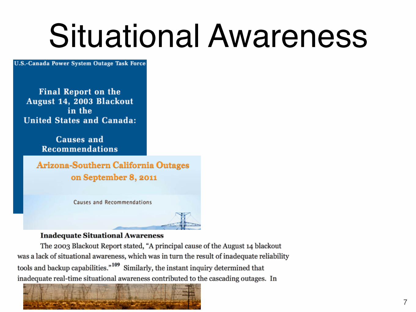
Situational Awareness
7

Situational Awareness
7

Situational Awareness
7
Situational Awareness
7

Situational Awareness
7

Situational Awareness
7

8
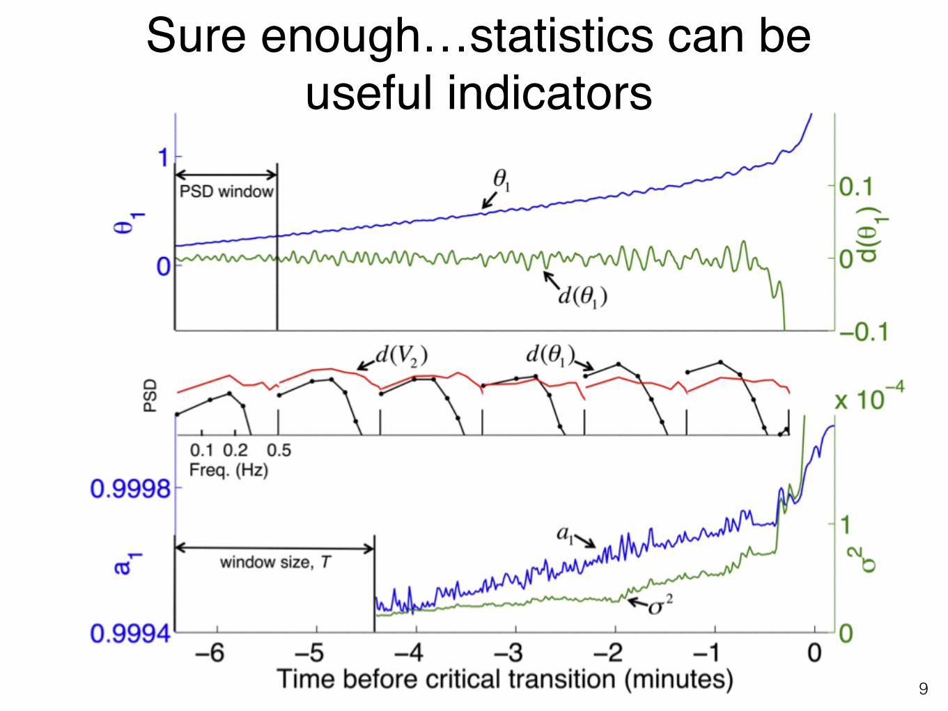
Sure enough…statistics can be useful indicators
9

Sure enough…statistics can be useful indicators
9

Sure enough…statistics can be useful indicators
9
Cotilla-Sanchez, Hines, Danforth, IEEE Trans Smart Grid, 2012. See also: DeMarco and Berge, IEEE Trans on Ckt & Sys, 1987.Dhople, Chen, DeVille, Domínguez-García, IEEE Trans on Ckt Sys, 2013Podolsky and Turitsyn, arXiv:1307.4318, Jul. 2013.Susuki and Mezic, IEEE Trans. Power Syst., 2012 (and others)
How can we find the useful* statistical early warning signs?
10
*Useful: A sign that shows up early enough that we might actually be able to do something about it, even if there is
measurement noise

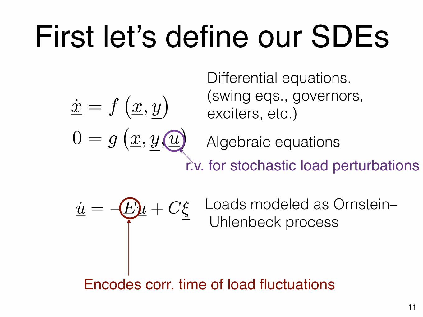
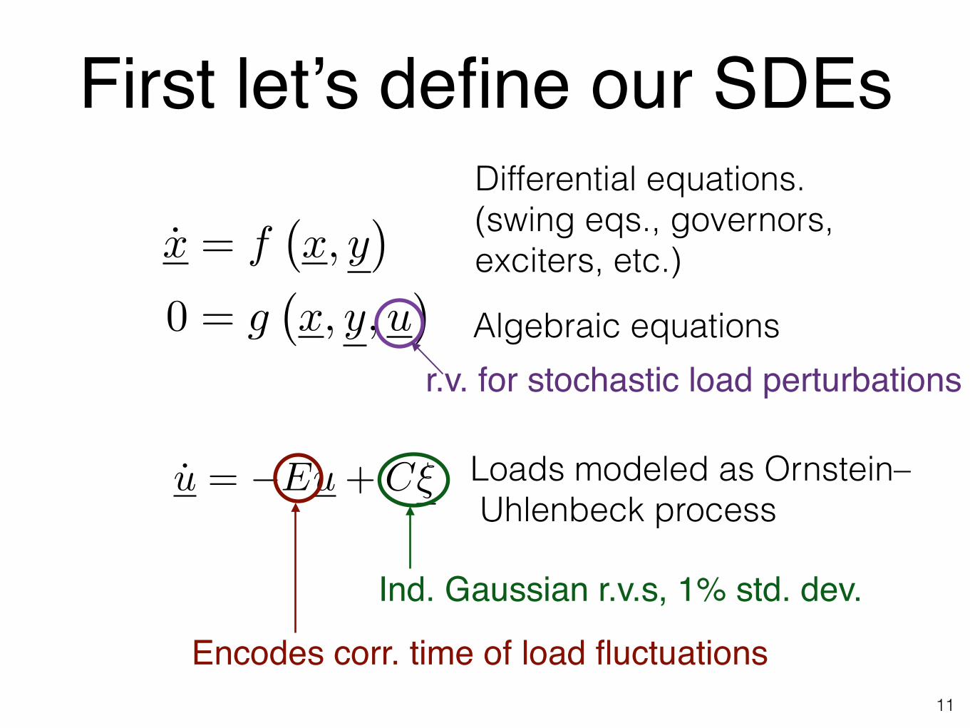
First let’s define our SDEs
11

First let’s define our SDEs
11
x = f
�x, y
�
0 = g
�x, y, u
�
Differential equations. (swing eqs., governors, exciters, etc.)
Algebraic equations

First let’s define our SDEs
11
x = f
�x, y
�
0 = g
�x, y, u
�
Differential equations. (swing eqs., governors, exciters, etc.)
Algebraic equationsr.v. for stochastic load perturbations

First let’s define our SDEs
11
x = f
�x, y
�
0 = g
�x, y, u
�
Differential equations. (swing eqs., governors, exciters, etc.)
Algebraic equationsr.v. for stochastic load perturbations
u = �Eu+ C⇠ Loads modeled as Ornstein– Uhlenbeck process
First let’s define our SDEs
11
x = f
�x, y
�
0 = g
�x, y, u
�
Differential equations. (swing eqs., governors, exciters, etc.)
Algebraic equationsr.v. for stochastic load perturbations
u = �Eu+ C⇠ Loads modeled as Ornstein– Uhlenbeck process
Encodes corr. time of load fluctuations
First let’s define our SDEs
11
x = f
�x, y
�
0 = g
�x, y, u
�
Differential equations. (swing eqs., governors, exciters, etc.)
Algebraic equationsr.v. for stochastic load perturbations
u = �Eu+ C⇠ Loads modeled as Ornstein– Uhlenbeck process
Encodes corr. time of load fluctuations
Ind. Gaussian r.v.s, 1% std. dev.
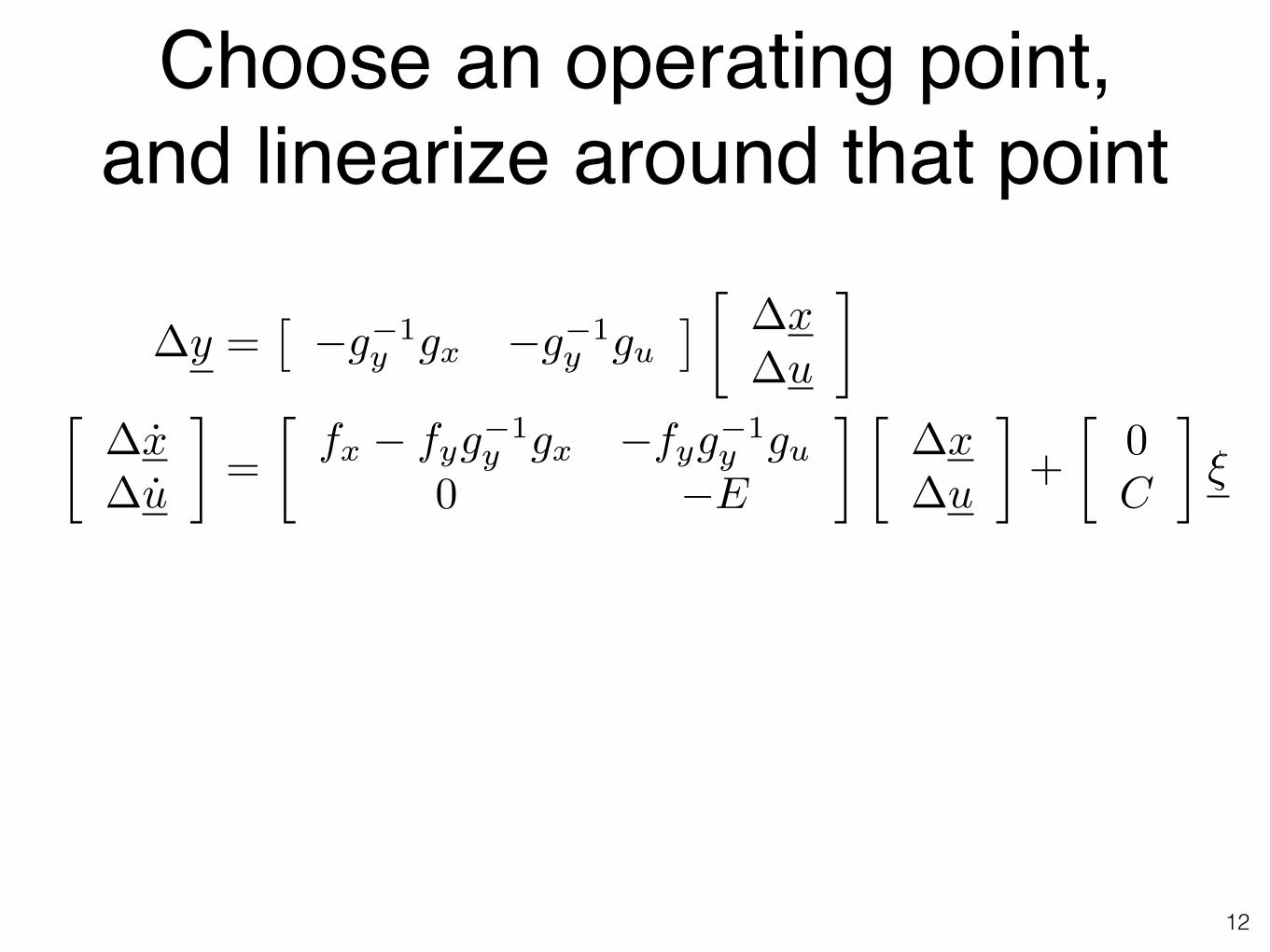
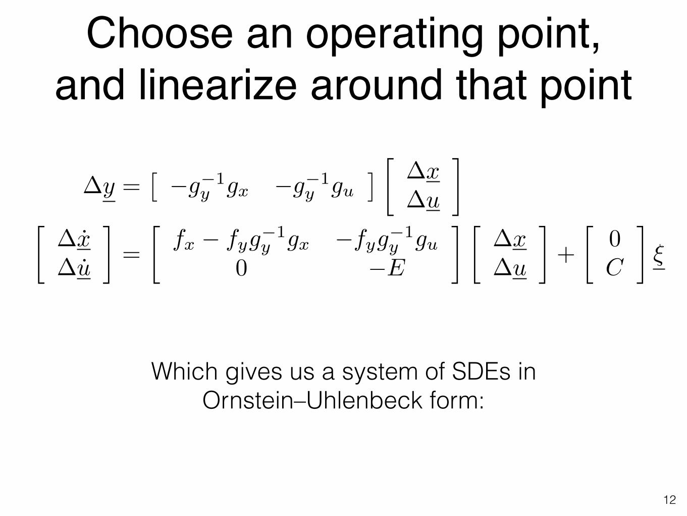
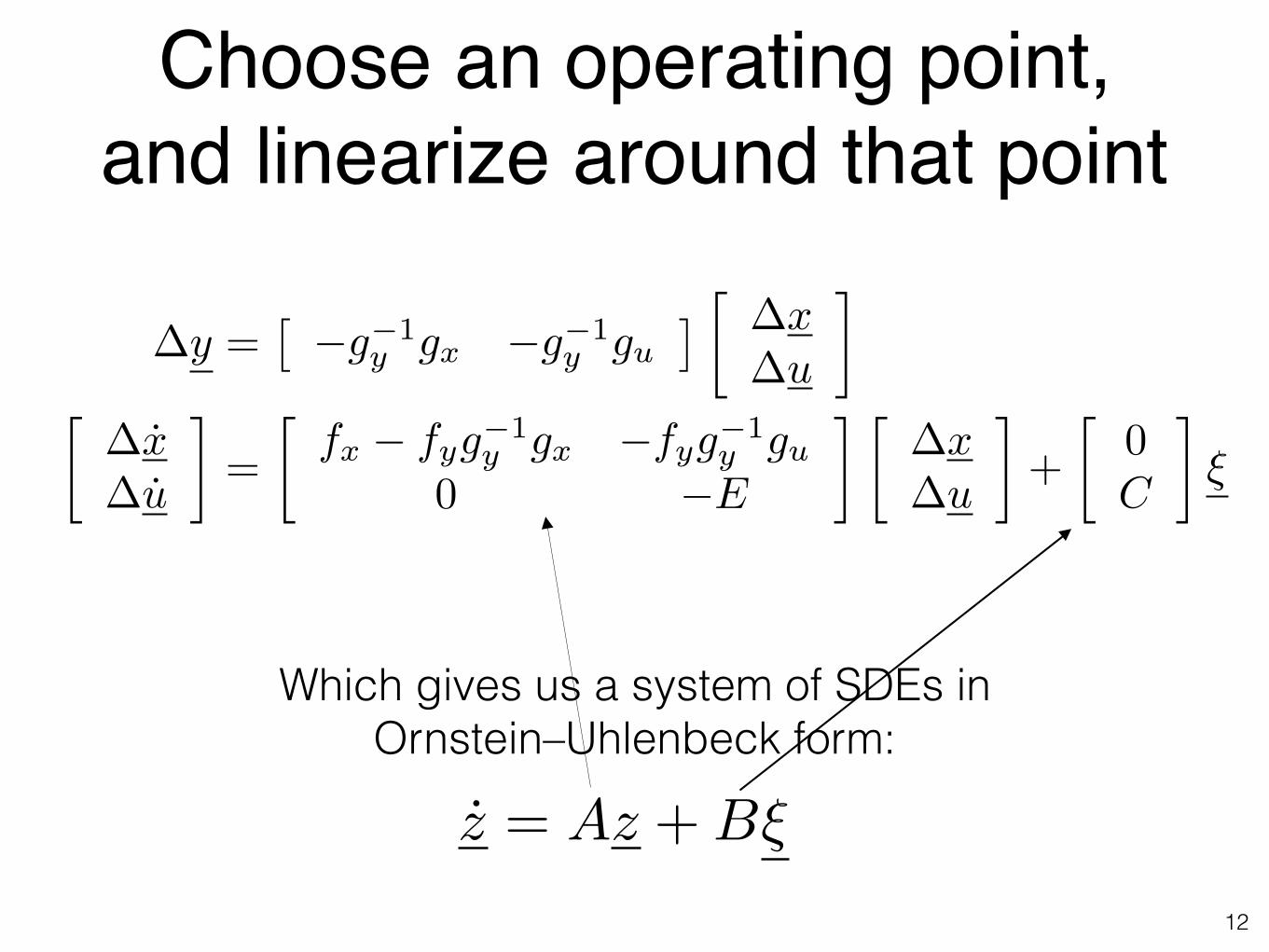
Choose an operating point, and linearize around that point
12
�y =⇥�g
�1y
g
x
�g
�1y
g
u
⇤ �x
�u
�
�x
�u
�=
f
x
� f
y
g
�1y
g
x
�f
y
g
�1y
g
u
0 �E
� �x
�u
�+
0C
�⇠

Choose an operating point, and linearize around that point
12
�y =⇥�g
�1y
g
x
�g
�1y
g
u
⇤ �x
�u
�
�x
�u
�=
f
x
� f
y
g
�1y
g
x
�f
y
g
�1y
g
u
0 �E
� �x
�u
�+
0C
�⇠
Jacobian matrix: df/dx

Choose an operating point, and linearize around that point
12
�y =⇥�g
�1y
g
x
�g
�1y
g
u
⇤ �x
�u
�
�x
�u
�=
f
x
� f
y
g
�1y
g
x
�f
y
g
�1y
g
u
0 �E
� �x
�u
�+
0C
�⇠
Choose an operating point, and linearize around that point
12
�y =⇥�g
�1y
g
x
�g
�1y
g
u
⇤ �x
�u
�
�x
�u
�=
f
x
� f
y
g
�1y
g
x
�f
y
g
�1y
g
u
0 �E
� �x
�u
�+
0C
�⇠
Which gives us a system of SDEs in Ornstein–Uhlenbeck form:

Choose an operating point, and linearize around that point
12
�y =⇥�g
�1y
g
x
�g
�1y
g
u
⇤ �x
�u
�
�x
�u
�=
f
x
� f
y
g
�1y
g
x
�f
y
g
�1y
g
u
0 �E
� �x
�u
�+
0C
�⇠
z = Az +B⇠
Which gives us a system of SDEs in Ornstein–Uhlenbeck form:
Choose an operating point, and linearize around that point
12
�y =⇥�g
�1y
g
x
�g
�1y
g
u
⇤ �x
�u
�
�x
�u
�=
f
x
� f
y
g
�1y
g
x
�f
y
g
�1y
g
u
0 �E
� �x
�u
�+
0C
�⇠
z = Az +B⇠
Which gives us a system of SDEs in Ornstein–Uhlenbeck form:

Now solve the SDEs
13

Now solve the SDEs
13
I’d like to tell you that we came up with new, elegant mathematics to solve. In reality…

Now solve the SDEs
13
I’d like to tell you that we came up with new, elegant mathematics to solve. In reality…

Now solve the SDEs
13
I’d like to tell you that we came up with new, elegant mathematics to solve. In reality…
A�z + �zAT= �BBT
E
⇥z (t) zT (s)
⇤= exp [�A|t� s|]�z

Now solve the SDEs
13
Lyapanov eq.
I’d like to tell you that we came up with new, elegant mathematics to solve. In reality…
A�z + �zAT= �BBT
E
⇥z (t) zT (s)
⇤= exp [�A|t� s|]�z

Now solve the SDEs
13
Lyapanov eq.
I’d like to tell you that we came up with new, elegant mathematics to solve. In reality…
And then reverse the Kron reduction to compute the variance and autocorrelation of voltage and current magnitudes.
A�z + �zAT= �BBT
E
⇥z (t) zT (s)
⇤= exp [�A|t� s|]�z

and choose a time delay for autocorrelation measurements
14

and choose a time delay for autocorrelation measurements
14

and choose a time delay for autocorrelation measurements
14

Check to make sure that the analytical and numerical line up
15

Check to make sure that the analytical and numerical line up
15

Check to make sure that the analytical and numerical line up
15

And add measurement noise
16

And add measurement noise
16
Which we can subsequently filter to largely regain our original signal,
with the interesting side-effect that some of the variance now appears as autocorrelation.
At key locations, we can see clear signs of instability in Autocorrelation and Variance
17
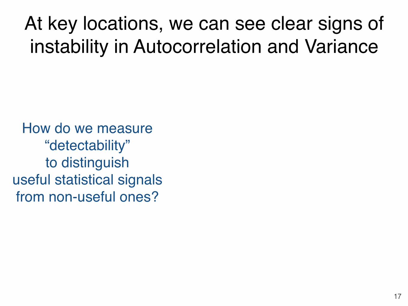
At key locations, we can see clear signs of instability in Autocorrelation and Variance
17
How do we measure“detectability”to distinguish
useful statistical signals from non-useful ones?
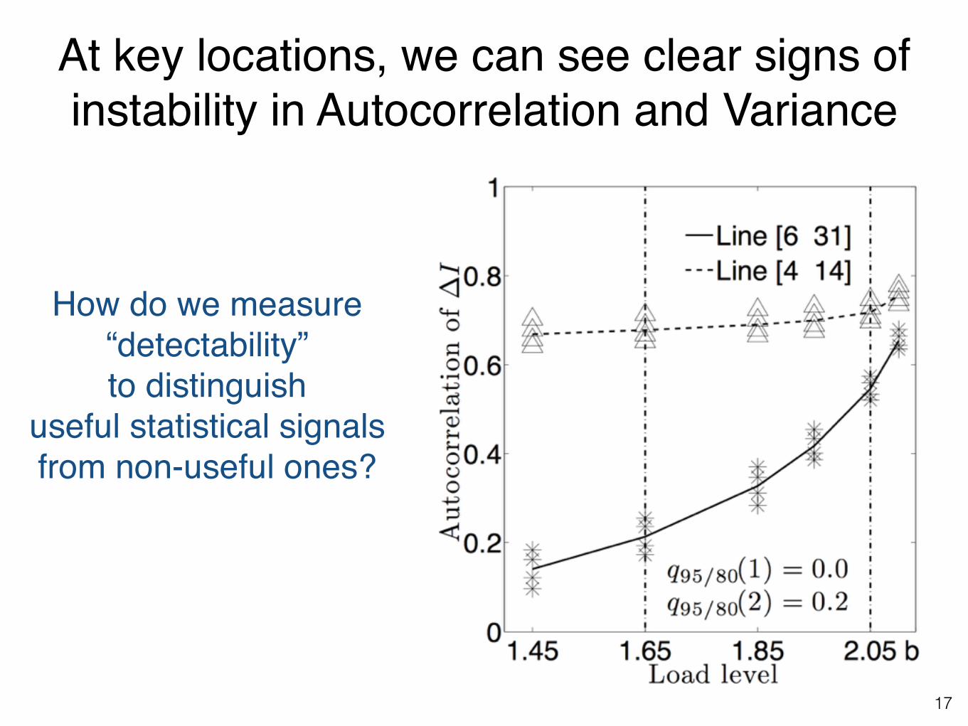
At key locations, we can see clear signs of instability in Autocorrelation and Variance
17
How do we measure“detectability”to distinguish
useful statistical signals from non-useful ones?
Which statistics provide useful (detectable)
early warning?
18
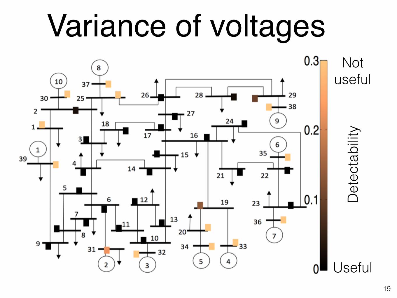
Variance of voltages
19
Not useful
Useful
Det
ecta
bilit
y
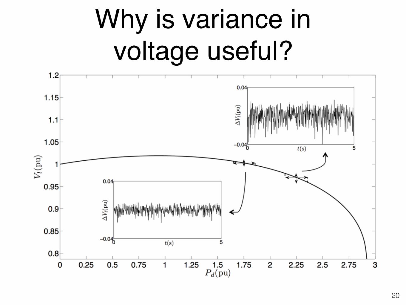
Why is variance in voltage useful?
20

Autocorrelation of currents
21
Not useful
Useful
Det
ecta
bilit
y
0
0.1
0.2
0.3

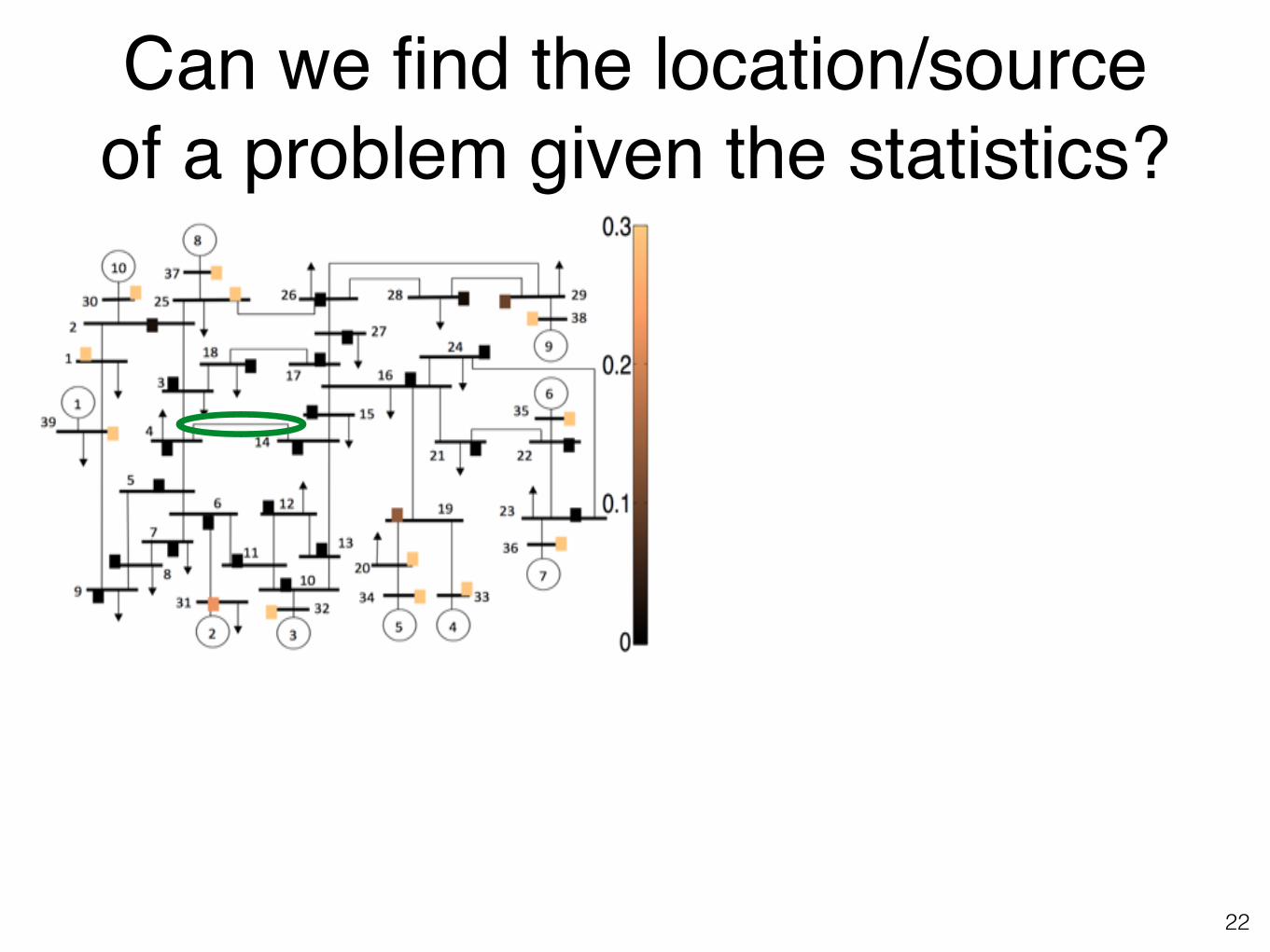
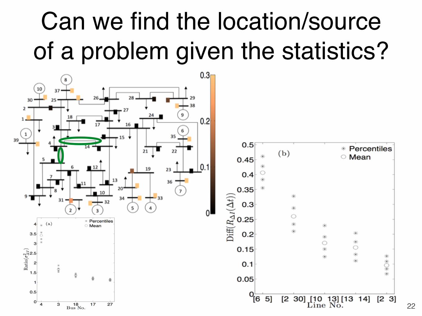
Can we find the location/source of a problem given the statistics?
22
Can we find the location/source of a problem given the statistics?
22

Can we find the location/source of a problem given the statistics?
22

Can we find the location/source of a problem given the statistics?
22

Can we find the location/source of a problem given the statistics?
22
Can we find the location/source of a problem given the statistics?
22

Can we find the location/source of a problem given the statistics?
22

Can we find the location/source of a problem given the statistics?
22

Can we find the location/source of a problem given the statistics?
22

Can we find the location/source of a problem given the statistics?
22

Can we find trends that would not show up in mean values?
23

Can we find trends that would not show up in mean values?
23

Can we find trends that would not show up in mean values?
23

Can we find trends that would not show up in mean values?
23

Can we find trends that would not show up in mean values?
23

Why not just monitor critical modes/eigenvalues?
24

Why not just monitor critical modes/eigenvalues?
24

Why not just monitor critical modes/eigenvalues?
24

In summary
25

In summary• Autocorrelation and variance are, sometimes, useful
indicators of proximity to instability.
25

In summary• Autocorrelation and variance are, sometimes, useful
indicators of proximity to instability.
• Variances of voltages near loads are consistently good indicators of proximity to voltage collapse, even when voltage magnitudes are not.
25

In summary• Autocorrelation and variance are, sometimes, useful
indicators of proximity to instability.
• Variances of voltages near loads are consistently good indicators of proximity to voltage collapse, even when voltage magnitudes are not.
• Autocorrelations of currents near generators (particularly smaller ones) are generally good indicators of system-wide stability issues (e.g., inter-area oscillations—Hopf bifurcation)
• Frequently, fluctuations can identify the locations of emerging problems in the network
25

Statistical Early Warning Signs of Instability in Synchrophasor Data
IEEE GMS/PES Synchrophasor Meeting October 12, 2016
Goodarz Ghanavati, Taras Lakoba, Paul Hines*
*To whom all blame is dueFunding gratefully acknowledged: NSF Awards ECCS-1254549, DGE-1144388, DOE Award DE-OE0000447 ,