1

Off-farm labour participation of farm couples. A bivariate random coefficients approach.

Hild-Marte Bjørnsen

marte.bjornsen@nibr.no

Norwegian Institute for Urban and Regional Research P.O.Box 44 Blindern, 0313 Oslo, Norway

Preliminary draft

Version of March 10th

Abstract When working with micro data one sometimes encounters situations involving qualitative choices rather than the continuous choices that are the traditional focus of empirical analysis. In this paper we investigate the probability of participating in off-farm work for Norwegian farm couples. We consider different ways of modelling the joint labour decisions of husband and wife through an agricultural household model that combines the agricultural production, consumption, and labour supply decisions in a single framework, and present the results of a bivariate random effects probit estimation. The model specification allows for dependence between the husband and wife’s decisions, and for heterogeneity between the households.

Keywords: Agricultural economics, time allocation, qualitative choice, bivariate probit,

simulated maximum likelihood, panel data,

JEL Classification: C33, C35, D11, D21, J22, J43

2

Introduction Farm household models have for more than two decades formed the theoretical framework for

empirical studies of farmers’ time allocation. The models are based on neoclassical

optimisation theory and treat the entire household as one unitary decision maker, without

considering differences in preferences amongst the household members. The households are

assumed to maximize utility as a function of total consumption and leisure, subject to

constraints on time, income and farm technology. The farm household model, in its most

general form, was first employed by Huffman (1980) and has since been developed to account

for specific problems such as zero farm work, hired labour, and joint decisions of husband

and wife. A considerable volume of empirical research on this issue has been produced on

American as well as European and Asian data. Kimhi (1994a, 1994b, 1996a, 1996b, 1996c,

1999, 2000, 2003) has given a large contribution in this field of research. Other major

contributors are Huffman (1980, 1989, 1991, 1998), Lass (1989, 1992, 1994) and Weersink

(1992, 1998, 2002). The majority of the analyses mentioned above are conducted on cross-

sectional data, but some studies, i.e. Weiss (1997), include off-farm work status in some

previous year as an explanatory variable in the cross-sectional setting. Corsi and Findeis

(2000) make use of a two-year panel to get univariate probit estimates of, respectively, the

operator and spouse’s off-farm labour participation, but they to not consider the

interdependencies between the decisions of operator and spouse. Their focus being state

dependence and heterogeneity in off-farm labour participation. Gould and Saupe (1989) have

done a joint estimation of the off-farm labour participation on two years separately, thus not

accounting for the panel data structure.

The neoclassical approach can be criticized for not giving a very adequate description

of human behaviour. Depending on the number of choice alternatives and the similarity of

these alternatives, it is not necessarily a simple task to rank the outcomes in a consistent and

well-defined manner. All individuals have their own preferences which may change over time

and under different conditions. Moreover, the assumption that everyone has full information

of all feasible choice alternatives is generally accepted as not a very realistic one. An

improvement of the neoclassical approach can be achieved by modelling the choice behaviour

as a probabilistic process. Although still a simplification, this will allow us to account for the

individual’s uncertainty by introducing randomness in the decision rule or in the utility

function. If we focus on the joint labour decisions of farm operator and spouse, game theory

may be an alternative way of modelling the time-allocation. If we assume that both operator

and spouse, at least partly, have concurrent interests, and that they are able to agree upon

maximising the household’s utility, this would make a cooperative game situation.

3

When modelling the joint decisions of two economic agents we also need to make

some assumptions about the dependence between their behaviour. There is one dichotomous

variable that needs explaining for each agent, namely whether to participate in off-farm work

or not, and we need to investigate the formal relationship between the operator and spouse’s

off-farm labour decisions. Particularly, we need to establish in what order decisions are being

made. Several models have been proposed to explain different kinds of joint strategies. One

way would be to assume that the operator (alternatively the spouse) makes the decision for the

entire household. In this case there is in fact only one decision maker and the modelling

problem equals a multinominal case with only one agent choosing between four alternative

work regimes. Another way of modelling the joint labour decisions could be a two-step

approach where we assume that the operator first decides his behaviour and that the spouse

subsequently makes her/his decisions conditionally on his/her choice. A third approach would

be to assume that both operator and spouse make their participation decisions conditional

upon the other one’s choice.

The aim of this paper is to make use of the panel data structure so as to be able to

include the dependence between the operator and spouse’s participation decisions as well as

the heterogeneity between households. We stick to the established theoretical framework and

apply the third approach to model dependencies between operator and spouse. The model is

then defined by four conditional distributions, and can be named conditional-conditional

(Gourieroux 2000) since both husband and wife’s behaviour is dependent on the spouse’s

course of action. In this case, the joint decisions can be modelled within a bivariate

framework where the dependence in behaviour is represented by the correlation between the

husband and wife’s participation rules. The participation probabilities of the two agents will

in this model include an identical vector of explanatory variables.

We have chosen to distinguish between farm operator and spouse instead of husband

and wife in this paper. As the operator is male in nearly all households in the sample, the

distinction is hardly recognisable. The majority of Norwegian farm units give full-time

employment to between 0.5 and 2 workers. Normally we find that the farm operator are

responsible for the daily running of the farm and that the spouse, other family members and

hired help contribute when and if needed. Most spouses in our sample work on the farm, but

there is a significant difference in the number of farm work hours supplied by operator and

spouse and consequently also in their opportunity to participate in off-farm work.

Models and estimation methods The theoretical foundation underlying the econometric model specifications bear resemblance

to models used by Huffman and Lange (1989), Gould and Saupe (1989), Lass and Gempesaw

4

(1992), and Weersink, Nicholson and Weerhewa (1997). The population of farm household

face the same choice set of alternative occupations. The decisions with respect to off-farm

employment are made jointly by operator and spouse and can result in four different and

mutually exclusive household off-farm work regimes:

1Y both operator and spouse participate in wage work: 0, 0O SM M> >

2Y only operator participates in wage work: 0, 0O SM M> =

3Y only spouse participates in wage work: 0, 0O SM M= >

4Y neither of them participates in wage work: 0, 0O SM M= =

where gM , g=O,S is the off-farm labour supply of the farm operator and spouse,

respectively.

The farm couple is assumed to maximise their joint utility subject to constraints on

time, income and farm production in a static framework. Utility can be derived from

purchased goods ( C ) and the farm couples’ leisure time ( ,O SL L ), and is affected by

variables such as human capital characteristics ( ,O SH H ), and other household and regional

(labour market) characteristics ( ZH , MZ ) that are considered exogenous to current

consumption decisions.

(1) ( ), , ; , , , , ' 0, , .gO S O S

H M LU U C L L H H Z Z U g O S= > =

The utility function is assumed to be ordinal and strictly concave. Operator and

spouse have separate time budgets and their total time endowment can be divided between

on-farm work (F), off-farm work (M), and leisure (L), all measured in hours. Both are

assumed to supply a strictly positive number of on-farm hours and to consume a positive

amount of leisure time. Time spent in the off-farm sector is non-negative for both operator

and spouse.

(4) , , 0, 0, ,g g g g g g gT F M L F L M g O S= + + > ≥ = .

Consumption is constrained by total net income. The household’s income is made up

of farm profits, PQ-RX (where P is output price, Q is output quantity, R is the input price

vector, and X is a vector of purchased farm inputs), net income from wage work (off-farm

work is paid at the wage rate W), and other household income net of taxes, interest payments

and losses (V).

(6) O O S SPQ W M W M V C RX+ + + = + .

5

The production technology of the farm represents the final constraint on the

household’s consumption possibilities. Farm output depends on the labour hours put down in

farm production, F, a vector of purchased input factors, X, human capital characteristics, H,

and farm specific characteristics, FZ (farm size, region etc.). Unlike wage work, farm work

is assumed to have diminishing marginal returns, i.e. the production function is assumed to be

strictly concave.

(5) ( ), , , , , , ' 0, '' 0O S O SFQ f F F X H H Z f f= > < .

The farm couple chooses levels of purchased goods and production inputs, leisure

time and labour supply in both occupations. The stock of human capital, regional, household

and farm characteristics, off-farm wage rates, input vector price, output price and other

income are exogenous to the maximisation problem.

Because of the non-binding constraints on off-farm work for both operator and

spouse, and on farm work for the spouse, the maximisation problem is non-linear. The off-

farm labour supply functions are determined by solving the Kuhn-Tucker conditions. An

interior solution exists if optimal allocation of time to leisure, on-farm, and off-farm work are

all nonzero for both operator and spouse.

Analytically, the reservation wage is derived from the utility maximising problem of

the farm household model and equals the marginal productivity of farm work, evaluated at

zero hours supplied of off-farm work. The reservation wage is unobservable, but defined as a

function of human capital, farm, household, and market characteristics.

(6) ' ( , , , , )gg O S

R F H MFW Pf w H H Z Z Z= = .

An individual i will participate in off–farm work at time t if the individual’s offered

wage rate ( gW ) exceeds the individual’s reservation wage ( RgW ).

(7) 0 if

, ,0 otherwise

g gg RW W

M g O S⎧> >

= =⎨=⎩

.

The decision rule holds for both operator and spouse, and whether or not the

individual has farm work as principal occupation. We are only able to observe the true wage

rate for the individuals’ who are actually working off the farm. Hence, the sample is censored

with respect to W.

The participation decision can then be represented by the following probabilities for

working off-farm for operator and spouse.

(8) Pr( ) Pr( ) Pr( ) Pr( )

Pr( ) Pr( ) Pr( ) Pr( )

O O O O S S O O S SR R R R R

S S S S O O S S O OR R R R R

O W W W W W W W W W W

S W W W W W W W W W W

= > = > > + > ≤

= > = > > + > ≤.

6

The bivariate probit model allows us to estimate separate equations for the operator

and spouse’s probabilities for participating in off-farm work. The two equations are estimated

jointly and the dependence between their decisions is represented through the correlation

coefficient ρ . If we let the households be indexed b 1,...,i N= , the time period in which the

households are observed be indexed by 1,...,t T= , and let g=O,S represent operator and

spouse, respectively, the choice variable for each individual is given by

(9) 1 if individual in houshold participates in off-farm work in year 0 otherwise

git

g i ty ⎧

= ⎨⎩

The observed variable gity is related to a latent variable *

gity that represents the

difference between the true wage rate and the reservation rate. *gity is defined as a linear

function of the explanatory variables.

(10) *

*

, ,

, ,Oit Oit O Oi Oit

Sit Sit S Si Sit

y x i t

y x i t

β α ε

β α ε

= + + ∀

= + + ∀

gitx is a row vector of covariates of the human capital, household, regional and farm

characteristics (see table 1). The contents of this vector follow from the model above. gβ is a

column vector of coefficients specific to operators and spouses, but constant over households

and time , giα is a random household effect, related to operator and spouse, representing

heterogeneity between households, and gitε is the true disturbance.

Within the random effects approach it is assumed that the individual-specific effects

( giα ) are stochastic, drawn from a known probability distribution, and independent of the

exogenous variables ( , g ,git O S=x ). We assume that the ,Oi Oiα α ’s are binormally

distributed with zero mean, standard deviation equal to ,O Sα ασ σ and correlation coefficient

θ . Likewise, we assume that the true error terms ( , )Oi Siε ε are symmetrical and standard

binormally distributed with zero mean, unit standard deviation ( 1)O Sε εσ σ= = , and

correlation coefficient ρ . There is no correlation between ( , )Oi Siα α and ( , )Oi Siε ε .

To formalise the implications of these assumptions, let

Oit Oi Oi

Sit Si Si

uu

α εα ε

= += +

.

We can then derive the following moments

7

( )

( )

( )

( )

2

2

2

0 , ,

( ) 1 , ,

,1

, , s t, ,1

,1

O

O S

O S

g

g

O S

O S

git

git

Oit Sit

git gis

Oit Sis

E u g O S

Var u g O S

Corr u u

Corr u u g O S

Corr u u

α

α α

α α

α

α

α α

α α

σ

σ σ θ ρσ σ

σ

σ

σ σ θσ σ

= =

= + =

+=

+

= ≠ =+

=+

.

The household specific effect gives rise to cross-period and cross-individual correlation

within the households.

The marginal density of Oitε and Sitε , and the joint density of ( ),Oit Sitε ε are

respectively,

( )21

212

uu eφ

π

−= , ( )

( )( )2 2 21 ( 2 ) / 1

22

1,2 1

u uv vu v e

ρ ρψ

π ρ

− − + −=

−,

and their CDFs are ( ) ( )x

x u duφ−∞

Φ = ∫ , ( ) ( ), ,x y

x y u v dudvψ−∞ −∞

Ψ = ∫ ∫ .

The response probabilities, conditional on ( ),Oi Siα α , associated with each of the four work

regimes, can be specified as follows

8

(11)

( ) ( )( )( )

( ) ( )( )

1

2

, Pr 1, 1 ,

Pr , ,

,

, Pr 1, 0 ,

Pr , ,

O Sit Oi Si it it Oi Si

Oit Oit O Oi Sit Sit S Si Oi Si

Oit O Oi Sit S Si

O Sit Oi Si it it Oi Si

Oit Oit O Oi Sit Sit S Si Oi Si

p y y

x x

x x

p y y

x x

x

α α α α

ε β α ε β α α α

β α β α

α α α α

ε β α ε β α α α

= = =

= > − − > − −

= Ψ + +

= = =

= > − − < − −

= Φ( ) ( )( ) ( )

( )( ) ( )

( ) ( )

3

4

,

, Pr 0, 1 ,

Pr , ,

,

, Pr 0, 0 ,

Pr

Oit O Oi Oit O Oi Sit S Si

O Sit Oi Si it it Oi Si

Oit Oit O Oi Sit Sit S Si Oi Si

Sit S Si Oit O Oi Sit S Si

O Sit Oi Si it it Oi Si

Oi

x x

p y y

x x

x x x

p y y

β α β α β α

α α α α

ε β α ε β α α α

β α β α β α

α α α α

ε

+ −Ψ + +

= = =

= < − − > − −

= Φ + −Ψ + +

= = =

= ( )( ) ( ) ( )

, ,

1 ,t Oit O Oi Sit Sit S Si Oi Si

Oit O Oi Sit S Si Oit O Oi Sit S Si

x x

x x x x

β α ε β α α α

β α β α β α β α

< − − < − −

= −Φ + −Φ + −Ψ + +

The likelihood function of the gity ’s, conditional on the 'itx s , but marginal with

respect to ( ),O Sα α , then becomes

( ) ( ) ( ) ( )1 4

1 41 1

, , , , , , , ,it it

O S

N Ty y

O S it Oi Si it Oi Si Oi Si Oi Sii t

L p p d dα αβ β σ σ θ ρ α α α α ψ α α α α∞ ∞

= =−∞ −∞

= ⋅⋅⋅∏ ∏∫ ∫

and the log likelihood function to be maximised with respect to Oβ , Sβ , Oσ , Sσ , ρ , andθ is:

( ) ( ) ( ) ( )1 4

1 41 1

ln , , , , , , , ,it it

O S

TNy y

O S it Oi Si it Oi Si Oi Si Oi Sii t

L p p d dα αβ β σ σ θ ρ α α α α ψ α α α α∞ ∞

= =−∞ −∞

= ⋅⋅⋅∑ ∏∫ ∫

Data The data is obtained from a yearly survey of Norwegian farm households (Account Results in

Agriculture and Forestry) collected by the Norwegian Agricultural Economics Research

Institute (NILF). The survey is one of the more comprehensive sources of farm statistics in

Norway, but has so far had little widespread use in applied research. The survey includes

approximately 1000 farm households representing different regions and principal productions

(grain, dairy, livestock etc.). Participation in the survey is voluntary but restricted to farmers

younger than the age of 67 (retirement age) and to farm households working at least 400 on-

farm hours on a yearly basis. Approximately 5 percent of the households are replaced each

year. The survey data is merged with official statistics on level of education from Statistics

Norway and with a regional classification standard.

9

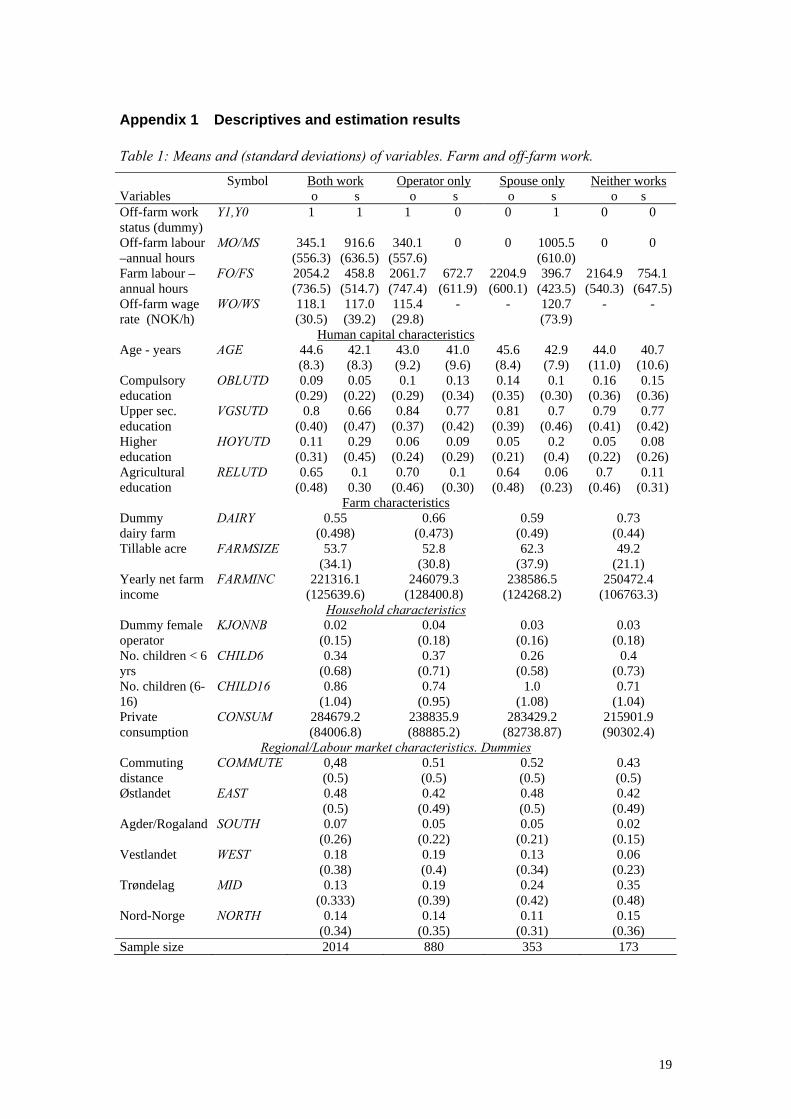
We have extracted a ten-year balanced panel (1991-2000) of 342 households of

married couples from the Account Results survey. The empirical definitions of the variables

and summary statistics are reported in table 1. We have divided the sample into the four

different work regimes and present the descriptives in means over the ten-year period for the

households in each category. We see that most households fall into the category where both

operator and spouse work off the farm. Only 173 of 3420 observations1 fall into the category

of traditional farming where neither works off thefarm. Farm and off-farm work are reported

in annual hours. The farm operators don’t, on average, supply many off-farm hours, but in all

four work regimes they work more than a standard labour year on the farm. Spouses take

more part in farm production when they don’t work off the farm. On average, the spouses

work less than operators, and they don’t supply a full man-labour year in either occupation.

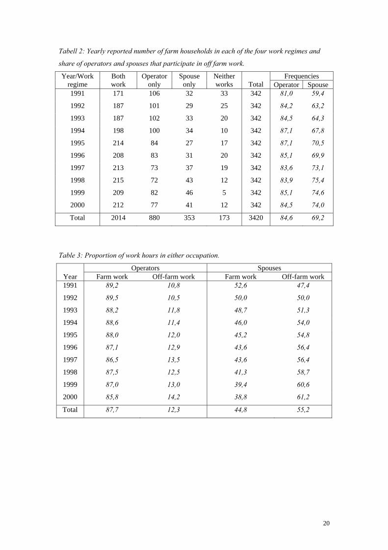
When we look at the summary statistics for one year at the time, we see that the number of

off-farm hours increases (19 pct for operators and 30 pct for spouses) while farm hours

decreases (to a lesser degree) from 1991 to 2000. In total, the spouses’ labour participation

increases by 13 percent and operators’ by one percent. On average, we find that

approximately 85 percent of all operators and 70 percent of all spouses participate in off-farm

work. The participation rates we find in this sample are high compared to other western

economies. In table 3, we look at the share of total working hours in both occupations for

each year. Operators spend the majority of their working hours on the farm, while spouses

divide their time more equally between farm and off-farm work. There is a marked trend

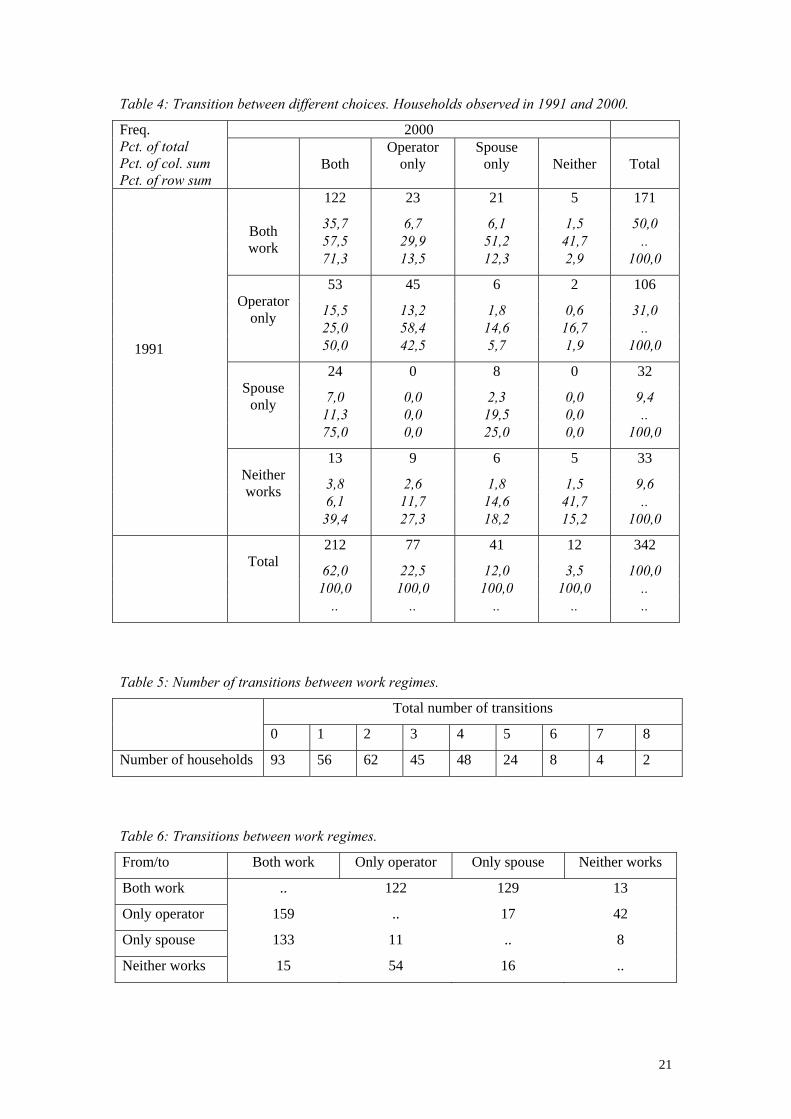
towards more hours spent in off-farm sector for both operators and spouses. Table 4 shows

transitions between the four work regimes from 1991 to 2000 and this table also bring

evidence of an increase in off-farm work.

The off-farm wage rate is in NOK per hour while net farm income, private

consumption, taxes, interest payment and income are reported in yearly figures. We have

scaled the economic variables into log-values in the estimations to avoid problems of too

different magnitudes of the variables. Farm income seems to be somewhat larger when

neither participates in off-farm work. We expect farm income to be correlated with farm size

and to have a negative effect on the probability of working off-farm.

Most individuals in sample have completed upper secondary schooling. Higher

education is more common among spouses that participate in off-farm work, while traditional

farm households where neither operator nor spouse works off-farm, have a higher proportion

1 We use observations instead of households because households may change work regime during the ten years of observation. In fact, we know for certain that it is not the same households that enters this category each year.

10

of compulsory schooling only. Approximately two thirds of the farm operators have

completed an education that in some respect is relevant to farming2.

The dummy for dairy includes all farms that produce dairy products. For some of

these farms dairy is the sole or principal farm output, while others combine dairy production

with other livestock farming (sheep, goats, swine, chicken), grain or forage. A large

proportion of the farms in the sample falls within this dairy farm definition, and the highest

percentage is found among households where neither works off the farm. Since dairy farms

are relatively labour intensive, we would assume a negative effect on off-farm work,

particularly for the farm operators.

Farm size measured in acres ranges from 9 to 229 with average farm size equal to 54

acres. When we split the statistics on single years we see that average farm size increases each

year from 49 acres in 1991, to 60 acres 2000. The increase in farm size can be explained by a

decline in the total number of operative farms with former farmers putting land out for sale or

hire. In 1999 nearly one third of all cultivated land was leased (Ssb 2002). Most farms are run

by male operators. We see that only 2-4 percent of the operators are female. The largest

proportion of female operators is found in the category where only operators work off the

farm, but the proportion does not seem to change much with work regime.

On average, the households in the sample do not have many small children and the

proportion is decreasing over the years. This is not surprising considering the average age of

operator and spouse. It seems that more of the households where neither works off the farm

have small children. In the literature, it is generally assumed that preschool-aged children

decrease the probability of off-farm work, particularly for women. More households seem to

have children in the age group 6 to 16 years old and the highest average number of children is

reported for households where the spouse works off the farm.

The location variable is a dummy representing distance to nearest city of a certain

size. This variable equals one if the commuting distance to a city with at least 15 000

inhabitants is less than one hour. Approximately half the farms have a central or fairly central

localisation. The effect of centrality on off-farm participation is not unambiguous. When a

farm has a central location it will probably be easier for the farm couple to find suitable off-

farm labour within commuting distance. Seen isolated, this is assumed to increase the

participation probability. We find in the descriptives that the category where neither works

off-farm has a relatively low proportion of centrally localised farms. On the other hand, we

know that the more centrally located farms are usually also the largest farms. The more labour

input is required on the farm, and the higher the farm income, the lower is the expected

2 The dummy for relevant education includes agriculture and forestry, veterinary, and some engineering and mechanics. We include education both on secondary and higher levels in this dummy.

11

probability of participating in off-farm work. A priori, the effect of centrality on off-farm

participation is thus ambiguous.

When we look at the regional spread, we find that most of the farms in the sample are

located in the south-eastern part of Norway, while Agder and Rogaland (southern region) is

more sparsely represented. If we distinguish between the four work regimes we see that a

rather large proportion of the farms where neither works off-farm is located in Trøndelag,

with correspondingly fewer farms in this category in southern and western parts of the

country.

Empirical results The results are computed using LIMDEP Verson 8.0, econometric software. The random

effects bivariate probit model is computed within the random parameters (rpm) framework as

the simpler random effects model doesn’t support panel data. The rpm framework allows for

individual heterogeneity in the beta parameters as well as in the household specific

parameter iα , but this will not be considered in the following. Model description and

commands for the rpm model and the bivariate probit model can be found in the LIMDEP 8.0

manual, chapters E14 and E16, respectively. In the ML estimation, we have set the starting

values to equal 1O Sα ασ σ= = and 0O Sβ β= = . Other staring values did not give higher

value of the likelihood function. Likelihood ratio tests for restrictions on the beta parameters

did not support rejection of any explanatory variables. In the simulations, the number of

random draws from the distribution is set to 200 in order to obtain convergence, but we have

implied the Halton sequence to reduce the number of draws and consequently, the

computation time. LIMDEP computes the bivariate normal probabilities using a 15 point

Gauss-Laguerre quadrature, for details see the manual page R5-22.

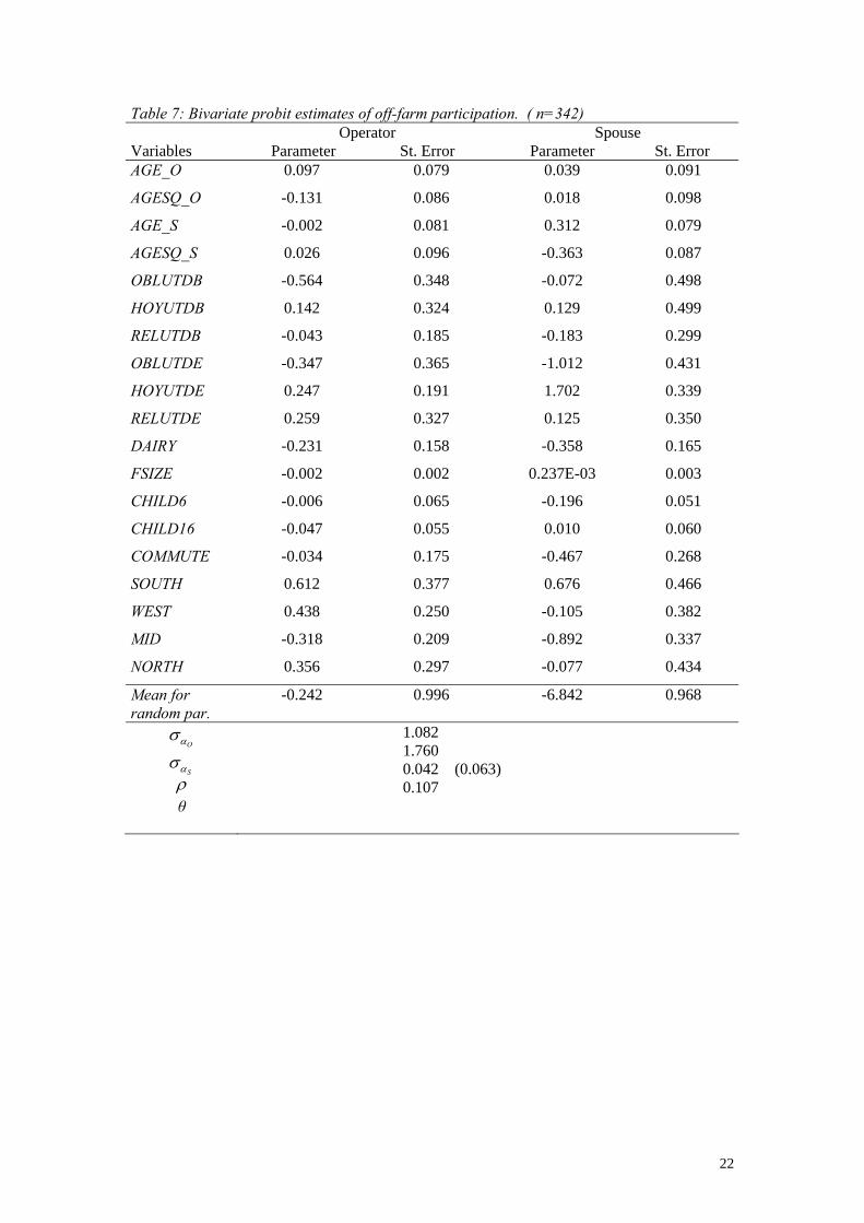
The bivariate probit estimates for operator and spouse are presented in table 7. A

Wald test does not reject the hypothesis that 0ρ = . This is an indication that we don’t gain

anything in way of efficient estimation by applying a bivariate specification instead of

separate probit estimations for operator and spouse.

There seems to be much latent heterogeneity in the model because the estimated

variance of the random household effects is rather large. We see that the correlation of the

household effects between operator and spouse, θ , is also close to zero. When we reduce the

number of human capital characteristics, θ increases.

Not many of the parameter estimates for the operators are significantly different from

zero: For spouses, the number of significant estimates are higher. All models include the same

12

vector of explanatory variables which is identical for operator and spouse. The only

transformed variable in the estimations is the age variable that also appears in quadratic form.

Marginal effects

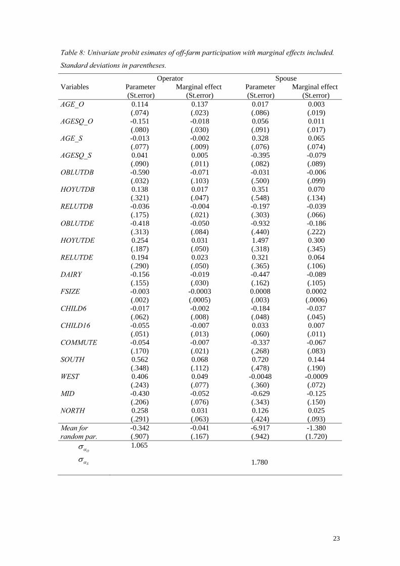
We have found no evidence to support the use of a bivariate model. To simplify the

calculations, we have thus derived the marginal effects from univariate models for operator

and spouse, respectively. The univariate estimation results and the marginal effects are

reported in table 8.

We distinguish between four groups of explanatory variables in the model: (i) human

capital characteristics, (ii) farm characteristics, (iii) household characteristics, and (iv)

regional/labour market characteristics. If we look at the individual characteristics, we see that

own age show a quadratic age pattern on off-farm participation. The probability of

participating in off-farm work increases with age, peaks at the age of 44 for operators and 42

for spouses, when it starts to decline. Own age effects are significant for spouses, but not for

operators. Cross age effects are not significantly different from zero. A priori, age can be

thought of as having an ambiguous effect on off-farm participation as it affects both farm

labour productivity and the market wage. There seems to be a positive relationship between

level of education and off-farm work participation for both operator and spouse. When you

only have finished compulsory education you may find it more difficult to find a satisfactory

job, and you may get higher returns by spending your time in farm production. We see that

only having completed compulsory education reduces the probability of off-farm participation

by 7 percent for operators and 3 percent for spouses compared to if they had completed

secondary schooling. Higher education increases your off-farm work possibilities, and may

even put you in a position where you, to a greater extent, can have flexible hours, thus making

it simpler to combine with farm production. Higher education has a significant and strong

effect on the spouses’ participation probability, increasing it by as much as 30 percent. For

operators, the probability only increases by less than 2 percent which is less that the 3 percent

cross effect of spouses’ higher schooling. The cross effect is positive (3.5 pct) and significant

for the spouses. Operators’ agricultural education is, quite as expected, negatively related to

off-farm participation, though not significantly so and only by 0.4 percent. The assumption is

that the more specialised you are, the higher is the expected productivity in farm production,

and the higher wage compensation you would ask for in order to participate in off-farm work.

When farm operators have agricultural schooling, this also reduces the probability of the

spouse’s off-farm participation. More surprisingly, we find that the spouse’s agricultural

education is positively related to both own off-farm participation and that of operators. This

result is not intuitive, but one explanation may be the broad definition of agricultural

education we apply. Within the definition we include, among other things, veterinary college,

13

while veterinary will be defined as off-farm work. The increase in the operator’s off-farm

participation may be induced by the spouse’s better ability to work on the farm.

The variables representing farm characteristics have a negative effect on off-farm

work participation. Dairy production is rather labour intensive and the milk cattle demand

attendance several times per day, which can make dairy farming difficult to combine with

other occupations. Still, we find that dairy farming have a greater effect on the spouse’s

participation probability than that of the operator, 9 versus 2 percent, respectively. Again, it

is only the coefficient estimate for the spouse that is significantly different from zero. A

priori, we would assume farm size to affect off-farm work in a negative manner, but this need

not be the case. The largest farms are often all grain producers, located in wide and flat

landscape, and thus highly productive. Grain production is generally accepted as being the

easiest production type to combine with other employments, partly because they are labour

intensive only in short time intervals of the year, It is highly mechanised, one can more easily

get hired help, and these farm are often rather centrally located with respect to commuting

distance to the largest cities. In the estimation results, we find that an increase in farm size has

practically no effect on the participation probabilities, but that the sign of the parameter is

negative for operators while positive for spouses.

Preschool-aged children reduce the probability of taking on off-farm work for both

operator and spouse. The spouses, of whom most are female, have a significant four percent

decrease in their participation probability for each child younger than six. Older children, in

the age group 6-16, reduce the operator’s participation probability, but increase that of the

spouse. Neither of these parameters are significantly different from zero. The increased

participation probability of the spouses may be explained by a wish to re-enter the labour

market after a period of staying at home with small children.

The commuting dummy, which indicates whether the farm is centrally located, have a

negative effect on off-farm participation. This means that living near a larger town or city

reduces the participation probability. This is a rather surprising result and estimates are not

stistically significant. As already mentioned, this negative effect may be explained by the fact

that the more centrally located farms are usually also both the larger and the more profitable

ones. Being located in the southern region, Agder and Rogaland, increases the probability of

participating in off-farm work by 7 and 14 percent respectively for both operator and spouse.

A northern location equivalently raised probability by 3 percent for both operator and spouse.

Living in Trøndelag (MID) reduces the participation probabilties. This region houses a large

proportion of the major grain producers. Being located in the western region, Vestlandet, has

a positive effect (5 pct. increase) on the operators’ participation decision, but a negative effect

on that of the spouses. These regional effects are compared to living in the more densely

14

populated eastern region, Østlandet. Except for the MID parameter for operators, neither of

these parameters is significantly different from zero.

Conclusions, comments and further challenges The aim of this paper has been to make use of the panel data structure to account for the

dependence between the farm operator and the spouse’s decisions on off-farm labour

participation. We have kept within the established theoretical framework of a household

production model that was first applied by Huffman (1980). The main extensions we have

made compared with earlier studies, is to include household specific effects and to test for

correlation between operator and spouse by conducting the analysis on a fairly large panel

data set. We have not found evidence to support the hypothesis that joint participation

decisions within a bivariate modelling framework is more efficient than of separate decision

making. The correlation coefficient between the operator and spouse’s participation

probabilities was not significantly different from zero.

The estimation results of both the bivariate and the univariate probit models are in

accordance with the results of similar studies3, primarily conducted on American and

Canadian data, and with our a priori assumptions of the causal relationship between

participation decisions and the explanatory model. Participation was found to show a concave

life cycle pattern, first increasing and then decreasing with age. Higher education increases

the probability of working off the farm, while lack of education decreases the participation

probability. The number of children, particularly preschool-aged children, decreases the

probability of participating in off-farm work, most markedly for the spouses. Labour intensive

dairy production was found to decrease the participation probability, just as we expected, but

farm size was found to have a more ambiguous effect on participation. The marginal effect of

farm size was close to zero for both operator and spouse, though negative for the operator and

positive for the spouse. We have mentioned some possible interpretations of this result in the

text above.

The off-farm participation rate is very high in Norwegian farm households compared

to other western economies. Moreover, the participation rate has increased on a yearly basis

throughout the observed decade, reaching 85 percent for operators and 74 percent for spouses

in 2000. This change towards more time being spent off the farm seems to continue despite

the fact that most farmers prefer full time to part time farming (Ssb 1998). There has been a

simultaneous increase in the exit rate from farming, partly induced by the younger generation

being less inclined to taking over the family farm. The agricultural sector is undergoing major

structural changes forced on by, among other things, the liberalisation of trade with building

3 For references, see page 4, or the literature list below.

15

down of tariffs and quotas, and with subsequently lower output prices, and by governmentally

induced output quotas. In Norway, both natural given factors such as climate and topography,

and social conditions such as a tradition for small family farms and strong governmental

regulations, contribute in making this process hard on the traditional full time farmer. Even

so, part time farming is not a new phenomenon. There are long traditions for combining

farming with other occupations, such as i.e. coastal fishing and small scale craft industries.

The golden era for the full time farmer found place in the post war period towards the 1980s

when the pay settlement for the agricultural sector followed the wage growth in the

manufacturing industries, but these policy objectives are no longer as stringent as they used to

be.

We have not been able to consider all aspects outlined in the introduction. The scope

of the essay has mainly been to model the joint decisions of operator and spouse to see

whether they are strongly correlated or not. We have mentioned that the established

theoretical model framework has its deficiencies. We will look further into that aspect in a

forthcoming essay that include randomness in the decision making process. This paper will

include both the discrete choice of entering the off-farm labour market, and the continuous

choice of determining labour supply both on the farm and off the farm. Another problem that

we have not treated empirically here is a comparison between different ways of modelling the

dependencies between the farm couple off-farm participation decisions. The data does not

lend itself easily to the multinominal model because they do not include variables that are

specific each of to the four work regimes.

16

Literature Anderson, S.P., A. De Palma, and J.-F. Thisse. (1992): Discrete Chioce Theory of Product

Differentiation. Cambridge: MIT Press.

Corsi, A. and J.L. Findeis (2000): “True state dependence and heterogeneity in off-farm

labour participation.” European Review of Agricultural Economics n. 2, 2000, 127-151.

Findeis, J. and D. Lass (1994): “Labor Decisions by Agricultural Households:

Interrelationships between Off-Farm Labor Supply and Hired Labor Demand.” Working

paper #94-08. Population Research Institute, The Pennsylvania State University, 1994.

Gould, B.W, and W.E. Saupe. (1989): “Off farm labor market entry and exit.” Amer. J. Agr.

Econ. 71, 960-967.

Gourieroux, C. (2000): Econometrics of Qualitative Dependent Variables. Cambridge

University Press.

Greene, W.H. (1997): Econometric Analysis. Prentice-Hall, New Jersey.

Hanemann, W.M. (1984): “Discrete/Continuous Models of Consumer Demand.”

Econometrica Vol. 52, Issue 3, 541-562.

Heckman, J.J. and E. Leamer (eds.):

Hsiao, C. (1995): Logit and Probit models in The Econometrics of Panel Data. A Handbook

of the Theory with Applications., ed. by Mátyás, L. and P. Sevestre, pp.410-428, Dordrecht:

Kluwer Academic Publishers.

Kimhi, A. (1994a): “Participation of Farm Owners in Farm and/or Off-Farm Work Including

the Option of Full-Time Off-Farm Work.” Journal of Agricultural Economics 45, 1994, 232-

239.

Kimhi, A. (1994b): “Quasi-Maximum Likelihood Estimation of Multivariate Probit Models:

Farm Couples’ Labor Participation.” American Journal of Agricultural Economics 76, 1994,

828-835.

Kimhi, A. (1996a): “Farmers’ Time Allocation between Farm Work and Off-Farm Work and

the Importance of Unobserved Group Effects: Evidence from Israeli Cooperatives.”

Agricultural Economics 14, 1996, 135-142.

Kimhi, A. and M.-j. Lee (1996b): “Joint Farm and Off-Farm Work Decisions of Farm

Couples: Estimating Structural Simultaneous Equations with Ordered Categorical Dependent

Variables.” American Journal of Agricultural Economics 78, 1996, 687-698.

Kimhi, A. (1996c): “Off-Farm Work Participation of Israeli Farm Couples.” Canadian

Journal of Agricultural Economics 44, 1996, 481-490.

Kimhi, A. and R. Bollman (1999): “Family Farm Dynamics in Canada and Israel. The case of

Farm Exits.” Agricultural Economics 21, 1999, 69-79.

Kimhi, A. (2000): “Is Part-Time Farming Really a Step in the Way Out of Agriculture?”

American Journal of Agricultural Economics 82, 2000, 38-48.

17

Kimhi, A. (2003): “Family Composition and Off-Farm Participation Decisions in Israeli Farm

Households.” American Journal of Agricultural Economics .

Huffman, W.E. (1980): “Farm and Off-Farm Work Decisions. The Role of Human Capital.”

Review of Economics and Statistics 62, 1980, 14-23.

Huffman, W.E., and M.D. Lange. (1989): “Off-farm work decisions of husbands and wives:

joint decision making.” Review of Economics and Statistics. 71, 471-480.

Huffman, W.E., and H. El-Osta. (1998): “Off-Farm Work Participation, Off-Farm Labor

Supply and On-Farm Labor Demand of U.S. Farm Operators.” American Journal of

Agricultural Economics. 80, 1180-.

Lass, D.A., J. Findeis and M.C. Hallberg (1989): “Off-Farm Employment Decisions by

Massachusetts Farm Households.” Northeastern.Journal of Agricultural and Resource

Economics. 18, 1989, 149-159411.

Lass, D.A., and C.M. Gempesaw II. (1992): “The Supply of Off-Farm Labor: A Random

Coefficient Approach.” Amer. J. Agr. Econ. 74, 400-411.

Maddala, G.S. (1983): Limited-dependent and qualitative variables in econometrics.

Cambridge University Press.

Manski, C. F. (1977): ”The Structure of Random Utility Models.” Theory and Decision 8:

229-254.

Manski, C. F. (1987): ”Semiparametric Analysis of Random Effects Linear Models from

Binary Panel Data.” Econometrica, 59, pp. 357-362.

Neyman, J. and E.L. Scott (1948): “Consistent estimates Based on Partially Consistent

Observatins.” Econometrica 16:1-32.

Phimister, E., E. Vera-Toscano and A. Weersink (2002): “Female Participation and Labor

Market Attachment in Rural Canada.” American Journal of Agricultural Economics 40, 2002,

210-221.

Statistisk sentralbyrå (1998): Levekår i landbruket. Rapport 98/25. Statistisk sentralbyrå.

Oslo-Kongsvinger.

Statistisk sentralbyrå (2002): Jordbrukstellinga 1999. NOS C760. Oslo-Kongsvinger.

Tokle, J.G. and W.E. Huffman (1991): “Local Economic Conditions and Wage Labor

Decisions of Farm and Rural Nonfarm Couples.” American Journal of Agricultural

Economics. 73, 652-670.

Tversky, A. (1972): “Elimination by Aspects: A Theory of Choice.” Psychological Rewiev

79: 281-299.

Weersink, A. (1992): “Off-Farm Labour Decisions by Ontario Swine Producers.” Canadian

Journal of Agricultural Economic 40, 1992, 235-252.

Weersink, A., Nicholson, C., and J. Weerhewa. (1998): “Multiple job holdings among dairy

farm families in New York and Ontario.” Agricultural Economics. 18, 127-143.

18

Weiss, C. (1997): “Do they come back again? The symmetry and reversibility of off-farm

employment.” European Review of Agricultural Economics 24, 1997, 65-84.

19

Appendix 1 Descriptives and estimation results Table 1: Means and (standard deviations) of variables. Farm and off-farm work.

Variables

Symbol Both work o s

Operator only o s

Spouse only o s

Neither works o s

Off-farm work status (dummy)

Y1,Y0 1 1 1 0 0 1 0 0

Off-farm labour –annual hours

MO/MS 345.1 (556.3)

916.6 (636.5)

340.1 (557.6)

0 0 1005.5 (610.0)

0 0

Farm labour –annual hours

FO/FS 2054.2(736.5)

458.8 (514.7)

2061.7(747.4)

672.7 (611.9)

2204.9(600.1)

396.7 (423.5)

2164.9 (540.3)

754.1 (647.5)

Off-farm wage rate (NOK/h)

WO/WS 118.1 (30.5)

117.0 (39.2)

115.4 (29.8)

- - 120.7 (73.9)

- -

Human capital characteristics Age - years AGE 44.6

(8.3) 42.1 (8.3)

43.0 (9.2)

41.0 (9.6)

45.6 (8.4)

42.9 (7.9)

44.0 (11.0)

40.7 (10.6)

Compulsory education

OBLUTD 0.09 (0.29)

0.05 (0.22)

0.1 (0.29)

0.13 (0.34)

0.14 (0.35)

0.1 (0.30)

0.16 (0.36)

0.15 (0.36)

Upper sec. education

VGSUTD 0.8 (0.40)

0.66 (0.47)

0.84 (0.37)

0.77 (0.42)

0.81 (0.39)

0.7 (0.46)

0.79 (0.41)

0.77 (0.42)

Higher education

HOYUTD 0.11 (0.31)

0.29 (0.45)

0.06 (0.24)

0.09 (0.29)

0.05 (0.21)

0.2 (0.4)

0.05 (0.22)

0.08 (0.26)

Agricultural education

RELUTD 0.65 (0.48)

0.1 0.30

0.70 (0.46)

0.1 (0.30)

0.64 (0.48)

0.06 (0.23)

0.7 (0.46)

0.11 (0.31)

Farm characteristics Dummy dairy farm

DAIRY 0.55 (0.498)

0.66 (0.473)

0.59 (0.49)

0.73 (0.44)

Tillable acre FARMSIZE 53.7 (34.1)

52.8 (30.8)

62.3 (37.9)

49.2 (21.1)

Yearly net farm income

FARMINC 221316.1 (125639.6)

246079.3 (128400.8)

238586.5 (124268.2)

250472.4 (106763.3)

Household characteristics Dummy female operator

KJONNB 0.02 (0.15)

0.04 (0.18)

0.03 (0.16)

0.03 (0.18)

No. children < 6 yrs

CHILD6 0.34 (0.68)

0.37 (0.71)

0.26 (0.58)

0.4 (0.73)

No. children (6-16)

CHILD16 0.86 (1.04)

0.74 (0.95)

1.0 (1.08)

0.71 (1.04)

Private consumption

CONSUM 284679.2 (84006.8)

238835.9 (88885.2)

283429.2 (82738.87)

215901.9 (90302.4)

Regional/Labour market characteristics. Dummies Commuting distance

COMMUTE 0,48 (0.5)

0.51 (0.5)

0.52 (0.5)

0.43 (0.5)

Østlandet EAST 0.48 (0.5)

0.42 (0.49)

0.48 (0.5)

0.42 (0.49)

Agder/Rogaland SOUTH 0.07 (0.26)

0.05 (0.22)

0.05 (0.21)

0.02 (0.15)

Vestlandet WEST 0.18 (0.38)

0.19 (0.4)

0.13 (0.34)

0.06 (0.23)

Trøndelag MID 0.13 (0.333)

0.19 (0.39)

0.24 (0.42)

0.35 (0.48)

Nord-Norge NORTH 0.14 (0.34)

0.14 (0.35)

0.11 (0.31)

0.15 (0.36)

Sample size 2014 880 353 173

20

Tabell 2: Yearly reported number of farm households in each of the four work regimes and

share of operators and spouses that participate in off farm work.

Frequencies Year/Work regime

Both work

Operator only

Spouse only

Neither works

Total Operator Spouse

1991 171 106 32 33 342 81,0 59,4

1992 187 101 29 25 342 84,2 63,2

1993 187 102 33 20 342 84,5 64,3

1994 198 100 34 10 342 87,1 67,8

1995 214 84 27 17 342 87,1 70,5

1996 208 83 31 20 342 85,1 69,9

1997 213 73 37 19 342 83,6 73,1

1998 215 72 43 12 342 83,9 75,4

1999 209 82 46 5 342 85,1 74,6

2000 212 77 41 12 342 84,5 74,0

Total 2014 880 353 173 3420 84,6 69,2

Table 3: Proportion of work hours in either occupation.

Operators Spouses Year Farm work Off-farm work Farm work Off-farm work 1991 89,2 10,8 52,6 47,4

1992 89,5 10,5 50,0 50,0

1993 88,2 11,8 48,7 51,3

1994 88,6 11,4 46,0 54,0

1995 88,0 12,0 45,2 54,8

1996 87,1 12,9 43,6 56,4

1997 86,5 13,5 43,6 56,4

1998 87,5 12,5 41,3 58,7

1999 87,0 13,0 39,4 60,6

2000 85,8 14,2 38,8 61,2

Total 87,7 12,3 44,8 55,2

21

Table 4: Transition between different choices. Households observed in 1991 and 2000.

2000 Freq. Pct. of total Pct. of col. sum Pct. of row sum

Both

Operator only

Spouse only

Neither

Total

122 23 21 5 171

35,7 6,7 6,1 1,5 50,0 57,5 29,9 51,2 41,7 ..

Both work

71,3 13,5 12,3 2,9 100,0

53 45 6 2 106

15,5 13,2 1,8 0,6 31,0 25,0 58,4 14,6 16,7 ..

Operator

only

50,0 42,5 5,7 1,9 100,0

24 0 8 0 32

7,0 0,0 2,3 0,0 9,4 11,3 0,0 19,5 0,0 ..

Spouse

only

75,0 0,0 25,0 0,0 100,0

13 9 6 5 33

3,8 2,6 1,8 1,5 9,6 6,1 11,7 14,6 41,7 ..

1991

Neither works

39,4 27,3 18,2 15,2 100,0

212 77 41 12 342

62,0 22,5 12,0 3,5 100,0 100,0 100,0 100,0 100,0 ..

Total

.. .. .. .. ..

Table 5: Number of transitions between work regimes.

Total number of transitions

0 1 2 3 4 5 6 7 8

Number of households 93 56 62 45 48 24 8 4 2

Table 6: Transitions between work regimes.

From/to Both work Only operator Only spouse Neither works

Both work .. 122 129 13

Only operator 159 .. 17 42

Only spouse 133 11 .. 8

Neither works 15 54 16 ..

22

Table 7: Bivariate probit estimates of off-farm participation. ( n=342) Variables

Operator Parameter St. Error

Spouse Parameter St. Error

AGE_O 0.097 0.079 0.039 0.091

AGESQ_O -0.131 0.086 0.018 0.098

AGE_S -0.002 0.081 0.312 0.079

AGESQ_S 0.026 0.096 -0.363 0.087

OBLUTDB -0.564 0.348 -0.072 0.498

HOYUTDB 0.142 0.324 0.129 0.499

RELUTDB -0.043 0.185 -0.183 0.299

OBLUTDE -0.347 0.365 -1.012 0.431

HOYUTDE 0.247 0.191 1.702 0.339

RELUTDE 0.259 0.327 0.125 0.350

DAIRY -0.231 0.158 -0.358 0.165

FSIZE -0.002 0.002 0.237E-03 0.003

CHILD6 -0.006 0.065 -0.196 0.051

CHILD16 -0.047 0.055 0.010 0.060

COMMUTE -0.034 0.175 -0.467 0.268

SOUTH 0.612 0.377 0.676 0.466

WEST 0.438 0.250 -0.105 0.382

MID -0.318 0.209 -0.892 0.337

NORTH 0.356 0.297 -0.077 0.434

Mean for random par.

-0.242 0.996 -6.842 0.968

Oασ

Sασ ρ θ

1.082 1.760 0.042 (0.063) 0.107

23

Table 8: Univariate probit esimates of off-farm participation with marginal effects included.

Standard deviations in parentheses.

Variables

Operator Parameter Marginal effect (St.error) (St.error)

Spouse Parameter Marginal effect (St.error) (St.error)

AGE_O 0.114 (.074)

0.137 (.023)

0.017 (.086)

0.003 (.019)

AGESQ_O -0.151 (.080)

-0.018 (.030)

0.056 (.091)

0.011 (.017)

AGE_S -0.013 (.077)

-0.002 (.009)

0.328 (.076)

0.065 (.074)

AGESQ_S 0.041 (.090)

0.005 (.011)

-0.395 (.082)

-0.079 (.089)

OBLUTDB -0.590 (.032)

-0.071 (.103)

-0.031 (.500)

-0.006 (.099)

HOYUTDB 0.138 (.321)

0.017 (.047)

0.351 (.548)

0.070 (.134)

RELUTDB -0.036 (.175)

-0.004 (.021)

-0.197 (.303)

-0.039 (.066)

OBLUTDE -0.418 (.313)

-0.050 (.084)

-0.932 (.440)

-0.186 (.222)

HOYUTDE 0.254 (.187)

0.031 (.050)

1.497 (.318)

0.300 (.345)

RELUTDE 0.194 (.290)

0.023 (.050)

0.321 (.365)

0.064 (.106)

DAIRY -0.156 (.155)

-0.019 (.030)

-0.447 (.162)

-0.089 (.105)

FSIZE -0.003 (.002)

-0.0003 (.0005)

0.0008 (.003)

0.0002 (.0006)

CHILD6 -0.017 (.062)

-0.002 (.008)

-0.184 (.048)

-0.037 (.045)

CHILD16 -0.055 (.051)

-0.007 (.013)

0.033 (.060)

0.007 (.011)

COMMUTE -0.054 (.170)

-0.007 (.021)

-0.337 (.268)

-0.067 (.083)

SOUTH 0.562 (.348)

0.068 (.112)

0.720 (.478)

0.144 (.190)

WEST 0.406 (.243)

0.049 (.077)

-0.0048 (.360)

-0.0009 (.072)

MID -0.430 (.206)

-0.052 (.076)

-0.629 (.343)

-0.125 (.150)

NORTH 0.258 (.291)

0.031 (.063)

0.126 (.424)

0.025 (.093)

Mean for random par.

-0.342 (.907)

-0.041 (.167)

-6.917 (.942)

-1.380 (1.720)

Oασ

Sασ

1.065 1.780

24

Appendix 2 Derivation of the maximisation problem

When the time constraints (4) and the budget constraint (6) are binding and

, , ,O S O SF F L L are strictly positive, the maximisation problem can be reduced to

( )

( )

max , , ; , , ,

. . .0

0

, , , , , 0

00

O S O SH M

O O O O

S S S S

O S O S g gF

g

O

S

U C L L H H Z Z

w r tF M L TF M L T

C RX Pf F F X H H Z W M V

MM

+ + − =

+ + − =

+ − − − ≤

− ≤

− ≤

∑

The Lagrangian of the farming couple’s decision with respect to labour supply, leisure,

consumption, and factor inputs becomes

( )

( )

( , , , , , , , ) , , ; , , ,

, , , , ,

O S O S O S O S O SH M

g g g gg

g

O S O S gF

F F M M L L C X U C L L H H Z Z

F M L T

C RX Pf F F X H H Z W M

λ

δ

=

⎡ ⎤− + + −⎣ ⎦

− + − −

∑L

g

g

gg

g

V

Mη

⎡ ⎤−⎢ ⎥

⎣ ⎦⎡ ⎤− −⎣ ⎦

∑

∑

with first order conditions

[ ]

( )

0

0

0

0

0

0

, , 0

0 0 if 0

O

S

g

OO F

SS F

gg gg

gg L

C

X

O S

gg

PfF

PfF

WM

UL

UC

R PfX

M

λ δ

λ δ

λ δ η

λ

δ

δ

λ λ δ

η

∂= − + =

∂∂

= − + =∂∂

= − + + =∂∂

= − =∂∂

= − =∂∂

= − − =∂

>

≥ = >

L

L

L

L

L

L

25

The optimisation problem, with the restrictions we have made, results in four different

allocations:

1) 0OM > 0SM >

2) 0OM > 0SM =

3) 0OM = 0SM >

4) 0OM = 0SM =

Case 1: Interior solution: Both operator and spouse work on and off the farm.

, 0O SM M >

In this case we get 0O Sη η= = and accordingly, we see from the first order conditions that

the marginal value of working in either occupation equals the marginal rate of substitution

between leisure and consumption for both operator and spouse,

O

OO O L

FC

UW Pf

Uλδ

= = = , S

SS S L

FC

UW Pf

Uλδ

= = = .

Case 2: Both work on the farm, only operator works off the farm.

In this case Oη is positive, and 0Sη = . From the first order conditions we see that when

0Oη > we get O

OO O O O L

FC

UW Pf

Uλ η λ

δ δ−

= < = = . The offered wage is then lower than the

reservation wage ( gFPf ), and the individual will choose to not participate in off-farm work.

The marginal value of farm work still equals the marginal rate of substitution between leisure

and consumption. The solution for the spouse is as in case 1: S

SS S L

FC

UW Pf

Uλδ

= = =

Case 3: Both work on the farm, only spouse works off the farm.

In this case it is Sη that is positive, and the problem is equivalent to case 2. From the first

order conditions we see that when 0Sη > we get S

SS S S S L

FC

UW Pf

Uλ η λδ δ−

= < = = . The

solution for the operator is as in case 1: O

OO O L

FC

UW Pf

Uλδ

= = =

26

Case 4: Both work on the farm, neither works off the farm.

In this case both Oη and Sη are positive and the reservation wage exceeds the offered wage rate for both operator and spouse.

O

OO O O O L

FC

UW Pf

Uλ η λ

δ δ−

= < = = , S

SS S S S L

FC

UW Pf

Uλ η λδ δ−

= < = =

Both will then supply zero off-farm work hours.