Higher–Order Factor Invariance and Idiographic Mapping of ...

Higher–Order Factor Invariance and Idiographic Mapping ofConstructs to Observables

Zhiyong ZhangThe University of Notre Dame

Michael W. BrowneThe Ohio State University

John R. NesselroadeThe University of Virginia

AbstractBuilding tailored construct representations that filter out irrelevant idiosyncratic in-formation hampering the articulation of general lawful (nomothetic) relations bymeans of individual level factor analysis (P–technique) has been explored with ini-tially promising results (Nesselroade, Gerstorf, Hardy, & Ram, 2007). We presenta specification of an alternative to traditional factor invariance (higher–order invari-ance) that further formalizes these ideas and examine the results of some simulationexperiments designed to evaluate the appropriateness of the implementation. Theresults also have implications for the use of between–persons variation and sub-group comparisons to establish relations among variables.Keywords: Factor invariance, measurement invariance, higher–order invariance,likelihood ratio test

Unobserved or latent variables (constructs, factors) are a fixture of contemporary behavioral researchand theorizing. Interpreting the relations among manifest variables by tying them to latent variables (factors)in a structural model has been common practice in behavioral research for several decades. When the keyvariables of psychological theory are not directly observable, in order to continue elaborating theory andbuilding a knowledge base ways are sought to ensure that the same abstractions are being considered indifferent circumstances (e.g., different samples, different ages).

The concept of factorial invariance (e.g., Horn & McArdle, 1992; Meredith, 1964, 1993; Millsap &Meredith, 2007; Thurstone, 1947) has been a linchpin in dealing with the concerns associated with the useof latent variables. An offspring of factorial invariance, measurement invariance (MI), underlies evaluationof the measurement model component in structural equation modeling. Some form of factorial invariancehas been generally accepted as the evidence that, indeed, the same abstract attribute is being measured indifferent circumstances.

Factor invariance has also served as the basis for distinguishing between quantitative and qualitativechanges in developmental science (Baltes & Nesselroade, 1970; Nesselroade, 1970). Indeed, factor invari-ance was the “holy grail” of classical psychological measurement for most of the 20th century and bears

To cite, using Zhang, Z., Browne, M. W., & Nesselroade, J. R. (2011). Higherorder factor invariance and idiographic mappingof constructs to observables. Applied Developmental Sciences, 15(4), 186-200.

HIGHER–ORDER FACTOR INVARIANCE 2

implicitly, if not explicitly, on other approaches to measurement. Still other influences of the perceivedimportance of factorial invariance were the promotion of the simple structure criterion for factor rotationwhich was believed to enhance the chances of demonstrating factor invariance from one study to anotherand the use of marker variables (e.g., Cattell, 1957; Thurstone, 1957) to identify major factors across studiesinvolving different test batteries.

Factorial Invariance and Research Practice

The generally highly–regarded significance of factor invariance bears on research practice in various,sometimes conflicting ways. One of the key ones has been the sustained effort to use identical batteries ofmanifest variables to measure different comparison groups (e.g., different samples–same time, same sample–different times) in anticipation of conducting empirical tests of invariance. But problems arise when, for avariety of logical reasons, it makes sense for measurement batteries to differ from one instance to another.For example, in longitudinal studies covering substantial intervals of the lifespan, measurement batteriesare periodically reconstituted to be more age–appropriate for the longitudinal participants. Or, in cross–sectional comparisons of vastly different age groups, items may deliberately be varied in content to bettermatch them to known age/cohort differences. When the batteries of manifest variables characterizing thedata sets being compared are different, factor invariance concepts have been difficult to utilize even thoughThurstone (1947, 1957) defined invariance in terms of the factorial description of a test remaining the samewhen it is moved from one battery to another that involves the same common factors. This was clearly areference to individual variables rather than entire sets of variables and forms part of the rationale for the useof marker variables in testing the hypothesis that the factor intercorrelation matrices do not differ statisticallyfrom one case to another.

Thurstone (1957) also explicitly discussed invariance in the case of two different test batteries (but thesame underlying factors) being given to two different populations and argued that it should still be possibleto identify the same factors in both data sets. He pointed out, however, that the factors would have to beidentified independently in the two sets. Just how this is to be done is neither obvious nor a matter ofcommon knowledge. For example, authoritarian behavior of fathers and submissiveness of their sons mightbe the target concepts in a study of their relations, but in one study authoritarian behavior of fathers mightbe indexed by measures of physical coercion while in another study it might be indexed only via verbalbehavior measures. Similarly, sons’ submissiveness in one study might be exhibited only in measures ofdocility while in the other it might be measured with ratings of passive-aggressive behaviors. Thus, for thecase of different subsets of manifest variables, even though one cannot reach the invariance conclusion onthe relations between the first–order factors and the observed variables, as in the usual factor invarianceanalysis, some way of establishing and assessing that the same factors or constructs are involved remainsdesirable.

In the basic factor analysis model each observed variable is constituted as a linear combination ofthe abstract factors plus a unique part. In this sense a given factor can be a cause of not only the variablesexplicitly included in a study, but of many other variables that are not included in the measurement battery.According to factor invariance theory deriving from the basic model, should one somehow also observethese latter variables and pool them with the original ones, the loadings of the original variables on thefactors should remain unchanged. Similarly, if a small test battery is selected from a larger one, the factorloadings for all the tests should not change (Thurstone, 1947).

At the operational level, the conclusion is inescapable that there are many instances where it is neces-sary or desirable to be able to rest the conclusion that the “same” factors are being measured on somewhatdifferent batteries of manifest variables. Arguments for higher–order invariance (Nesselroade et al., 2007)represent an extension of the reasons for this conclusion and an attempt to deal with the matter.


Higher–Order Factor Invariance

The invariance proposals by Nesselroade et al. (2007) involved focusing on invariance at the level offactor intercorrelations rather than the primary factor loadings, thereby defining invariance at a more abstractlevel. This is why it was termed higher–order invariance. In contrast to reasons given above for why mea-surement batteries might differ across circumstances, Nesselroade et al. argued that factor loading patterns(linkages between observable measures and factors) can reflect the idiosyncracies of individual histories ofconditioning, learning, language usage, etc. that, to some extent, could interfere with demonstrating invari-ance and should be filtered from the measurements prior to fitting more general models.1 Their approachto demonstrating higher–order invariance and the positive measurement features that it implies consisted offour main steps. First, use individual–level analyses initially, even though one’s goal is to reach generalconclusions.2 So, for example, P–technique factor analyses on multiple individuals’ data sets is a beginningpoint for seeking relations between latent and manifest variables that apply more generally (see e.g., Zevon& Tellegen, 1982). Second, as parsimoniously as possible allow first-order factor loading patterns to reflectidiosyncracies, thus ameliorating a strict view of the traditional conception of factor invariance. Third, tryto fit a factor model that, while allowing for idiosyncrasy in the factor loadings, constrains the interrelationsamong the first-order factors (e.g., factor intercorrelations) to be invariant from one individual to another.Fourth, if the model fits, the factor intercorrelation matrices do not differ for the individuals, and one cantry to fit a second-order factor solution (loadings of first–order factors on second–order factors) that will beinvariant, in the traditional sense, across individuals.

Targeting the factor intercorrelations instead of the primary factor loading patterns obviously involvessome major shifts in thinking about invariance and measurement properties. The key one is the focus on re-lations among constructs rather than the relations between constructs and manifest variables. The commen-taries accompanying Nesselroade et al. (2007) identify many of the “red flags” that spring from the contrastbetween traditional notions of invariance and the higher–order invariance concepts. But with higher–orderinvariance, for example, there is no need to assume that what is objectively the same stimulus set (e.g., a setof test items) is functionally the same stimulus for different individuals or subgroups. Nor need one assumethat particular response categories are the same from one individual to another. For instance, in additionto genetic variation, one person’s learning/conditioning history may have helped to shape their respirationrate differently than another’s. Although respiration rate in every case reflects sympathetic nervous systemactivity to some extent, it also reflects idiosyncrasy that is irrelevant to respiration rate as an indicator ofsympathetic arousal. From this perspective, the purposes of a measurement model include both linkingobserved variables to target constructs and filtering out the idiosyncrasies of manifest variables.

An implication of recognizing idiosyncrasy is that the primary factor loading patterns are not nec-essarily expected to be invariant–the filtering they reflect is different for different people or different sub-groups. But, from the standpoint of building a nomothetic science, one still hopes for (and can try toverify) invariance at some level. In the higher–order invariance case, the intercorrelations among the latentvariables or constructs was chosen as the locus of invariant relations. This is tantamount to arguing thattheoretically–relevant mechanisms and processes are the same for different individuals or groups (invariant/ nomothetic) but the “raw materials” on which they operate might not be (idiosyncratic / idiographic). Forexample, schedules of reinforcement in an operant conditioning paradigm have invariant relations to extinc-tion patterns whether the manifest behavior is bar pressing by a rat or pecking by a pigeon. Bar pressing

1Although sets of within-individual variation (P-technique) were used to illustrate higher–order invariance, it should be notedthat the arguments apply to sets of between-persons variation (subgroup comparisons) as well (see e.g., Nesselroade & Estabrook,2008).

2This is in keeping with the arguments presented so forcefully by Molenaar (2004) for the importance of studying behaviorinitially at the individual level. The valuable extensions of P–technique, collectively referred to as dynamic factor models (e.g.,Browne & Nesselroade, 2005; McArdle, 1982; Molenaar, 1985; Nesselroade, McArdle, Aggen, & Meyers, 2002) have greatlyenriched the possibilities for making the more intensive study of the individual a precursor to developing general lawful relations.


and pecking are very different manifest variables but reinforcement schedules and extinction patterns are thesame abstractions whether the subject is a rat or a pigeon or the behavior involves a paw or a beak.

Thus, following the four steps given above indicates a factor solution that meets the traditional defini-tion of factor invariance albeit with the invariant factors being at least one level removed in abstraction fromthe typical level at which invariance is sought i.e., at the second–order level instead of the first–order level.With traditional factor invariance manifested at a higher–order level and some idiosyncrasy characterizingthe relations between the observed variables and the first–order factors, it can be argued that the first–orderfactors are providing a “filtering” action that somewhat idiosyncratically links behavior patterns to invarianthigher–order constructs, hence the use of the term “idiographic filter” in Nesselroade et al. (2007). Becauseit is possible to calculate the loadings of the observed variables directly on the higher–order factors viatransformations such as Cattell–White and Schmidt–Leiman (e.g., Cattell, 1966; Loehlin, 1998; Schmidt &Leiman, 1957), one can identify idiosyncratic patterns of observed variables defining invariant higher–orderconstructs.

We have argued that there are sound reasons for approaching the identification of invariance at thelevel of factor intercorrelations. However, there is no guarantee that it can be demonstrated in a giveninstance. Whether or not higher–order invariance is found to be tenable is an empirical question to beanswered from one’s data. If higher–order invariance does obtain, then it has important implications formeasurement approaches as well as the further development and testing of theory, as we have suggested.

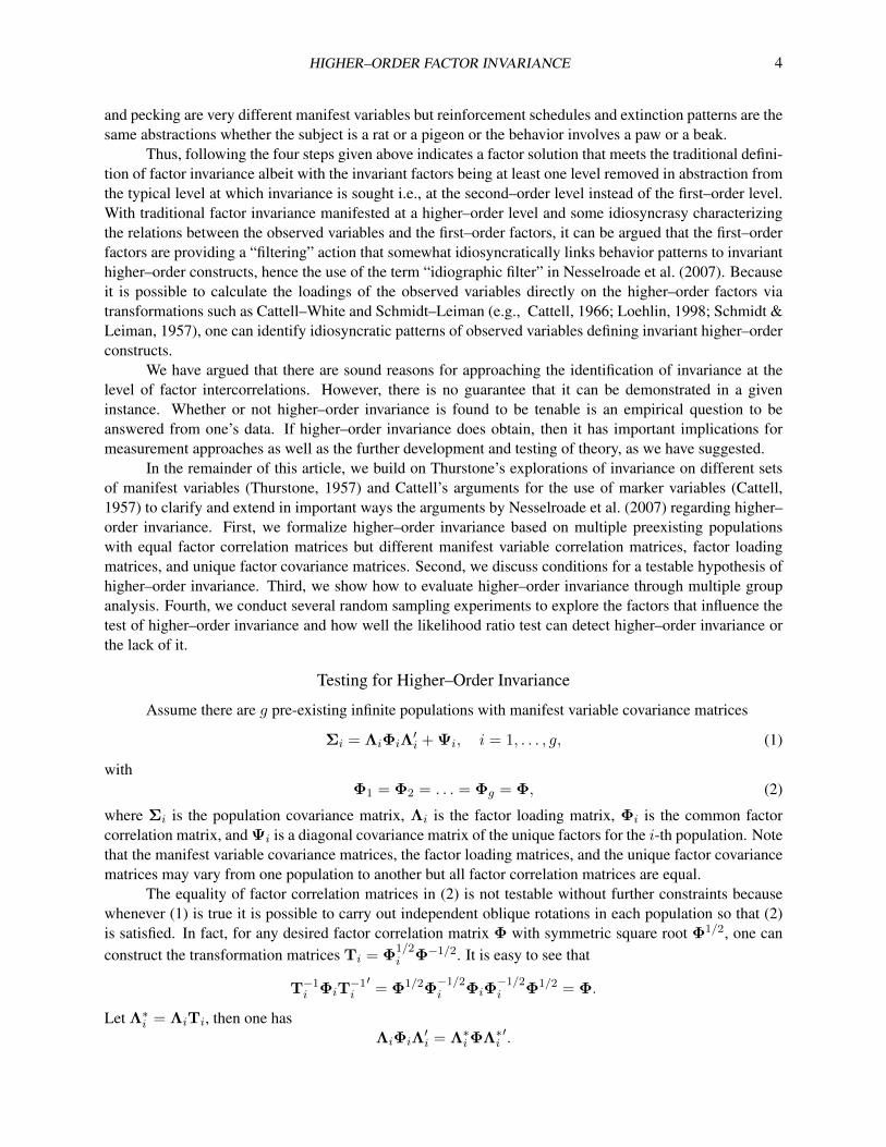
In the remainder of this article, we build on Thurstone’s explorations of invariance on different setsof manifest variables (Thurstone, 1957) and Cattell’s arguments for the use of marker variables (Cattell,1957) to clarify and extend in important ways the arguments by Nesselroade et al. (2007) regarding higher–order invariance. First, we formalize higher–order invariance based on multiple preexisting populationswith equal factor correlation matrices but different manifest variable correlation matrices, factor loadingmatrices, and unique factor covariance matrices. Second, we discuss conditions for a testable hypothesis ofhigher–order invariance. Third, we show how to evaluate higher–order invariance through multiple groupanalysis. Fourth, we conduct several random sampling experiments to explore the factors that influence thetest of higher–order invariance and how well the likelihood ratio test can detect higher–order invariance orthe lack of it.

Testing for Higher–Order Invariance

Assume there are g pre-existing infinite populations with manifest variable covariance matrices

Σi = ΛiΦiΛ′i + Ψi, i = 1, . . . , g, (1)

withΦ1 = Φ2 = . . . = Φg = Φ, (2)

where Σi is the population covariance matrix, Λi is the factor loading matrix, Φi is the common factorcorrelation matrix, and Ψi is a diagonal covariance matrix of the unique factors for the i-th population. Notethat the manifest variable covariance matrices, the factor loading matrices, and the unique factor covariancematrices may vary from one population to another but all factor correlation matrices are equal.

The equality of factor correlation matrices in (2) is not testable without further constraints becausewhenever (1) is true it is possible to carry out independent oblique rotations in each population so that (2)is satisfied. In fact, for any desired factor correlation matrix Φ with symmetric square root Φ1/2, one canconstruct the transformation matrices Ti = Φ

1/2i Φ−1/2. It is easy to see that

T−1i ΦiT−1i′= Φ1/2Φ

−1/2i ΦiΦ

−1/2i Φ1/2 = Φ.

Let Λ∗i = ΛiTi, then one hasΛiΦiΛ

′i = Λ∗iΦΛ∗i

′.


Thus, before (2) can represent a testable hypothesis, it is necessary to identify each Λi under obliquerotation. The rotation could be done through any method such as direct quartimin (Browne, 2001; Jennrich,2007). After rotation, the hypothesis in (2) could then be tested. However, failing to reject the null hypothesisin (2) is not sufficient to conclude that higher–order factor invariance holds.3 For example, it is conceivablethat one might find equality of two factor correlation matrices representing two totally different domains, apoint made by several of the commentators who discussed Nesselroade et al. (2007).

Thus, additional conditions are required to make sure that a factor from one population matchesthe corresponding factor from another population. One way is to match factors by “theory”, “inspection”,“psychological intuition of meaning”, or “insightful judgments of psychological similarity” (Cattell, 1957;Reyburn & Raath, 1950). Based on these criteria, the identification conditions for Λi, i = 1, . . . , g canbe decided and the factors from the g groups can be matched. Even if the g groups have no variables incommon, the test of factor invariance can still proceed. However, this method may easily fail due to thesubjective decisions that are entailed. Thus, some rigorous decision criteria should be used.

Cattell (1957) suggested the use of marker variables in different studies to match factors. Markervariables are variables introduced into a factor analytic experiment to identify, unambiguously, factors onwhich they are known to be highly loaded. He further suggested that at least two marker variables for eachfactor should be used. The marker variable approach can also be used to investigate the invariance of factorswith different indicating variables in our current application. However, one marker variable for each factorin each group is sufficient to identify the factors given a well-defined factor structure.

We will first illustrate the use of marker variables in a two population example and then discuss theiradvantages. Assume there are three factors –f1, f2, and f3 – in each group. Thus, we need three markervariables, M1, M2, and M3 to match the factors. Further assume there are p1 and p2 manifest variables ineach population, respectively. Besides the common marker variables, the other manifest variables may ormay not be the same in the two populations. The factor loading matrices for the two populations are specifiedin Figure 1. “+” in the figure represents a large positive loading to be estimated for the marker variables,“?” represents loadings of indeterminate magnitude for the non-marker variables and “0” indicates factorloadings that are equal to 0. The marker loading is free to vary without constraint but an attempt shouldbe made to choose marker variables with substantial expected loadings. All other free loadings are fornon-marker variables that can assume any value and for which there is no particular expectation as to theirmagnitude.

Group 1 Group 2f1 f2 f3 f1 f2 f3

M1 + 0 0 M1 + 0 0M2 0 + 0 M2 0 + 0M3 0 0 + M3 0 0 +A1 ? ? ? B1 ? ? ?A2 ? ? ? B2 ? ? ?A3 ? ? ? B3 ? ? ?...

......

......

......

...Ap1 − 3 ? ? ? Bp2 − 3 ? ? ?

1

Figure 1: A demonstration of the use of marker variables. + indicates freely-estimated positive markervariable loadings. ? represents all other free loadings which can assume any values, depending on the data.

3Molenaar (2008) in a written commentary on Nesselroade et al. (2007) noted this as a problem needing to be solved if higher–order invariance is to be formalized.


There are several advantages of using marker variables besides its automatic role for model identi-fication. First, they provide researchers a substantive basis on which to match factors so matching factorsacross studies can retain a theory–driven, substantive flavor. Second, given a firm substrate for the matchingprovided by markers, putatively unique features of the populations or groups can be indulged by includingdifferent non-marker variables in the respective choices of manifest variables. For example, test batteriescan be customized for different groups to better “flesh out” what is conceptualized to be the nature of thefactors in the different groups. Third, sometimes, different groups may react differently to what is ostensiblythe same set of variables, rendering the test batteries functionally different. With the assurance of continuityprovided by marker variables, that different reactions have occurred can be detected in the estimated factorloadings, if they are allowed to vary from group to group. Thus, marker variables can play a valuable rolein the context of building measurement systems that afford a way to make comparisons among individualsor groups while also allowing for idiosyncrasy in the overall measurement schemes. This general line ofreasoning regarding marker variables has much in common with Thurstone’s notion of “factor pure” tests.

Procedure for testing higher–order factor invariance

After matching the factors on the basis of the marker variables, we can assess higher–order factorinvariance through testing Φ1 = Φ2 = . . . = Φg. Now we illustrate the procedure for finite samples.Assume that there are g finite samples that come from the corresponding populations. The sample size ofthe ith sample is ni and there are pi manifest variables (including q marker variables) that indicate q factorsin each sample. Let Si, i = 1, . . . , g denote the observed covariance matrices and Σi = ΛiΦiΛ

′i + Ψi, i =

1, . . . , g denote the model indicated covariance matrix. To identify the model, the factor loadings for themarker variables and non-marker variables are specified as in Figure 1. To estimate the parameters, we canminimize the discrepancy function (e.g., Joreskog, 1971),

F (Σ...; S...) =

g∑i=1

nin

(log |Σi|+ tr(Σ−1i Si)− log |Si| − pi) (3)

where n =∑g

i=1 ni and M... represents short hand denotation of g matrices M1, . . . ,Mg. This discrepancyfunction is a nonnegative scalar valued function that is equal to zero if and only if Σi = Si, i = 1, . . . , g.The discrepancy function value is a useful measure of goodness of fit of a model where a model with betterfit should have a minimum discrepancy function value closer to zero.

To test higher–order factor invariance, consider three models, a saturated model, a non-invariantmodel, and an invariant model. The saturated model, denoted by Model S, is

Model S: Σ(s)i , i = 1, . . . , g are any positive definite matrices. (4)

Note that the minimum discrepancy function is zero for the saturated model at Σ(s)i = Si, i = 1, . . . , g.

The non-invariant model, denoted by Model N, is a g-group factor model with different factor correlationmatrices in each group,

Model N: Σ(n)i = ΛiΦiΛ

′i + Ψi, i = 1, . . . , g. (5)

The higher-order invariant model , denoted by Model H, is also a g-group factor model but with the samefactor correlation matrices specified for each group,

Model H: Σ(h)i = ΛiΦΛ′i + Ψi, i = 1, . . . , g. (6)

The invariant model can be constructed from the non-invariant model by setting Φi = Φ for i = 1, . . . , g.Let Σ(0)

... represent the g true population covariance matrices. These are known in a random samplingexperiment but are not known in practice. Let Σ(h)

... denote the g matrices satisfying Model H that minimize


F(Σ(h)... ; S...

)and F

(Σ(h)... ; S...

)is the corresponding minimum discrepancy function value. Furthermore,

let Σ(h)... denote the g matrices satisfying Model H that minimize F

(Σ(h)... ; Σ(0)

...

)and F

(Σ(h)... ; Σ(0)

...

)is the

corresponding minimum discrepancy function value. The statistic nF(Σ(h)... ; S...

)is the likelihood ratio

test statistic for testing Model H as null hypothesis against the saturated model - Model S - as alternative.Its distribution may be approximated by a noncentral chi-square distribution with

g(p− q)2 − (p+ q)

2+ (g − 1)

q(q − 1)

2(7)

degrees of freedom and noncentrality parameter nF(Σ(h)... ; Σ(0)

...

). Similarly, when testing Model N as null

hypothesis against Model S as alternative, the statistic nF(Σ(n)... ; S...

)approximately follows a noncentral

chi-square distribution with

g(p− q)2 − (p+ q)

2(8)

degrees of freedom and noncentrality parameter nF(Σ(n)... ; Σ(0)

...

). Here, Σ(n)

... and Σ(n)... are matrices sat-

isfying Model N and Model S that minimize F(Σ(n)... ; S...

)and F

(Σ(n)... ; Σ(0)

...

)with F

(Σ(n)... ; S...

)and

F(Σ(n)... ; Σ(0)

...

)denoting the corresponding minimum discrepancy function values, respectively.

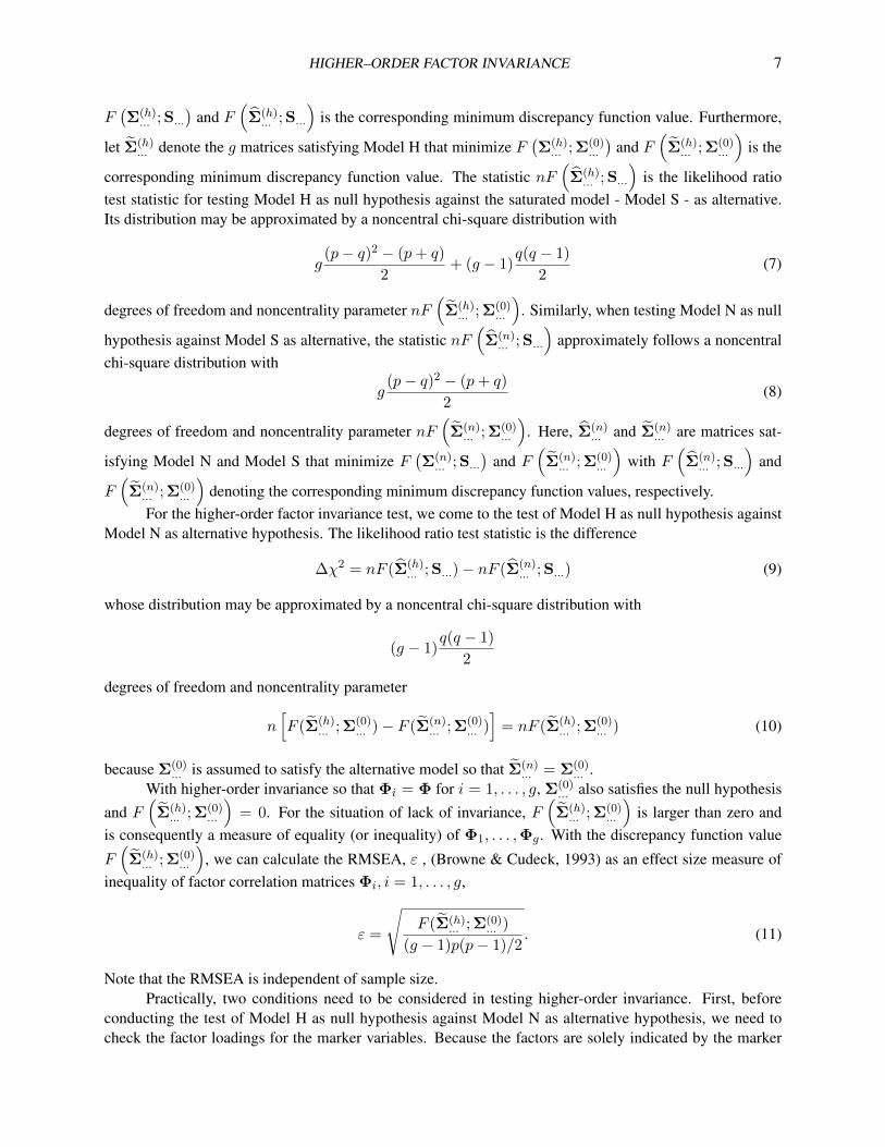
For the higher-order factor invariance test, we come to the test of Model H as null hypothesis againstModel N as alternative hypothesis. The likelihood ratio test statistic is the difference

∆χ2 = nF (Σ(h)... ; S...)− nF (Σ(n)

... ; S...) (9)

whose distribution may be approximated by a noncentral chi-square distribution with

(g − 1)q(q − 1)

2

degrees of freedom and noncentrality parameter

n[F (Σ(h)

... ; Σ(0)... )− F (Σ(n)

... ; Σ(0)... )]

= nF (Σ(h)... ; Σ(0)

... ) (10)

because Σ(0)... is assumed to satisfy the alternative model so that Σ(n)

... = Σ(0)... .

With higher-order invariance so that Φi = Φ for i = 1, . . . , g, Σ(0)... also satisfies the null hypothesis

and F(Σ(h)... ; Σ(0)

...

)= 0. For the situation of lack of invariance, F

(Σ(h)... ; Σ(0)

...

)is larger than zero and

is consequently a measure of equality (or inequality) of Φ1, . . . ,Φg. With the discrepancy function value

F(Σ(h)... ; Σ(0)

...

), we can calculate the RMSEA, ε , (Browne & Cudeck, 1993) as an effect size measure of

inequality of factor correlation matrices Φi, i = 1, . . . , g,

ε =

√F (Σ(h)

... ; Σ(0)... )

(g − 1)p(p− 1)/2. (11)

Note that the RMSEA is independent of sample size.Practically, two conditions need to be considered in testing higher-order invariance. First, before

conducting the test of Model H as null hypothesis against Model N as alternative hypothesis, we need tocheck the factor loadings for the marker variables. Because the factors are solely indicated by the marker


variables, the factor loadings for the marker variables should be sufficiently large. We suggest visuallyverifying that the loadings are substantial, for example, a loading (after standardization) that is larger than0.5 can be considered as substantial based on substantive theory. Unfortunately, if the loadings for markervariables are too small, such as less than 0.1, we may be forced to conclude that there is no factor invariance.Note that although the marker variables are the common variables across groups, we should not constraintheir non-zero loadings to be the same to avoid unnecessary restrictions on factor loadings.

After verifying that the loadings for marker variables are substantial, we can continue to test theinvariance of factor correlation matrices. We first estimate Φi, i = 1, . . . , g from Model N and obtain thechi-square value χ2

df1 = nF(Σ(n)... ; S...

)with df1 representing the degrees of freedom defined by Eq (8).

Then we set Φ1 = Φ2 = . . . = Φg and obtain the χ2df2 = nF

(Σ(h)... ; S...

)with df2 defined by Eq (8).

If the difference ∆χ2 = χ2df2 − χ2

df1 as the likelihood ratio test statistic is smaller than the critical valuefrom the chi-square distribution with degrees of freedom (g− 1)q(q− 1)/2, we have failed to reject the nullhypothesis and thus conclude that higher–order factor invariance prevails. Otherwise, the factor correlationmatrices are non-invariant.

Differences Between Common Factor Invariance and Higher–Order Invariance

An essential difference between pursuing traditional factor invariance and higher–order invarianceis that the former requires that the same set of variables be used across comparison groups. As shown inFigure 2, for common factor invariance, the same manifest variables A1, A2, A3, A4, and A5 are used forboth groups. However, for higher–order invariance, only the maker variables M1 and M2 need be commonvariables. The other variables can be totally different as is the case with A3, A4, and A5 with B3, B4, andB5.

This difference can be made still clearer by further investigating the definition of factor invariance.If a set of variables X can be decomposed into common and unique factors, X is factorable. If the factormatrix remains the same under selection, X is said to be factorially invariant (Meredith, 1993). Thus,traditional factor invariance focuses on testing the invariance of factor loadings of the same set of manifestvariables across groups (e.g., Horn & McArdle, 1992; Meredith, 1964, 1993). If invariance obtains at thatlevel, the observed variables are argued to have the same meaning or to measure the same construct acrossgroups (e.g., Bollen, 1989; French & Finch, 2006). If this form of invariance does not hold, the observedvariables are construed as showing different meanings in the different subgroups, i.e., the observed variablesare essentially different variables for different groups in which case the latent constructs indicated by theobserved variables are construed as different across groups.4

A prime question for higher–order invariance to answer is whether or not the factors indicated bydifferent sets of variables, the selection of which has been fine-tuned to conform to the features of each mea-sured population, are the same factors. To ensure the factors are from the same domain, prior knowledgecan be used and the marker variable approach discussed earlier is one way to use such knowledge. Demon-strating that the factor loadings of the markers are substantial offers some concrete evidence that the factorsare as hypothesized. Additionally testing the invariance of factor correlation matrices supports an inferencethat the factors are invariant. Identifying the patterns by which different manifest variables load the samefactors further enriches substantive understanding of the factor in different individuals or subgroups.

Random Sampling Experiments

We have discussed reasons for investigating higher–order invariance and how to test for it. In thissection, we explore possible influences on the test of higher–order invariance through random sampling

4Although measurement invariance may exist when factor invariance does not hold (Meredith, 1993), without the latter re-searchers generally conclude that the variables do not measure the same construct.


f1

A1 A2 A3 A4 A5

f2 f1

A1 A2 A3 A4 A5

f2

Common Factor Invariance

Group 1 Group 2

f1

M1 M2 A3 A4 A5

f2 f1

M1 M2 B3 B4 B5

f2

Higher-order Factor Invariance

Group 1 Group 2

Figure 2: The comparisons of the usual factor invariance and higher–order factor invariance. In the topfigure, the correlations between f1 and f2 are freely estimated and the factor loadings are often constrainedto be the same for the two groups. In the bottom figure, the correlations are set to be equal but all factorloadings are freely estimated.

experiments. In the first three experiments, we investigate how the number of non-marker variables, theloadings of marker variables, and the communalities affect the factor correlation estimates. In the fourthexperiment, we look at the performance of the likelihood ratio test in detecting higher–order invariance.

Experiment 1: Using only marker variables

We have indicated how marker variables can be used to identify the same factors under higher orderinvariance conditions. Using only one marker variable for each factor provides a way to test higher–orderinvariance and idiographic features of the non-marker variables simultaneously. However, it is not suitableto use only marker variables for higher–order invariance analysis. If the marker variables alone are used, thenumber of observed variables (p) is equal to the number of marker variables (q), which is also the numberof factors. The estimates of the factor correlations are the manifest variable correlations. It can be shownthat the correlations between manifest variables underestimate the factor correlations.

When p = q, the factor loading matrix Λ = Dλ is a diagonal matrix and thus the population manifestvariable covariance matrix

Σ = DλΦDλ + Dψ,

where Φ is factor correlation matrix, and Dψ is unique factor covariance matrix and is also a diagonal matrix.Let Dσ denote the diagonal matrix formed by the diagonal elements of Σ. Then P = D

−1/2σ ΣD

−1/2σ

becomes the manifest variable correlation matrix and

P = DζΦDζ + D∗ψ

where Dζ = D−1/2σ Dλ and D∗ψ = D

−1/2σ DψD

−1/2σ . The population factor correlation matrix Φ are thus

related to P by the attenuation formulae

Off[P] = Off[DζΦDζ ]


where Off[A] represents the matrix formed from the off-diagonal elements of A with zeros in the diagonaland Dζ is also a diagonal matrix of square roots of communalities. Because communalities lie between zeroand one, the correlation between the manifest variables are in general smaller than correlations betweenfactors. Consequently, sample correlations between manifest variables will be both biased and inconsistentestimators of correlations between factors.

For the purpose of demonstration, let p = q = 3 and set

Λ =

.707 0 00 .707 00 0 .707

Φ =

1 .5 .4.5 1 .3.4 .3 1

,then the manifest variable correlation matrix is (the communalities are set at .5)

P =

1 .25 .2.25 1 .15.2 .15 1

.Clearly, in this simple example the correlations of manifest variables are only half the size of the corre-sponding correlations between factors.

Experiment 2: The effect of non-marker variables

We have shown that using only the marker variables is not sufficient to obtain accurate factor corre-lation estimates. Now, we investigate how the number of non-marker variables influences the estimation ofthe factor correlation matrix. Increasing the number of non-marker variables increases the model degrees offreedom which are determined by

df =(p− q)2 − (p+ q)

2.

For the purpose of demonstration, we set q = 3 and change the value of p. We compare the factor correlationestimates with p = 6, 9, 12, and 15, corresponding to factor models with 2, 3, 4 and 5 indicating variablesfor each of the three factors. The factor correlation matrix is set as

Φ =

1 .5 .4.5 1 .3.4 .3 1

, (12)

and the uniqueness covariance matrix Ψ = (ψij)is set as ψii = 0.5, i = 1, . . . , p and ψij = 0, i 6= j, i, j =1, . . . , p. With this setting, all communalities have been chosen to be 0.5 so that effects due to an arbitrarychoice of different communalities are avoided.

The specification of the factor loading matrices for models with the increasing number of non-markervariables (different p) is given in Table 1. The degrees of freedom for the four models are 0, 12, 33, and 63,respectively. Note that when adding non-marker variables we specify the factor loadings to be the same asthe other non-marker variables to control the effects of the magnitude of the factor loadings.

To compare the factor correlation estimates with different numbers of non-marker variables, we sim-ulate R sets of data using the factor loading matrix specifications in Table 1 and estimate the factor corre-lations. Let φ(r)ij denote the estimated factor correlation between the i-th and j-th factors obtained from the

r-th replication and let φ(o)ij be the corresponding population value. Furthermore, let zr stand for the AverageSquared Error (ASE) measure of accuracy of Φ obtained from the r-th replication where

zr =2

q(q − 1)

q∑j=2

j−1∑i=1

(φ(r)ij − φ

(o)ij )2.


Table 1: The influences of non-marker variables on factor correlation estimates

model Λ df EASE CI

p = 6, q = 3

.707 0 00 .707 00 0 .707.410 .410 .000.000 .439 .439.422 .000 .422

0 .01437 [.01429, .01446]

p = 9, q = 3

.707 0 00 .707 00 0 .707.410 .410 .000.000 .439 .439.422 .000 .422.410 .410 .000.000 .439 .439.422 .000 .422

12 .00808 [.00804, .00812]

p = 12, q = 3

.707 0 00 .707 00 0 .707.410 .410 .000.000 .439 .439.422 .000 .422.410 .410 .000.000 .439 .439.422 .000 .422.410 .410 .000.000 .439 .439.422 .000 .422

33 .00722 [.00717, .00727]

p = 15, q = 3 −∗ 63 .00674 [.00670, .00678]Note. df: degrees of freedom. ∗: The factor loading matrix here has the samestructure as the one above with three more observed non-marker variables.The factor loading matrix is omitted to save space.

The Expected Average Squared Error (EASE, denoted by µz) as a measure of accuracy of the esti-mates of Φ for a model can be estimated by

z =1

R

R∑r=1

zr.

Furthermore, a 100(1−α)% confidence interval for EASE could be constructed based on the Central LimitTheorem using

z − nα/2sz√R≤ µz ≤ z + nα/2

sz√R,

where nα/2 is the 100(1− α/2) percentile of the standard normal distribution and

s2z =1

R− 1

R∑r=1

(zr − z)2.

Table 1 presents the EASE and its 95% confidence interval for the factor correlation estimates fromdifferent models with the sample size of 500 based on R = 100, 000 replications. The results clearlyshow that with more non-marker variables, the EASE becomes smaller. The confidence intervals for theEASE do not overlap for the four models. Thus, the use of non-marker variables can help estimate the factorcorrelations more accurately. Furthermore, based on the magnitude of the EASE, it seems that increasing thenumber of non-marker variables makes a big difference initially but an asymptote appears to be approachedwith further increases.


Table 2: The influences of factor loadings and communalities on factor correlation estimates

Model Λ ζ2 EASE CI

M1

.707 0 00 .707 00 0 .707.410 .410 .000.000 .439 .439.422 .000 .422.410 .410 .000.000 .439 .439.422 .000 .422

.5

.5

.5

.5

.5

.5

.5

.5

.5

.00808 [.00804, .00812]

M2

.707 0 00 .707 00 0 .707.707 .000 .000.000 .707 .000.000 .000 .707.707 .000 .000.000 .707 .000.000 .000 .707

.5

.5

.5

.5

.5

.5

.5

.5

.5

.00638 [.00635, .00641]

M3

.316 0 00 .316 00 0 .316.707 .000 .000.000 .707 .000.000 .000 .707.707 .000 .000.000 .707 .000.000 .000 .707

.1

.1

.1

.5

.5

.5

.5

.5

.5

.04771 [.04747, .04794]

M4

.707 0 00 .707 00 0 .707.316 .000 .000.000 .316 .000.000 .000 .316.316 .000 .000.000 .316 .000.000 .000 .316

.5

.5

.5

.1

.1

.1

.1

.1

.1

.02311 [.02299, .02323]

Note. ζ2: Communalities.

Experiment 3: The effects of factor loadings and communalities

To investigate whether the distribution of factor loadings and the magnitude of the communalitiesinfluence the factor correlation estimates, we designed an experiment in the following way. First, the factorcorrelation matrix is the same as in Experiment 2 and the number of manifest variables is fixed at 9. Fourmodels with different factor loading matrices and communalities are summarized in Table 2

To compare the factor correlation estimates, we again obtain the EASE for each model based onR = 100, 000 replications of simulation with the sample size 500. The EASE and its 95% confidenceinterval for the four models are given in Table 2. Models M1 and M2 have the same communalities (0.5) butModel M2 has a simpler structure than Model M1. The EASEs from the two models are very close althoughoverall M2 seems to have better factor correlation estimates. The difference between M2 and M3 lies in thecommunalities for marker variables in M3 being much smaller. The much larger EASE for M3 comparedto M1 indicates that low communalities in marker variables can severely reduce the accuracy of the factorcorrelation estimates. M3 and M4 have the same factor structure. However, M3 has low communalities onthe marker variables while M4 has low communalities on the non-marker variables. The much lower ASEAfor M4 compared to M3 suggests that the communalities of marker variables play a more important rolethan those of non-marker variables in estimating the factor correlations.


Experiment 4: Finite sample properties of likelihood ratio test for higher-order invariance

We have suggested the use of the likelihood ratio test for higher–order invariance. Asymptotically,the likelihood ratio test statistic ∆χ2 has a non-central chi-square distriubtion. However, the performanceof the test in detecting higher-order invariance and lack of invariance in finite samples is yet to be evaluated.Thus, in this simulation experiment, we investigate how well the likelihood ratio test can detect higher–orderinvariance. In other words, we evaluate how well the non-central chi-square distribution can approximatethe empirical distribution of the likelihood ratio test statistics.

Simulation design. The simulation focuses on the higher–order invariance of two populations(groups). For the first group, the population parameters are set as in M1 in Table 2. For the second group, thepopulation parameters are determined according to the effect size of the inequality of the factor correlations.

The RMSEA (ε) in Eq (11) can be used as a measure of effect size in factor correlation inequalityin this experiment. To determine the population RMSEA, we need to know Σ(0)

... and it is known only inrandom sample experiments. For the two group in the experiment, the factor correlation matrices are set,respectively, as

Φ1 =

[1 .5 .4.5 1 .3.4 .3 1

]and Φ2 =

[1 .5 + d .4 + d

.5 + d 1 .3 + d

.4 + d .3 + d 1

], (13)

where d is the difference between corresponding factor correlations of the two groups in the experiment. Tofacilitate comparisons, the communalities are always fixed at 0.5. Thus, the factor loadings are different fordifferent effect sizes. Furthermore, the variances for the unique factors are always fixed at 0.5.

Under these specifications, for each value of d, the population covariance matrices Σ(0)... are deter-

mined and the RMSEA can be calculated. In this experiment, we implemented four levels of RMSEA: 0,0.05, 0.08, and 0.12 corresponding to zero, small, medium, and large effect sizes, respectively. For the fourlevels of RMSEA, the corresponding d values are 0, −.227, −.35, and −.499, respectively.

The likelihood ratio test statistic has an asymptotic non-central chi-square distribution with d =(g − 1)q(q − 1)/2 degrees of freedom and noncentrality parameter δ = d(n1 + n2)ε

2 where n1 and n2 aresample sizes of the two simulated groups, respectively. Note that when the RMSEA is ε = 0, there existshigher-order invariance and the noncentrality parameter is 0.

In this experiment, we obtained the empirical distribution for the likelihood ratio test statistic basedon R = 2000 simulation replications for sample sizes at n1 = n2 = 100 to 500 with an interval of 100 foreach of the two groups. For each simulation replication, the likelihood ratio test statistic was retained as thechi-square difference (∆χ2

i , i = 1, . . . , R) between the invariance model and the non-invariance model.

Simulation results. Let χ21−α(3) be the critical value of a chi-square distribution with d = (g −

1)q(q−1)/2 = 3 degrees of freedom at the level α. With the likelihood ratio test statistic from Monte Carlosimulation, we calculated α by

α =#[∆χ2

i > χ21−α(3)]

R,

where #[∆χ2i > χ2

1−α(3)] is the number of replications of simulation where ∆χ2i exceeded χ2

1−α(3). WhenRMSEA = 0, the α is the estimated Type I error and when the RMSEA >0, the α is estimated power.

For the simulation, the asymptotic non-central chi-square distribution for the likelihood ratio statisticis known. Thus, we can calculate

α = Pr[χ2(3, δ) > χ21−α(3)]

where δ = d(n1+n2)ε2 and χ2(d, δ) denotes a non-central chi-square distribution with d degrees of freedom

and non-centrality parameter δ. Note when RMSEA = 0, δ = 0 and thus α = α. If the non-central chi-square distribution can approximate the distribution of the likelihood test statistics well, we should expectthat α is close to α.


Table 3: Comparison of the empirical distribution and the non-central chi-square approximation distributionof the likelihood ratio test statistic

Sample size (n1 = n2)RMSEA d 100 200 300 400 500

0 0 0.087 0.068 0.065 0.059 0.052α 0.05 -0.227 0.185 0.267 0.411 0.515 0.618

0.08 -0.35 0.370 0.636 0.817 0.917 0.9630.12 -0.499 0.675 0.947 0.990 1.000 1.000

0 0 0.05 0.05 0.05 0.05 0.05α 0.05 -0.227 0.153 0.275 0.400 0.518 0.623

0.08 -0.35 0.345 0.634 0.824 0.924 0.9700.12 -0.499 0.692 0.951 0.995 1.000 1.000

Table 3 presents α and α with different sample sizes and effect sizes when α = 0.05. When RMSEA= d = 0, α is the proportion of simulations that reject the null hypothesis that there is higher-order invari-ance. With small sample sizes, α is greater than the nominal level 0.05. With increased sample size, it comescloser to 0.05. When RMSEA> 0, α and α are measures of power in detecting non-invariance. Overall,with increased sample size, the power increases. Across the rows of the table, α is close to α especially witha greater RMSEA.

To further investigate possible deviations of the non-central chi-square distribution from the empiricaldistribution of the likelihood ratio test statistic, we compared the estimated density of the likelihood ratio teststatistic directly with the non-central chi-square density. The density functions for the likelihood ratio teststatistic from a sample of 2,000 Monte Carlo replications were estimated by applying the filtered polynomialmethod, originally proposed by Elphinstone (1983, 1985) and resuscitated by Heinzmann (2008).5

Figure 3 portrays the histograms and estimated density functions for the likelihood ratio test statisticsin this experiment. First, it clearly shows that the estimated density functions using the filtered polyno-mial method capture the characteristics of the corresponding histograms. Second, it demonstrates that thedistribution of the likelihood ratio test statistics does not seem to change with increased sample size whenRMSEA = 0. Third, it also demonstrates that the distribution of the likelihood ratio test statistic approachessymmetry and the variation of the test statistic increases as the sample size and RMSEA increase, providedthat RMSEA > 0.

To enable a further comparison of the estimated actual distribution of the likelihood ratio test statisticwith the asymptotic non-central chi-square distribution, Q-Q plots are shown in Figure 4. The ordinate ofeach graph represents values of the quantile function of the noncentral chi-square distribution, χ2(d, δ).Degrees of freedom d, are

d = g(g − 1)q(q − 1)/2 = 1 · 3 · 2/2 = 3

throughout. The noncentrality parameter, δ is a function of total sample size, n1 + n2, and of the RMSEA,ε, given by

δ = d(n1 + n2)ε2.

For example, if the RMSEA is ε = 0.05 and n1 = n2 = 200, then the noncentrality parameter is δ = 3. Theabscissa of the graph represents corresponding values of the quantile function of the actual distribution ofthe likelihood ratio test statistic. This function was estimated when applying the filtered polynomial methodto the sample of 2000 Monte Carlo replications. To avoid displaying inaccurate regions of the Q-Q plotoccurring in the tails, it is shown only between the 1st and 99th percentiles of the noncentral chi-squaredistribution.

Figure 4 suggests that this non-central chi-square approximation to the likelihood ratio test statistic isfully adequate over the ranges of values of the RMSEA and sample sizes considered except possibly when

5We thank Dr. Guangjian Zhang for his help with the density plots.


0 20 40 60 80 100

0.00

0.10

0.20

Likelihood ratio statistic

Pro

babi

lity

(a) RMSEA=0 & n1=n2=100

0 20 40 60 80 100

0.00

0.10

0.20


Pro

babi

lity

(b) RMSEA=0 & n1=n2=300

0 20 40 60 80 100

0.00

0.10

0.20


Pro

babi

lity

(c) RMSEA=0 & n1=n2=500

0 20 40 60 80 100

0.00

0.10

0.20


Pro

babi

lity

(d) RMSEA=.05 & n1=n2=100

0 20 40 60 80 100

0.00

0.10

0.20


Pro

babi

lity

(e) RMSEA=.05 & n1=n2=300

0 20 40 60 80 100

0.00

0.10

0.20


Pro

babi

lity

(f) RMSEA=.05 & n1=n2=500

0 20 40 60 80 100

0.00

0.10

0.20


Pro

babi

lity

(g) RMSEA=.12 & n1=n2=100

0 20 40 60 80 100

0.00

0.10

0.20


Pro

babi

lity

(h) RMSEA=.12 & n1=n2=300

0 20 40 60 80 100

0.00

0.10

0.20


Pro

babi

lity

(i) RMSEA=.12 & n1=n2=500

Figure 3: Histograms and estimated density plots for the likelihood ratio test statistics.


n1 = n2 = 100. The increasing length of the quantile-quantile lines in Figure 4 reflects the increasingvariation of the distribution of the likelihood ratio statistic as sample sizes and RMSEA increase, as seenin Figure3. We conclude from this experiment that the likelihood ratio test can detect both invariance andnon-invariance in the higher-order invariance context.

0 20 40 60 80 100

020

4060

8010

0

Estimated quantiles

Nc

chi−

squa

re q

uant

iles

(a) RMSEA=0 & n1=n2=100

0 20 40 60 80 100

020

4060

8010

0Estimated quantiles

Nc

chi−

squa

re q

uant

iles

(b) RMSEA=0 & n1=n2=300

0 20 40 60 80 100

020

4060

8010

0

Estimated quantiles

Nc

chi−

squa

re q

uant

iles

(c) RMSEA=0 & n1=n2=500

0 20 40 60 80 100

020

4060

8010

0

Estimated quantiles

Nc

chi−

squa

re q

uant

iles

(d) RMSEA=.05 & n1=n2=100

0 20 40 60 80 100

020

4060

8010

0

Estimated quantiles

Nc

chi−

squa

re q

uant

iles

(e) RMSEA=.05 & n1=n2=300

0 20 40 60 80 1000

2040

6080

100

Estimated quantilesN

c ch

i−sq

uare

qua

ntile

s

(f) RMSEA=.05 & n1=n2=500

0 20 40 60 80 100

020

4060

8010

0

Estimated quantiles

Nc

chi−

squa

re q

uant

iles

(g) RMSEA=.12 & n1=n2=100

0 20 40 60 80 100

020

4060

8010

0

Estimated quantiles

Nc

chi−

squa

re q

uant

iles

(h) RMSEA=.12 & n1=n2=300

0 20 40 60 80 100

020

4060

8010

0

Estimated quantiles

Nc

chi−

squa

re q

uant

iles

(i) RMSEA=.12 & n1=n2=500

Figure 4: QQ plot. The abscissa and ordinate represent the quantiles from estimation based on the filteredpolynomial density function and the non-central chis-square distribution, respectively. The dotted line is thereference line with slope equal to 1.

Discussion and Conclusions

Measurement remains one of the most vital concerns of the behavioral and social sciences. A lackof valid measurement approaches foregoes any hope of empirically testing theoretical constructions thatmight lead to explanation and thus limits scientific progress to continued descriptive work. Researchers in


behavioral and social science measurement have not been idle and over the past four or five decades wehave benefited from extensions of classical test theory (Lord & Novick, 1968), innovations deriving frommathematical psychology (Krantz & Tversky, 1971), the development of item response theory (IRT) (Rasch,1960), the introduction and subsequent development of generalizability theory (Cronbach, Gleser, Nanda, &Rajaratnam, 1972; Shavelson, Webb, & Rowley, 1989), and so on. For the past three decades a major pointof concentration has been the development and elaboration of the measurement model approach within theframework of structural equation modeling (SEM). This last springs from the common factor analysis modeland relies heavily on the rich traditions of factorial invariance to build a measurement scheme that explicitlyconfronts various reliability, validity, and scaling issues.

Despite the promise and popularity of SEM-based measurement approaches, we have found themwanting when they are evaluated in light of what we believe to be the role of the individual as the unit of anal-ysis in a science of behavior. The essential arguments, which have been presented elsewhere (Nesselroade etal., 2007), and were summarized above, identify a “filtering” role for factors to eliminate idiosyncrasy thatis irrelevant, yet present and detrimental to the purpose of establishing lawful relations. This role for factorswas referred to as “the idiographic filter” by Nesselroade et al. (2007). A proposed solution, and the onefeatured herein, is to invoke the logic and methods of factorial invariance at the level of the interrelationsamong the primary factors while allowing the associated primary factor loadings to reflect idiosyncraticfeatures of individuals or subgroups. This then provides an invariant reference frame for the higher–orderconstructs while allowing them to project into the measurement space in non-invariant patterns. For exam-ple, transformations such as the Schmidt-Leiman and Cattell-White transformations (Loehlin, 1998) can beused to obtain the loadings of observed variables on the higher order factors.

Although the strategy just described seems to be a promising way to nullify unwanted idiosyncrasywhile enhancing measurement properties, one obviously cannot be completely “laissez-faire” in mappingfactor loading patterns to individuals or subgroups. Even though the procedures constrain the primary factorsto intercorrelate identically across individuals or subgroups and thus dictate invariant second order factorpatterns (what we have labeled higher–order invariance), for the procedure to yield a convincing solutionone wants to have confidence that the somewhat different factor loading patterns still represent the “same”underlying factors. This needs to be more substantial than just a “feeling” and, as was discussed earlier,there are minimum loading pattern conditions to be observed in establishing higher–order invariance. At thesame time, however, it was made clear that there is absolutely no requirement that identical variable sets arenecessary for establishing factorial invariance, even in the traditional sense of that term.

That individuals and subgroups differ in important ways in how they construe verbal items, in theirlearning/conditioning histories, etc., seems ample reason for entertaining the possibility that a rigidly stan-dardized measurement framework at the observable level may not be the most appropriate and compellingway to proceed with the assessment of abstract constructs. Admittedly, this assertion “flies in the face” ofmeasurement tradition in behavioral and social science but, rather than being rejected outright, the poten-tial value of such an approach needs to be assessed. The simulation studies we conducted leant supportto the higher–order invariance conception as a viable and promising option for constructing and evaluatingidiosyncratically tailored schemes for measuring abstract constructs. What are some of the more generalimplications of these proposals and the supporting results that we have reported here? Here are three worthnoting.

1. Recognizing and actively nullifying idiosyncrasy that is irrelevant to one’s measurement purpose butwhich can intrude into the process of empirical inquiry, rather than ignoring it, leaving it to “averageout,” is possible and methods and techniques for so doing deserve to be further elaborated and applied,even though they may challenge long-held beliefs regarding “proper” measurement in the social andbehavioral sciences.

2. To the extent that idiosyncrasy in standardized measurement frameworks tends to dilute the strength


of relations among important constructs, getting rid of it through filtering operations such as thosediscussed herein can be expected to result in stronger relations.

3. In the higher–order invariance context, the design of studies can be innovative in building measure-ment batteries that are better matched to one’s experimental aims. For example, longitudinal studiescan deliberately plan to mold the nature of the test battery to the age-level of the participants at eachoccasion of measurement while maintaining their research focus on the same constructs. In cross-sectional studies involving subgroup comparisons based on age, ethnicity, gender, etc., test batteriescan be tailored to the subgroup while still measuring the same constructs.

Finally, along with various colleagues we reiterate the importance of re-focusing on the individualas the proper unit of analysis in psychological research (see e.g., Carlson, 1971; Lamiell, 1997; Molenaar,2004; Nesselroade & Molenaar, 2010). The study of individual differences, despite its popularity andproductivity, still needs to work at “reconstituting” a meaningful individual from all those differences thatare studied. The higher order invariance conception that we have examined herein is aimed at helpingto promote an individual emphasis by offering a more informed basis for aggregating information aboutindividuals in the effort to articulate general relations. Clearly, however, the emphases and the approachextend to comparisons at the subgroup level as well as the individual level.


References

Baltes, P. B., & Nesselroade, J. R. (1970). Multivariate longitudinal and cross–sectional sequences for analyzingontogenetic and generational change: A methodological note. Developmental Psychology, 2, 163–168.

Bollen, K. A. (1989). Structural equations with latent variables. New York : Wiley.Browne, M. W. (2001). An overview of analytic rotation in exploratory factor analysis. Multivariate Behavioral

Research, 36(1), 111–150.Browne, M. W., & Cudeck, R. (1993). Alternative ways of assessing model fit. In K. A. Bollen & J. Long (Eds.),

Testing structural equation models (pp. 136–162). Newbury Park, CA: Sage.Browne, M. W., & Nesselroade, J. R. (2005). Representing psychological processes with dynamic factor models:

Some promising uses and extensions of ARMA time series models. In A. Maydeu–Olivares & J. J. McArdle(Eds.), Psychometrics: A festschrift to Roderick P. McDonald (pp. 415–452). Mahwah, NJ: Lawrence ErlbaumAssociates.

Carlson, R. (1971). Where is the person in personality research? Psychological Bulletin, 75(3), 203–219.Cattell, R. B. (1957). Personality and motivation structure and measurement. New York: World Book Co.Cattell, R. B. (Ed.). (1966). Handbook of multivariate experimental psychology. Chicago: Rand McNally.Cronbach, L. J., Gleser, G. C., Nanda, H., & Rajaratnam, N. (1972). The dependability of behavioral measurement:

Theory of generalizability for scores and profiles. New York: Wiley.Elphinstone, C. D. (1983). A target distribution model for nonparametric density estimation. Communications in

Statistics, A, Theory and Methods, 12(2), 161–198.Elphinstone, C. D. (1985). A method of distribution and density estimation. Unpublished ph. d. thesis, University of

South Africa, Pretoria, South Africa.French, B. F., & Finch, W. H. (2006). Confirmatory factor analytic procedures for the determination of measurement

invariance. Structural Equation Modeling: A Multidisciplinary Journal, 13(3), 378-402.Heinzmann, D. (2008). A filtered polynomial approach to density estimation. Computational Statistics, 23, 343–360.Horn, J. L., & McArdle, J. J. (1992). A practical and theoretical guide to measurement invariance in aging research.

Experimental Aging Research, 18, 117–144.Jennrich, R. I. (2007). Rotation methods, algorithms, and standard errors. In R. Cudeck & R. C. MacCallum (Eds.),

Factor analysis at 100: Historical developments and future directions (pp. 315–336). Mahwah, NJ: LawrenceErlbaum Associates, Inc.

Joreskog, K. G. (1971). Simultaneous factor analysis in several populatons. Psychometrika, 36, 409-426.Krantz, D. H., & Tversky, A. (1971). Conjoint-measurement analysis of composition rules in psychology. Psycholog-

ical Review, 151–169.Lamiell, J. T. (1997). Individuals and the differences between them. In R. Hogan, J. A. Johnson, & S. Briggs (Eds.),

Handbook of personality psychology (pp. 117–141). New York: Academic Press.Loehlin, J. C. (1998). Latent variable models: An introduction to factor, path, and structural analysis (4th ed.).

Mahwah, NJ: Lawrence Erlbaum Associates.Lord, F. M., & Novick, M. R. (1968). Statistical theories of mental test scores. Reading, MA: Addison-Wesley

Publishing Company.McArdle, J. J. (1982). Structural equation modeling of an individual system: Preliminary results from ”A case study

in episodic alcoholism”. (Unpublished manuscript, Department of Psychology, University of Denver)Meredith, W. (1964). Notes on factorial invariance. Psychometrika, 29, 177–185.Meredith, W. (1993). Measurement invariance, factor analysis and factor invariance. Psychometrika, 58, 525–543.Millsap, R. E., & Meredith, W. (2007). Factorial invariance: Historical perspectives and new problems. In R. Cudeck

& R. C. MacCallum (Eds.), Factor analysis at 100: Historical developments and future directions (pp. 131–152). Mahwah, New Jersey: Lawrence Erlbaum Associates.

Molenaar, P. C. M. (1985). A dynamic factor model for the analysis of multivariate time series. Psychometrika, 50,181–202.

Molenaar, P. C. M. (2004). A manifesto on psychology as idiographic science: Bringing the person back into scientificpsychology – this time forever. Measurement: Interdisciplinary Research and Perspectives, 2, 201–218.

Molenaar, P. C. M. (2008, January). Personal communication.Nesselroade, J. R. (1970). Application of multivariate strategies to problems of measuring and structuring long–term

change. In L. R. Goulet & P. B. Baltes (Eds.), Life–span developmental psychology: Research and theory (pp.193–207). New York: Academic Press.


Nesselroade, J. R., & Estabrook, C. R. (2008). Factor invariance, measurement, and studying development over thelifespan. In C. K. Hertzog & H. Bosworth (Eds.), Festschrift for K. W. Schaie. Washington, D. C.: AmericanPsychological Association.

Nesselroade, J. R., Gerstorf, D., Hardy, S. A., & Ram, N. (2007). Idiographic filters for psychological constructs.Measurement: Interdisciplinary Research and P erspectives, 5, 217–235.

Nesselroade, J. R., McArdle, J. J., Aggen, S. H., & Meyers, J. M. (2002). Alternative dynamic factor models formultivariate time–series analyses. In D. M. Moskowitz & S. L. Hershberger (Eds.), Modeling intraindividualvariability with repeated measures data: Advances and techniques (pp. 235–265). Mahwah, NJ: LawrenceErlbaum Associates.

Nesselroade, J. R., & Molenaar, P. C. M. (2010). Emphasizing intraindividual variability in the study of developmentover the lifespan. In W. F. Overton (Ed.), Handbook of lifespan development. New York: John Wiley & Sons.

Rasch, G. (1960). Probabilistic models for some intelligence and attainment tests. Copenhagen: Danmarks Paeda-gogiske Institut.

Reyburn, H., & Raath, M. (1950). Primary factors of personality. British journal of mathematical and statisticalpsychology, 3, 150-158.

Schmidt, J., & Leiman, J. (1957). The development of hierarchical factor solutions. Psychometrika, 22(1), 53–61.Shavelson, R. J., Webb, N. M., & Rowley, G. L. (1989). Generalizability theory. American Psychologist, 44(2),

922–932.Thurstone, L. L. (1947). Multiple factor analysis. Chicago: University of Chicago Press.Thurstone, L. L. (1957). Multiple factor analysis (fifth impression). Chicago: University of Chicago Press.Zevon, M., & Tellegen, A. (1982). The structure of mood change: Idiographic/nomothetic analysis. Journal of

Personality and Social Pyschology, 43, 111–122.

Higher–Order Factor Invariance and Idiographic Mapping of ...

Documents

Transcript of Higher–Order Factor Invariance and Idiographic Mapping of ...